


1. Introduction
Manufacturing processes can rarely reach infinite accuracy; therefore, every design is subject to manufacturing deviations. Usually, manufacturing tolerances are defined, so that parts can be assembled, while making sure functional clearances or fits are respected. However, besides these assembly and functional features, manufacturing deviation can have a significant impact on the ultimate performance and even operational range of a machine (Guenat & Schiffmann Reference Guenat and Schiffmann2019). A machine design, which offers evenly high performance over a large tolerance set is said to be robust. Various methods and definitions of robust design have been explored over the years. Hasenkamp, Arvidsson & Gremyr (Reference Hasenkamp, Arvidsson and Gremyr2009) define robustness as a systematic effort to achieve insensitivity to sources of unwanted variations. Arvidsson & Gremyr (Reference Arvidsson and Gremyr2008) further identify four principles of robust design: awareness of variation, insensitivity to noise factors and its application in all stages of robust design methodology. Park et al. (Reference Park, Lee, Lee and Hwang2006) decompose robust design into three approaches. First, they consider the Tagushi method, deeming it appropriate for design of experiments (DOE), but criticise the difficulty of finding the proper scale factors to adjust the mean of the objective function to the target value, and the lack of a rigorous mathematical model. Second, robust optimisation is scrutinised: two types of robustness are identified by reducing the change of the objective to variation, and ensuring that constraints satisfy the range of tolerances for the design variables. The sensitivity of a nominal metric – its first derivative – to variations is selected as an objective, while the prohibitive cost of computing the second derivative in a gradient descent optimisation is pointed out. An approximation of the objective function by response surface method (RSM) is recommended to address this challenge. Third, axiomatic design is presented where the goal is to minimise the information content in the design, a strategy similar to Tagushi’s. Their definition of a robust design converges to one, which can keep a high performance under deviations of the design variables from its nominal design point. Hence, insensitivity of the performance metrics to the largest deviations possible is the target. Under this definition, a robust design can withstand inaccuracies from manufacturing, while ensuring quality operation.
Probabilistic and statistical approaches have been used to model the variability of the objective and to bypass derivative computations. This allows to save computational resources and to perform the design search in reasonable time. McAllister & Simpson (Reference McAllister and Simpson2003) used a probabilistic formulation of collaborative optimisation to perform multidisciplinary robust design optimisation of an internal combustion engine. To this end, they determined the mean and variance of the response by a first-order Taylor expansion under the assumption of small variations. Doltsinis & Kang (Reference Doltsinis and Kang2004) optimised the designs of truss and antenna structures, in which the expected value and the standard deviation of the objective function were to be minimised. Dow & Wang (Reference Dow and Wang2014) applied principal component analysis (PCA) to characterise manufacturing variability of compressor blades. They constructed a probabilistic model of variability using the empirical mean and covariance of deviations. Kumar et al. (Reference Kumar, Nair, Keane and Shahpar2008) saved computational time through a Bayesian Monte Carlo (BMC) simulation. Computational fluid dynamics (CFD) simulations evaluate the aerodynamic performance of the compressor blade, while a probabilistic model estimates the effect of manufacturing deviations.
Robustness as a sensitivity analysis around the nominal point via direct evaluations of the model function has so far not been considered due to its prohibitive computational cost. However, should faster models be available, one could directly compute the effects of deviations, in addition to obtaining valuable information on the boundaries of the design space. As a matter of fact, it is common knowledge that a global maximum or minimum must either be a local one in the interior of the domain, or lies on the boundary of the domain. Hence, an accurate representation of the feasible design space can lead to the generation of previously unknown optimal designs during the optimisation process.
1.1. Nature of the issue
A mathematical definition of robustness that accounts for the sensitivity of the figure of merit with respect to deviations of the decision variables, as well as for the spread of the feasible domain is required. Covering the entire feasible domain under deviations of the design variables of interest from the nominal point, while performing a multi-objective optimisation (MOO), requires a very large number of evaluations for each design to capture a complex response surface, with hundreds of designs evaluated at each iteration within the optimisation loop. Robustness evaluated alongside the nominal performance metric of interest, effectively doubles the number of objectives in the context of MOO problem. The inclusion of robustness in an MOO can therefore be computationally prohibitive, even for low-order models of engineering systems. Faster, yet accurate models are therefore required to substitute existing ones. Such surrogate models are in need of a methodology to generate their training data, to train them, to compute the robustness metric and to deploy them in a MOO.
1.2. Goals and objectives
The goal of this investigation is a unified framework for the accurate and efficient inclusion of design robustness towards manufacturing deviations in a complex MOO design problem. The objectives are (a) a definition of robustness in the context of multiobjective optimisation for robust design (MOORD), (b) a framework for surrogate modelling with artificial neural networks (ANNs), (c) the integration of robustness as an objective and/or a constraint in MOORD and (d) the validation of the above mentioned for the design of a robust small-scale radial compressor.
1.3. Scope of the article
The MOORD framework yields a Pareto front, where it is the designer’s responsibility to select the best tradeoff among the nondominated Pareto solutions. Confronted to the challenge of computational time and/or the lack of access to derivatives, the idea is to use gradient-free optimisations schemes, such as genetic algorithms (GAs) and evolutionary algorithms (EAs). To model the variability of a metric of interest to deviations, it is opted to develop fast surrogate models. Thus, aiming at evaluating directly the metric of interest with a fine resolution within its feasible space. The robustness is then evaluated as a weighted discrete set, and is no longer limited to surface representations but can be extended to hypervolumes. The definition of robustness within the scope of MOO is introduced as MOORD, followed by a presentation of the framework to develop fast surrogate models with feed-forward artificial neural networks (FWANNs).
The methodology is verified on an experimentally validated meanline compressor model (1D). It is used to evaluate centrifugal compressor designs at various operating conditions to generate the data needed to train a FWANN-based surrogate model. Since functioning designs are a minority class, proper training of the surrogate model is ensured via oversampling and a decomposition of the surrogate model into three FWANNs, a preliminary classifier, an efficiency predictor and a pressure ratio predictor. The ideal FWANNs are found via a nested backpropagation (BP)-GA optimisation scheme to identify the best hyperparameters of the network (e.g., learning rate, number of hidden layers and number of nodes) and adapt the weights to minimise the error between ground-truth and predictions. FWANN being highly parallelisable, the robustness of the isentropic efficiency is evaluated as a sensitivity analysis around the nominal point and integrated as an objective in the ensuing EA-driven MOORD, where a design pressure ratio is implemented as a constraint.
The compressor surrogate model is used to optimise a small-scale single stage radial compressor for driving domestic scale heat pumps, while maximising its isentropic efficiency, its efficiency-weighted mass-flow range and its robustness against manufacturing and speed deviations for a given operating point. Further, the influence of the input parameters of the optimisation is discussed, and the underlying phenomena leading to a robust design identified. The resulting Pareto front is investigated and tradeoffs established.
2. Multiobjective optimisation for robust design
In order to be robust, the performance of a design should be insensitive to deviations of manufacturing or operating conditions over the largest possible domain. Mathematically, this can be captured by calculating the hypervolume
 $ {\mathrm{HV}}_f $
of deviations
$ {\mathrm{HV}}_f $
of deviations
 $ \Delta {g}_i $
from the nominal point
$ \Delta {g}_i $
from the nominal point
 $ {g}_i $
, weighted by the average value of the performance metric
$ {g}_i $
, weighted by the average value of the performance metric
 $ f $
of interest. This weighted volume can be computed as a sensitivity analysis around the nominal point as shown in Figure 1.
$ f $
of interest. This weighted volume can be computed as a sensitivity analysis around the nominal point as shown in Figure 1.
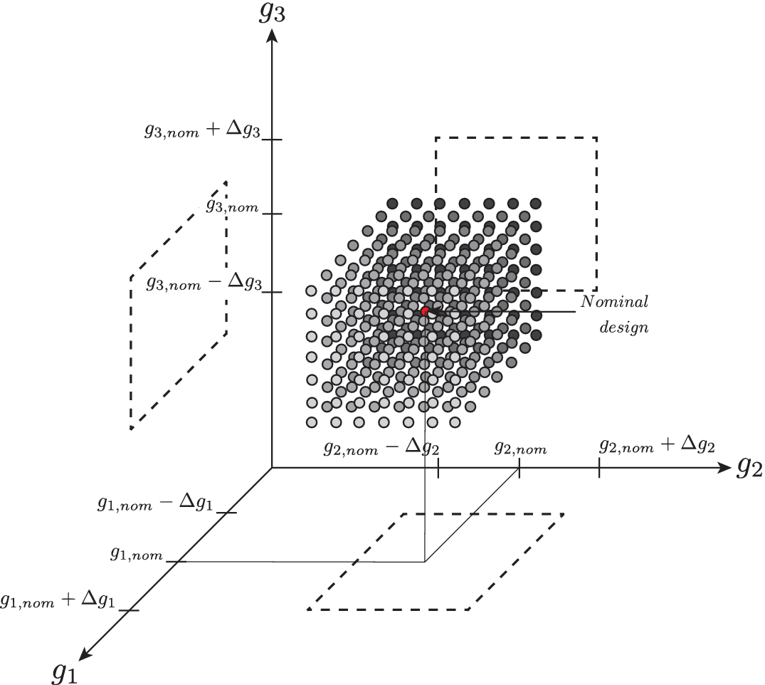
Figure 1. Graphical representation of robustness evaluated as a sensitivity analysis from the nominal point, where the value of the metric of interest is computed at each sampled point. Here, the sensitivity analysis is done with respect to three variables
 $ {g}_1 $
,
$ {g}_1 $
,
 $ {g}_2 $
and
$ {g}_2 $
and
 $ {g}_3 $
. The hypervolume therefore degenerates to a volume, and its projected faces are represented with dashed lines. The red dot in the middle of the hypervolume represents the nominal point, whereas the grey scale of the dot represents the evolution of the considered performance metric.
$ {g}_3 $
. The hypervolume therefore degenerates to a volume, and its projected faces are represented with dashed lines. The red dot in the middle of the hypervolume represents the nominal point, whereas the grey scale of the dot represents the evolution of the considered performance metric.
Definition 1 (Robustness). Given a performance metric
 $ f $
, absolute deviations
$ f $
, absolute deviations
 $ \Delta {g}_i $
of independent variables from the nominal point
$ \Delta {g}_i $
of independent variables from the nominal point
 $ {g}_{i, nom} $
, its robustness is computed with
$ {g}_{i, nom} $
, its robustness is computed with
 $ K $
samples or
$ K $
samples or
 $ {f}_k $
evaluations of the performance metric, as a discrete averaged hypervolume spanning from the nominal point
$ {f}_k $
evaluations of the performance metric, as a discrete averaged hypervolume spanning from the nominal point
 $ {g}_{i, nom} $
 $$ {\mathrm{HV}}_f=\overline{f}\cdot {\Pi}_i\left[\left({g}_{i, nom}+\Delta {g}_i\right)-\left({g}_{i, nom}-\Delta {g}_i\right)\right] $$
with
 $ \overline{f}=\frac{\sum_1^K{f}_k}{K} $
: the performance metric
$ \overline{f}=\frac{\sum_1^K{f}_k}{K} $
: the performance metric
 $ f $
averaged over the swept hypervolume.
$ f $
averaged over the swept hypervolume.
The evaluation of robustness therefore leads to a feasible domain satisfying the constraints and to an unfeasible one that violates constraints as summarised in Figure 2. An optimum design can be found in a local minimum of the feasible domain, or on its boundary. The response surface of design problems is often nonconvex, highly nonlinear and discontinuous. Hence, a large number of additional evaluations are needed around the nominal point to accurately screen both the technically feasible boundaries and the impact on the performance metrics.
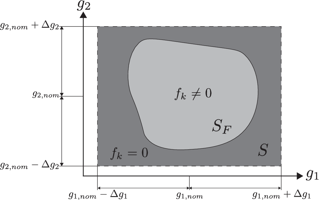
Figure 2. Robustness evaluation of function
 $ f $
leads to a continuous domain defined by
$ f $
leads to a continuous domain defined by
 $ {S}_F $
. Outside of
$ {S}_F $
. Outside of
 $ {S}_F $
, the constraints of the problem are no longer respected and the value of
$ {S}_F $
, the constraints of the problem are no longer respected and the value of
 $ f $
for these samples is set to zero.
$ f $
for these samples is set to zero.
Definition 2 (Feasible domain). The domain
 $ S $
is defined by the absolute deviations of independent variables
$ S $
is defined by the absolute deviations of independent variables
 $ \Delta {g}_i $
from their nominal point
$ \Delta {g}_i $
from their nominal point
 $ {g}_{i, nom} $
(see Figure 2). Under the assumption of continuity, the feasible domain
$ {g}_{i, nom} $
(see Figure 2). Under the assumption of continuity, the feasible domain
 $ {S}_F $
is evaluated within the hypervolume of deviations from the nominal point by applying the
$ {S}_F $
is evaluated within the hypervolume of deviations from the nominal point by applying the
 $ j $
constraints
$ j $
constraints
 $ {h}_1>0,{h}_2>0,\dots {h}_j>0 $
. The evaluations
$ {h}_1>0,{h}_2>0,\dots {h}_j>0 $
. The evaluations
 $ {f}_k $
of the objective function
$ {f}_k $
of the objective function
 $ f $
are set to zero outside the feasible domain
$ f $
are set to zero outside the feasible domain
 $ {S}_F $
.
$ {S}_F $
.
In engineering problems, the design space is often multidimensional, which can make it very challenging to search the entire design space (Goodfellow, Bengio & Courville Reference Goodfellow, Bengio and Courville2016). Moreover, derivatives are not always available to perform gradient descent, or are computationally prohibitive. Heuristic approaches have been developed to explore the space with a lower computational cost, while offering the advantage of searching a maximum or minimum without the need to compute gradients. EA are a class of stochastic optimisation algorithms (Zhou, Yu & Qian Reference Zhou, Yu and Qian2019), which have been successfully applied to solve MOOs of complex engineering systems (Picard & Schiffmann Reference Picard and Schiffmann2020).
Definition 3 (MOO). Given a search space
 $ {S}_{MOO} $
and
$ {S}_{MOO} $
and
 $ p $
objective functions
$ p $
objective functions
 $ {f}_1,{f}_2,\dots, {f}_p $
, the MOO (for maximisation) aims to find the solution
$ {f}_1,{f}_2,\dots, {f}_p $
, the MOO (for maximisation) aims to find the solution
 $ {s}^{\ast } $
satisfying:
$ {s}^{\ast } $
satisfying:
 $$ {s}^{\ast }=\underset{s\in {S}_{MOO}}{\arg \hskip0.1em \mathrm{\max}}f(s)=\underset{s\in {S}_{MOO}}{\arg \hskip0.1em \mathrm{\max}}\left({f}_1(s),{f}_2(s),\dots, {f}_p(s)\right). $$
A MOORD includes the hypervolumes of deviations of each nominal performance metric.
Definition 4 (MOORD). Given a search space
 $ {S}_{MOO} $
and
$ {S}_{MOO} $
and
 $ p $
nominal objective functions
$ p $
nominal objective functions
 $ {f}_{1, nom},{f}_{2, nom},\dots, {f}_{p, nom} $
to be maximised, the robustness of each objective
$ {f}_{1, nom},{f}_{2, nom},\dots, {f}_{p, nom} $
to be maximised, the robustness of each objective
 $ {\mathrm{HV}}_{f_i} $
is included in the MOO as an objective to be maximised. The target solution
$ {\mathrm{HV}}_{f_i} $
is included in the MOO as an objective to be maximised. The target solution
 $ {s}^{\ast } $
then satisfies:
$ {s}^{\ast } $
then satisfies:
 $$ {s}^{\ast }=\underset{s\in {S}_{MOO}}{\arg \hskip0.1em \mathrm{\max}}\left({f}_1(s),{f}_2(s),\dots, {f}_p(s),{HV}_{f_1}(s),{HV}_{f_2}(s),\dots {HV}_{f_p}(s)\right). $$
Hence, extending a nominal MOO to MOORD doubles the number of objectives.
3. Fast modelling with ANNs
ANNs are among the many mathematical tools available in the field of machine learning (ML) to perform classification as well as fast and accurate regression tasks. Working with matrix multiplications, they offer great flexibility in parallelising computation, while offering enough capacity (number of hidden layers and nodes) to approach differential equations (Lagaris, Likas & Fotiadis Reference Lagaris, Likas and Fotiadis1998; Baymani et al. Reference Baymani, Effati, Niazmand and Kerayechian2015). This offers an advantage over Bayesian methods, which require sequential sampling. In this work, the focus is on supervised learning with FWANNs, where the input information is passed from one layer to the next until one or several predicted values are outputted – see Figure 3. Each artificial perceptron or neuron is made of a weighted sum applied to the outputs of the previous layer and an activation function returning the perceptron output. The activation introduces nonlinearity. Among the most common activation functions and their respective first derivatives are the sigmoid function, the hyperbolic tangent or the Rectified Linear Unit (ReLU) (Xu et al. Reference Xu, Wang, Chen and Li2015; Nwankpa et al. Reference Nwankpa, Ijomah, Gachagan and Marshall2018). Several types of cost functions are used to identify the ideal neural network. For classification problems, where a discrete set of output values is to be predicted, categorical cross-entropy (CE) is often used according to Géron (Reference Géron2019). Mean squared error (MSE) or root mean squared error (RMSE) are more often encountered for regression problems, where the goal is to predict a continuous set of outputs.
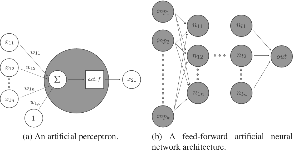
Figure 3. Visualisation of a feed-forward artificial neural network (FWANN) made of several perceptrons and layers. The artificial neuron, or perceptron, takes entries from the previous layers, multiplies them with weights, sums them, inputs the sum into an activation function and returns the result to the perceptrons of the next layer. Perceptrons assembled into hidden layers form the bulk of the FWANN.
A FWANN is trained through BP, where the goal is to minimise the loss function representing the deviations between the predicted and the true values by adjusting the weights and biases of the network, as proposed by Rumelhart, Hinton & Williams (Reference Rumelhart, Hinton and Williams1986). The gradient with respect to the weights can therefore be computed backwards. Thus, the simplest algorithm to find the minimum of the cost function, so as to reduce the error between the predicted and the true values, is gradient descent. By choosing a learning rate
 $ \alpha $
, the weights of the network in each layer are updated iteratively. The same development applies to the biases of the network.
$ \alpha $
, the weights of the network in each layer are updated iteratively. The same development applies to the biases of the network.
Finding the weights of the ANN to minimise the cost function is an optimisation problem, for which BP is an efficient algorithm (Graupe Reference Graupe2013). Gradient descent, however, is prone to getting trapped into local minima of the cost function according to Ruder (Reference Ruder2017). Saddle points can also slow down the training by degenerating the gradient (Goodfellow, Bengio & Courville Reference Goodfellow, Bengio and Courville2016). Solutions, such as introducing noise via mini-batch gradient descent (Montavon, Orr & Müller Reference Montavon, Orr and Müller2012) and optimisers such as Adam (Kingma & Ba Reference Kingma and Ba2017), RMSProp or Nadam (Tato & Nkambou Reference Tato and Nkambou2018) were developed to address these limitations.
Another challenge of surrogate modelling with ANN is the selection of the hyperparameters, such as the number of hidden units, the number of hidden layers, the batch size of training examples to compute the gradient and to perform one iteration of gradient descent, the BP optimiser or the learning rate. Together with the identification of the weights and biases, this leads to a nested optimisation problem, where the ideal ANN hyperparameters for a given problem has to be found first, before performing the BP-driven gradient descent to select the best weights minimising the cost function.
Random search, and EA are among the current state of the art methods applied to select the hyperparameters of an ANN (Papavasileiou, Cornelis & Jansen Reference Papavasileiou, Cornelis and Jansen2021). In this work, an adaptation of the mono-objective GA developed by Harvey (Reference Harvey2017) is used to perform hyperparameter tuning, with the goal of minimising the cost function of the FWANN as represented in Figure 4. The hyperparameters searched by the GA are the following:
-
(i) number of perceptrons per hidden layer,
-
(ii) number of hidden layers,
-
(iii) activation functions,
-
(iv) kernel initialisers for the weights and biases,
-
(v) batch size or number of training examples to compute the gradient and perform one iteration of gradient descent,
-
(vi) optimiser for the BP algorithm and
-
(vii) learning rate to multiply the gradient of the loss function with.
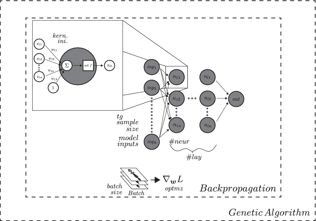
Figure 4. Nested optimisation of a feed-forward artificial neural network. Backpropagation is used in gradient descent to find the best weights and biases minimising the loss function. The hyperparamaters of the network, such as learning rate, number of perceptrons, hidden layers, and so forth are found via genetic algorithm optimisation (hyperparameter tuning).
To avoid overfitting, an L2-regularisation with default parameters is applied. It is a penalty added to the cost function that forces the BP optimisation loop to keep the weight values low.
In this work, the nested optimisation problem for identifying the ideal FWANN, summarised in Figure 4, is implemented as a generic framework. Provided a set of training data and information on the independent variables, it can be used to automatically generate the best possible FWANN in view of obtaining fast and accurate surrogate models that can then be used for MOORD.
4. Case study: compressor performance prediction with neural networks
Designing turbocompressors is an iterative and time-consuming process. It is initialised with a predesign step to identify the tip diameter and rotor speed according to the Cordier line and based on the specified duty (Mounier, Picard & Schiffmann Reference Mounier, Picard and Schiffmann2018). In a second step, a mean line model completed by empirical loss models is used to define the inlet and exhaust areas and blade angles. Then, the channel geometry between the inlet and exhaust is found using a streamline curvature method, which results in a fully define blade geometry. A Reynolds averaged Navier–Stokes (RANS) CFD is then usually performed as a last step to analyse and refine the final geometry of the compressor stage. While an increasing number of design detail is added during each phase, the computational time increases from one design stage to the next. Hence, the initialisation of the design with the first steps is paramount as it hierarchically impacts the following ones.
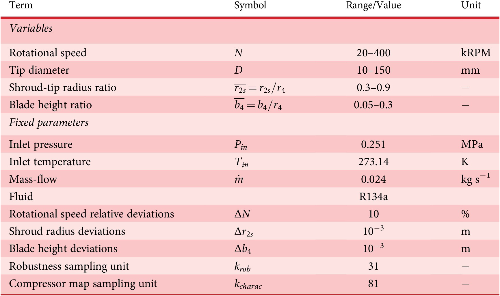
The target application for the case study is a small-scale, one-stage centrifugal compressor for domestic scale heat-pump applications, operating at an inlet pressure
 $ {P}_{\mathrm{in}}=2.51\;\mathrm{bar} $
and temperature
$ {P}_{\mathrm{in}}=2.51\;\mathrm{bar} $
and temperature
 $ {T}_{\mathrm{in}}=273.14\;\mathrm{K} $
, delivering a mass-flow of
$ {T}_{\mathrm{in}}=273.14\;\mathrm{K} $
, delivering a mass-flow of
 $ \dot{m}=0.024 $
kg s−1 and a pressure ratio
$ \dot{m}=0.024 $
kg s−1 and a pressure ratio
 $ \Pi =2 $
, while using halocarbon
$ \Pi =2 $
, while using halocarbon
 $ R134a $
as a working fluid (Schiffmann & Favrat Reference Schiffmann and Favrat2010). The rotational speed
$ R134a $
as a working fluid (Schiffmann & Favrat Reference Schiffmann and Favrat2010). The rotational speed
 $ N $
, the tip diameter
$ N $
, the tip diameter
 $ D $
, the shroud-tip radius ratio
$ D $
, the shroud-tip radius ratio
 $ \overline{r_{2s}} $
and the blade height ratio
$ \overline{r_{2s}} $
and the blade height ratio
 $ \overline{b_4} $
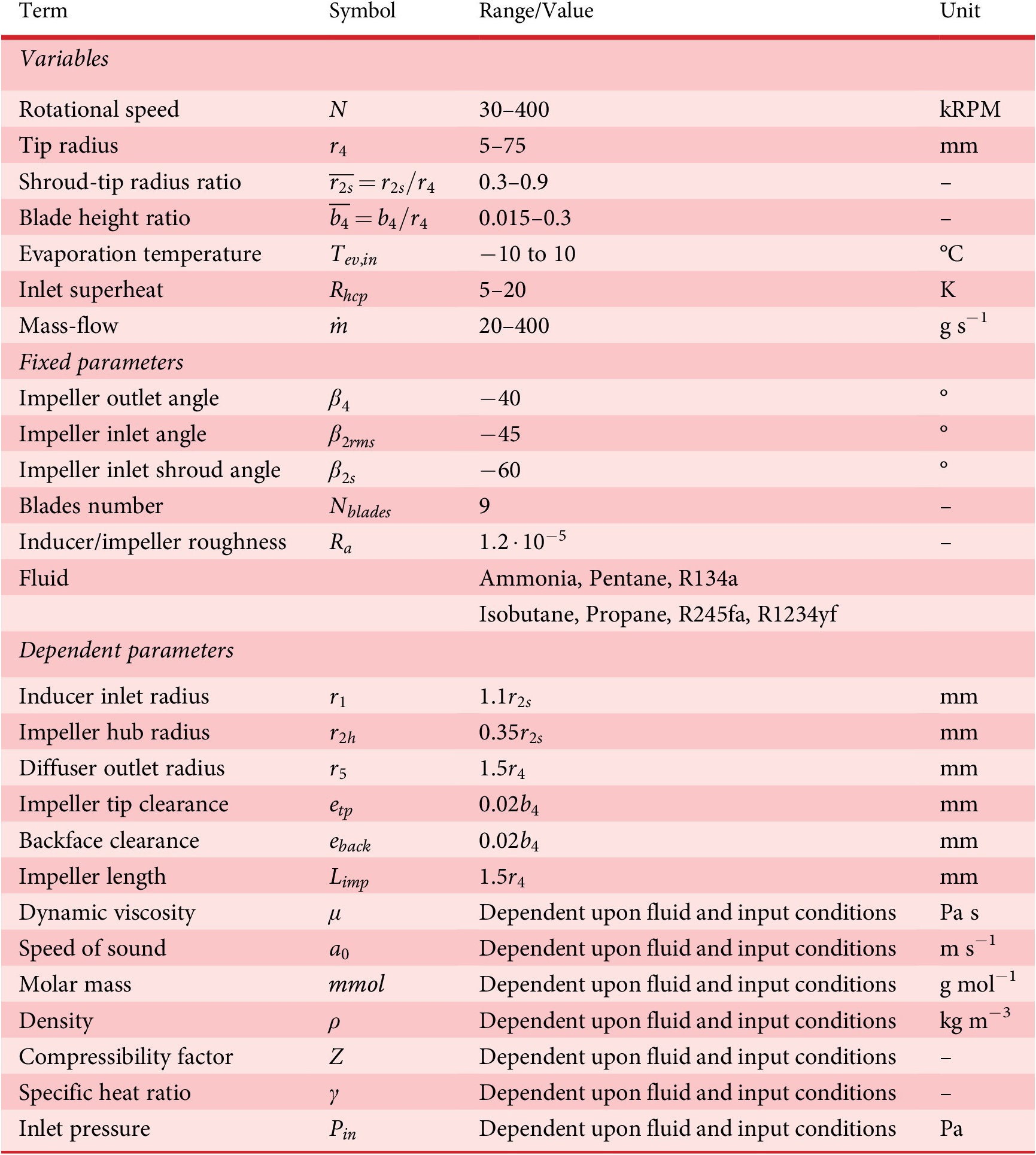
are variables open for optimisation, while all other variables are either dependent or fixed as defined in Table 1.
$ \overline{b_4} $
are variables open for optimisation, while all other variables are either dependent or fixed as defined in Table 1.
Table 1. Description of the inputs of the centrifugal compressor 1D model indicating the ranges considered for the generation of the dataset of the surrogate model
The objective is a robust compressor design, which can withstand geometrical deviations on
 $ {r}_{2s} $
,
$ {r}_{2s} $
,
 $ {b}_4 $
as well as operational deviations on
$ {b}_4 $
as well as operational deviations on
 $ N $
, while maintaining a high isentropic efficiency as well as the design pressure ratio and mass-flow. The manufacturing deviations
$ N $
, while maintaining a high isentropic efficiency as well as the design pressure ratio and mass-flow. The manufacturing deviations
 $ \Delta {r}_{2s} $
and
$ \Delta {r}_{2s} $
and
 $ \Delta {b}_4 $
are imposed on dimensional values to represent the tolerance achieved by a not so accurate lathe, a situation which could be encountered in a mechanical workshop. The relative deviation
$ \Delta {b}_4 $
are imposed on dimensional values to represent the tolerance achieved by a not so accurate lathe, a situation which could be encountered in a mechanical workshop. The relative deviation
 $ \Delta N $
on rotational speed is evaluated alongside manufacturing deviations to investigate the consideration of varying operating conditions within the MOORD. In addition to maximising the efficiency,
$ \Delta N $
on rotational speed is evaluated alongside manufacturing deviations to investigate the consideration of varying operating conditions within the MOORD. In addition to maximising the efficiency,
 $ {\eta}_{\mathrm{is}} $
and robustness
$ {\eta}_{\mathrm{is}} $
and robustness
 $ \mathrm{HV} $
, the efficiency-weighted mass-flow range between surge and choke
$ \mathrm{HV} $
, the efficiency-weighted mass-flow range between surge and choke
 $ \Delta {\dot{m}}_{\Pi =2} $
should also be maximised, in order to offer a wide power modulation range for the heat pump.
$ \Delta {\dot{m}}_{\Pi =2} $
should also be maximised, in order to offer a wide power modulation range for the heat pump.
The identification of the ideal family of compromise between the competing design objectives (efficiency, mass-flow range and robustness) for the specific MOORD problem is addressed by coupling a fast surrogate model to an EA.
4.1. Surrogate model architecture overview
The 1D compressor code developed by Schiffmann & Favrat (Reference Schiffmann and Favrat2010) is based on a meanline model completed with empirical loss models. It can flag numerical errors, surge, choke and functioning states while the outputs are pressure ratio, isentropic efficiency and isentropic enthalpy change for a given geometry and operating conditions. Figure 5 represents the cut view of a centrifugal compressor and its geometric variables needed for the meanline model.
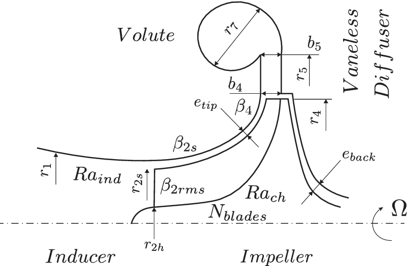
Figure 5. A cut view of the compressor. The shroud-tip radius ratio
 $ \overline{r_{2s}}={r}_{2s}/{r}_4 $
and blade height ratio
$ \overline{r_{2s}}={r}_{2s}/{r}_4 $
and blade height ratio
 $ \overline{b_4}={b}_4/{r}_4 $
, as well as the tip radius
$ \overline{b_4}={b}_4/{r}_4 $
, as well as the tip radius
 $ {r}_4 $
and the rotational speed
$ {r}_4 $
and the rotational speed
 $ \Omega $
are independent variables. All other variables are either dependent of the aforementioned or fixed.
$ \Omega $
are independent variables. All other variables are either dependent of the aforementioned or fixed.
Table 1 summarises all the input variables and their ranges for the meanline compressor model. In order to decrease the number of dimensions, the dimensional variables are made dimensionless by applying the Buckingham-Pi theorem with base variables of
 $ \mathrm{s} $
for time,
$ \mathrm{s} $
for time,
 $ \mathrm{kg} $
for mass,
$ \mathrm{kg} $
for mass,
 $ \mathrm{m} $
for length and
$ \mathrm{m} $
for length and
 $ \mathrm{K} $
for temperature.
$ \mathrm{K} $
for temperature.
 $ \mathrm{mmol} $
is dropped since no other variable with units of
$ \mathrm{mmol} $
is dropped since no other variable with units of
 $ \mathrm{mol} $
is present. This leads to the definition of nondimensional model parameters such as the flow coefficient
$ \mathrm{mol} $
is present. This leads to the definition of nondimensional model parameters such as the flow coefficient
 $ \phi $
, the reduced temperature
$ \phi $
, the reduced temperature
 $ {T}_r $
, the pressure coefficient
$ {T}_r $
, the pressure coefficient
 $ {C}_p $
, the Reynolds number
$ {C}_p $
, the Reynolds number
 $ \mathit{\operatorname{Re}} $
and the Mach number
$ \mathit{\operatorname{Re}} $
and the Mach number
 $ Ma $
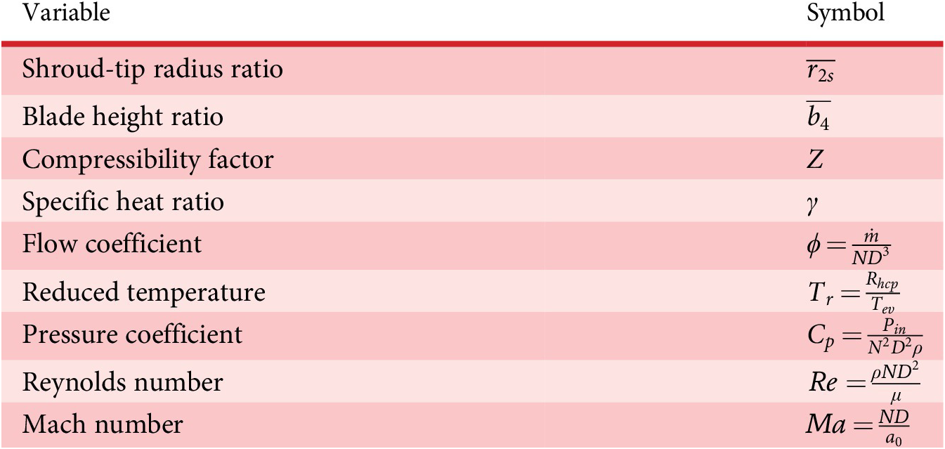
in addition to the shroud-tip and blade height ratios (see Table 2).
$ Ma $
in addition to the shroud-tip and blade height ratios (see Table 2).
Table 2. Set of dimensionless variables used to train the FWANNs to supplant the 1D compressor code
Since discrete predictions of state such as surge and choke, and continuous predictions of efficiency and pressure ratio are targeted, a hierarchical surrogate model has been implemented. In a first step, designs are sent to a classifier ANN that discriminates designs into feasible and nonfeasible (due to choke, surge or numerical modelling error) before stepping into the ANN for the prediction of the isentropic efficiency
 $ {\eta}_{\mathrm{is}} $
and prediction of the pressure ratio
$ {\eta}_{\mathrm{is}} $
and prediction of the pressure ratio
 $ \Pi $
. The workflow of this hierarchical compressor surrogate model is presented in Figure 6.
$ \Pi $
. The workflow of this hierarchical compressor surrogate model is presented in Figure 6.
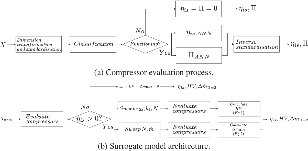
Figure 6. Architecture of the compressor surrogate model. In the compressor evaluation process, design variables
 $ X $
are made dimensionless and standardised. The ANN classifier discriminates functioning designs from the rest and their isentropic efficiency
$ X $
are made dimensionless and standardised. The ANN classifier discriminates functioning designs from the rest and their isentropic efficiency
 $ \eta $
and pressure ratio
$ \eta $
and pressure ratio
 $ \Pi $
is evaluated. These two outputs are inverse standardised. In the surrogate model architecture, this allows for the computation of nominal performance as well as a sweep of values for the computation of robustness
$ \Pi $
is evaluated. These two outputs are inverse standardised. In the surrogate model architecture, this allows for the computation of nominal performance as well as a sweep of values for the computation of robustness
 $ \mathrm{HV} $
and mass-flow modulation
$ \mathrm{HV} $
and mass-flow modulation
 $ \Delta {\dot{m}}_{\Pi =2} $
. Internal constraints are applied to define the feasible regions in each case. The designs and their respective performance are returned.
$ \Delta {\dot{m}}_{\Pi =2} $
. Internal constraints are applied to define the feasible regions in each case. The designs and their respective performance are returned.
In this case study, the design problem is started by defining the variables, the fixed parameters and the dependent parameters of the target compressor design according to Table 1. First, a dataset is randomly sampled using the 1D compressor code. Then, the dimensional parameters are made dimensionless using the Buckingham-Pi theorem. A GA successively trains FWANNs with the transformed data to find the best neural network configuration (hyperparameter identification) for the surrogate model. MSE loss on the test set is used to discriminate one network from the other. Optimum FWANNs are then assembled into a surrogate model mimicking the outputs of the 1D code in a last step.
The MOO of the robust compressor runs with the surrogate model to find the best possible design tradeoffs, that is, maximising efficiency, mas-flow range and robustness. The validity of the FWANNs is further verified by computing the relative error between the 1D code and the FWANNs on each Pareto-optimum compressor design. Finally, design guidelines are drawn from the results and compared with existing results in the literature when applicable.
4.2. Sampling
Based on the work of Mounier, Picard & Schiffmann (Reference Mounier, Picard and Schiffmann2018), a dataset of 4 million points (compressor geometries and operating conditions) is generated through random sampling, for the training of the ANNs. Since 97% of these generated designs are nonfunctioning, the data for the functioning designs is oversampled by sweeping the mass-flow with 4 million extra points. This rises the number of functioning designs to 20% of the dataset. The sampling covers six working fluids to cover representative heat-pump applications. Independent, dependent and fixed parameters as well as their range used for the sampling are summarised in Table 1, while Table 2 shows the subset of nondimensional numbers shown used for the training. Figures A1 and A2 show the distribution of the data as normalised boxplots with respect to the input dimensionless groups of the ANNs.
4.3. Training
A generation of 100 individual FWANNs is generated and evolved over 10 generations for each the classifier, the efficiency and the pressure ratio predictors. The search space of the hyperparameters is defined for the classifier and the predictors in Tables 3 and 4, respectively. The sampled data are split into 60% for training, 20% for validation and 20% for test. Overfitting is avoided using the L2 regularisation on the network weights with a penalty factor of 0.01. An early stopping mechanism is used to save the weights of the network at the epoch with the lowest loss on the validation set. The resulting FWANNs are discriminated with respect to the value of the loss function (CE for the classifier, MSE for the regressions) evaluated on the test set. The best FWANN for a target application across all generations is retained.
Table 3. Description of the hyperparameters searched for the optimisation of the classifier FWANN
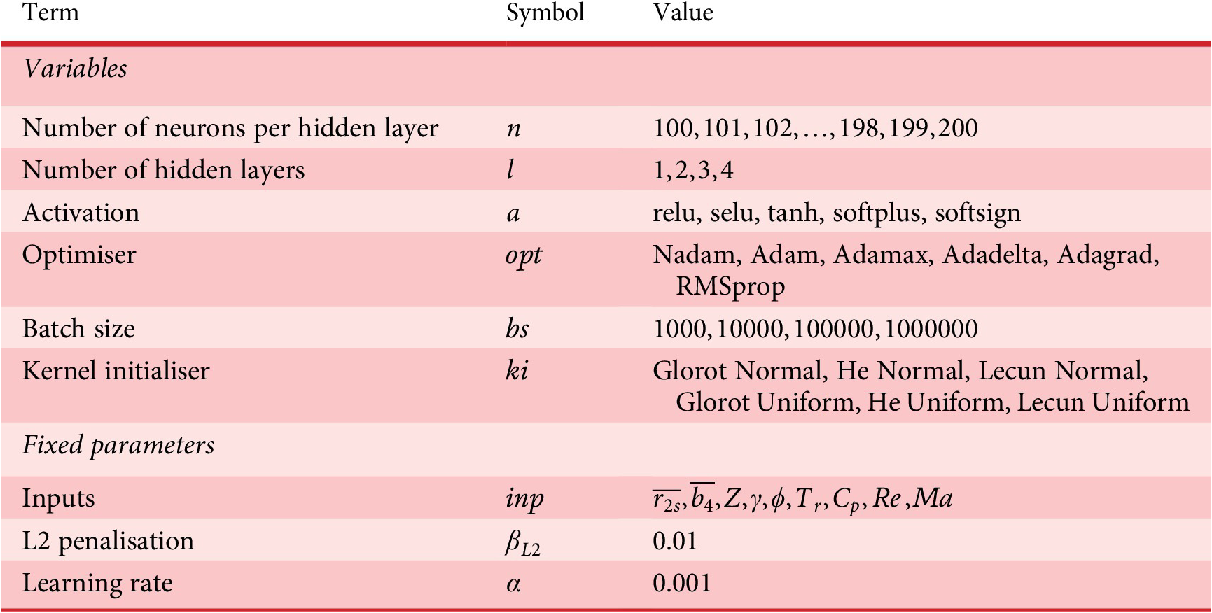
Table 4. Description of the hyperparameters searched for the optimisation of the predictor FWANNs for pressure ratio and isentropic efficiency

4.4. Computation of robustness and evaluation of mass-flow modulation
A matrix of design variables is created at each generation of the EA, where a row represents the nominal design point. For the compressor case study, functioning designs are screened after generating the corresponding dimensionless groups and calling the ANN classifier to discriminate designs into functioning, surge, choke and into numerical error classes.
 $$ {state}_{nom}={ANN}_{classifier}\left(\overline{r_{2s}},\overline{b_4},Z,\gamma, \phi, {T}_r,{C}_p,\mathit{\operatorname{Re}}, Ma\right) $$
The functioning designs are then expanded in a sweep of the shroud radius
 $ {r}_{2s} $
, the blade height
$ {r}_{2s} $
, the blade height
 $ {b}_4 $
, and the speed
$ {b}_4 $
, and the speed
 $ N $
from the nominal point as shown in Figure 1 to assess the effect of dimensional and operational deviation on the design objectives. Each sweep along one dimension is discretised in
$ N $
from the nominal point as shown in Figure 1 to assess the effect of dimensional and operational deviation on the design objectives. Each sweep along one dimension is discretised in
 $ {k}_{rob} $
points for a combinatorial decomposition:
$ {k}_{rob} $
points for a combinatorial decomposition:
 $$ {sweep}_{r_{2s}}= linspace\left({r}_{2s, nom}-\Delta {r}_{2s},{r}_{2s, nom}+\Delta {r}_{2s},{k}_{rob}\right), $$
 $$ {sweep}_{b_4}= linspace\left({b}_{4, nom}-\Delta {b}_4,{b}_{4, nom}+\Delta {b}_4,{k}_{rob}\right), $$
 $$ {sweep}_N= linspace\left({N}_{nom}\cdot \left(1-\Delta N\right),{N}_{nom}\cdot \left(1+\Delta N\right),{k}_{rob}\right). $$
Should the sweeps transgress the lower and upper boundaries of the decision variables as defined per the optimisation, they are changed to match their respective boundaries. The matrix with the swept hypervolume is then evaluated according to the workflow presented in Figure 6, where nonfunctioning designs are associated with zero efficiency and pressure ratio. The objective of robustness of efficiency against manufacturing and operating conditions deviations is then evaluated under the constraints of
 $ 1.9<\Pi <2.1 $
and
$ 1.9<\Pi <2.1 $
and
 $ {\eta}_{\mathrm{is}}>0 $
as follows:
$ {\eta}_{\mathrm{is}}>0 $
as follows:
 $$ \mathrm{HV}=\overline{\eta_{\mathrm{is}}}\cdot \left({r}_{2s,\mathit{\max}}-{r}_{2s,\mathit{\min}}\right)\cdot \left({b}_{4,\mathit{\max}}-{b}_{4,\mathit{\min}}\right)\cdot \left({N}_{max}-{N}_{min}\right) $$
with
 $ \overline{\eta_{\mathrm{is}}} $
: the average efficiency of the sample.
$ \overline{\eta_{\mathrm{is}}} $
: the average efficiency of the sample.
The functioning designs are expanded in a sweep of the mass-flow
 $ \dot{m} $
and the rotational speed
$ \dot{m} $
and the rotational speed
 $ N $
from the nominal point. Each sweep is discretised in
$ N $
from the nominal point. Each sweep is discretised in
 $ {k}_{\mathrm{charac}} $
points as follows:
$ {k}_{\mathrm{charac}} $
points as follows:
 $$ {sweep}_{\dot{m}}= linspace\left({\dot{m}}_{nom}-\Delta \dot{m},{\dot{m}}_{nom}+\Delta \dot{m},{k}_{charac}\right), $$
 $$ {sweep}_N= linspace\left({N}_{nom}\cdot \left(1-\Delta N\right),{N}_{nom}\cdot \left(1+\Delta N\right),{k}_{charac}\right). $$
The matrix of functioning designs is evaluated according to the workflow presented in Figure 6, and surge and choke lines are identified. The objective of mass-flow modulation is then evaluated under the constraints of
 $ 1.9<\Pi <2.1 $
and
$ 1.9<\Pi <2.1 $
and
 $ \eta >0 $
as follows:
$ \eta >0 $
as follows:
 $$ \Delta {\dot{m}}_{\Pi =2}=\overline{\eta_{is}}\cdot \left({\dot{m}}_{choke,\Pi =2}-{\dot{m}}_{surge,\Pi =2}\right) $$
with
 $ \overline{\eta_{is}} $
: the average efficiency of the sample,
$ \overline{\eta_{is}} $
: the average efficiency of the sample,
 $ {\dot{m}}_{surge,\Pi =2} $
: surge mass-flow under constraints and
$ {\dot{m}}_{surge,\Pi =2} $
: surge mass-flow under constraints and
 $ {\dot{m}}_{choke,\Pi =2} $
: choke mass-flow under constraints.
$ {\dot{m}}_{choke,\Pi =2} $
: choke mass-flow under constraints.
4.5. Optimisation methods
The NSGA-III algorithm (Deb & Jain Reference Deb and Jain2014; Jain & Deb Reference Jain and Deb2014) augmented with an adaptive operator selection procedure similar to Vrugt & Robinson (Reference Vrugt and Robinson2007) and Hadka & Reed (Reference Hadka and Reed2013) drives the optimisation of this case study. The Python implementation by pymoo (Blank & Deb Reference Blank and Deb2020) is used. A total of 325 uniformly distributed points following Das & Dennis (Reference Das and Dennis1998) are set as reference directions for NSGA-III. The objectives and constraints are defined below and the parameters and their respective range provided in Table 5:
 $$ {\displaystyle \begin{array}{l}\hskip2em \mathrm{\max}\hskip2em \left({\eta}_{\mathrm{is}},\mathrm{HV},{\Delta}_{{\dot{m}}_{\Pi =2}}\right)\\ {}N,\;D,\;\overline{\;{r}_{2s}},\;\overline{b_4}\\ {}\hskip2em \mathrm{s}.\mathrm{t}.\hskip2em {\eta}_{\mathrm{is}}>0,\\ {}\hskip6.1em 1.9<\Pi <2.1\end{array}} $$
with
Table 5. Description of the parameters for the surrogate compressor model MOORD
 $ {\eta}_{\mathrm{is}} $
: nominal isentropic efficiency,
$ {\eta}_{\mathrm{is}} $
: nominal isentropic efficiency,
HV: hypervolume generated by deviations and weighted by efficiency,
 $ \Delta {\dot{m}}_{\Pi =2} $
: efficiency-weighted achieved mass-flow range at target pressure ratio and
$ \Delta {\dot{m}}_{\Pi =2} $
: efficiency-weighted achieved mass-flow range at target pressure ratio and
 $ \Pi $
: pressure ratio.
$ \Pi $
: pressure ratio.
The procedure for the optimisation of the compressor stage is represented in Figure 7, where the 1D code is replaced by the surrogate model.
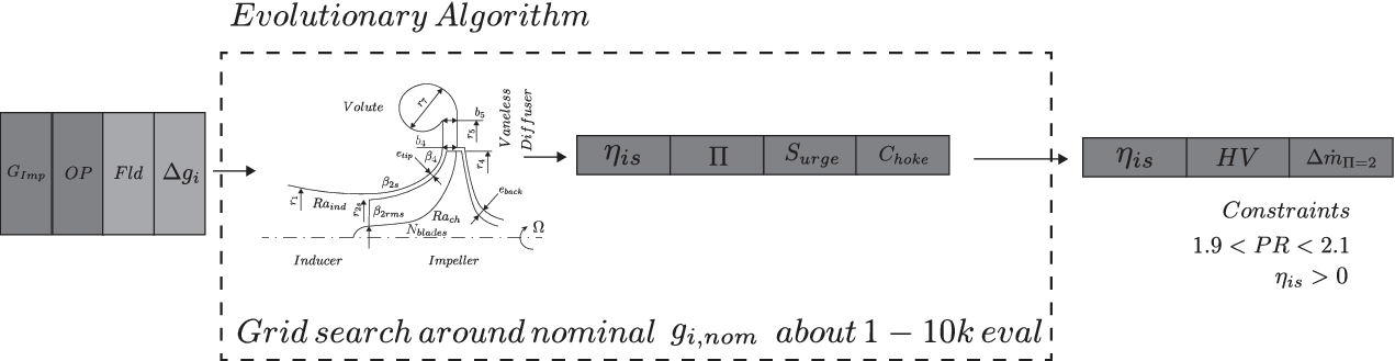
Figure 7. Visualisation of the compressor optimisation. The surrogate model is used to compute the nominal isentropic efficiency
 $ {\eta}_{\mathrm{is}} $
, robustness
$ {\eta}_{\mathrm{is}} $
, robustness
 $ \mathrm{HV} $
and mass-flow modulation
$ \mathrm{HV} $
and mass-flow modulation
 $ \Delta {\dot{m}}_{\Pi =2} $
. It is called only once per generation of the evolutionary algorithm, as a matrix of candidate designs
$ \Delta {\dot{m}}_{\Pi =2} $
. It is called only once per generation of the evolutionary algorithm, as a matrix of candidate designs
 $ {G}_{imp} $
– alongside operating conditions OP, fluid Fld and deviations
$ {G}_{imp} $
– alongside operating conditions OP, fluid Fld and deviations
 $ \Delta {g}_i $
– is inputted and expanded within the model.
$ \Delta {g}_i $
– is inputted and expanded within the model.
5. Results
5.1. ANN training
On the one hand, the use of GA to select the best ANNs alleviates the tedious task of manually searching the network hyperparameters. On the other hand, it comes with a computational cost. As a matter of fact, it took about 4 days to design the ANN classifier, and 1 day for each of the predictor ANNs (pressure ratio and efficiency) on a Nvidia RTX 2080 Ti. The benefit of this procedure, however, is that it leads to the identification of an optimal ANN for a given design problem. In particular, since the tool is made generic enough to automatically create the best ANN to map an input to an output for complex engineering problems. Table 6 summarises the hyperparameters of the three ANNs for the surrogate compressor model.
Table 6. Hyperparameters of the ANNs
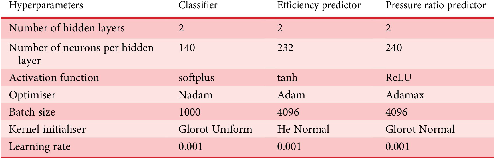
The best identified multiclass classifier has two hidden layers, 140 neurons per hidden layer, uses a softplus activation function, a Glorot Uniform weight initialisation, a batch size of 1000, the Nadam optimiser for the BP with a learning rate of 0.001 and L2 regularisation to avoid overfitting. The training set consists of 4.9 million designs, while the test and validation sets were respectively made of 1.6 million. The classifier ANN has an accuracy and recall of 99% on the functioning class. The average misclassification across the four classes is of 1.83% for a 1.6 million designs test set. The confusion matrix is provided in Figure A3.
The efficiency predictor is trained on a dataset comprising only the functioning designs (2 million designs). The dataset is split in 60/20/20% for training, validation, and testing sets, respectively. The best neural network has two hidden layers, 232 neurons per hidden layer, with the hyperbolic tangent as an activation function, Adam as an optimiser with a learning rate of 0.001, a batch size of 4096, and a He Normal weight initialisation. The achieved MSE on the test set is of 1.18e-3. Figure A4 shows the evolution of the RMSE as a function of epochs for the selected efficiency predictor network.
The pressure ratio predictor is trained on the same dataset as the efficiency predictor. The best neural network found has two hidden layers, 240 neurons per hidden layer, is using the ReLU as an activation function, Adamax as an optimiser with a learning rate of 0.001, a batch size of 4096, and a Glorot Normal weight initialisation. The achieved MSE on the test set is of 5.57e-5. Figure A5 shows the evolution of the RMSE as a function of epochs for the selected pressure ratio predictor network.
Figure 8 shows a computing time comparison between (a) the 1D code running on CPU, (b) the surrogate model made of ANNs running on CPU and (c) the same ANNs running on a GPU. The log–log graph shows a linear trend for the time taken by the 1D code to evaluate compressor designs. There is also a linear increase of the computation time when the ANNs evaluate the designs on CPU. It is, however, about two orders of magnitude faster than the 1D code. The ANNs running on GPU witness a slight increase of computation time with increasing number of evaluations. The computational time difference between the 1D compressor model and the ANN-based surrogate models increases with the number of evaluations. For a single evaluation, the ANNs running on GPU are approximately 40 times faster, while the speed-up factor increases to more than four orders of magnitudes for 120,000 evaluations. This clearly highlights the benefit of running ANNs on GPU. In an EA-driven MOORD generation, about 8 million points are evaluated per generation, which takes in average
 $ 5\pm 1\;\mathrm{s} $
with the FWANN structure on a Nvidia RTX 2080 Ti (GPU). Thus, the data generation investment to train the ANNs is amortised in one generation. In contrast, the 1D-model is sequential and one evaluation takes on average
$ 5\pm 1\;\mathrm{s} $
with the FWANN structure on a Nvidia RTX 2080 Ti (GPU). Thus, the data generation investment to train the ANNs is amortised in one generation. In contrast, the 1D-model is sequential and one evaluation takes on average
 $ 0.19\;\mathrm{s} $
on a single CPU core. Executed on a 8-core Intel i9-9980HK (CPU), the surrogate model based on ANNs still surpasses the 1D code by performing 8 million evaluations in
$ 0.19\;\mathrm{s} $
on a single CPU core. Executed on a 8-core Intel i9-9980HK (CPU), the surrogate model based on ANNs still surpasses the 1D code by performing 8 million evaluations in
 $ 400\pm 21\;\mathrm{s} $
, compared to 20,500 points computed in 586 s for the 1D-model on the same 8-core CPU.
$ 400\pm 21\;\mathrm{s} $
, compared to 20,500 points computed in 586 s for the 1D-model on the same 8-core CPU.
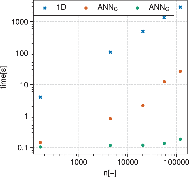
Figure 8. Log–log graph of computation time versus number of design evaluations for the 1D code executed on CPU, the ANNs executed on CPU (subscript C) and the ANNs executed on GPU (subscript G). The computation time is averaged over 10 runs for the ANNs, while single evaluations are summed for the 1D code.
5.2. EA-driven MOORD
The optimisation for efficiency, mass-flow range and hypervolume is run for imposed manufacturing deviations on
 $ {r}_{2s} $
and
$ {r}_{2s} $
and
 $ {b}_4 $
of
$ {b}_4 $
of
 $ 1\times {10}^{-3} $
m, and relative OP deviations of 10% on
$ 1\times {10}^{-3} $
m, and relative OP deviations of 10% on
 $ N $
by coupling the ANN surrogate compressor model to an NSGA-III based EA (Deb & Jain Reference Deb and Jain2014; Jain & Deb Reference Jain and Deb2014).
$ N $
by coupling the ANN surrogate compressor model to an NSGA-III based EA (Deb & Jain Reference Deb and Jain2014; Jain & Deb Reference Jain and Deb2014).
Figure 9 shows the obtained Pareto front and the selected robust design (square marker). The x-axis represents the discrete hypervolume
 $ \mathrm{HV} $
for variations of
$ \mathrm{HV} $
for variations of
 $ {r}_{2s} $
,
$ {r}_{2s} $
,
 $ {b}_4 $
and
$ {b}_4 $
and
 $ N $
under constraints and weighted by efficiency, that is, the robustness of efficiency. The y-axis shows the achieved mass-flow range in the neighbourhood of a pressure ratio of 2. The z-axis, represented by the colormap, displays the nominal isentropic efficiency of the design. The results clearly suggests that the three objectives are competing against each other, that is, maximising one of the objectives will lead to a compromise on the two others.
$ N $
under constraints and weighted by efficiency, that is, the robustness of efficiency. The y-axis shows the achieved mass-flow range in the neighbourhood of a pressure ratio of 2. The z-axis, represented by the colormap, displays the nominal isentropic efficiency of the design. The results clearly suggests that the three objectives are competing against each other, that is, maximising one of the objectives will lead to a compromise on the two others.
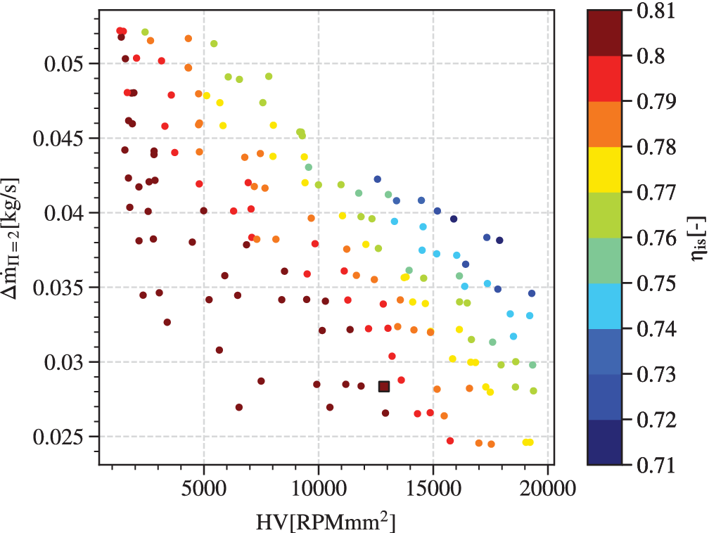
Figure 9. Pareto front for
 $ 1\times {10}^{-3} $
deviation on
$ 1\times {10}^{-3} $
deviation on
 $ {r}_{2s} $
and
$ {r}_{2s} $
and
 $ {b}_4 $
. Robustness
$ {b}_4 $
. Robustness
 $ \mathrm{HV} $
is represented on the x-axis, efficiency-weighted mass-flow modulation
$ \mathrm{HV} $
is represented on the x-axis, efficiency-weighted mass-flow modulation
 $ \Delta {\dot{m}}_{\Pi =2} $
on the y-axis, and the isentropic efficiency
$ \Delta {\dot{m}}_{\Pi =2} $
on the y-axis, and the isentropic efficiency
 $ {\eta}_{\mathrm{is}} $
is represented by a colour gradient. A clear competition between the three objectives is suggested. Aiming at a robust design with high efficiency, the candidate is selected on the Pareto front and represented by a square.
$ {\eta}_{\mathrm{is}} $
is represented by a colour gradient. A clear competition between the three objectives is suggested. Aiming at a robust design with high efficiency, the candidate is selected on the Pareto front and represented by a square.
The relative error between both the isentropic efficiency and the pressure ratio prediction of the ANN and that of the 1D code for the solutions on the identified Pareto front is presented in Figure 10. The colormap suggests that the largest deviation corresponds to an underestimation of −1.2% for mid-range efficiencies, while the highest ones are well predicted. The pressure ratio is predicted even better with the largest relative error ranging between −0.4 and 0.4%.

Figure 10. Relative error, on isentropic efficiency and pressure ratio respectively, for the Pareto optima between the ANN and the 1D code. Pressure ratio is predicted with a better accuracy than isentropic efficiency. The largest relative error observed for efficiency is of −1.2 and 0.4%. The ANN are accurate and conservative with respect to the 1D code.
5.3. Selected solution
The compressor map of the selected solution (square marker in Figure 9) is represented in Figure 11 and its design point as well as nominal performance are summarised in Table 7. The selected design has a well centred compressor map around the nominal operating point, thus yielding a high isentropic efficiency. For an isentropic efficiency higher than 0.74, mass-flow deviations of
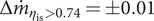 $ \Delta {\dot{m}}_{\eta_{\mathrm{is}}>0.74}=\pm 0.01 $
kg s−1 can be achieved. The (nonweighted) mass-flow range from surge to choke is
$ \Delta {\dot{m}}_{\eta_{\mathrm{is}}>0.74}=\pm 0.01 $
kg s−1 can be achieved. The (nonweighted) mass-flow range from surge to choke is
 $ \Delta \dot{m}=0.038 $
kg s−1. While offering one of the highest efficiencies, the selected solution offers a robustness towards manufacturing and operational deviation higher than the median. Its efficiency-weighted mass-flow range of
$ \Delta \dot{m}=0.038 $
kg s−1. While offering one of the highest efficiencies, the selected solution offers a robustness towards manufacturing and operational deviation higher than the median. Its efficiency-weighted mass-flow range of
 $ \Delta \dot{m}=0.028 $
kg s−1, while being low, is not the lowest of the observed solutions.
$ \Delta \dot{m}=0.028 $
kg s−1, while being low, is not the lowest of the observed solutions.

Figure 11. Compressor map of the selected compressor design. Typical of a high efficiency design, the compressor characteristic is centred on the operating point of
 $ \dot{m}=0.024 $
kg s−1 and
$ \dot{m}=0.024 $
kg s−1 and
 $ \Pi =2 $
. The space on the left is delimited by the surge line, while the one on the right is marked by the choke line. On the edges of the compressor map, the efficiency can drop below 0.71.
$ \Pi =2 $
. The space on the left is delimited by the surge line, while the one on the right is marked by the choke line. On the edges of the compressor map, the efficiency can drop below 0.71.
Table 7. Design point and objectives of the selected design
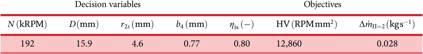
Figure 12 shows the robustness hypervolume for the selected solution. The obliques and convex surfaces of the hypervolume suggest that it has been truncated by the application of the constraints on isentropic efficiency and pressure ratio. The slice of
 $ \mathrm{HV} $
for the nominal speed
$ \mathrm{HV} $
for the nominal speed
 $ {N}_{nom} $
is also presented. For nominal values of
$ {N}_{nom} $
is also presented. For nominal values of
 $ {r}_{2s, nom}=4.6 $
mm and
$ {r}_{2s, nom}=4.6 $
mm and
 $ {b}_4=0.77 $
mm, the design is at a maximum nominal isentropic efficiency of
$ {b}_4=0.77 $
mm, the design is at a maximum nominal isentropic efficiency of
 $ {\eta}_{\mathrm{is}}=0.8 $
. While maintaining the isentropic efficiency above 0.72, deviations of
$ {\eta}_{\mathrm{is}}=0.8 $
. While maintaining the isentropic efficiency above 0.72, deviations of
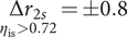 $ \underset{\eta_{\mathrm{is}}>0.72}{\Delta {r}_{2s}}=\pm 0.8 $
mm and
$ \underset{\eta_{\mathrm{is}}>0.72}{\Delta {r}_{2s}}=\pm 0.8 $
mm and
 $ \underset{\eta_{\mathrm{is}}>0.72}{\Delta {b}_4}=\pm 0.2 $
mm can be achieved, which considering the small dimensional values of the nominal design is remarkable.
$ \underset{\eta_{\mathrm{is}}>0.72}{\Delta {b}_4}=\pm 0.2 $
mm can be achieved, which considering the small dimensional values of the nominal design is remarkable.
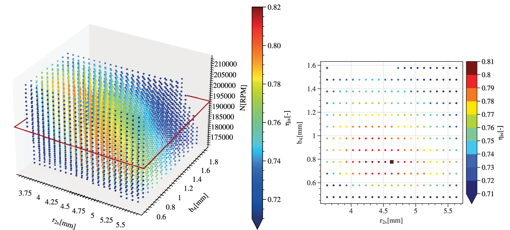
Figure 12. The evaluation of robustness for the selected solution as a hypervolume of deviations from the nominal point is limited to a volume in this case study. Isentropic efficiency at the sampled points is represented by a colour gradient. A slice at the nominal rotational speed is represented on the right. On the edges of the feasible domain, the value of efficiency can drop below 0.71.
5.4. Relationship between variables and objectives
Figure 13 presents the Pareto optima with respect to the variables
 $ Ns $
,
$ Ns $
,
 $ Ds $
,
$ Ds $
,
 $ \overline{r_{2s}} $
and
$ \overline{r_{2s}} $
and
 $ \overline{b_4} $
. The evolution of objectives with respect to the decision variables assembled in pair-plots is represented with a colour gradient spanning from the lowest to the highest observed objective value. The left column of graphs shows the evolution of
$ \overline{b_4} $
. The evolution of objectives with respect to the decision variables assembled in pair-plots is represented with a colour gradient spanning from the lowest to the highest observed objective value. The left column of graphs shows the evolution of
 $ \mathrm{HV} $
, while the middle one addresses variations of
$ \mathrm{HV} $
, while the middle one addresses variations of
 $ \Delta {\dot{m}}_{\Pi =2} $
, and the right one displays variation of
$ \Delta {\dot{m}}_{\Pi =2} $
, and the right one displays variation of
 $ {\eta}_{\mathrm{is}} $
.
$ {\eta}_{\mathrm{is}} $
.
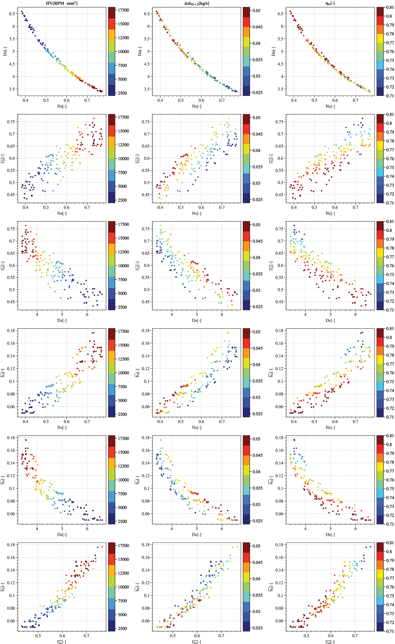
Figure 13. Evolution of each of the four decision variables against the three objectives. Decision variables of the Pareto optima are graphed in pair-plots and coloured by objective value. The left column represents the robustness
 $ \mathrm{HV} $
, while the middle one represents the efficiency-weighted mass-flow range
$ \mathrm{HV} $
, while the middle one represents the efficiency-weighted mass-flow range
 $ \Delta {\dot{m}}_{\Pi =2} $
and the right one the isentropic efficiency
$ \Delta {\dot{m}}_{\Pi =2} $
and the right one the isentropic efficiency
 $ {\eta}_{\mathrm{is}} $
. Specific speed
$ {\eta}_{\mathrm{is}} $
. Specific speed
 $ Ns $
and specific diameter
$ Ns $
and specific diameter
 $ Ds $
instead of
$ Ds $
instead of
 $ N $
and
$ N $
and
 $ D $
are picked to favour comparison.
$ D $
are picked to favour comparison.
Specific speed
 $ Ns $
and specific diameter
$ Ns $
and specific diameter
 $ Ds $
are dimensionless groups used to characterise turbomachinery. The specific diameter (Eq. (13)) and speed (Eq. (14)) correspond to a nondimensional representation of the compressor rotor speed and the compressor tip diameter (Korpela Reference Korpela2020). Larger
$ Ds $
are dimensionless groups used to characterise turbomachinery. The specific diameter (Eq. (13)) and speed (Eq. (14)) correspond to a nondimensional representation of the compressor rotor speed and the compressor tip diameter (Korpela Reference Korpela2020). Larger
 $ Ns $
are typical of axial compressors with larger flow rates, whereas centrifugal machines yield lower
$ Ns $
are typical of axial compressors with larger flow rates, whereas centrifugal machines yield lower
 $ Ns $
due to lower flow rate and higher pressure rise. Specific speeds and diameters of known turbomachines functioning at their best efficiency have been used by Cordier to build the ‘Cordier’ diagram, which identifies the specific diameter for a given specific speed that yields maximum efficiency. It is an early design selection tool created in the 1950s (Dubbel Reference Dubbel2018) that was further extended by Balje in the 1980s (Balje Reference Balje1981).
$ Ns $
due to lower flow rate and higher pressure rise. Specific speeds and diameters of known turbomachines functioning at their best efficiency have been used by Cordier to build the ‘Cordier’ diagram, which identifies the specific diameter for a given specific speed that yields maximum efficiency. It is an early design selection tool created in the 1950s (Dubbel Reference Dubbel2018) that was further extended by Balje in the 1980s (Balje Reference Balje1981).
The first row is a plot of
 $ Ds $
against
$ Ds $
against
 $ Ns $
defined as follows:
$ Ns $
defined as follows:
 $$ Ds=\frac{D{\left|\Delta {h}_{\mathrm{is}}\right|}^{0.25}}{{\left({\dot{m}}_{\mathrm{in}}/\rho \right)}^{0.5}}, $$
 $$ Ns=\frac{\Omega {\left({\dot{m}}_{\mathrm{in}}/\rho \right)}^{0.5}}{{\left|\Delta {h}_{\mathrm{is}}\right|}^{0.75}}, $$
with
 $ \Omega $
: rotational speed in rad/s,
$ \Omega $
: rotational speed in rad/s,
 $ \Delta {h}_{\mathrm{is}} $
: isentropic variation of enthalpy between inlet and outlet,
$ \Delta {h}_{\mathrm{is}} $
: isentropic variation of enthalpy between inlet and outlet,
 $ {\dot{m}}_{\mathrm{in}} $
: inlet mass-flow and
$ {\dot{m}}_{\mathrm{in}} $
: inlet mass-flow and
 $ \rho $
: inlet fluid density in kg m−3.
$ \rho $
: inlet fluid density in kg m−3.
Similar to Mounier, Picard & Schiffmann (Reference Mounier, Picard and Schiffmann2018), the solutions lie within a narrow band of
 $ \left( Ns, Ds\right) $
pairs. There is a clear trend of maximising
$ \left( Ns, Ds\right) $
pairs. There is a clear trend of maximising
 $ \mathrm{HV} $
for higher specific speed and low specific diameter. Increasing
$ \mathrm{HV} $
for higher specific speed and low specific diameter. Increasing
 $ Ds $
and reducing
$ Ds $
and reducing
 $ Ns $
leads to a lower robustness. The inverse trend is observed for the achieved efficiency-weighted mass-flow range between surge and choke,
$ Ns $
leads to a lower robustness. The inverse trend is observed for the achieved efficiency-weighted mass-flow range between surge and choke,
 $ \Delta {\dot{m}}_{\Pi =2} $
, which reduces with higher
$ \Delta {\dot{m}}_{\Pi =2} $
, which reduces with higher
 $ Ns $
and lower
$ Ns $
and lower
 $ Ds $
. The observed correlation is not as strong as for robustness, since there is a limited number of designs with
$ Ds $
. The observed correlation is not as strong as for robustness, since there is a limited number of designs with
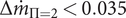 $ \Delta {\dot{m}}_{\Pi =2}<0.035 $
kg s−1 for
$ \Delta {\dot{m}}_{\Pi =2}<0.035 $
kg s−1 for
 $ 0.4< Ns<0.5 $
and
$ 0.4< Ns<0.5 $
and
 $ 5< Ds<6 $
. The trend is weaker for
$ 5< Ds<6 $
. The trend is weaker for
 $ {\eta}_{\mathrm{is}} $
, where designs of low efficiencies can be found for different
$ {\eta}_{\mathrm{is}} $
, where designs of low efficiencies can be found for different
 $ \left( Ns, Ds\right) $
pairs, which corroborates with results by Mounier, Picard & Schiffmann (Reference Mounier, Picard and Schiffmann2018). Note, however, that designs with
$ \left( Ns, Ds\right) $
pairs, which corroborates with results by Mounier, Picard & Schiffmann (Reference Mounier, Picard and Schiffmann2018). Note, however, that designs with
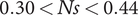 $ 0.30< Ns<0.44 $
and
$ 0.30< Ns<0.44 $
and
 $ 5.6< Ds<6.7 $
all have a very high isentropic efficiency with
$ 5.6< Ds<6.7 $
all have a very high isentropic efficiency with
 $ {\eta}_{\mathrm{is}}>0.79 $
, except one.
$ {\eta}_{\mathrm{is}}>0.79 $
, except one.
The plots in the second row suggest that robustness
 $ \mathrm{HV} $
increases with
$ \mathrm{HV} $
increases with
 $ \overline{r_{2s}} $
and with
$ \overline{r_{2s}} $
and with
 $ Ns $
. For fixed values of
$ Ns $
. For fixed values of
 $ \overline{r_{2s}} $
, increasing
$ \overline{r_{2s}} $
, increasing
 $ Ns $
decreases the mass-flow range
$ Ns $
decreases the mass-flow range
 $ \Delta {\dot{m}}_{\Pi =2} $
. Fixing
$ \Delta {\dot{m}}_{\Pi =2} $
. Fixing
 $ Ns $
while increasing
$ Ns $
while increasing
 $ \overline{r_{2s}} $
leads to a decrease of efficiency
$ \overline{r_{2s}} $
leads to a decrease of efficiency
 $ {\eta}_{\mathrm{is}} $
.
$ {\eta}_{\mathrm{is}} $
.
The third row displays the variation of
 $ \overline{r_{2s}} $
with
$ \overline{r_{2s}} $
with
 $ Ds $
. The
$ Ds $
. The
 $ \mathrm{HV} $
decreases with decreasing
$ \mathrm{HV} $
decreases with decreasing
 $ {r}_{2s} $
and increasing
$ {r}_{2s} $
and increasing
 $ Ds $
.
$ Ds $
.
 $ \Delta {\dot{m}}_{\Pi =2} $
increases for fixed values of
$ \Delta {\dot{m}}_{\Pi =2} $
increases for fixed values of
 $ \overline{r_{2s}} $
and increasing
$ \overline{r_{2s}} $
and increasing
 $ Ds $
.
$ Ds $
.
 $ {\eta}_{\mathrm{is}} $
decreases for fixed values of
$ {\eta}_{\mathrm{is}} $
decreases for fixed values of
 $ Ds $
and increasing
$ Ds $
and increasing
 $ \overline{r_{2s}} $
.
$ \overline{r_{2s}} $
.
The fourth row is a representation of blade height ratio
 $ \overline{b_4} $
against specific speed
$ \overline{b_4} $
against specific speed
 $ Ns $
. Increasing
$ Ns $
. Increasing
 $ \overline{b_4} $
and
$ \overline{b_4} $
and
 $ Ns $
leads to higher values of robustness, while fixing the values of blade height ratio and increasing the specific speed decreases the mass-flow range achieved between surge and choke at a pressure ratio of 2. The opposite trend is observed for isentropic efficiency: fixing
$ Ns $
leads to higher values of robustness, while fixing the values of blade height ratio and increasing the specific speed decreases the mass-flow range achieved between surge and choke at a pressure ratio of 2. The opposite trend is observed for isentropic efficiency: fixing
 $ \overline{b_4} $
and increasing
$ \overline{b_4} $
and increasing
 $ Ns $
leads to higher
$ Ns $
leads to higher
 $ {\eta}_{\mathrm{is}} $
.
$ {\eta}_{\mathrm{is}} $
.
The fifth row represents the variation of
 $ \overline{b_4} $
with respect to
$ \overline{b_4} $
with respect to
 $ Ds $
. Higher robustness
$ Ds $
. Higher robustness
 $ \mathrm{HV} $
is achieved for lower
$ \mathrm{HV} $
is achieved for lower
 $ Ds $
and higher
$ Ds $
and higher
 $ \overline{b_4} $
. The inverse relation decreases
$ \overline{b_4} $
. The inverse relation decreases
 $ \mathrm{HV} $
. Fixing values of
$ \mathrm{HV} $
. Fixing values of
 $ \overline{b_4} $
and increasing
$ \overline{b_4} $
and increasing
 $ Ds $
leads to higher
$ Ds $
leads to higher
 $ \Delta {\dot{m}}_{\Pi =2} $
. Finally, fixing values of
$ \Delta {\dot{m}}_{\Pi =2} $
. Finally, fixing values of
 $ Ds $
and increasing
$ Ds $
and increasing
 $ \overline{b_4} $
leads to reduced efficiency.
$ \overline{b_4} $
leads to reduced efficiency.
The last row displays the evolution of
 $ \overline{b_4} $
with respect to
$ \overline{b_4} $
with respect to
 $ \overline{r_{2s}} $
.
$ \overline{r_{2s}} $
.
 $ \mathrm{HV} $
increases with the shroud-tip radius and blade height ratio. The variation of mass-flow range is less pronounced. The best designs with respect to
$ \mathrm{HV} $
increases with the shroud-tip radius and blade height ratio. The variation of mass-flow range is less pronounced. The best designs with respect to
 $ \Delta {\dot{m}}_{\Pi =2} $
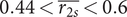
are mainly located in the lower left region, for
$ \Delta {\dot{m}}_{\Pi =2} $
are mainly located in the lower left region, for
 $ 0.44<\overline{r_{2s}}<0.6 $
and
$ 0.44<\overline{r_{2s}}<0.6 $
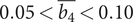
and
 $ 0.05<\overline{b_4}<0.10 $
. Furthermore, the upper region of the band formed by the Pareto optima contains the worst designs with respect to mass-flow modulation.
$ 0.05<\overline{b_4}<0.10 $
. Furthermore, the upper region of the band formed by the Pareto optima contains the worst designs with respect to mass-flow modulation.
6. Discussion
6.1. Artificial neural networks
For the compressor design problem addressed as a case study in this work, a speed-up of four orders of magnitude has been achieved compared to the 1D code using ANN-based surrogate models. This speed-up can be further increased since it is only limited by the memory capacity of the GPU. The relative difference between the 1D code and the ANN-based surrogate model is minimal for the computation of the compressor performance (1.2% maximum difference on the isentropic efficiency and 0.4% on the pressure ratio), while surge and choke are also well predicted. Accurate results coupled with a massive speed-up of the ANNs open the path to a new, faster design process.
Typically, the state-of-the-art turbocompressor design methodology is initialised with a first design that is based on unified performance maps, such as the ones offered by Balje. This starting point provides an idea on the ideal rotor speeds and tip diameter. In the next step, a 1D-meanline methodology model is used to identify the compressor inlet and discharge geometries. High-fidelity models are used only towards the end of the process, and since they are computationally expensive, they are rather used in an analysis mode rather than for design. As a consequence, the bulk of the geometry definition occurs early in the design process. The process of a sequential engagement of more complex models in a design process calls for accurate starting points to minimise the number of design iterations. This is the reason why predesign maps have to be updated, when applications go beyond the validity range of available resources as pointed out by Mounier, Picard & Schiffmann (Reference Mounier, Picard and Schiffmann2018), and by Capata & Sciubba (Reference Capata and Sciubba2012).
However, the replacement of the 1D-meanline model with a much faster ANN-based surrogate model allows to merge the utilisation of the predesign maps and the optimisation with the meanline model into a single and much faster step. In addition, the ANN-based surrogate model can be used to extend the design process to include the performance across the complete compressor map, while including computationally expensive features such as robustness.
The introduced methodology to automatically generate a fast surrogate model therefore opens the door to an efficient robust design process and to a direct evaluation of the entire compressor map, which significantly alleviates the design of compressors that need to satisfy various operating conditions while maximising efficiency and mass-flow range.
6.2. Tradeoffs
The Pareto front in Figure 9 suggest a competition between the three objectives. The robustness to manufacturing deviations cannot be improved while ensuring a high degree of mass-flow range at a fixed pressure ratio. Maximising the nominal isentropic efficiency does not result in a more robust design either. This goes against the common belief that maximising one of the nominal performance metrics will result in increased safety margin when deviating from the nominal point. This corroborates with results by Capata & Sciubba (Reference Capata and Sciubba2012) who found similar results when designing low Reynolds number turbocompressors.
6.3. Design guidelines
Lower rotational speeds, diameters and values of shroud-tip radius ratio and blade height ratio yield a compressor map centred on the highest isentropic efficiency
 $ {\eta}_{\mathrm{is}} $
point for the given operating conditions.
$ {\eta}_{\mathrm{is}} $
point for the given operating conditions.
A design maximising the efficiency-weighted hypervolume
 $ \mathrm{HV} $
compensates a small tip diameter with higher rotational speed, shroud-tip radius and blade height ratios. This is a design with a high specific speed (
$ \mathrm{HV} $
compensates a small tip diameter with higher rotational speed, shroud-tip radius and blade height ratios. This is a design with a high specific speed (
 $ Ns $
) and a low specific diameter (
$ Ns $
) and a low specific diameter (
 $ Ds $
), and high shroud-tip radius ratio (
$ Ds $
), and high shroud-tip radius ratio (
 $ \overline{r_{2s}} $
) and high blade height ratio (
$ \overline{r_{2s}} $
) and high blade height ratio (
 $ \overline{b_4} $
). This leads to a centring of the design in the hypervolume of deviations. These results are in line with Mounier, Picard & Schiffmann (Reference Mounier, Picard and Schiffmann2018) and their description of the evolution of the design space with
$ \overline{b_4} $
). This leads to a centring of the design in the hypervolume of deviations. These results are in line with Mounier, Picard & Schiffmann (Reference Mounier, Picard and Schiffmann2018) and their description of the evolution of the design space with
 $ Ns $
and
$ Ns $
and
 $ Ds $
, while maintaining a good efficiency.
$ Ds $
, while maintaining a good efficiency.
A solution maximising the achieved efficiency-weighted mass-flow range at a pressure ratio of 2
 $ \Delta {\dot{m}}_{\Pi =2} $
is an anti-symmetric design of the one maximising the hypervolume. On the one hand, large
$ \Delta {\dot{m}}_{\Pi =2} $
is an anti-symmetric design of the one maximising the hypervolume. On the one hand, large
 $ Ds $
, small
$ Ds $
, small
 $ Ns $
, and smaller
$ Ns $
, and smaller
 $ {r}_{2s} $
and
$ {r}_{2s} $
and
 $ {b}_4 $
produce a design on the edge of surge. On the other hand, this design allows for a large increase of mass-flow as it is somewhat oversized for its nominal operating conditions.
$ {b}_4 $
produce a design on the edge of surge. On the other hand, this design allows for a large increase of mass-flow as it is somewhat oversized for its nominal operating conditions.
7. Conclusion
In this article, a unified and automated framework to perform robust design in a MOO setting has been presented. Using fast and parallelisable surrogate models such as ANNs, the computation of robustness expressed as a weighted sensitivity analysis from the nominal point can be included both as an objective and/or as a constraint for complex design problems, where the response surface of competing design objectives is highly nonlinear and nonconvex. The generation of data for the surrogate model training and testing and the relevant oversampling to alleviate unbalanced classes has been described, as well as the nested BP-GA optimisation to train the neural networks and find the best hyperparameters and weights to minimise the prediction error.
This framework was then applied to the design of a small-scale radial compressor. Nominal isentropic efficiency, mass-flow modulation and robustness of isentropic efficiency were included as objectives in an NSGA-III driven MOO under constraints of pressure ratio in the vicinity of two, and feasible design (no surge and no choke). The optimisation results clearly suggest a tradeoff between isentropic efficiency, mass-flow range and robustness, which discards a common practice that maximising one of the performance metrics necessarily offers a higher degree of robustness towards operational and manufacturing deviation. Further, the use of FWANNs suggests an acceleration of the computational time by four orders of magnitude compared to the original 1D meanline base code thanks to parallel computing on GPU, for a deviation below 1.2% on the prediction of the performance metrics (isentropic efficiency and pressure ratio). Within the frame of compressor design, the novel design methodology allows unprecedented possibilities in early design phases, such as the introduction of robustness towards manufacturing and operational deviation as well as the assessment of the compressor across the complete compressor map. Compared to state of the art approaches that require design maps and time-consuming modelling, this is made possible by benefiting from the significant decrease of the computational cost by using ANNs as a means to replace high-fidelity models.
Future work should focus on analysing prediction outliers from the neural networks and assess the risk they pose for the quality of the converged Pareto front. A retraining process of the surrogate model based on Pareto solutions should also be implemented to reduce prediction error on solutions of interest. More design variables should also be included to allow for a wider variety of compressor designs.
Finally, this work can be summarised by the following achievements:
-
(i) Definition of robustness in the context of MOO as a weighted hypervolume defined by the geometrical/operational deviations around a nominal design point, weighted by the average performance metrics of interest. The high number of additional points to compute the hypervolume calls for high speed models. The surrogate model framework developed in this work offers sufficient speed-up to compute robustness in the context of a MOORD.
-
(ii) Development of a generic framework to create FWANN-based surrogates of high-fidelity models for diverse engineering applications. The framework is designed so that the identification of the ideal ANN hyperparameters is formulated as an optimisation problem. As a consequence the neural network topology is automatically adapted to the complexity of the underlying model.
-
(iii) Parallelisable FWANNs reduce the computational time by four orders of magnitude compared to the original compressor 1D code. The speed-up is a combination of the surrogate model architecture and of the fact that the neural networks can be evaluated by hyperparallelisation on GPU. As a consequence, in order to be able to fully capitalise on the ANNs for design, it is highly recommended to use a GPU instead of a CPU.
-
(iv) A robust design of a radial compressor was optimised four orders of magnitude faster than with a meanline 1D code with direct evaluations of deviations and the construction of a compressor map within the optimisation loop. This method is disruptive and can help the engineer to select the optimal tradeoffs for a given compressor application, and move forward with the design process including robustness and the evaluation of the full compressor map in a timely fashion.
Nomenclature
Roman Symbols
-
 $ a $
$ a $
-
speed of sound/ANN activation function (m s −1 )
-
$ b $
-
blade height/ANN bias (m/−)
-
$ \overline{b} $
-
blade height to tip radius ratio
-
$ \mathrm{bs} $
-
ANN batch size
-
$ {C}_p $
-
pressure coefficient
-
$ {D}_s $
-
specific diameter
-
$ f $
-
objective function/performance metric (context dependent unit)
-
$ G $
-
geometry field (context dependent unit)
-
$ h $
-
specific enthalpy (J kg −1 )
-
$ \mathrm{HV} $
-
hypervolume of deviations (context dependent unit)
-
$ \mathrm{inp} $
-
ANN inputs
-
$ k $
-
sweep sampling
-
$ \mathrm{ki} $
-
ANN kernel initialiser
-
$ l $
-
ANN number of hidden layers
-
$ \dot{m} $
-
mass-flow (kg s −1 )
-
$ n $
-
ANN number of hidden units (neurons) per hidden layer
-
$ N $
-
rotational speed (RPM)
-
$ {N}_s $
-
specific speed
-
$ \mathrm{opt} $
-
ANN optimiser
-
$ P $
-
pressure (Pa)
-
$ r $
-
impeller radius (m)
-
$ \overline{r} $
-
radius ratio
-
$ \mathit{\operatorname{Re}} $
-
Reynolds number
-
$ S $
-
search space
-
$ T $
-
temperature (K)
-
$ {T}_r $
-
reduced temperature
-
$ w $
-
ANN weight
-
$ Z $
-
compressibility factor


Greek Symbols
-
$ \alpha $
-
ANN learning rate
-
$ \beta $
-
ANN regularisation penalisation
-
$ \Delta $
-
variation of a given variable
-
$ \eta $
-
efficiency
-
$ \gamma $
-
specific heat ratio
-
$ \mu $
-
viscosity (Pa s)
-
$ \Omega $
-
rotational speed (rad s −1 )
-
$ \phi $
-
flow coefficient
-
$ \Pi $
-
pressure ratio/product
-
$ \rho $
-
density (kg m −3 )


Subscripts
-
$ \mathrm{ev} $
-
evaporation
-
$ F $
-
feasible
-
$ i $
-
$ i\mathrm{th} $
element
-
$ \mathrm{imp} $
-
impeller
-
$ \mathrm{in} $
-
inlet
-
$ \mathrm{is} $
-
isentropic
-
$ L2 $
-
L2 regularisation
-
$ nom $
-
nominal


Acronyms
- Adam
-
Adaptive Moment Estimation
- ANN
-
Artificial Neural Network
- BMC
-
Bayesian Monte Carlo
- BP
-
Backpropagation
- CE
-
Cross-Entropy
- CFD
-
Computational Fluid Dynamics
- CPU
-
Central Processing Unit
- DOE
-
Design of Experiments
- EA
-
Evolutionary Algorithm
- FWANN
-
Feed-Forward Artificial Neural Network
- GA
-
Genetic Algorithm
- GPU
-
Graphics Processing Unit
- HV
-
Hypervolume of Deviations as Metric of Robustness
- LAMD
-
Laboratory for Applied Mechanical Design
- ML
-
Machine Learning
- MOO
-
Multi-Objective Optimisation
- MOORD
-
Multi-Objective Optimisation for Robust Design
- MSE
-
Mean Squared Error
- Nadam
-
Nesterov Momentum Adaptive Moment Estimation
- NSGA
-
Nondominated Sorting Genetic Algorithm
- OPO
-
Operating Conditions
- PCA
-
Principal Component Analysis
- RANS
-
Reynolds Averaged Navier–Stokes
- ReLU
-
Rectified Linear Unit
- RSM
-
Response Surface Method
- SM
-
Surrogate Model
Appendix

Figure A1. The distribution of the data for the multiclass classifier is represented with normalised boxplots. A total of 1,841,648 designs are errors, 2,564,775 are functioning, 330,741 are in surge and 3,554,436 are in choke.

Figure A2. The distribution of the data is represented with normalised boxplots, after selecting only functioning designs. It is used to train the ANNs predicting efficiency
 $ \eta $
and pressure ratio
$ \eta $
and pressure ratio
 $ \Pi $
. Their distributions have also been added.
$ \Pi $
. Their distributions have also been added.
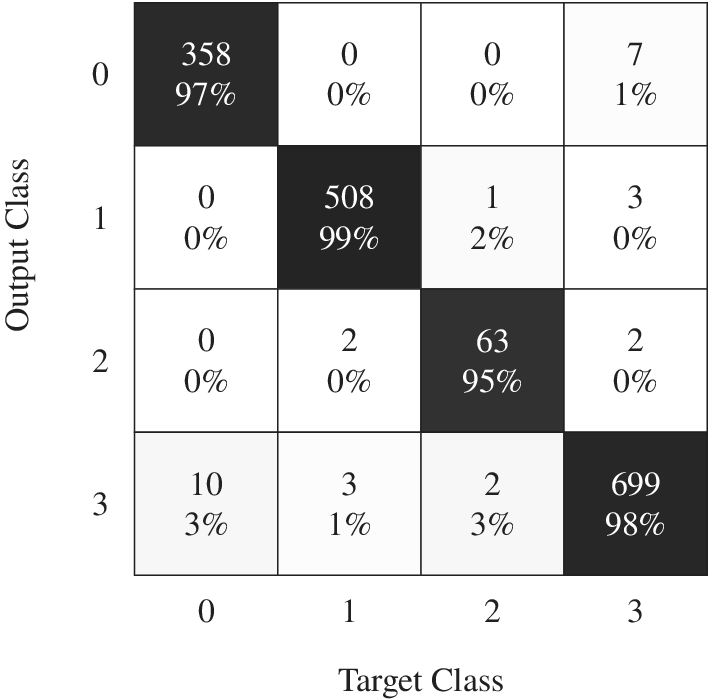
Figure A3. Confusion matrix for the FWANN classifying the states of the compressor for the test set: numerical error (0), functioning (1), surge (2) and choke (3). Given in thousands and rounded.
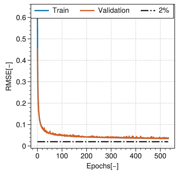
Figure A4. Evolution of RMSE in function of number of epochs for the FWANN predicting efficiency. Overfitting is avoided by interrupting the network training when the validation error starts increasing again. Training and validation converge towards a 4% asymptote after 500 epochs.

Figure A5. Evolution of RMSE in function of number of epochs for the FWANN predicting pressure ratio. Overfitting is avoided by interrupting the network training when the validation error starts increasing again. Training and validation converge towards a 1% asymptote after 500 epochs.


 Open access