


Background and Aims
The aim of this paper is to report further progress on a project to simulale the changes of the whole global climate system through the period of the ice ages, forced only by the variations in the external solar radiation regime associated with the Earth's orbital changes. Changes of the internal components of the global climate system, involving the atmosphere, ice and ocean, need to be prognostic. It is still not computationally possible to run a high-resolution complete global climate system model continuously through multiple ice-age Cycles. Therefore at this stage we use a hierarchy of models with asynchronous coupling to simulate the changes in a preliminary way and to carry out sensitivity studies of various components of the system.
Atmospheric sea-ice general circulation models (GCMs) and atmosphere-ocean-sea-ice GCMs can be used to com-pute “snapshot” climatologies at key epochs of the time series for climate change through the period, such as ihr Last Glaciol Maximum (LGM), the Last Interglaciol (LIG) and other stadiale, intersiadials or periods of rapid change. Global-climate energy-balance models (EBMs) are used, with certain features paramcteriscd from the GCMs, to run continuously through the ice-age cycles, coupled to icesheet models and driven by the external radiation variations from the orbital changes.
Ice-sheet models are chiven by the output from the FBMs but also feed back into the FBM the results of ihr ice-sheet changes. Because the ice-sheet changes are relatively slow it is found that the asynchronous coupling allow s this feedback to be carried out adequately at intervals of about 1000 years Buck! and Rayner, 1990). The Northern 1 lemisphere and Southern Hemisphere domains for ice cover are treated separately, connected only by the synchronous climate of the EBM and a common sea level with which they both interact, For the Antarctic ice sheet the forcing of changes conies primarily from the local orbital radiation variations plus ihr effects of the Northern Hemisphere ice-sheet changes which influence the Antarctic temperature and accumulation rate and the sea level.
Previous work by lincici and Smith (1981, 1987), who modelled the North American ice sheet in response io orbital forcing, found that although the summer radiation changes provided the crucial external driver of the ice-age changes, it was the internal feedback of the ice-sheet cover which dominated the time series for global mean temperature, it was found that a key requirement for the ice sheets to develop in the time available was for the orbital forcing to give rise to a temperature drop of about 4° C over summer near 70° Ν after the LIG. The ice-sheet rover at maximum provided additional temperature lowering in excess 5°C. To remove the ice sheets alter the LGM, the orbital forcing needed to provide the equivalent of about 6°C warming in the absence of ice sheets. Such equivalent warming lias been confirmed by GGM results (e.g. Reference MasonMason. 1979).
Investigations with annual-cycle orbital forcing and high-resolution topography, using a global EBM, by Budd and Rayner (1990, 1993) clarified the temperature changes resulting from the orbital changes alone and combined with the ice-sheet albedo effect. It was also found that the global annual mean temperature was negligibly influenced by the orbital radiation changes and was almost entirel) due to the ice-cover and associated changes, such as sea level, and possibly smaller in-phase effects including atmosphere composition.
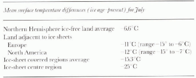
Λ further important result from the EBM with 1° latitude resolution was that there were very large and sharp gradients of surface summer temperature change near the edge of the ice sheets from about -30° over the ice sheet to about -6°C over land areas south of the ice sheets (cf. Budd and Rayner, 1990. Fig. 2).
Similar results were found at coarser resolution with the GCMs (e.g. Reference GatesGates, 1976a, b; Reference Manabe and BroccoliManabe and Broccoli, 1985; Reference RindRind, 1987). The strong influence of the ice sheet on the global temperature was also illustrateci by the GCMs, particularly those of higher resolution. The strength of this ice-sheet albedo feedback is dependent on the prescribed albedo, which is poorly known for the ice sheets and which could vary from near 0.9 for the high interior to 0.4 over the high ablation zone near the edge. This question lias been examined here by sensitivity tests to temperature forcing over the ablation zone at the edge of the ice sheet to derive the best-fit mean temperature drop at the LGM for the Northern Hemisphere appropriate for the ice-edge region.
Corresponding results from the GCM results of Gates (1976a, b) using the earlier CLIMAP (1976) data are shown in Table 1. These results are used in preference to those from the later CLIMAP data, due to the problems raised by many workers (e.g. Rind and Peteet, 1985; Reference Webb, Rind, Lehman, Healy and SigmanWebb and others, 1997).
Observational evidence for the large gradient in ice-age temperature differences from the land south of the ice edge to the interior was provided by Cuffey and others (1995) for the central ice-sheet region of Greenland, and by Reference Levesque, Cwynar and WalkerLevesque and others (1997) for the North American ice-margin region. Coupled modelling of the climate ice-sheet system for the Northern Hemisphere through the Glaciol cycle was also carried out by Reference Deblonde and PeltierDeblonde and Peltier (1991), Reference Huybrechts and T'siobbelHuybrechts and T'siobbel (1995). and Reference MarsiatMarsiat (1995). The present study also includes ice shelves and obtains a reasonable match to estimated LGM ice limits compiled from observations e.g. Reference Grosswald and HughesGrosswald and Hughes, 1995).
Table 1. Table 1. Differences in ice-age temperature cahnges across ice-edge regions from land to ice sheet (derived from dales, 1976a, b)
Outline of Modelling of the Northern Hemisphere Ice-Age Cycle
The domain for the Northern Hemisphere used here is taken from the North Pole to 30° Non a stereographic projection using a rectangular grid of 50 km based on the scale of 50° Ν latitude. This work is taken as preliminary for sensitivity tests before converting to a corresponding spherical-surface domain. The topography for land and seabed are taken from a data base of approximately 10 km spacing and averaged over the domain-scale gridpoints.
The ice-sheet model is similar to that used previously for the Antarctic by Budd and Jenssen 1989: and Budd and others (1994). Because of space limitations, only the most pertinent points are emphasised here. A detailed description of the model is given in Reference MavrakisMavrakis (1993).
The model includes a simplified ice-shelf formulation for rapid computation over arbitrary domains through the ice-age cycles. The model derives the loci of centre-line flows from surface-slope vectors and takes account of transverse and longitudinal stresses in a simplified manner where the ice shelf is bounded, or grounding points occur. At ice fronts the free-floating strain rate is used following Reference WeertmanWeertman's (1957) formulation (cf. Budd and others, 1987). A calving criterion is applied to the floating ice when the ice thickness reduces to below 250m. Although this formulation is crude compared to a complete two-dimensional stress-field model of the type developed by MacAveal and Thomas (1982), the present model provides a reasonable first-order representation of existing Antarctic large ice shelves in velocity, thickness and extent, and is also relatively rapid to compute for ice-age cycles. An initial basal melt rate for the Arctic Ocean of 0.2 m a−1 is applied and this is reduced during the ice age with lower sea level. For the Northern Hemisphere ice sheets, much of the basal zone in the low-elevation regions is found to be near pressure-melting point for most of the time, so the flow parameters for temperate ice from Budd and Jacka (1989) are used with sensitivity studies around these values for ice deformation and sliding. The deformation and sliding relations as outlined by Budd and Jenssen (1989) provide input to the continuity equation.
At the upper surface, the net accumulation is obtained from an initial distribution of precipitation (or net precipitation minus evaporation) plus an ablation rate based on mean summer temperature, following Budd and Smith (1987). The mean summer temperatures are taken from compilations of present surface temperature and decrease with height using a prescribed lapse rate of 6.5°C km−1. As the ice-sheet elevation increases, the net surface precipitation decreases, according to the “elevation-desert effect” described by Budd and Smith (1981).
A number of data sources for the present distribution of surface temperature and precipitation were used. These include Reference JaegerJaeger (1976), Melbourne University GCM and the European Centre for Medium-range Weather Forecasting Global Analysis Archives.
Sensitivity studies were carried out to examine the consequences of the relatively large differences between these datasets and to examine possible changes in precipitation for diflerem Glaciol epochs, based on the results of GCM modelling. Although large decreases in snow accumulation OGCUr over the ice-Covered areas during the Glaciol periods, the dominant changes are primarily covered by the elevation-desert effect.
A simple non-linear isostatic bed response formulation is used as given by Budd and Smith (1981) as follows:
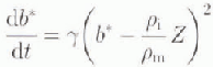
where b* is the bed elevation difference from equilibrium as a function of time (t) for an ice-thickness departure from equilibrium z with pi
and pm
the effective densities for ice and mantle, respectively. The constant ϒ used here has a value of 0.0005 km −1 a−1. The value of ![]() is taken as 3.3.
is taken as 3.3.
The present bed has been relaxed upwards by an amount corresponding to the residual depression remaining at the end of the simulation, reaching the present conditions following the ice-age cycle. The constants are chosen to match the total uplift since the ice age and the present uplift rate for the Hudson Bay region.
The temperature forcing through the ice-age cycle is taken from the EBM results of Budd and Rayner (1990) with combined radiation and ice-sheet albedo feedback. Because the temperature of the ablation zone was not well resolved by the EBM (or the GcMs), the magnitude of the temperature shift here was taken as an unknown scaling factor for that forcing, and a series of simulations was carried out to derive the best fit for the ice edge at LGM. A large number of additional simulations were carried out to test the sensitivities to the wide range of variables as described above. Only a few of the major results can be given here.
Results of the Northern Hemisphere Simulations
Figure 1 shows flow the maximum ice extent at LGM from the model changes with the magnitude of the maximum temperature drop at LGM (ΔT) in the marginal zone of the ice sheets for ΔΤ =-4,-8,-12,16 ° C. The results displayed are selected from a series with 1°C steps of ΔT and from a large number of sensitivity rims with variations in the precipitation and other parameters. The case for ![]() matches most closely the maximum extent from compilations of observations for the complete Northern Hemisphere (e.g. Denton and Hughes. 1981; Grosswald, 1988; Grosswald and Hughes. 195). Note that the steep marginal ablation zone for the ice sheets tends to be sub-grid scale for the GCMs and the EBM of Budd and Rayner 1990. The temperature shift of
matches most closely the maximum extent from compilations of observations for the complete Northern Hemisphere (e.g. Denton and Hughes. 1981; Grosswald, 1988; Grosswald and Hughes. 195). Note that the steep marginal ablation zone for the ice sheets tends to be sub-grid scale for the GCMs and the EBM of Budd and Rayner 1990. The temperature shift of ![]() for the ice edge resolves belter the change given by the EBM, going from -6°C over land to -30° C over the ice cap, and the similar results for the GCMs given in Table 1.
for the ice edge resolves belter the change given by the EBM, going from -6°C over land to -30° C over the ice cap, and the similar results for the GCMs given in Table 1.

Fig. 1.
Variation in the modelled LGM extent of ice for the North Polar region, shown as a Junction of maximum temperature lowering ![]() appropriate for the ice-edge region, lce-edge positions are shown by increasing areas in colour shading (from yellow to dark blue) for
appropriate for the ice-edge region, lce-edge positions are shown by increasing areas in colour shading (from yellow to dark blue) for ![]() . The calne of
. The calne of ![]() provides lite closest match to observational-based LGM reconstructions.
provides lite closest match to observational-based LGM reconstructions.

Fig. 2.
Distribution of ice thickness at LGM over the. Northern Hemisphere topography, shown for the model run with ![]() . The distribution of grounded and floating ice show considerable similarity to that of the paleteo-reconstruction of Grosswald and Hughes (1995). Contours for ice thickness are shown for 0, 1, 2, 3 km and for the land topography with colour boundaries 0, 0.3, 0.5. 1,2,3 km.
. The distribution of grounded and floating ice show considerable similarity to that of the paleteo-reconstruction of Grosswald and Hughes (1995). Contours for ice thickness are shown for 0, 1, 2, 3 km and for the land topography with colour boundaries 0, 0.3, 0.5. 1,2,3 km.
The temperature drop around the iee-edge region should not be expected to be uniform, and the results obtained here indicate that differences of ± 1°C in different locations could account for discrepancies in the maximum ice-edge positions. Similar eilects are found from variations of about ±20% in the local precipitation rate for a region. The pattern for the distribution of ice thickness at LGM for the case with ΔΤ = -12°C is shown in Figure 2. Quite close resemblance is seen with the Grosswald and Hughes (1995) compilation for extent, and the Grosswald (1988) reconstruction for ice thickness, although it is recognised that the representation of the extent of ice in Siberia at that time is still controversial.
Nevertheless it appears from the model that the development of marine ice sheets around the Arctic Islands and a floating ice shelf over the Arctic Ocean during the ice age would be a clear result of the cooling and lowered firn line. The pattern of flow of the ice shelf across the Arctic from Euro-Asia and North America to Fratti Strait, east of Greenland, resembles closely the pattern seen from apparent ice scour and iec-rafled debris by Reference Bischof and DarbyBischof and Darby (1997).
Figure 3 shows the corresponding distribut ion of ice over land at the end of the Glaciol-cycle simulation corresponding to the present. The distribution gives a reasonable representation of the present observed ice distribution and provides a useful test for the present climatic forcing for temperature and precipitation, as well as for the model. Some features, such as the Barnes Ice Cap on Ballin Island, are found to exist in the model for the present only as a result of the Glaciol cycle. This is bec ause the bedrock elevation is too low, without the ice coser, to form a positive net accumulation region under the present climatic conditions.
The pattern of temperature forcing and ice-volume response (for grounded ice, floating ice and the fraction of ice volume affecting sea-level change) is shown for the case given in Figures 2 and 3, together with the bed-depression volume for the ice-age cycle in Figure 4. The Northern Hemisphere ice-volume fraction associated with sea-level

Fig. 4.
Present-day ice cover on land produced by the model at the end of the run through the Glaciol cycle with ![]() , following the LGM of Figure 2. The Greenland ice sheet and Barnes Ice Cap remain from the Glaciol conditions. Continus for ice thickness and land elevation are the same as for Figure 2.
, following the LGM of Figure 2. The Greenland ice sheet and Barnes Ice Cap remain from the Glaciol conditions. Continus for ice thickness and land elevation are the same as for Figure 2.
change, when compensated for by the bed depression, and ocean-bed responses, agrees reasonably with estimates of low sea level at LGM without the need for an additional large Antarctic contribution. in fact, the results presented below indicate thai the Antarctic contribution to sea level for the bulk of the ice age is found to be negative, with a smaller ice-sheet volume but greater extent at LGM than at present.
Antarctic Ice Sheet and Forcing for the Glaciol Cycle
Initially, it is not known what the extent of disequilibrium is for the present Antarctic bedrock isostatic adjustment. The data for the model are based on the 20 km grid dataset described by Budd and Jenssen 1989. The ice-sheet temperatures and ice-flow parameters were based on the results for the steady stale for the present regime and the match between the computed surface velocities and observed velocities as given by Budd and Jenssen 1989). For the model simulations the procedure adopted is as follows. The ice is removed and the bed relaxed up to equilibrium. Then the ice sheet is simulated from a period prior to the Glaciol maximum which preceded the Last Interglaciol through to the present (approximately 150-0ka BP). The forcings for the icc-shcet changes are dislalie sea level (primarily resulting from the Northern Hemisphere ice changes), the net accumulation rate and the mean climatic temperature changes. The accumulation-rate changes are based on the results from the Vostok ice core given by Reference JouzelJouzel and others (1987) and Reference Lorius, Raisbeek, Jouzel, Raynaud, Oeschger and LangwayLorius and others (1989). It is assumed here that the broad changes in accumulation rate over the Antarctic continent were proportional to those at Vostok taken as a percentage change of the present accumulation rate. Additional changes to this base rate are derived from the changes in ice-sheet elevation above sea level as given by the elevation-desert formulation described above.
The temperature changes come from the FBM, using combined radiation and ice-sheet effects, and including the changes of the sea-ice extent, as described by Budd and Rayner (1990, 1993). Those results provide a close match to the Vostok δ18O proxy temperature record from Lorius and others (1985) and Jouzel and others (1987), more particularly for the winter season, over which most of the nel accumulalion occurs.

Fig. 4. Time series for the temperature forcing (far ΔTm= -12°C) from the combined orbital radiation changes and ice-sheet albedo feedback (bottom), together with the ice-volume responses (top). for total ice (purple), grounded ice (blue). ice Volume affecting sea level (red) and the volume of bedrock depression
These forcing changes were applied to simulate changes of the Antarctic ice sheet, from before the last interglaciol to the present, for a large number of runs to lest the model's sensitivity to adjustments to the magnitudes of the prescribed forcing and to uncertainties in the ice flow and sliding parameters used in the model. Some simulations have been run with the 20 km grid resolution, but because of the long computation time required a reclin ed 100 km grid has been used for a much larger number of sensitivity studies. It has been found thai the large-scale average changes are well simulated with the 100 km grid, but significant differences occur in the detail, particularly around the coast.
Results for the Antarctic Glaciol Cycle Simulation
In order to examine the relative influence of the different components of the forcing, the changes were simulated separately for the indiv idual factors, as well as in combination. The results show that the effect of eustatic sea-level changes alone resulted in ice grounding-line advance during the Glaciol periods particularly around the large ice shelves, with thickening in the interior and an increase in ice volume. By contrast, the changes in accumulation rate alone caused thinning of the ice sheet and a reduced ice flux at the edge. For the combined effects, the impaci of the reduced accumulation dominates for lite whole ice sheet, but regionally, particularly around the large ice shelves, the eustatic sea-level changes cause large c hanges in the area of grounded ice.
These results are illustrated by the ice-volume time series shown in Figure 5, giving separately the results for the changes of accumulation and sea level alone and then combining them. These results imply that the changes in Antarctic ice volume during the Glaciol cycle could have a small offset elicci on global sea-level changes produced by the Northern Hemisphere ice changes. The similar study by Huv brechls (1990, 1992) obtained a net increase in Antarctic ice volume at LGM. The dillercnccs between those

Fig. 5. Time series for Antarctic ice-volume changes (total, grounded and affecting sea level. as in Fig. 4) through the last Glaciol cycle from the model for the sparate forcing of accumulation changes, sea-level changes and combined accumulation and sea-level changes. It appears that The accumulation-change effects are dominant for the ice volume at LGM.

Fig. 6. The near to present (pre-industrial) state of balance of the Antarctic ice sheet (averaged over the last 2ka) is shown from the model (with 100km grid) after the end of the ice-age cycle to the present. The state of balance is expressed as the rate of change of ice thickness as a fractionof the present accumulation rate. The interior and in parts of West Antarctica slight thinning tends to predominate. The zero is shown bold, and the color scale for the small nagative values has been expanded.
results and the results obtained here appear to the due in several factors. These include the differenl forcings used for sea level and the accumulation-rale pattern. The formula-lion of ice sliding was also different and the models are particularly sensitive to the sliding relation and the values of the parameiers used in it. Finally, the differences in the ice-shelf models may also he an important factor in the different changes in ice thickness over the huge ice-shelf areas.
The model results presented here indicate that the simulated Antarctic ice-sheet margin at LGM was more advanced and thicker than for the present ice sheet, due to the lower sea level. At the same time, there was reduced thickness in the interior, particularly in Last Antarctica, clue to the lower accumulation rates. These characteristics together resulted in a slightly smaller net grounded ice volume than thai of the present ice sheet.
These results are still regarded as preliminary because the changes in West Antarctica, particularly in the region just inland of the large ice shelves, are very sensitive to the model flow and sliding parameters and to the past accumulation rates. Observations giving grounding-line positions al the LGM and past accumulation rates are particularly valuable in constraining the model results in this regard. Nevertheless the changes for East Antarctica appear to be reasonably robust, and so we next examine the implications of the model for the present stale of balance of tin- Antarctic ice sheet.
Assessment of the Current State of Balance and Rate of Change of the Antarctic Ice Sheet
The time series for ice-volume change of the Antarctic ice sheet from the model displayed in Figure 5 shows a rapid increase in volume after the LGM following the accumula-lion-rate increase. By about 8000 years ago t his rate of change had very much decreased as the ice approached the new state of balance with the Holocene climate. By the present, the ice-sheet model volume continues to increase by about 0.025 km−3 a−1, which is equivalent to only about 0.08 mm a−1 of sea-level lowering.
The distribution of the imbalance, however, is far from uniform, with the more slown responding interior of East Antarctica (particularly above 3000m) still building up, whereas the more coastal areas (primarily below 2000 m) are more nearly in balance, or even in slight negative balance, from the responses to sea-level change and the slower subsequent bedrock adjustment.
These features are illustrated in Figure 6 which shows the model results for the present rate of change of the ice sheet at the end of the ice-age simulation averaged over the last 2000 years expressed as a fraction of the present accumulation rate. The interior region of East Antarctica shows a positive balance generally between 5% and 20% but reaching 40% at dome summits. This positive-balance region extends to near the grounding line in the Lamben Glacier valley, a result which appears to be supported in observations in thai region (Allison, 1079; Reference Higham, Craven, Ruddell and AllisonHigham and others. 1997). Around the coastal regions generally, the imbalance values tend to be variable but typically less than ±5%.
In West Antarctica the large interior negative-balance regions are primarily related to the large grounding-line shilts due to the dislalie sea-level changes, It should be em-phasised that it appears from the ice-core data e.g. from Vostok, Byrd, Law Dome), as well as the modelling, that this gradual approach towards equilibrium has been taking place over many thousands of years through the Holocene, right up until the pre-industrial period, last century, before anthropogenic influences on climate may have become significant. The results presented by Smith and others 1998) indicate that since last century the effects of global warming appear to have been increasing the Antarctic net accumulation rates by up to 5-10% by the present. This recent increase towards a positive net balance for the present would need to be added to the post-ice-age long-term changes modelled here to give the stale of balance anil current rate of change of the Antarctic ice sheet for the present day.
Conclusions
It is apparent that the Northern Hemisphere ice changes through the Glaciol cycle can be reasonably well simulated from the orbital radiation changes plus the ice-sheet albedo feedback. This generates the global sea-level anil chinale changes that together with the local radiation changes drivi the Antarctic ice-sheet changes. The ice-core records provide additional information for the time changes of accumulation rates and temperature. The applied forcing resulis in an ice-age advance of the grounding line of the Antarctic ice sheet, with thickening around the edge, but with thinning in the interior due to the reduced accumulalion rate. A small volume decrease, equivalent to aboul 5 m of sea-level rise, occurs for the Antarctic model at the LGM relative to the present.
After the LGM the modelling- for Antarctic a gives retreat at the edge, from the rise in euslatic sea level, but thickening in the interior, from the increase in accumulation rate.
By the present century the model was close to the present ice-sheet configuration, giving a state close to overall balance and contributing only 0.08 mm a−1 to sea-level lowering. However, in the interior of East Antarctica there was still a net positive imbalance of about 20%, where the accumulation rate was low, and small negative balances of around 5% occurred in places around the coast, and of 5-10% over a large part of West Antarctica. It should be noted, however, that the derived rates of change for West Antarctica may not be so robust, even though the resulting configuration derived for the present is close to thai observed. Since last century the effects of global warming appear to have contributed an additional 5-10% towards a net positive balance (Smith and others, 1988), These resulis combined are in line with the recent mass-balance assessments by Budd and Warner (1996) giving above +30% positive balance over the inland region of Wilkes Land and under + 10% nearer the coast. The extension of the higher positive balance of the interior region down to Lambert Glacier is also well supported by the observations reported by Allison (1970) and Higham and others (1997).
Under a continuing global warming trend, resulting from increasing greenhouse gases, the positive balance inland can be expected to increase further until coastal basal melt and increased flow provide compensation (cf. O'Farrell and others. 1997:. The ice-sheet configuration Obtained here with slow regional changes of different sign, but near-zero overall nel balance, provides a reasonable starting-point (at pre-industrial times) for computing the Antarctic ice-sheet changes associated with global change, from last century to the present, and extending into the future.


