


INTRODUCTION
Knowing the absolute and relative date of different events within the sedimentary record is important for a wide variety of studies (e.g., Murray and Olley, Reference Murray and Olley2002; Ojala et al., Reference Ojala, Francus, Zolitschka, Besonen and Lamoureux2012). A range of techniques have been developed for this purpose, each having different benefits and limitations (e.g., Murray and Olley, Reference Murray and Olley2002; Appleby, Reference Appleby2008; Ojala et al., Reference Ojala, Francus, Zolitschka, Besonen and Lamoureux2012; Zolitschka et al., Reference Zolitschka, Francus, Ojala and Schimmelmann2015). Geochronology may, for instance, provide high accuracy point ages based on the dating of tephras (e.g., Naeser et al., Reference Naeser, Briggs, Obradovich, Izett, Self and Sparks1981; Miyairi et al., Reference Miyairi, Yoshida, Miyazaki, Matsuzaki and Kaneoka2004), organic material (e.g., Howarth et al., Reference Howarth, Fitzsimons, Jacobsen, Vandergoes and Norris2013; Richards and Britton, Reference Richards and Britton2020) or bedrock (e.g., Bierman and Caffee, Reference Bierman and Caffee2002), however individual analyses can be time consuming and expensive. Varve counting is an alternative, or complementary, technique that may be used where sediment shows a distinctive annual cycle.
These annual layers may be counted in the same way as tree rings or speleothem growth bands (Proctor et al., Reference Proctor, Baker, Barnes and Gilmour2000; Bunn, Reference Bunn2008; Ebert and Trauth, Reference Ebert and Trauth2015). Longer periodicity changes in climate may also result in periodic sediment changes: Mediterranean sapropels (Rohling, Reference Rohling1994; Cramp and O'Sullivan, Reference Cramp and O'Sullivan1999), Paleozoic cyclothems (e.g. Wanless and Weller, Reference Wanless and Weller1932; Heckel, Reference Heckel1977) and the Mesosoic Newark Basin sediments (Olsen, Reference Olsen1986) all record some form of the orbital (Milankovitch) cycles. Similarly, tidalites record changes in sediment deposition on the shorter tidal cycles (e.g., Kvale et al., Reference Kvale, Cutright, Bilodeau, Archer, Johnson and Pickett1995; Coughenour et al., Reference Coughenour, Archer and Lacovara2009). Just as tree rings result from differences in tree cell accumulation and growth rate throughout the annual climatic cycle (Schweingruber, Reference Schweingruber2012), any process that drives a change in sediment character with annual periodicity may generate a varve (DeGeer, Reference DeGeer1912; Zolitschka et al., Reference Zolitschka, Francus, Ojala and Schimmelmann2015). In both cases the theory is the same: a climatic cycle drives a change in the local sedimentation (or tree growth) dynamics, and this change is then recorded in the sediment (or wood) layers. Where this periodicity in sediment properties can be detected (i.e., where varves are present), it may be used to recover the original change in sediment dynamics. Where this change in forcing may reasonably be assumed to have an annual frequency, a chronology can be formed.
Conceptually, lakes may be thought of as filter functions (F[x(t)]), which receive for input a time varying climate signal (C(t)) and record depth varying sediment properties (S(z)). The climate signal reflects seasonal variations in temperature, precipitation, incoming solar radiation, and wind speed. Figure 1 provides an example of the real-world data associated with these terms. In the most basic form, we may write sediment properties as a function of climate:

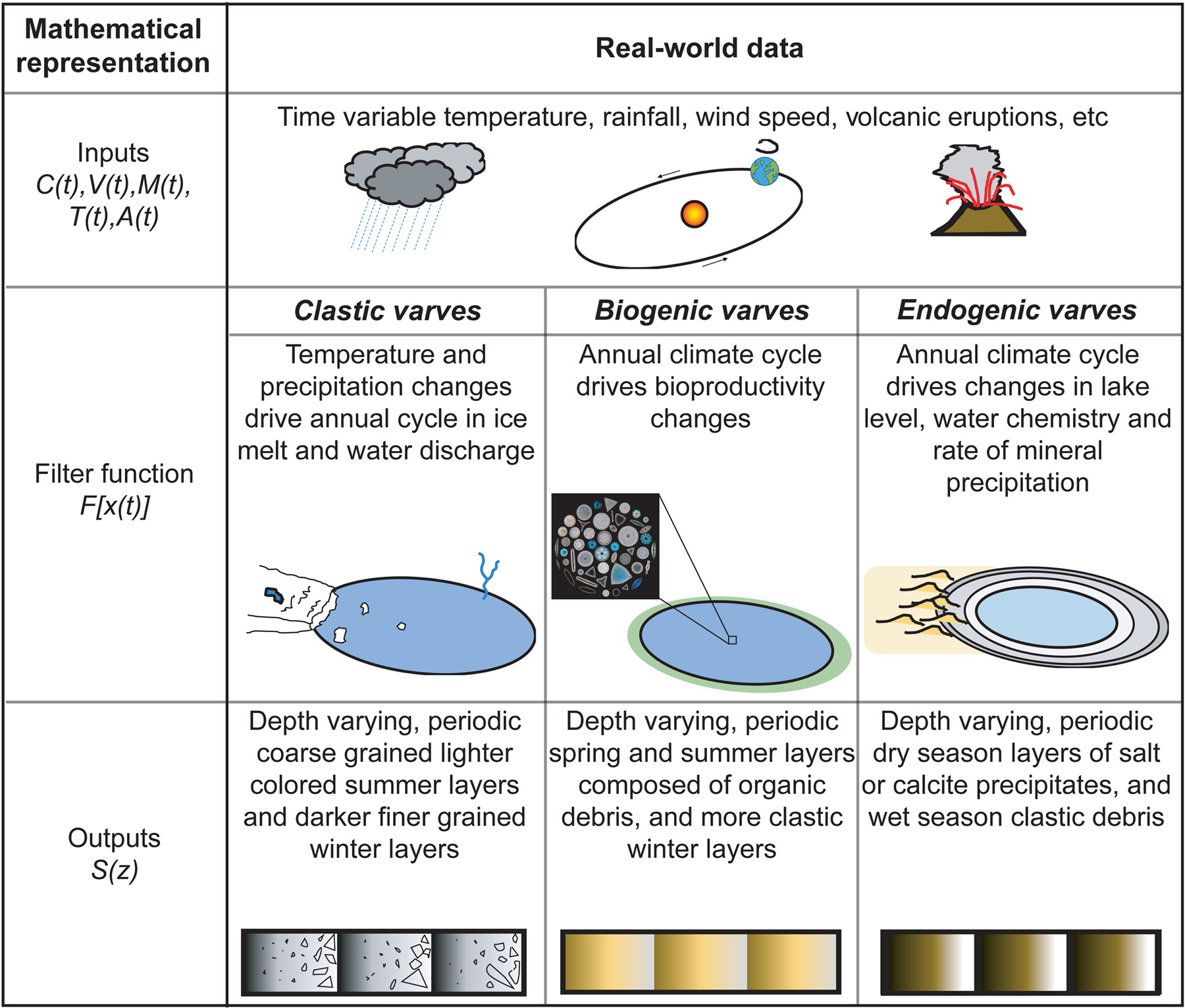
Figure 1. (color online) Conceptual model for the formation of three different end-member types of varves: clastic, biogenic and endogenic varves (Zolitschka et al., Reference Zolitschka, Francus, Ojala and Schimmelmann2015). This conceptual model may be described mathematically as a filter function, with depth-varying sediment properties as output.
Climate is often not the only parameter affecting sediment properties. Time-varying volcanism (V (t)), mass flows (M(t)), tectonics (T(t)), and anthropogenic activity (A(t)) among others may affect sediment deposition and characteristics. Sediment properties S(z) may then be written as a function of all these inputs:

The exact details of this filter function depend on lake location, geometry, bathymetry, and more, and will vary from lake to lake (and in some cases within a lake basin). For a sediment (S(z)) to be varved, two conditions must be met:
1. The input signal (C(t), V(t), M(t), T(t), A(t)) has an annual periodicity. In most cases this periodicity will come from the rainfall or temperature components of the climatic signal (seasonal variability), with the other inputs adding noise.
2. The specific filter function of the lake studied (F[x(t)]) preserves the periodicity of its input signal. The dimension of this periodicity is transformed from time (t) to depth (z). This is most commonly the case in seasonally (dimictic) or permanently (meromictic) stratified lakes (Saarnisto, Reference Saarnisto and Berglund1986; Larsen et al., Reference Larsen, Miller, Geirsdóttir and Thordarson2011; Zolitschka et al., Reference Zolitschka, Francus, Ojala and Schimmelmann2015). Lakes with a high depth-to-surface area ratio will have the best chance of preserving varves (Tylmann et al., Reference Tylmann, Szpakowska, Ohlendorf, Woszczyk and Zolitschka2012, Reference Tylmann, Zolitschka, Enters and Ohlendorf2013; Zolitschka et al., Reference Zolitschka, Francus, Ojala and Schimmelmann2015), as their sediment record is less likely to be disrupted by wind mixing and bioturbation. The formation of endogenic varves may be less sensitive to lake depth-to-surface area ratio (Last and Smol, Reference Last and Smol2001).
The development of quantitative transfer functions based on biological proxy records for physiochemical conditions is another example of how this concept may be applied (e.g., Anderson, Reference Anderson1995; Telford and Birks, Reference Telford and Birks2005; Birks et al., Reference Birks, Heiri, Seppä and Bjune2010; Saros et al., Reference Saros, Stone, Pederson, Slemmons, Spanbauer, Schliep, Cahl, Williamson and Engstrom2012; Juggins, Reference Juggins2013). Sedimentation rate changes may similarly be used to infer changes in past environmental conditions in certain circumstances (e.g., Bertrand et al., Reference Bertrand, Boes, Castiaux, Charlet, Urrutia, Espinoza, Lepoint, Charlier and Fagel2005; Larsen et al., Reference Larsen, Miller, Geirsdóttir and Thordarson2011). However, the specific filter function cannot generally be represented mathematically, and must instead be described via a conceptual model. Similarly, the exact forcings which result in annual sediment changes cannot always be determined; however, the resulting varves can be used to build a chronology.
Figure 1 shows an example of different conceptual models for endmember varve formation from a given set of inputs. Zolitschka et al. (Reference Zolitschka, Francus, Ojala and Schimmelmann2015) describe three main varve endmembers: clastic varves, biogenic varves, and endogenic varves. Clastic varves are the most common and are typically found in proglacial lakes (Carrivick and Tweed, Reference Carrivick and Tweed2013; Zolitschka et al., Reference Zolitschka, Francus, Ojala and Schimmelmann2015). In clastic varves, the filter function transforms the annual temperature and precipitation cycle into depth varying sediment grain size, mineralogy and colour. In some regions clastic varve chronologies have been extended more than 10,000 years into the past (Ojala et al., Reference Ojala, Francus, Zolitschka, Besonen and Lamoureux2012; Schlolaut et al., Reference Schlolaut, Marshall, Brauer, Nakagawa, Lamb, Staff and Bronk Ramsey2012, Reference Schlolaut, Staff, Brauer, Lamb, Marshall, Bronk Ramsey and Nakagawa2018). Biogenic varves will typically be found in lakes with a high primary productivity and strong annual temperature cycle. Spring and summer blooms of diatoms and other algae deposit layers of microfossils and organic material that are absent from winter layers (Smol and Stoermer, Reference Smol and Stoermer2010; Zolitschka et al., Reference Zolitschka, Francus, Ojala and Schimmelmann2015). Endogenic varves form in areas where chemically or biogenically induced mineral precipitation may be modulated by the annual climate cycle (Last and Smol, Reference Last and Smol2001; Zolitschka et al., Reference Zolitschka, Francus, Ojala and Schimmelmann2015). Alternatively, they may form from differential evaporite formation throughout the year, typically of salt (NaCl), aragonite (CaCO3) or gypsum (CaSO4⋅2H2O) (Zolitschka et al., Reference Zolitschka, Francus, Ojala and Schimmelmann2015). We note that while the above discussion focuses on lacustrine varves, annually laminated sediments may also be found in marine environments (e.g., Weber et al., Reference Weber, Reichelt, Kuhn, Pfeiffer, Korff, Thurow and Ricken2010; Schimmelmann et al., Reference Schimmelmann, Lange, Schieber, Francus, Ojala and Zolitschka2016). A full list of several hundred varve-related publications has been compiled by the Varves Working Group (accessible at: http://pastglobalchanges.org/science/end-aff/varves-wg/varve-related-publications).
The theory of varve chronology is simple, however counting any significant number of varves remains a time consuming and error-prone task. Annual variations in sediment property are rarely as simple as theory predicts. Many varves are ‘mixed’, or formed through a combination of the above processes, and layers are often blurred, poorly preserved or otherwise ambiguous. Similar to how trees may have missing or false rings, the varve record may be incomplete and missing varves may be impossible to detect. In addition, the different varve formation mechanisms described in the previous paragraph result in different varve appearances. This ambiguity leads to a measure of subjectivity and uncertainty in manual counts, and complicates the process of building automated, computer model-based varve counters. Three main approaches have been taken to varve counting, with each attempting to overcome these challenges in different ways.
Manual varve counting is the oldest method used to build varve chronologies, and predates modern computing (e.g., DeGeer, Reference DeGeer1912; Antevs, Reference Antevs1922, Reference Antevs1953; Ridge and Larsen, Reference Ridge and Larsen1990; Wohlfarth et al., Reference Wohlfarth, Björck, Possnert and Holmquist1998). It relies on a user, typically a paleolimnologist or other sedimentologist, making an expert judgement as to what constitutes an annual couplet and counting them throughout the entire sedimentary package. Varves may be manually counted either in marine or lake cores (e.g., Hardy et al., Reference Hardy, Bradley and Zolitschka1996; Breckenridge, Reference Breckenridge2007; Shapley et al., Reference Shapley, Finney, Kruger, Starrett and Rosen2019), or in sediment exposures of various types (e.g., Trauth et al., Reference Trauth, Alonso, Haselton, Hermanns and Strecker2000). A number of studies have been conducted analysing the accuracy of manual counts, and have found that even for intact sediments, counts may differ by more than 10% from externally constrained ages (Sprowl, Reference Sprowl, Bradbury and Dean1993; Aardsma, Reference Aardsma1996; Tian et al., Reference Tian, Brown and Hu2005). Repeated counts and counts by multiple different specialists improve the precision and accuracy of resulting chronologies, but are time consuming (Tian et al., Reference Tian, Brown and Hu2005). In addition to these limitations, manual recovery of depth varying sedimentation rates is a time consuming task. The clear limitations of manual varve counting, combined with recent improvements in both computer processing power and digital imaging technology, have resulted in attempts to automate the varve counting process partially or fully.
Early attempts to automate varve counting were often based on the simplifying assumption of summer sediment layers as light coloured as opposed to dark coloured winter sediment layers. This assumption is often valid in glacial lake environments where a high flow regime in spring and summer flow deposits coarser, lighter coloured sediment, while a lower flow regime in the winter allows finer, darker silts and muds to settle out (Weber et al., Reference Weber, Reichelt, Kuhn, Pfeiffer, Korff, Thurow and Ricken2010; Ebert and Trauth, Reference Ebert and Trauth2015; Zolitschka et al., Reference Zolitschka, Francus, Ojala and Schimmelmann2015). Digital core scans or images may then be converted to grayscale images, and the number of light and dark layers counted along a given transect using a peak-finding algorithm (e.g., Ripepe et al., Reference Ripepe, Roberts and Fischer1991; Francus et al., Reference Francus, Keimig and Besonen2002; Zolitschka et al., Reference Zolitschka, Mackay, Battarbee, Birks and Oldfield2003; Meyer et al., Reference Meyer, Faber and Spötl2006; Lewis et al., Reference Lewis, Francus, Bradley and Kanamaru2010). The number of peaks within the transect corresponds to the number of lighter coloured summer layers, and the number of troughs corresponds to the number of darker winter layers. Various adaptations of this simple idea have been used, including the counting of peaks along multiple transects and the use of curvature to detect the transition from peak to trough. Various easy-to-use tools are available to count varves in this manner, with BMPix and PEAK being the most recent and widely used (Weber et al., Reference Weber, Reichelt, Kuhn, Pfeiffer, Korff, Thurow and Ricken2010). Intensity transects may also be extracted from micro-XRF and X-radiography (Marshall et al., Reference Marshall, Schlolaut, Nakagawa, Lamb, Brauer, Staff and Ramsey2012), or from thin sections (Brauer, Reference Brauer, Fischer, Kumke, Lohmann, Flöser, Miller, von Storch and Negendank2004). Automated transect peak intensity counting methods are extremely sensitive to impurities, image artefacts, and varves differing from the ‘ideal varve’ model, and may result in false positive varve counts. Being one dimensional measurements, they cannot account for lateral complexity in the sediment. Finally, counting techniques based on intensity variation developed for high sedimentation rate, alternating dark–light clastic varves may not work in other more complex settings such as biogenic varves.
Over the last 10 years, a new generation of automated varve counting software has emerged based on more complex machine learning techniques. Three approaches have been taken: one (Strati-signal) based on a K-nearest neighbour algorithm (Ndiaye et al., Reference Ndiaye, Davaud, Ariztegui and Fall2012), one based on an adaptive fuzzy logic inference system (Ebert and Trauth, Reference Ebert and Trauth2015) and one (DeepVarveNet) based on convolutional neural network algorithms (Fabijanska, Reference Fabijańska2019; Fabijanska et al., Reference Fabijańska, Feder and Ridge2020). In the first two, a representative selection of sedimentary facies must be interactively selected by the user for each varve sequence image in order to train the model and improve the number of correct varve matches along a transect of the core. In the latter, the convolutional neural network is instead trained on an external dataset and attempts to identify full two-dimensional varve boundaries. In all cases the results of the varve count are strongly dependent on the quality and quantity of training data. DeepVarveNet is the closest to fully automated varve counting, requiring little user input after initial training. It is, however, computationally expensive, and unlikely to produce optimal results with varves differing much from the training dataset which consists of cm-scale glacial lake varves (Fabijanska et al., Reference Fabijańska, Feder and Ridge2020). One additional limitation of machine learning techniques is that the computational methods are complex and understanding the models’ built-in structural uncertainties can take considerable time investment for non-specialist users.
In this study, we propose a new varve counting method based on image autocorrelation (Van Wyk de Vries et al., Reference de Vries, Ito, Shapley and Brignone2020). In the following section we describe the basic structure of the countMYvarves model, and how it differs from previous algorithms.
METHODS AND MODEL SET-UP
Image cross-correlation and auto-correlation are versatile image analysis techniques that have been applied to a range of scientific problems, from computer vision to fluid dynamics. Image correlation is routinely used across the Earth sciences, for example, to measure water turbulence and flow (e.g., Patalano et al., Reference Patalano, García and Rodríguez2017), monitor slope stability (e.g., Baba and Peth, Reference Baba and Peth2012) and calculate glacier surface velocities (e.g., Heid and Kääb, Reference Heid and Kääb2012; Millan et al., Reference Millan, Mouginot, Rabatel, Jeong, Cusicanqui, Derkacheva and Chekki2019). In its most basic form, image correlation is a mathematical operation which measures the similarity between two images. Two identical images will have a correlation coefficient of 1, two completely opposite images (e.g., photo negatives) will have a correlation coefficient of -1, and two unrelated images will have a correlation coefficient of approximately 0. Figure 2 shows a graphical example of the outcome of two-dimensional (2D) cross correlation.

Figure 2. Schematic example of two-dimensional cross correlation coefficients of different images. corr2d represents the two-dimensional cross correlation operation. Note how an identical image (B) results in a correlation coefficient of 1, a perfectly anti-correlated image (C) results in a correlation coefficient of -1 and an unrelated image results (D) in a null correlation coefficient. Varves are self-similar, thus comparing one varve to the next should result in a positive correlation coefficient.
In countMYvarves, raw core scans are first loaded into the program, converted into numerical matrices of colour intensity by summing the RGB bands, and pre-processed to reduce image noise. First, outlier pixel values in the image are detected using a median filter, and individual pixel values more than 20% off the local median are discarded. Secondly, any voids created by the previous step filled via linear interpolation. Finally, the raw core image is smoothed on a scale equal to one-third of the initial estimate of sedimentation rate. This step is necessary to smooth out excess noise that may be present in images but may bias results if the initial estimate of sedimentation rate is too far from the real value. countMYvarves includes a function that detects where an incorrect initial guess of sedimentation rates may have biased count results and writes a warning to the final report if it is the case. Results are not sensitive to small deviations (within 50% from the correct value). For high resolution scans or very large varves, the raw images may be re-sampled to a lower resolution to reduce computation times. The core image is then split up into overlapping segments (12 by default), each running the full length of the core. This has the advantage of providing multiple independent counts from each individual core to evaluate counting uncertainty. Due to each segment being independent of the others, the process may be parallelised (run on multiple computer processor cores simultaneously), resulting in a two- to three-fold reduction in computation time on a 6 core laptop (Dell XPS 15, 2×16GB DDR4 2666 MHz memory, 6-core Intel i7-8750H 2.20 GHz processor). The sliding-window autocorrelation algorithm is then run on each image segment. This calculates the two-dimensional correlation coefficient between a reference chip (spanning one varve) and a search region (about 15 varves in either direction). Calculations are carried out using a sliding window through the search region: a region of the same size as the reference chip is cropped out (the ‘correlation chip’), and convolved with the search region to calculate a two-dimensional correlation coefficient. The resulting one-dimensional correlation coefficient series is saved, and then the next down-core ‘correlation chip’ is extracted and compared (see Fig. 3).


Figure 3. Example of the varve counting workflow for core 12A from Lago Argentino. The raw core scans (a) are converted into two-dimentional pixel intensity maps (b), smoothed (c), and then correlated using a sliding window to calculate the depth-varying correlation coefficient plot (d). Note the unusually thick and bright varve denoted by a purple arrow, which is less similar to the other varves and thus results in a lower amplitude correlation peak. (For interpretation of the references to color in this figure legend, the reader is referred to the web version of this article.)
Equation 3 describes the key autocorrelation calculation. A mn and B mn represent the individual intensity values for each pixel in images A and B, and $\bar{A}$ and $\bar{B}$
 represent the mean pixel intensities for the same two images. In the numerator, each individual pixel value has the mean subtracted from it, and is multiplied with the result of the corresponding pixel from the other image; these values are then summed across the entire image. If the ‘bright’ (values much higher than the mean) and ‘dark’ (values much lower than the mean) parts of each image align, then they will be multiplied together and result in a high correlation value. If they are out of phase (e.g., if the high values in A correspond to low values in B) then they will result in a strongly negative correlation value. If there is no trend between the values in A and B then the summed terms will on average cancel out, and result in a correlation value close to zero.
Two-dimensional correlation coefficients are calculated in countMYvarves using MATLAB®'s corr2 function. For two m×n matrices A and B, this function calculates the correlation coefficient C 2D using Equation 3. A search region of 15 varves reduces the chance of the search being over-extended into a different sedimentation regime, while ensuring that at least 10 correlation estimates are stacked at each location. If the assumption of smoothly varying sedimentation is not met and varves within the search window are not entirely self-similar, then the signal-to-noise ratio of the final correlation estimate will be lower. Figure 4 shows an example of how this two-dimensional autocorrelation coefficient is similar to raw intensity transects for a ‘clean’ varve sequence, but provides a much more reliable result in the case of more ‘noisy’ varves.

Figure 4. Schematic example of varve counting with the intensity transect and autocorrelation methods. The blue and red lines represent two intensity transects, while the purple dashed line represents a cross correlation series of the same core. Examples are shown for a ‘clean’ varve sequence with a complete, undisturbed varve sequence (alternating dark and light varves, left), and a ‘noisy’ sequence with incomplete, missing, faded and otherwise complex varves (right). Both techniques result in reasonably good results for ‘clean’ varve sequences, but intensity transect counting introduces many artefacts for ‘noisy’ sequences. The amplitude of the two-dimensional correlation coefficient is reduced where noise is introduced, however the periodic varve pattern is still detected, and lateral heterogeneity can be accounted for. Autocorrelation is better able to discard information from holes in cores, dropstones, biogenic detritus and other non-varved materials. (For interpretation of the references to color in this figure legend, the reader is referred to the web version of this article.)
Once the sliding window has compared every ‘correlation chip’ within the search region to the reference chip, a trough-finding algorithm is run on the resulting correlation coefficient sequence to identify the next varve in the sequence (equivalent to the distance from the first correlation trough to the second correlation trough in the correlation coefficient sequence). This subsequent varve is taken as the new reference chip, and as such the calculations above are repeated for each varve in the core.
This results in approximately 15 correlation estimates for each point in the core, which are averaged. The resulting mean correlation sequence spans the entire length of the core and contains a peak at each location where the local sequence is correlated with neighbouring varves (centred on a varve), a trough where it is anti-correlated with neighbouring varves (i.e., where it is out of phase with a varve) and correlation coefficients close to zero where the region is largely unrelated to its neighbouring region (e.g., disrupted sediments, tephra layers, etc.) as described in Equation 3. The peaks and troughs are then counted in this core-wide mean correlation sequence, with the distance between subsequent peaks or troughs providing the sedimentation rate. Figure 3 shows an example of a smoothed and unsmoothed two-dimensional pixel intensity map, as well as the resulting correlation coefficient trend. One varve, denoted with an arrow, is an outlier with a higher thickness and pixel intensity than the others. The resulting correlation peak is smaller and broader, and this varve is still detected.
The resulting sedimentation rate plot is then post-processed in two steps: first with an automatic outlier detection algorithm, and secondly with an exclusion and interpolation algorithm. In the inputs step, countMYvarves users may select whether the assumption of smoothly varying sedimentation rate is justifiable in the given core. If so, the automatic outlier detection and correction algorithm finds mis-counted peaks and corrects them according to the local 10-year mean sedimentation rate. Where the model-derived sedimentation rate in a given ‘year’ is within 25% of double or triple the local 10-year mean, it is considered as two or three years of sedimentation, respectively. Similarly, where the model-derived sedimentation rate in two subsequent ‘years’ is more than 25% lower than the local 10-year mean, but the sum of the sedimentation rates for the two ‘years’ is within 25% of the local 10-year mean they are considered to have both been deposited in one single year. These assumptions are recorded and saved in the automatically generated outputs report and may be modified in the inputs if not justified.
The exclusion and interpolation algorithm is intended for use on areas where automatic varve counting is not possible. Such scenarios include sediment known to be missing (e.g., at the top of cores), disrupted or mixed (e.g., seismites, bioturbated layers), or layers deposited instantly (e.g., tephras, landslide deposits). If any such regions are present within the core scan image, the user must fill in an ‘excluded intervals’ Microsoft Excel® or LibreOffice Calc™ spreadsheet prior to running the code. In this spreadsheet the upper and lower bounds of each interpolated interval are entered, along with the choice of either interpolating the mean sedimentation rate across the interval (disrupted or missing sediment) or excluding the interval from the count (instantaneously deposited). Calculating sedimentation rate rather than simply measuring varve boundaries makes it possible to include portions of the core in the chronology for which no varves are visible. A notes column is also included in the excluded intervals spreadsheet to record a justification for each exclusion or interpolation. This spreadsheet is also written to the final outputs report. An excluded interval file template is provided within the toolbox download package (Van Wyk de Vries et al., Reference de Vries, Ito, Shapley and Brignone2020).
As a final step, countMYvarves automatically generates a sedimentation rate and age-depth plot for the given core section. These are saved to a dedicated outputs folder, alongside a .csv spreadsheet file of age and sedimentation rate with depth which may easily be loaded into various core visualisation programs. In addition, a short MS Word® outputs report is automatically generated (using a MS Office ActiveX macro on Windows, or MATLAB ‘print’ function on macOS and Linux). This report automatically loads the plots and describes the mean and variation in core age and sedimentation rate. The outputs report also includes a full account of the different model-based and user-defined assumptions involved in the automatic varve counting run. Portions of this document may easily be built into technical reports or scientific papers, and the full record ensures easy reproducibility and cross examination with other counts or dating techniques. Assumptions may easily be modified or relaxed with small changes to the run inputs, and can help narrow the focus of follow-up work. In the following section we will examine the results of different core chronologies calculated using countMYvarves.
RESULTS AND EXAMPLES
To evaluate the performance of countMYvarves, we compare the model results against manually counted and otherwise age-constrained cores. We use two widely different lakes and varve characteristics: landslide dammed Herd Lake in Idaho, USA (44.088°N, 114.175°W) and proglacial Lago Argentino in Southern Patagonia, Argentina (50.214°S, 72.453°W). Herd Lake has an area of less than 0.1 km2 with 0.5–1 cm scale biogenic varves while Lago Argentino has an area over 1000 km2 and mm scale glacial/clastic varves.
Herd Lake core
Herd Lake is a landslide dammed lake located in the Salmon River basin, Idaho, USA. This lake exhibits very high productivity and sedimentation rates (Shapley et al., Reference Shapley, Finney, Kruger, Starrett and Rosen2019). A strong annual cycle in diatom productivity results in distinct summer and winter sediment properties, with summer bloom cycles generating nearly pure diatom ooze of unusual annual thickness. These cycles may be counted as with any other varves. A sediment deposition chronology in this location is useful for examining how the biological and chemical environment in the lake has evolved since formation. An 11-m long sediment core was extracted from Herd Lake in 2013, spanning the entire lake history. The upper 8 m of this core are persistently laminated except where locally interrupted by ca. 1- to 15-cm thick graded event deposits. Based on sediment composition, coherence between couplet counts and 210Pb and 14C dating, and modern diatom ecology, the laminated sediment is interpreted as varved (Shapley et al., Reference Shapley, Finney, Kruger, Starrett and Rosen2019).
Figure 5 shows the results of four separate manual counts of these cores performed by different researchers, and the results from countMYvarves. There is a good match between full laminated core section age (1462 [+172 -148] years) derived from countMYvarves, and four separate manual counts (1466, 1470, 1503 and 1566 years). These ages are also consistent with a shallow 210Pb date and extrapolation to a basal 14C date (2450 ± 30 14C years at 11 m depth, in unlaminated sediment). In addition to providing a full core age, the model results provide an estimated age at each point along the core depth, allowing easier comparison if external data is available. For example, an age estimate may be derived for the thick dark sediment package located in the upper portion of section 5 [698 (+84 -69) years] and compared to externally derived ages if available. In addition to a core chronology, countMYvarves can provide a full record of changes in sedimentation rate in this location over the past 1500 years with no additional user input required. The counting of multiple segments provides both a median sedimentation rate and a quantified uncertainty (typically given as an interquartile range). This suggests that Herd Lake's primary productivity-controlled sedimentation rate has remained relatively steady at 4–6 mm per year for the last 1500 years, with a slight reduction in linear sedimentation rate with depth, and some thicker intervals at 8–10 mm per year. The apparent reduction in accumulation rate with depth may reflect increased compaction, which would be reflected in an associated increase in sediment density with depth.
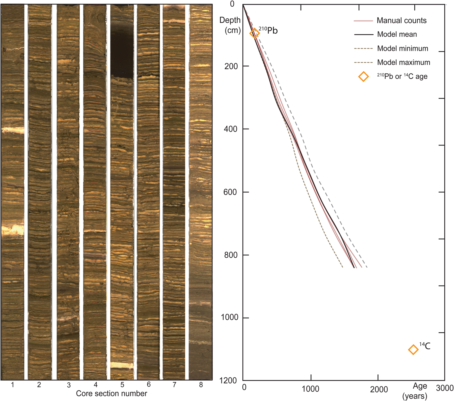
Figure 5. (color online) Results of automated varve counting of the Herd Lake, Idaho cores (left) and core scans (right; section 1 represents the core top). The results of the model and four separate full manual counts of the entire core are shown (right). Model core age [1462 (+172 -148) years] matches up well with manual counts (1466, 1470, 1503 and 1566 years). Manual counts were conducted by MV, MS, GB and EI. Age model modified from manual count, 210Pb, and 14C by Shapley et al. (Reference Shapley, Finney, Kruger, Starrett and Rosen2019).
Lago Argentino cores
Previous varve counting toolboxes have generally had good success counting large cm-scale varves, but have had considerable difficulty with varves smaller than 5–10 mm. In order to evaluate the ability of countMYvarves to resolve very fine scale laminations, we use an example from Lago Argentino, a large proglacial lake in southern Patagonia, Argentina (Skvarca and Naruse, Reference Skvarca and Naruse1997; Pasquini and Depetris, Reference Pasquini and Depetris2011; Richter et al., Reference Richter, Marderwald, Hormaechea, Mendoza, Perdomo, Connon, Scheinert, Horwath and Dietrich2016). Three large outlets of the Southern Patagonian Icefield (Glaciar Upsala, Spegazzini and Perito-Moreno) calve directly into this lake, resulting in a large influx of freshly eroded glacial flour (Skvarca et al., Reference Skvarca, Angelis, Naruse, Warren and Aniya2002, Reference Skvarca, Raup and Angelis2003; Pasquini and Depetris, Reference Pasquini and Depetris2011; Strelin et al., Reference Strelin, Kaplan, Vandergoes, Denton and Schaefer2014). The main basin of the lake is separated from these actively calving glaciers by a network of glacial fjords nearly 50 km long, and sedimentation rate in the main basin is dominated by gradual fallout of fine silt to mud-scale particles. Gravity core GCO-LARG19-12A-1G-1 (Fig. 6) is located in the centre west of the main lake basin, nearly 75 km from the nearest source of glacial sediment. Sedimentation rate is on the order of one mm per year, and clay-sized particles are dominant. Despite the distance from the glacial front, the sediment exhibits alternating mm scale light and dark layers. The 0.2 mm resolution XRF scans and lamina scale grain size analysis shows that the dark layers are coarser grained and more Ca-rich, whereas the light layers are finer grained and more K-rich. The periodic variation in sediment properties strongly suggests that these changes are driven by the seasonal cycle, and that they are varves. This also suggests that the Lago Argentino colouring is inverted relative to the classic clastic varve model, with light layers corresponding to winter deposition and dark layers to higher summer sediment supply.

Figure 6. (color online) Results of automated varve counting for a gravity core taken from the main basin of Lago Argentino, Argentina. Panels a and b show the raw core image and zones counted, extrapolated and excluded by countMYvarves. Panels c and d present the core sedimentation rate record, and age-depth model (including uncertainties). Model core basal age (258 +15 -13 years) matches up with the results of four independent manual counts (210, 235, 244 and 257 years).
Four different researchers (Maximillian de Vries, Mark Shapley, Guido Brignone and Emi Ito) conducted one or more independent manual counts of this core to provide a reference point for model runs. Where multiple counts were conducted by the same operator, results are averaged. The results of these manual counts have considerable spread (210, 235, 244 and 257 years), highlighting the limitations of manual varve counting in complex cores. The model core age (258 +15 -13 years) comes out as slightly higher, but largely consistent with manual counts. CountMYvarves was able to extrapolate counts over portions of the core (orange regions in Fig. 6b) that cannot be manually counted, so model basal age is expected to be higher by a small margin. Figure 6d shows the chronology results for each of the 12 overlapping segments of this core. The internal variability provides an estimate of the uncertainty of the mean age. Figure 6c shows the down core instantaneous sedimentation rate in this core. This shows a steady sedimentation rate in the 1–2 mm per year range, exhibiting a slight decrease from a peak of 2 mm per year at 200 varve years to around 1 mm per year today. This decrease in sedimentation rate may reflect the more than 10 km retreat of the nearby Upsala glacier since the end of the Little Ice Age 150 years ago. The top 20 mm of the core was slightly disrupted during coring, and as a result the decision was taken to interpolate over this disrupted portion using the average sedimentation rate. Manual examination of the sedimentation rate plot suggests that the actual sedimentation rate in this portion may in fact be slightly lower than this average. Core 12A does not appear to contain any tephra layers. However, other longer cores from the same lake contain thick tephra units more than 50 times the local varve thickness. If not accounted for, this would result in biased or incorrect bulk sedimentation rate and age results. CountMYvarves allows these layers to easily be marked as non-varved and excluded from the chronology. In addition, all such decisions are recorded in the outputs file and the assumptions may be modified if new information becomes available (for example if a layer that had been assumed to be disrupted sediment is determined to be a mass movement deposit).
DISCUSSION
To the authors’ knowledge, countMYvarves is the first tool to use image autocorrelation in the identification of varves. Image autocorrelation is ideally suited to this task for several reasons:
a) Autocorrelation can evaluate the two-dimensional shape of varves, and yield accurate counts even for deformed, sheared, or partially erased varves.
b) Autocorrelation is self-contained and identifies varves using only the characteristics of neighbouring sediment layers. Unlike machine learning techniques, it does not require training using an external dataset (Fabijanska et al., Reference Fabijańska, Feder and Ridge2020) or user inputs (Ndiaye et al., Reference Ndiaye, Davaud, Ariztegui and Fall2012; Ebert and Trauth, Reference Ebert and Trauth2015). This improves usability, reproducibility, and reduces the probability of bias from a non-representative training set.
c) Autocorrelation is scale invariant and may be equally successful on multi-cm scale varves as on mm scale varves.
d) Autocorrelation is insensitive to the colouring, scale and complexity of the repeated pattern. It is equally successful at detecting alternating dark and light clastic varves as at detecting more complex biogenic varves.
CountMYvarves also differs in approach with respect to previous automated varve counting techniques on two other points. Firstly, countMYvarves focuses less on recording of varve boundaries, and more on calculating sedimentation rates, equal to the derivative of varve thickness over time. Indeed, the thickness of a varve T v may be thought of as the integral of the sedimentation rate S with time:

with x in years. Since depth z is a known quantity, S may be converted to relative deposition age t d at a given depth z = d as follows:

Calculating a chronology from sedimentation rate S rather than varve boundaries enables extrapolation across areas of disrupted or missing sediment.
Secondly, countMYvarves does not attempt to fully automate the varve counting process. In most cases, a fully automated model will not be able to capture the full variability of sediment styles or account for preservation and coring artefacts. Attempts to fully automate the process may result in complex assumptions built into the model structure, and results that are difficult to reproduce or interpret. Semi-automated varve counting can not only help speed up the counting process, but also improves the transparency and reproducibility of results. CountMYvarves simultaneously performs autocorrelation along multiple segments of the core similar to how multiple users may perform repeated manual counts, which allows for the quantification of uncertainty in both depth-varying ages and sedimentation rates. This facilitates more robust comparison of core ages with other dating techniques (e.g., radiocarbon) for which uncertainty analysis workflows are well established.
Figure 7 provides a breakdown of the advantages and limitations of different varve counting methods. Partially automated varve counting remains challenging, but countMYvarves bridges some of these issues and provides a platform to perform rapid and reproducible varve counts on cores. User input is still required to select which regions of a core are expected to contain varves and which do not, but the counting process is fully automated. Ojala et al. (Reference Ojala, Francus, Zolitschka, Besonen and Lamoureux2012) suggest that greater digital documentation of varve counts is critical for increasing the scrutability and intercomparability of studies. To this end, countMYvarves automatically generates a short 3–4 page report for each core section run. This report highlights the assumptions that were made while calculating the results and warns users if any input parameter may have biased these results. This digital record may be used by subsequent users to easily reproduce the same run, adjust the assumptions and input parameters according to new information, or compare the results to those from a different lake.

Figure 7. Summary of the advantages and limitations of different varve counting techniques.
CONCLUSIONS
CountMYvarves is an open source, interface-based, semi-automated varve counting toolbox. We provide comparisons between model varve counts and multiple manual counts to validate the model set-up. CountMYvarves successfully reproduces manual count results for both complex biogenic varves (e.g., Herd Lake cores), and very low sedimentation rate cores (e.g., Lago Argentino cores). CountMYvarves uses two-dimensional autocorrelation to detect repeated patterns in a digital core scan, counts the number of repeated patterns and converts this to sedimentation rate. We then integrate this sedimentation rate over depth to provide an age-depth model. Varves are simultaneously counted along multiple two-dimensional strips of the core, allowing calculation of both the median and uncertainty in sedimentation rate and age at each depth point. In addition to automating the varve counting and uncertainty quantification procedure, countMYvarves also automatically generates a lab report and figures for each core section. CountMYvarves for Windows, macOS and Linux may be downloaded at: https://doi.org/10.5281/zenodo.4031811.
Acknowledgments
Maximillian Van Wyk de Vries was supported by a University of Minnesota College of Science and Engineering fellowship. We acknowledge the critical role played by the logistical and design expertise of Ryan O'Grady and Anders Noren of the Continental Scientific Drilling Facility (CSDF) in all planning and field phases of this research. Kristina Brady Shannon, Jessica Heck, Alex Stone and Rob Brown seamlessly coordinated core processing and analytical activities at CSDF. We thank Matias Romero, Anastasia Fedotova, Cristina San Martín, Guillermo Tamburini-Beliveau, Alexander Schmies and Shanti Penprase for their help with core recovery or processing, and all Spanish-speaking team members for their critical contribution of language skills. We particularly thank capitán Alejandro Jaimes for his expert ship handling under challenging conditions, and for sharing his incisive knowledge of Lago Argentino during the coring cruise. Finally, we would like to thank editor Peter Langdon and reviewers Jack Ridge and Arndt Schimmelmann for insightful comments and suggestions.
Financial Support
This work is supported by the National Science Foundation under Grant No. EAR-1714614, coordinated by Lead PI Maria Beatrice Magnani.


 Open access