Introduction
In an earlier paper (Reference HoldsworthHoldsworth 1974), longitudinal strain-rates were derived for Erebus Glacier Tongue (EGT) (Fig.l) using the velocity gradient obtained from a plot of ice-flow rate versus distance along the tongue. The points on this curve were obtained from the change in position of a set of marginal “teeth” which appear in successive aerial photographs taken between 1947 and 1970 (Fig.2). The accuracy of the flow-rate determinations depended primarily on the accuracy of the mapping and the reliability of point identification. It was possible to show, using these data, that the flow law “constants” derived, were only in fair agreement with previously published results (Reference ThomasThomas1971). Due to a scale error in the 1970 map, the height of the glacier surface above sea-level was everywhere up to about 10% too large. Although the flow rates are also correspondingly larger than they should be, the strain-rates derived from them are not significantly changed by this error. Because the freeboard of the glacier is less than previously assumed, the calculated effective stresses now differ from those previously given. Furthermore, it is evident that the effective shear stresses given in Reference HoldsworthHoldsworth (1974) are too low due to a truncation error in the numerical integration. The result now is to give a closer agreement with the data of Reference ThomasThomas (1973), although there are still discrepancies.

Fig.1(a) Map of EGT 1970.

Fig.1(b). Map of EGT 1978.

Fig.1(c) Map of Ross Island and location of EGT.

Fig.2 Time-distance plot for north and south edge teeth on EGT
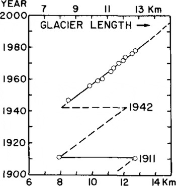
The velocity profile along the centre line of the tongue deduced from the more recent measurements can be fitted by a smooth curve (Fig.3). This implies that there are no significant local accelerations and decelerations along the centre line. The possibility of local velocity fluctuations cannot be ruled out but they seem unlikely. It has thus been assumed that EGT is free-floating beyond the hinge line.

Fig.3 Ice flow rates, determined from Figure 2 and from direct measurement. Horizontal strain-rates as well as a direct measurement (solid circle) are also given. The time scale is derived from these data.
It will be noted that the glacier is curved in plan, concave to the north. Thus, extensive strainrates along the southern edge should exceed those along the northern edge, if it were demonstrated that part or all of the bending was due to current pressure exerted against the side of the glacier. In this case, the flow rates along the south edge would exceed those along the centre line and along the north edge. Since previous flow rates were derived from the set of southerly teeth, the effect of a “curvature” correction to the strain-rate data of Figure 6 in Reference HoldsworthHoldsworth (1974) would tend to shift the line to the right, closer to the line taken fromReference Thomas Thomas (1971). In addition, a slight, but systematic, numerical error in the computation of the “effective” stress τ inReference Holdsworth Holdsworth (1974) led to the line being too far to the left of theReference Thomas Thomas (1971) line. In this paper, we compute τ using the average column density ρ to avoid the numerical integration otherwise necessary.
A prediction for the probable timing of the next calving event was given in Reference HoldsworthHoldsworth (1974). The identified interval (1972-77) was based on one previously observed calving (1911), photographically derived growth rates of the glacier, and on the implicit assumption that open ocean conditions would prevail at the time high-energy wave motion was transmitted into EGT. On the basis of new information, figure 3 inReference Holdsworth Holdsworth (1974) can now be updated and an explanation for the apparent delay in calving will be given. Part of this explanation rests on the observation that in recent years the sea ice has remained around the glacier in situ, except in the immediate area of the terminus. Not only has the sea ice the effect of damping-out ocean-wave swell amplitudes (and hence reducing bending stresses in the glacier), but also, from energy considerations, it appears that it may exert significant resistance to the deformation of EGT in its lateral bending and, probably, to its seaward expansion. This latter effect becomes more important as the thickness of EGT diminishes by creep thinning and by melting.
There are two imminent possibilities for the calving of EGT: (a) by oscillation in one of the natural modes (resonant motion) (Reference Holdsworth and GlynnHoldsworth and Glynn 1981), and (b) by hinge-line bending under current pressure, where the bending stress follows an accelerated increase as the fracture is driven progressively across the width of EGT.
1. Physical measurements up to 1978.
1.1. Mapping
Remapping of EGT from 1947 to 1978 was carried out using a variety of methods of differing reliability: 1947, 1956, 1959, 1960, 1962, and 1965 US Navy aerial oblique photographs were used to plot maps using a Wilson photoalidade.
In 1966 and 1967, US Navy vertical photographs cover only parts of EGT, whereas in 1970 and 1978 complete coverage by vertical photography was obtained on request. The January 1970 map was plotted stereophoto grammetrically, without ground control, and the original map was ˜9% too large, since the uncorrected aircraft altimeter reading was used. Controlled (January 1978) photos were not acceptable for stereo-plotting so the map was constructed by the radial line method. The assumption was made that between 1970 and 1978, approximate steady-state thickness conditions prevailed (section 1.6). A reduction transform was then applied to the surface elevations on the 1970 map; the same transform was applied in the horizontal plane. Less reliable maps were produced for 1947, 1956, 1959, 1960, 1965, and 1967. Outlines for 1972, 1974, and 1976 were obtained from LANDSAT imagery.
1.2. Ice-flow rates from marginal tooth displacements
Individual teeth were numbered (14 on each edge). Each tooth was identified on preceding maps, where possible, and its distance from the hinge-line origin measured. Despite massive melt-back and calving, it was found possible to place some reliability on the time-distance plots (Fig.2).
1.3. Direct measurement of ice displacement
From 26 December 1977 to 25 January 1978, the positions of 12 reference poles were determined by resection to seven control points (Fig.l[c]).Elevation differences were corrected for curvature and refraction as well as for tidal variation. Most poles were surveyed three times. Due to scatter in the data, it is not possible to resolve the transverse velocity gradient. The data (Fig.3) are therefore taken to apply along the centre line, and the smooth curve put through the points is used to derive the longitudinal strain-rate. Velocities derived from tooth displacements are plotted in Figure 3; a possible higher average velocity seems to occur on the southern margin, particularly towards the hinge. The reliability of the derived strain-rates is shown by plotting a measurement made using a wire strainmeter (Reference Goodman and HoldsworthGoodman and Holdsworth 1978).
1.4. Ice thickness and water depths
Airborne radar has been flown along the centre line of EGT in 1967, 1978, and 1979 by the combined NSF/SPRI/TUD operation. For ice thinner than about 140 m, interpretation of ice bottom returns is complicated by possible returns from the marginal indentations and surface crevasses. Figure 4 shows the adopted geometric centre-line ice thickness. Absolute and relative errors in thickness are √15 m and ±10 m, respectively. Thickness at the margins is roughly 0.75H, where H is the centre thickness. Water depths were measured at 15 edge sites by calibrated tag-line. About 250 to 500 m of the northern edge seems to be resting on the ocean bottom, but there is no evidence of further grounding.

Fig.4. Data for EGT: ice thickness along the centre line with computed temperatures, sea-water temperatures, surface and basal ice balances
1.5. Surface net mass balance, density, and temperature
The surface net balance was estimated from measurements made at an array of wooden posts installed in 1973 by New Zealand Ministry of Works personnel. From measurements made up to 1977-78 an approximate balance curve has been derived (Fig.4). Firn densities were measured on core samples taken to 10.5 m depth, and these varied from 0.45 to 0.65 Mg m−3. The 10 m temperature was -19.8±0.1°C.
Basal ice temperatures derived from equivalent water-depth temperatures (Reference Jacobs, Huppert , Holdsworth and DrewryJacobs and others 1981) are given in Figure 4. From these data, a steady-state finite element simulation of EGT temperature has been performed, in order to determine the mean column temperature along the centre line of EGT. Mean temperatures range from -14 to -12°C (see section 2).
1.6. Mass balance of EGT
The mass-balance equation (Reference BuddBudd 1966) is:
where ![]() is the surface net balance
is the surface net balance ![]() is the basal balance
is the basal balance  is the average glacier column density,ρi is the density of ice,
 ![]() is the vertical strain-rate, Vx is the horizontal velocity component, and H is the total ice thickness at distance x from the hinge line. For steady state ∂H/∂t = 0 and (1) may be solved for
is the vertical strain-rate, Vx is the horizontal velocity component, and H is the total ice thickness at distance x from the hinge line. For steady state ∂H/∂t = 0 and (1) may be solved for ![]() .
.
Values of ![]() thus derived are shown in Figure 4. Despite large errors in H and ∂H/∂t, there appears to be a trend of increasing melt rate toward the free end except at x=10 to 11 km where some freezing may occur. That melting is taking place is positively indicated by the results of Reference Jacobs, Huppert , Holdsworth and Drewry Jacobs and others (1981), which show steps in conductivity-temperature-depth (CTD) profiles taken to depths of 250 m close to EGT.
thus derived are shown in Figure 4. Despite large errors in H and ∂H/∂t, there appears to be a trend of increasing melt rate toward the free end except at x=10 to 11 km where some freezing may occur. That melting is taking place is positively indicated by the results of Reference Jacobs, Huppert , Holdsworth and Drewry Jacobs and others (1981), which show steps in conductivity-temperature-depth (CTD) profiles taken to depths of 250 m close to EGT.
2. Re-analysis of flow law for egt ice
2.1. Derivation of flow law “viscosity” parameter B
The flow law is assumed to be of the form:
where
is the effective strain-rate, and
is the effective stress, ![]() is the component of strain-rate and
is the component of strain-rate and ![]() is the component of the deviator stress in which (i,j)=(x,y,z) (x-longitudinal, y-transverse and z-vertical). B is dependent on ice temperature, structure, and impurity; n is usually, and will herein be taken as, 3.
is the component of the deviator stress in which (i,j)=(x,y,z) (x-longitudinal, y-transverse and z-vertical). B is dependent on ice temperature, structure, and impurity; n is usually, and will herein be taken as, 3.
It may be shown that vertical plane shear stresses are small compared to normal stresses. The maximum value of σzx is (Reference Sanderson and DoakeSanderson and Doake 1979):
where h = (l–ρ/ρw)H in which ρw is the density of seawater. Substituting h=32 m, H=208 m, dh/dx=0.0025, (x=4000 m),
Other stresses of the type σij(i≠j) are assumed to be small, except possibly at the hinge line or in the region of re-entrants
Values of ![]() and τ were computed using Equations (2a) and (2b) (Reference ThomasThomas 1973). In (2a) the vertical strain-rate
and τ were computed using Equations (2a) and (2b) (Reference ThomasThomas 1973). In (2a) the vertical strain-rate ![]() was determined from the (approximate) incompressibility relationship to be
was determined from the (approximate) incompressibility relationship to be
where ![]() is taken as ˜0.9 rather than 1.0 (section 3).
is taken as ˜0.9 rather than 1.0 (section 3).
The plot of ![]() points is shown in Figure 5. Individual values of B may be computed from these data using Equation (2) and assuming n=3. The results are shown in the following tabulation:
points is shown in Figure 5. Individual values of B may be computed from these data using Equation (2) and assuming n=3. The results are shown in the following tabulation:


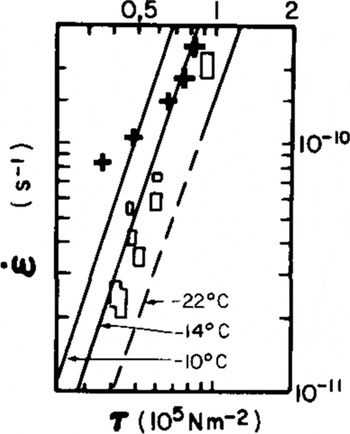
Fig.5 Plot of effective strain-rate ![]() vs effective stress (τ) for points on centre line of EGT. Line slopes are for n = 3 for temperatures given inReference Thomas Thomas (1973[b]). (Open rectangles are data from other ice shelves.)
vs effective stress (τ) for points on centre line of EGT. Line slopes are for n = 3 for temperatures given inReference Thomas Thomas (1973[b]). (Open rectangles are data from other ice shelves.)
These data may be interpreted as follows: as the ice thins and the mean ice temperature increases, and as crevasse depths are a significant fraction of the total ice thickness, the ice tends to become "softer" This would evidently explain the apparent drift of points away from a straight line in Figure 5. Thus the strain-rates are higher than expected for a given effective stress.
There is now better agreement with the data of Reference ThomasThomas (1973). The “equilibrium” profile study of EGT (Reference SandersonSanderson 1979) should now be revised with B= B(x). The now greater effective viscosity of the ice near the hinge line would result in slower thinning rates there, and render, as required, a better model fit to the data in the hinge zone (Reference SandersonSanderson 1979: 441).
3. Curvature of egt
3.1. Geometry
From Figure 1 it may be seen that a transverse asymmetry develops with time; the thickest ice becomes closer to the south edge, as a result of progressive melting along the southern edge, which greatly exceeds melting along the northern edge. A dynamic centre line is shown on the 1970 map. Figure 6 shows a plot of the radius of curvature of this line. Despite the large scatter in data points, an increase in curvature with distance (x) is quite apparent. A possible initial curvature may be due to differential exit speeds on either side of the hinge line.

Fig.6 Curvature of dynamic centre line of EGT, measured from Figure 1. Points obtained by two operators from 1970 and 1978 maps.
3.2. Lateral half-widths of EGT and determination of melt rates
Figure 7 shows the half-widths for the northern and southern sides of the dynamic centre line : melting is clearly most severe on the southern side to the extent that lateral creep spreading is completely obliterated. On the northern side, lateral spreading is seen as far as x≈5 km, before melting-back dominates. In order to compute melt rates, it is necessary to compute the lateral spreading due to Weertman creep (Reference WeertmanWeertman 1957). Plots Of half-widths for different ![]() are shown in Figure 7, and a value of α= 0.9 is considered likely. A time scale (Fig.3) was established using
are shown in Figure 7, and a value of α= 0.9 is considered likely. A time scale (Fig.3) was established using

From this, the incremental spreading ∆y is computed for distance steps ∆x of 500 m (∆t ˜ 4a): ![]() The resulting theoretical half-wraths minus the measured half-widths give the meltback (Fig.7). These melt rates probably correspond with the average surface water temperature of -1.3°C (Reference Jacobs, Huppert , Holdsworth and DrewryJacobs and others 1981) and are shown in Figure 8 together with basal melt rates which fall below the line of Reference Morgan, Budd and HusseinyMorgan and Budd (1978), possibly because of lower water speeds on the bottom surface. Differential melt rates on either side of EGT thus increase its apparent curvature over the curvature due to creep bending.
The resulting theoretical half-wraths minus the measured half-widths give the meltback (Fig.7). These melt rates probably correspond with the average surface water temperature of -1.3°C (Reference Jacobs, Huppert , Holdsworth and DrewryJacobs and others 1981) and are shown in Figure 8 together with basal melt rates which fall below the line of Reference Morgan, Budd and HusseinyMorgan and Budd (1978), possibly because of lower water speeds on the bottom surface. Differential melt rates on either side of EGT thus increase its apparent curvature over the curvature due to creep bending.

Fig.7 Plot of half-widths of EGT measured from the dynamic centreline. Spreading rates for the transverse strain factor α = 0.5, 0.9, and 1.0 are shown. Derived melt rates for the north and south edges are given

Fig.8 Ice melt rates versus water temperature
3.3. Curvature induced by dynamic processes
The curvature of the “dynamic” centre line may be caused by differential exit speeds on either side of the hinge line or by ocean current pressure exerted from the south
3.3.1. Differential exit speeds
Figure 3 shows that if there is a difference in flow rates on either side of the hinge line, it is not greater than about the error of the measurements (±5 m a−1). If Vn and Vs are the exit speeds on the north and south edges, separated by a full glacier width of W0, then the curvature generated at the hinge line would be
and for Vs -Vn = 1 m a−1, (Vn +Vs)/2 = 85 m a−1, and W0 ˜ 2 000 m,
An initial curvature of this magnitude may be possible (see Fig.6).
3.3.2. Current pressure acting on the south edge of EGT
Because melt rates on the southern edge have been shown to be about three times those on the northern edge (Fig.7) and because curvature increases with distance from the hinge line (Fig.6), the effects of ocean current pressure on EGT must be examined. As no direct current measurements are available in the vicinity of EGT, we use the following information: (i) visual evidence for a northward current sweeping around EGT can be seen in figure 1 of Reference HoldsworthHoldsworth (1974) (see also Reference Holdsworth and GlynnHoldsworth and Glynn 1981), (ii) holes drilled through the sea ice on the south side produced turbulent up wellings (holes on the north side apparently did not), and (iii) hydrographic and sailing manuals for Antarctica indicate the existence of a strong (3 knots (1.5 m s−1)) current setting north around the coast in the vicinity of EGT
A water current of uniform speed is assumed to flow into EGT from the south and to lose momentum to the glacier. A mean current flow constant with depth and distance from the coast is taken as 1 knot (0.5 m s−1). We wish to determine the bending moment and, subsequently, the bending stresses induced in EGT. For these purposes, the form of EGT is somewhat idealized to facilitate computation. If the force acting on an elemental area of EGT of length dx and height ![]() is 0.5 CD ρ H Vc
2 dx, where CD is the form drag coefficient (˜1.95) and Vc is the current speed (H is taken as in ((1)),then the moment Mx
'of this force about a vertical axis at x' from the origin is
is 0.5 CD ρ H Vc
2 dx, where CD is the form drag coefficient (˜1.95) and Vc is the current speed (H is taken as in ((1)),then the moment Mx
'of this force about a vertical axis at x' from the origin is

(see Reference Holdsworth and GlynnHoldsworth and Glynn (1981)). The resulting moment distribution is shown in Figure 9. The maximum (edge) bending stress at x' is
where W is the actual width as measured from Figure 1, and n = 3 (section 2). H e is the “effective thickness” of EGT (0.75H< He < H). (The effective thickness is H minus crevasse depth, ~30 m.) Figure 9 shows values of ![]() (max). The highest stresses can occur beyond the hinge line, depending on the variation of W(x) and, to a lesser extent, on the local variations of He. Thus, some significant stress maxima may occur far from the hinge line. The bending stress and creep strain history of selected points along the edge of EGT will now be examined to see if curvatures comparable to the observed curvatures (Fig.6) may be generated. It is necessary, first, to present the history of the length variations of EGT (Fig.10). Figure 11 presents the time variation of bending stress for three selected points on the edge of EGT using the information in Figure 10, Equations (5) and (6) and a deduced value of dW/dt.
(max). The highest stresses can occur beyond the hinge line, depending on the variation of W(x) and, to a lesser extent, on the local variations of He. Thus, some significant stress maxima may occur far from the hinge line. The bending stress and creep strain history of selected points along the edge of EGT will now be examined to see if curvatures comparable to the observed curvatures (Fig.6) may be generated. It is necessary, first, to present the history of the length variations of EGT (Fig.10). Figure 11 presents the time variation of bending stress for three selected points on the edge of EGT using the information in Figure 10, Equations (5) and (6) and a deduced value of dW/dt.

Fig.9 Plot of bending moment and bending stress EGT (1978

Fig.10 Length-time record for EGT (1902 to present)
Next, the strain-rates corresponding to these stresses will be computed. The assumption is made that bending and linear creep stresses may be directly superimposed. At a particular point on the edge of a smooth margined EGT model, the stress (deviator) components become
where ![]() is the bending stress in the edge parellel to the x-axis and
is the bending stress in the edge parellel to the x-axis and ![]() is the Weertman creep stress in the same direction. The transverse component of the creep stress
is the Weertman creep stress in the same direction. The transverse component of the creep stress ![]() is assumed to be 0.9
is assumed to be 0.9 ![]() A flow law of the same form as Equation (2) is assumed, so that in component form
A flow law of the same form as Equation (2) is assumed, so that in component form
where B and n are the values obtained previously
The creep rates ![]() are computed separately using Equation (7) to obtain
are computed separately using Equation (7) to obtain ![]()
The stresses shown in Figure 11 were used to compute, in stages, the value of ![]() for each stress level, and the total creep bending increment ∆lover length l was then computed from
for each stress level, and the total creep bending increment ∆lover length l was then computed from ![]() where ∆t and ∆x,are the time and distance increments, respectively
where ∆t and ∆x,are the time and distance increments, respectively

Fig.11 Bending stress history for selected points (Fig.1(b)) on north and south edges of EGT, with and without Weertman creep
The mean curvature R –1 over l is obtained from the expressions
For point A (Fig1(b)) travelling a total distance l˜9 500 m, the mean curvatur ![]() , which is greater than the mean observed curvature (Fig.6) by a factor of 6. This discrepancy may be explained by any or all of the following: (i) the value of B used in Equation 7 is too low, (ii) the water current speed (and hence pressure) assumed to be incident on EGT is too high, and (iii) the presence of fast ice around EGT retards lateral deformation.
, which is greater than the mean observed curvature (Fig.6) by a factor of 6. This discrepancy may be explained by any or all of the following: (i) the value of B used in Equation 7 is too low, (ii) the water current speed (and hence pressure) assumed to be incident on EGT is too high, and (iii) the presence of fast ice around EGT retards lateral deformation.
Possible errors in B and Vc are unlikely to account for the above discrepancy, except possibly if cases (i) and (ii) occur together. More likely, however, is case (iii): consider the compressive stress induced in the sea ice as a result of the pressure exerted on EGT. A normal stress of magnitude
would be induced in the sea ice of thickness hj. For typical values of H = 200 m, and Hj = 3.5 m, this stress is ~0.013 MN m−2 which is probably sufficient to cause only very slow creep in the sea ice. If we next assume that lateral deformation is essentially only allowed over 1/6 of the total time (or an average of two months per year), then the curvature, recomputed through Equation 8, becomes about 40 × 10−6 m−1. This is now approximately equal to the observed curvature. The complete history of breakout of fast ice around EGT is not known. It is, however, known that breakout does not occur every year, although the ice probably becomes loose and weak around the glacier. Such a condition might allow significant deformation of EGT during the summer
Another possibility, not considered above because of lack of information, is that a northward current does not prevail throughout the entire year.
4. Short-period oscillations of egt
The theory of wave-induced oscillations for a simplified EGT model is given in Reference Holdsworth and GlynnHoldsworth and Glynn (1981) and measurements of tilt and strain-rate confirming these oscillations were reported in Reference Goodman and HoldsworthGoodman and Holdsworth (1978) and Reference Holdsworth and HoldsworthHoldsworth and Holdsworth (1978). Details will be reported elsewhere.
Such oscillations, considered important in calving theory, may also be significant in terms of the apparent softening of EGT ice thinner than ˜150 m. Only some of this softening may be explained by the bulk warming of the glacier (Fig.4).
Surface crevasses exist in profusion. For a crevasse depth of 30 m (0.2 to 0.4H) the effective thickness of EGT is greatly reduced, and time varying stress concentrations would exist at crevasse tips, enhancing horizontal creep. If basal freezing occurs, basal crevasses would be unlikely (Reference WeertmanWeertman 1980) despite warmer ice, the existence of a water current, and the oscillations.
5. Calving of egt
5.1. Vibration calving mechanism
Calving of EGT was dfscussed in Reference Holdsworth and GlynnHoldsworth and Glynn (1981) with particular emphasis on the vibration mechanism acting as a trigger. Evidently, open water conditions are necessary for this mechanism to be sufficiently activated. Local bending stress maxima may occur far from the hinge line (Reference Holdsworth and GlynnHoldsworth and Glynn 1981 and Fig.9). A particularly vulnerable section is indicated by B in Figure 1(b). This is approximately the line of the 1911 calving (and presumably, also, the 1942 calving). The localized vertical thinning between 8 and 9 km (Fig.4) is associated with a pronounced surface valley and is a potential location for calving in the future.
5.2. Calving at the hinge line by horizontal bending
It is of interest to examine the history of the bending stress at the hinge line, particularly since the three most easterly teeth on the south edge have recently disintegrated (Fig.1(b)). The 1978 width of EGT at the section G-H was 860 m, whereas in 1970 the narrowest section was 1300 m; and all previous maps show, in general, at least a 1000 m width, given the uncertainties in mapping accuracy.
The south edge hinge-line tensile stress has been computed using Equations (5) and (6) and results are shown in Figure 12, where the time scale is keyed to that in Figure 10. It may be seen that the rate of increase of tensile stress due to bending is decreasing with time because the thinning, advancing ice exerts a progressively smaller bending moment at the hinge. If basal melting predominates, the hinge-line width remains constant at 1200 m and no calving occurs (an unlikely situation); then the maximum length of EGT, of about 16 km, would be reached shortly after 2000 AD.
From recent field observations (R Holdsworth private communication), it appears that the re-entrant rift at the hinge line is becoming deeper, hence by Equation (6), since W is decreasing, ![]() must be increasing (beyond the values given in Figure 12 which has been computed using a typical average glacier width W = 1200 m). A potential feedback stress-width regime now exists, since
must be increasing (beyond the values given in Figure 12 which has been computed using a typical average glacier width W = 1200 m). A potential feedback stress-width regime now exists, since ![]() and the stress (or the accompanying strain-rate) will tend to drive a re-entrant or crack deeper into the glacier, reducing W.
and the stress (or the accompanying strain-rate) will tend to drive a re-entrant or crack deeper into the glacier, reducing W.

Fig.12 Idealized south edge hinge tensile stress vs time for constant width w = 1200 m) and thickness H. Maximum and minimum stresses derived using an effective thickness of 0.75H and H (H = 340m). Steep lines beginning 1976-78 indicate actual recent stress development.
6. Conclusion
The geometry and flow of EGT is evidently influenced both by the sea-water in which it floats and by the sea ice surrounding it. The former is exerting a destructive influence, while the latter is performing a protective role
Although some local basal freezing may occur, basal ice melting predominates and is more responsible than creep thinning for the thickness profile of EGT. Marginal ice melt is taking place on the south edge up to three times faster than on the north edge due, evidently, to a sea-water current flowing into EGT from the south. It is shown that this current may be largely responsible for the pronounced curvature of EGT, and that the bending stresses induced in the glacier may lead to its destruction before other potential calving mechanisms are activated.
It would appear that the presence of fast ice tends to reduce the amount of lateral bending in EGT. Moreover, the glacier becomes coupled to the sea ice in the longitudinal direction by the tooth and reentrant structure which extends the full length of EGT. Shear cracks in the sea ice (Fig.1(b)) indicate the extent of this coupling
The outer, thinner parts of EGT are evidently weakened by the high density of crevasses; this, together with the fact that the thinner ice is warmer than the coastward ice, renders it “softer” than the latter
Oscillations occurring in EGT are in response to wave swell forcing and many peak frequencies coincide with or are close to the computed natural frequencies of EGT. The potential exists for a calving induced by forced vibration of EGT in one of its higher modes (Reference Holdsworth and HoldsworthHoldsworth and Holdsworth 1978), but such an event may be pre-empted by horizontal bending failure at or near the hinge line.
Acknowledgements
I thank the US National Science Foundation (Division of Polar Programs) for support enabling essential field work to be carried out. The US Navy supplied photography from which the maps were prepared, and hydrographic data. In the field, I was helped extensively by D J Goodman and R Holdsworth. Discussions with them, R F Henry, G de Q Robin, and C Holdsworth on various aspects of the work are much appreciated. F Mirza and D Stolle did the numerical temperature computations (Fig.4), T J Chinn supplied some pole measurements and D J Drewry, D Mel drum, E Jankowski, and H Steed provided the ice-thickness data. J Clarkson assisted with the mapping and curvature measurements. S S Jacobs provided oceanographic data. M Metge and F Mirza checked parts of the manuscript.