


Introduction
The vast majority of Earth's freshwater is stored in the Antarctic ice sheet and because of this large volume (>55 m sea-level equivalent (SLE); Nowicki and others, Reference Nowicki2013; Albrecht and others, Reference Albrecht, Winkelmann and Levermann2020; Morlighem and others, Reference Morlighem, Rignot, Binder, Blankenship and Drews2020), the loss of even a small fraction of its mass could soon dominate sea-level rise. Reconstructions of past sea level show that the ice sheet could have contributed between 10 and 20 m SLE during the Pliocene, a period stretching between 5.3 and 2.6 million years before present with global mean temperature $2\hbox {--}3^\circ {\rm C}$ higher than present-day (Miller and others, Reference Miller2012; Grant and others, Reference Grant2019). Current observed mass loss from the Antarctic ice sheet is accelerating and concentrated in the Amundsen Sea area (Mouginot and others, Reference Mouginot, Rignot and Scheuchl2014; Rignot and others, Reference Rignot, Mouginot, Morlighem, Seroussi and Scheuchl2014; Shepherd and others, Reference Shepherd2018) and the Aurora Subglacial Basin, including Totten Glacier (Khazendar and others, Reference Khazendar2013). These changes have been attributed to variations in ocean circulation bringing warm, intermediate-depth waters into contact with the base of ice shelves (Payne and others, Reference Payne, Vieli, Shepherd, Wingham and Rignot2004; Thomas and others, Reference Thomas2004; Jenkins and others, Reference Jenkins2010; Pritchard and others, Reference Pritchard2012; Paolo and others, Reference Paolo, Fricker and Padman2015; Jenkins and others, Reference Jenkins2018).
Despite recent advances in modelling marine ice sheets (Pattyn, Reference Pattyn2018), projections of the future contribution of the Antarctic ice sheet to sea level are still hampered by insufficient knowledge of atmospheric and oceanic forcings and the impact of those forcings on critical ice-sheet model physics and dynamics (Pattyn and others, Reference Pattyn2018). This is exemplified by the hypothesis of new physical mechanisms, such as the Marine Ice Cliff Instability (MICI; Bassis and Walker, Reference Bassis and Walker2012; Pollard and others, Reference Pollard, DeConto and Alley2015), which leads to significantly larger sea-level contributions for the Antarctic ice sheet compared to other studies (DeConto and Pollard, Reference DeConto and Pollard2016). However, additional studies conclude that major ice loss during the Pliocene Epoch could also be reached without such mechanisms (Bulthuis and others, Reference Bulthuis, Arnst, Sun and Pattyn2019; Edwards and others, Reference Edwards2019; Golledge and others, Reference Golledge2019). Other uncertainties stem from the timing and processes that govern ice-shelf weakening, disintegration and collapse (Pattyn and others, Reference Pattyn2018).
Thinning of ice shelves, and concomitant reduction in ice-shelf buttressing, leads to grounding line retreat, inland ice acceleration and loss of grounded ice mass (Pritchard and others, Reference Pritchard2012). Reduction in ice-shelf buttressing has an almost instantaneous effect on ice flow, which implies that this process can result in rapid changes in ice flux over the grounding line (Reese and others, Reference Reese, Gudmundsson, Levermann and Winkelmann2018b; Gudmundsson and others, Reference Gudmundsson, Paolo, Adusumilli and Fricker2019). Ice-shelf thinning and weakening due to specific interactions with atmosphere (surface melt, meltwater percolation, refreezing and runoff; Trusel and others, Reference Trusel2015) and ocean (changes in ocean circulation, ocean warming and sub-ice-shelf melting; Alley and others, Reference Alley2015; Thompson and others, Reference Thompson, Stewart, Spence and Heywood2018) are parameterized with a large variation in ice-sheet models (Favier and others, Reference Favier2019).
In this paper, we investigate how changing ice shelves control Antarctic mass loss independent of the triggers for how and when ice shelves weaken. Previous ice-sheet intercomparison efforts (Pattyn and others, Reference Pattyn2012, Reference Pattyn2013; Bindschadler and others, Reference Bindschadler2013; Nowicki and others, Reference Nowicki2013; Seroussi and others, Reference Seroussi2019) highlighted the importance of better assessing the causes of the variation in model results, and separating differences associated with model grid resolution, ice dynamics (e.g. choice of stress balance equation), physical processes included (e.g. calving, hydrofracture and cliff failure), initialization procedure (e.g. data assimilation, spin-up or relaxation) and numerical schemes. We designed a simple experiment that considers an instantaneous and sustained removal of floating ice. This scenario is not realistic, but allows us to investigate how different ice-sheet models cope with the impact of a sudden, complete loss of ice-shelf buttressing. By removing the uncertain causes related to ice-shelf thinning and weakening, we are able to isolate uncertainties in the response of the grounded ice sheet to grounding-line retreat due to loss of ice-shelf buttressing. We analyse 15 simulations from 13 international groups in order to determine the most relevant factors controlling the rate of Antarctic mass changes in an extreme mass loss scenario. Furthermore, the absence of buttressing may lead to ice-sheet collapse through the marine ice-sheet instability (MISI) in areas where the bed deepens towards the interior of the ice sheet. The experiment therefore enables to quantify the MISI potential and associated uncertainties for the Antarctic ice sheet and revises estimates of this potential that have previously been made for the West Antarctic ice sheet (Bamber and others, Reference Bamber, Riva, Vermeersen and LeBrocq2009).
This experiment is coordinated through the Antarctic BUttressing Model Intercomparison Project, ABUMIP (http://www.climate-cryosphere.org/wiki/index.php?title=ABUMIP-Antarctica), endorsed by the Ice Sheet Model Intercomparison Project, ISMIP6 (http://www.climate-cryosphere.org/activities/targeted/ismip6), part of the Coupled Model Intercomparison project, CMIP6 (https://www.wcrp-climate.org/wgcm-cmip/wgcm-cmip6). It builds on the ISMIP6 initialization experiments (http://www.climate-cryosphere.org/wiki/index.php?title=InitMIP-Antarctica) for the Antarctic ice sheet (Seroussi and others, Reference Seroussi2019), in which most of the models in this study participated (see Appendix for details on each model). The main purpose of ABUMIP is to gauge the sensitivity of different ice-sheet models with respect to such grounding-line retreat, whether they pertain to numerical methods, physical approximations or boundary conditions. It also enables evaluation of the sensitivity of models that are used for the full Antarctic, for global sea-level rise projections (Seroussi and others, Reference Seroussi2019). While similar experiments have been done previously by Cornford and others (Reference Cornford, Martin, Lee, Payne and Ng2016), Golledge and others (Reference Golledge, Levy, McKay and Naish2017, supplementary material) and Pattyn (Reference Pattyn2017), we are able to put these results into a wider context through a controlled experiment and by examining a large number of diverse models. This will help to better understand the spread in projections of 21st century Antarctic ice sheet contributions to sea level.
Experiments and model setup
Description of the experiments
ABUMIP consisted of three experiments, a control run (ABUC) and two forcing experiments (ABUK and ABUM) that controlled the rate of loss of ice shelves. All experiments started from an initialized present-day state of the Antarctic ice sheet, as defined by the initMIP-Antarctica (Seroussi and others, Reference Seroussi2019). All ABUMIP experiments ran for a period of 500 years forward in time.
Control run (ABUC)
Similar to Seroussi and others (Reference Seroussi2019), atmospheric and oceanic forcings in the control run were assumed to be similar to present-day conditions, without any extra forcing aside from that applied at the end of the initialization.
Ice-shelf removal or ‘float-kill’ (ABUK)
For the first forcing experiment, all floating ice (ice shelves) surrounding the ice sheet was removed at the start of the run and thereafter any newly-formed floating ice was instantaneously removed (so-called ‘float-kill’). In other words, at all times, calving flux was assumed to be larger than the flux across the grounding line to prohibit regrowth of the shelves.
Extreme sub-ice-shelf melt (ABUM)
The second experiment applied an extremely high constant melt rate of 400 m a−1 underneath the ice shelves. Similar experiments have been carried out in previous studies with basal melt rates ranging from 200 m a−1 in Bindschadler and others (Reference Bindschadler2013) to 400 m a−1 in Cornford and others (Reference Cornford, Martin, Lee, Payne and Ng2016). Such high forcings inevitably lead to rapid loss of ice shelves and hence of buttressing. Preliminary experiments have shown that the actual value within the range found in the literature is of lesser importance.
Model setup
Participating ice-sheet models were free to choose the initialization procedure, which is generally dependent on the given model characteristics and requirements. There were no further constraints on present-day forcing datasets applied (including surface mass balance, surface temperature and sub-shelf melt rates) or on specific physical processes and parameterizations included in the models (e.g. basal sliding and friction laws, ice rheology and stress balance approximation). Isostatic adjustment was not considered. The initialization time varies among models but was near the beginning of the 21st century.
Models were required to represent ice shelves and grounding line dynamics, and the initialization process should include ice shelves. Ice-sheet models applied the present-day surface mass balance (SMB) and basal mass balance (BMB) of their choice, but without adjusting for the impacts of geometric changes in the forward experiments (i.e. no SMB, surface-elevation feedback). Finally, models used the bed and surface topography of their choice, while bedrock elevation adjustment and processes affecting ice shelves (other than sub-shelf melting) were not taken into account. Model output was taken in the same format as for the initMIP-Antarctica experiments (Seroussi and others, Reference Seroussi2019) but for 500 years instead of 100 years after being initialized to the beginning of the 21st century.
Participating models
A total of 13 modelling groups participated in the experiments and most of these performed all the three experiments (Table 1). Details of the 15 different models, their initialization, their numerical characteristics and which sliding or friction laws are employed are summarized in Table 2. Time steps from 0.4 days to 0.5 years are used by models. Further description of the models can be found in the Appendix.
Table 1. List of participating models in the ABUMIP experiment
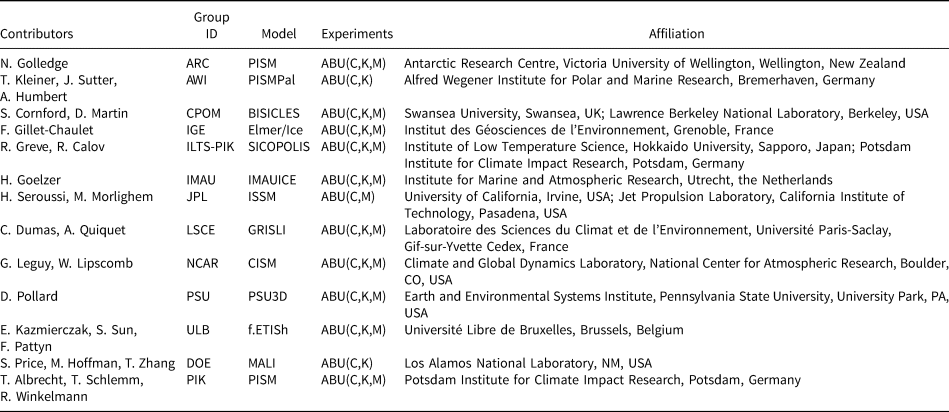
Details of the models are given in Table I and Appendix.
Table 2. List of ABUMIP simulations and main model characteristics

Numerics rely on the finite-difference (FD), finite-element (FE) or finite-volume (FV) method. Stress balance approximations implemented by models include Shallow-Shelf Approximation (SSA; see MacAyeal, Reference MacAyeal1989), SSA with vertical shear terms represented in the effective viscosity term (SSA*; see Cornford and others, Reference Cornford2013), combination of SSA and Shallow-Ice Approximation (Hybrid; see Bueler and Brown, Reference Bueler and Brown2009; Winkelmann and others, Reference Winkelmann2011), depth-integrated higher-order approximation (L1L2; see Goldberg, Reference Goldberg2011) and Blatter–Pattyn approximation (LMLa; see Pattyn, Reference Pattyn2003). Initialization methods are as follows: spin-up (Sp), spin-up with target values for the ice thickness (SpC), data assimilation (DA), equilibrium state (Eq) and equilibrium state with target values for the ice thickness (EqC; see Pollard and DeConto, Reference Pollard and DeConto2012a). (+) Means relaxation after initialization. ($\star$ ) Marks models that use a grounding line flux parameterization (e.g. Pollard and DeConto, Reference Pollard and DeConto2012a). Initial SMB is derived from the following: RACMO2 (Lenaerts and others, Reference Lenaerts, van den Broeke, van de Berg, van Meijgaard and Kuipers Munneke2012), RACMO2.3 (Van Wessem and others, Reference Van Wessem2014), RACMO2.3p2 (Van Wessem and others, Reference Van Wessem2018), MAR (Agosta and others, Reference Agosta, Amory, Kittel, Orsi and Favier2019) and Arthern and others (Reference Arthern, Winebrenner and Vaughan2006) (Arthern). Ice-sheet geometries are based on Bedmachine (Morlighem and others, Reference Morlighem, Rignot, Binder, Blankenship and Drews2020) for f.ETISh and Bedmap2 (Fretwell and others, Reference Fretwell2013) for all other models. Further details on all the models are given in the Appendix.
All models include membrane stresses in their force balance, either corresponding to the so-called Shallow-Shelf Approximation (SSA, Table 2), or by also including vertical shearing and vertically differentiated membrane stresses. The majority of models are hybrid models and heuristically combine the SSA as a sliding or friction law with the Shallow-Ice Approximation (SIA) for inclusion of vertical shearing (Bueler and Brown, Reference Bueler and Brown2009). One model includes vertical shear terms in the effective viscosity term (Schoof and Hindmarsh, Reference Schoof and Hindmarsh2010), which leads to the so-called SSA* approach. One model applies the Blatter–Pattyn approximation (labelled LMLa), which is the hydrostatic approximation of the Stokes equations (Blatter, Reference Blatter1995; Pattyn, Reference Pattyn2003), and one model (labelled L1L2) uses a depth-integrated version of this approximation (Goldberg, Reference Goldberg2011).
The participating models use several different initialization techniques. A common approach is the paleo spin-up (Sp, Table 2) during which the ice sheet is run through a glacial-interglacial cycle until the present day. In this way, the state includes temperature field and change rates of geometry as cumulative response to past climates. In one case, the spin-up runs with an iterative optimization for basal friction coefficients with target values for ice thickness (SpC). Another common procedure is an equilibrium type spin-up, which also allows for establishing an internal temperature field with equilibrium ice sheet (Eq). In most cases, this equilibrium ice sheet is combined with an iterative optimization of the basal sliding/friction field to obtain an ice-sheet geometry that is close to the observed ice sheet (EqC), with methods described in Pollard and DeConto (Reference Pollard and DeConto2012b) and Le clec'h and others (Reference Le clec'h2019), among others. All other models used data assimilation (essentially using the observed surface velocity field) to tune a basal friction field in present day conditions (DA). While models employing paleo spin-up (Sp) or an equilibrium state (Eq) have a present-day ice-sheet geometry that is in poorer agreement with the observed ice sheet (compared to models using assimilation methods), assimilation-based initial conditions generally have noisier and more unrealistic ice thickness transients.
Apart from the wide range of initialization techniques, discussed in more detail in Goelzer and others (Reference Goelzer2018) and Seroussi and others (Reference Seroussi2019), major model differences stem primarily from the basal sliding and/or friction law employed. Two commonly used basal conditions are the Weertman sliding (Weertman, Reference Weertman1957) and the Coulomb friction law (Schoof, Reference Schoof2005) (Table 2). Both can be written in the following generic form

where τb is the basal shear stress (sum of all basal resistance), ub is the basal sliding velocity, and β 2 a friction term that in the case of a Weertman sliding law is defined by

where C is a friction coefficient that can be spatially varying for models that use a SpC, EqC or DA initialization techniques, and N represents the effective pressure at the base of the ice sheet (difference between the ice overburden pressure and subglacial water pressure). For m = 1, the friction law becomes viscous and β 2 is solely dependent on the effective pressure. However, most models set p = 0 so that N is not considered, except ILTS-PIK-SICOPOLIS that uses p = 2. In the case of a Coulomb friction law the friction term is written using the expression as in Schoof (Reference Schoof2005) or as in Aschwanden and others (Reference Aschwanden2019)

where ϕ is the till friction angle that is either considered constant or optimized in a similar fashion to the friction term C in Eqn (2). The yield stress τc is defined by the numerator in Eqn (3), 0 ≤ q ≤ 1, and u 0 represents a threshold speed for sliding (Aschwanden and others, Reference Aschwanden, Adalgeirsdóttir and Khroulev2013). The friction law, Eqn (3), includes the case q = 0, leading to the purely plastic (Coulomb) relation τb = τcu b/|ub|. In the linear case q = 1, Eqn (3) becomes β 2 = τc/u 0 (Bueler and van Pelt, Reference Bueler and van Pelt2015). Most models define the effective pressure N from till dynamics (Bueler and van Pelt, Reference Bueler and van Pelt2015; Aschwanden and others, Reference Aschwanden2019), which leads to a sharp contrast in effective pressure between saturated till and non-saturated till or hard bedrock. None of the models considered full subglacial hydrology but either define effective pressure from subglacial elevation (submarine basins with saturated till) or from locally generated subglacial melt. The last column of Table 2 lists the values of m and q for the different friction laws employed. One model uses a Weertman law limited by a Coulomb friction law (Table 2), in which the basal shear stress is set to the minimum of the two stresses (Tsai and others, Reference Tsai, Stewart and Thompson2015).
Results
ABUC
The standard experiment of the series is the control run (ABUC), where participating models run forward for 500 years starting from the initial conditions without any external forcing. This experiment allows for determining intrinsic model drift. Despite the lack of forcing, there is a large variation in ice-sheet mass changes observed (Fig. 1; expressed in terms of contribution to sea level based on the volume above flotation as defined in Eqn (1) of Bindschadler and others, Reference Bindschadler2013), depending on the initial dataset used. The method converting ice-sheet mass loss to sea-level contribution results in ~56.7 m SLE based on the Bedmap2 data set, which is lower than the value 58.3 m in Fretwell and others (Reference Fretwell2013) using the Lambert Azimuthal Equal Area projection for area and volume calculations. For BedMachine Antarctica (Morlighem and others, Reference Morlighem, Rignot, Binder, Blankenship and Drews2020) the values are ~55.1 and ~57.9 m, respectively. Results for ABUC are in overall agreement with initMIP Antarctica (Seroussi and others, Reference Seroussi2019), i.e. models that are using either data assimilation (DA) or target values for ice thickness (SpC, EqC) are closer to the present day volume of the Antarctic Ice Sheet at the start of the model run. Models that use paleo-spinup (Sp; ARC-PISM and AWI-PISMPal) overestimate the initial ice volume above flotation. One model, IMAU-ICE, underestimates the present-day ice volume, as it starts from an equilibrium ice sheet (Eq). All other models are within the range of 55–57 m SLE.

Fig. 1. Volume above flotation (in m SLE) and contribution to sea-level rise (SLR) for ABUC (left) and both ABUK and ABUM experiments (positive means higher sea-level contribution). Subplots b, c and d with title ‘-INIT’ represent the sea-level contribution compared to the initial state.
For most models, ABUC leads to a limited model drift between − 0.2 and +0.2 m SLE (Fig. 1). Exceptions are ARC-PISM with a more important mass increase equivalent to 1.5 m SLE. Models that do show a drift of around ±0.5 m SLE are PISM-PIK, DOE-MALI, PSU-PSU3D1, ULB-f.ETISh and JPL-ISSM. Model drift in the control run is generally (but not unequivocally) associated with the initialization scheme, i.e. data assimilation (DA) methods usually match better with observations but exhibit a larger drift, while the opposite is true for models relying on a spin-up or a steady-state solution (Goelzer and others, Reference Goelzer2018; Seroussi and others, Reference Seroussi2019). However, other processes could be responsible as well. For example, the suspicious mass increase in ARC-PISM could be attributed to the sub-shelf melting scheme (no melting in ABUC), and the higher mass loss (~0.5 m SLE) of PSU-PSU3D1 compared to PSU-PSU3D2 may stem from the inclusion of hydro-fracturing.
ABUK
The sudden and sustained loss of ice shelves (ABUK) or an imposed extreme high sub-shelf melt rate (ABUM) lead to a significant loss of grounded ice over the period of 500 years for all participating ice-sheet models. Net mass loss is between 2 and 10 m SLE for ABUK and between 1 and 12 m SLE for ABUM after 500 years (Fig. 1). Most of the mass loss occurs in the first 100–200 years of the simulations for the majority of models and mass loss rates decrease afterwards to remain more or less steady.
In a spatial context, this implies that all models effectively lose the West Antarctic ice sheet (WAIS) or at least a large part of it (Figs 2 and 3). One exception is ARC-PISM1 with little grounding line retreat in Thwaites glacier, which may be due to a too-coarse spatial resolution across the grounding line (Gladstone and others, Reference Gladstone, Payne and Cornford2010, Reference Gladstone, Payne and Cornford2012; Pattyn and others, Reference Pattyn2013; Leguy and others, Reference Leguy, Asay-Davis and Lipscomb2014). The use of sub-shelf melting underneath grounded parts of the ice-sheet results in higher mass loss with that same model, as shown by the results of ARC-PISM2. PIK-PISM and LSCE-GRISLI conserve an ice bridge in the centre of the WAIS at the end of both experiments, while JPL-ISSM, CISM and PSU3D2 maintain the ice bridge in ABUM experiment.

Fig. 2. Surface elevation for the grounded ice sheet after 500 years in ABUK for all participating models. The sequence of models is ordered from lowest to highest grounded area at the end of the simulations. All models effectively lose a large part of WAIS. Some models also lose mass in Recovery Subglacial Basin, Wilkes Subglacial Basin and Aurora Subglacial Basin.

Fig. 3. Surface elevation for the grounded ice sheet after 500 years in experiment ABUM for all participating models. Similar to ABUK results, all models effectively lose a large part of WAIS. Some models also lose mass in Recovery Subglacial Basin, Wilkes Subglacial Basin and Aurora Subglacial Basin. The sequence of the model results is the same as in Figure 2 to facilitate the comparison.
The ABUK experiment also allows to identify potential mass loss due to MISI. For instance, Bamber and others (Reference Bamber, Riva, Vermeersen and LeBrocq2009) calculate the potential contribution to SLR due to WAIS collapse with a simple method: they identify grid cells below sea level on retrograde bed slopes to infer the limit of grounding-line retreat, which leads to a SLR contribution of 3.3 m. However, in order to fully capture the effect of MISI, all dynamical effects need to be taken into account, which is only possible using marine ice-sheet models. ABUK provides such a multi-model experiment in which ice-shelf buttressing is completely removed and the modelled ice sheet evolves through MISI. Most participating models therefore simulate a collapse of the WAIS. In order to make comparison with Bamber and others (Reference Bamber, Riva, Vermeersen and LeBrocq2009) possible, we recalculated the mass loss for the same WAIS area. For ABUK, this ranges from 1.91 to 5.08 m, with a mean value of 3.16 m SLE. When considering only those models that are reproducing a full collapse of WAIS, this ranges from 2.86 to 5.08 m, with a mean value of 3.67 m SLE, which is higher than the value given in Bamber and others (Reference Bamber, Riva, Vermeersen and LeBrocq2009).
Multi-metre ice mass loss beyond 2–3 m SLE is related to loss of grounded ice in sectors of the East Antarctic ice sheet (EAIS), especially in Recovery Subglacial Basin (location shown in Fig. 4). Some models also lose mass in Wilkes Subglacial Basin and to a lesser extent Aurora Subglacial Basin (locations shown in Fig. 4), i.e. IMAU-ICE, ILTS-PIK-SICOPOLIS, ULB-f.ETISh, IGE-Elmer/Ice and CPOM-BISICLES (Fig. 2).

Fig. 4. Average percentage of thickness change against the initial ice thickness over the model ensemble (left column) after 500 years for the ABUK (top) and ABUM (bottom) models. Standard deviation of the percentage of thickness change (right column). Major place names and subglacial basin numbers of Table 3 of the Antarctic Ice Sheet are given in the different panels (AMS, Amundsen Sea Sector; WSB, Wilkes Subglacial Basin; ASB, Aurora Subglacial Basin; RSB, Recovery Subglacial Basin; EAIS, East Antarctic Ice Sheet; WAIS, West Antarctic Ice Sheet).
Table 3. Model results of mass loss for Antarctic subglacial basins after 500-year simulation of ABUK

Basin numbers are in accordance with Reese and others (Reference Reese, Albrecht, Mengel, Asay-Davis and Winkelmann2018a). σ is the standard deviation of mean mass loss in the basin. Probability is the average percentage of mass loss against the initial mass of the basin over the model ensemble. Present-day basin boundaries are used, without consideration of divide migration during the simulation. The abbreviations of the basins are the same with Figure 4.
The overall assessment of the response of the different models is described by the mean value of the average percentage of ice-thickness change against the initial ice thickness over the model ensemble (probability) and its standard deviation among the participating models (Fig. 4). For specific basins, the mean mass loss, the standard deviation of mass loss and the mean proportion of mass loss are listed in Table. 3. The highest values of mass loss occur in the Recovery Subglacial Basin (1.44 m SLE) due to the loss of the Filchner-Ronne ice shelf, in the Siple Coast ice streams (1.16 m SLE) due to the loss of the Ross ice shelf, and in the Amundsen Sea Embayment due to the loss of the Thwaites and Pine Island Glaciers (0.99 m SLE). The standard deviation in the Recovery Subglacial Basin is also high, meaning that models agree less in this basin, while most models agree on the amount of mass loss in the Siple Coast and Amundsen Sea Embayment. The central part of the WAIS has a lower probability of mass loss, since not all models exhibit a complete collapse of the WAIS. The lowest probability and highest standard deviation are seen for the Wilkes and Aurora Subglacial Basins in East Antarctica, as only few models exhibit mass loss in those sectors.
ABUM
The ABUM experiment shows similar characteristics as ABUK, except IGE-Elmer/Ice where ABUM has the most mass loss (up to 12 m SLE after 500 years). This is likely a mesh resolution issue in the model, as the grounding line migrates beyond the refined grid into the coarser grid areas in ABUM, while the domain was remeshed every 5 years in the ABUK experiment.
It is also interesting to note that PSU3D1 that includes cliff collapse, does not differ that much from the results of PSU3D2, without the cliff collapse mechanism activated. The reason behind the difference with results from Pollard and others (Reference Pollard, DeConto and Alley2015); DeConto and Pollard (Reference DeConto and Pollard2016) lies in the fact that surface melt is necessary to provoke hydro-fracturing of the grounded ice sheet to initiate cliff collapse, and this surface melt is not large enough in the current experimental set up. Since the ABUK and ABUM experiment lack any atmospheric forcing, cliff collapse is not invoked by hydro-fracture process.
Discussion
Sensitivity to basal friction
In the ensemble of model results, there seems to be a general tendency of increased mass loss with increased plasticity of the friction law, both Weertman and Coulomb (Fig. 5, where the different models are grouped according to basal friction law). For the ABUK experiment results, models implementing linear Weertman/Coulomb friction law result in 3.07 m SLE ice loss on average, while the value for the pseudo-plastic Coulomb friction law, the Weertman friction law with m = [2, 3], and the plastic Coulomb friction law are 4.41, 5.10, 4.95 and 10.20 m SLE, respectively. The same trend is shown in ABUM experiment results; models implementing the linear Weertman/Coulomb friction law result in 1.49 m SLE ice loss on average, while the value for the pseudo-plastic Coulomb friction law, the Weertman friction law with m = [2, 3], and the plastic Coulomb friction law are respectively 4.41, 4.81, 7.02 and 10.08 m SLE. In the subgroup of pseudo-plastic Coulomb friction law, where different branches of the PISM model are implemented, a ‘more’ plastic sliding law with q = 0.6 results in larger mass loss compared to those with q = 0.75. However, this trend is not straightforward for all of the models. This means that other factors influence the model sensitivity as well, and they most likely pertain to differences in numerical approaches of the models, especially the spatial resolution across the grounding line and the way models simulate grounding line migration (Gladstone and others, Reference Gladstone, Payne and Cornford2010, Reference Gladstone, Payne and Cornford2012; Pattyn and others, Reference Pattyn2012, Reference Pattyn2013; Pattyn and Durand, Reference Pattyn and Durand2013; Leguy and others, Reference Leguy, Asay-Davis and Lipscomb2014; Durand and Pattyn, Reference Durand and Pattyn2015; Brondex and others, Reference Brondex, Gagliardini, Gillet-Chaulet and Durand2017). This is further detailed below.

Fig. 5. Overall mass loss (volume above flotation; VAF) for the participating models ordered according to basal friction law characteristics: Weertman and Coulomb linear (m = 1, q = 1), pseudo-plastic Coulomb ($q = 0.6\hbox {--}0.75$ ), Weertman m = 2, Weertman m = 3, Coulomb plastic q = 0. Models that did not participate a particular experiment are marked by ‘X’.
The response to a sudden removal of ice shelves for the different models is not clearly related to the initialization method. However, as also shown in Joughin and others (Reference Joughin2009); Parizek and others (Reference Parizek2013); Brondex and others (Reference Brondex, Gagliardini, Gillet-Chaulet and Durand2017); Pattyn (Reference Pattyn2017); Brondex and others (Reference Brondex, Gillet-Chaulet and Gagliardini2019) and Bulthuis and others (Reference Bulthuis, Arnst, Sun and Pattyn2019), plastic sliding/friction law generally lead to more prominent grounding-line migration compared to viscous sliding laws. To demonstrate this, we performed the ABUK experiment with one model (ULB-f.ETISh) for a Weertman sliding law with exponents m = 1, 2, 3, 4, and for the Coulomb friction law with q = 1 (linear case). Figure 6 demonstrates that a viscous sliding law is the least sensitive to mass loss due to a sudden and sustained loss of ice shelves; the amount of mass loss increases with increasing exponent m. The highest mass loss is encountered for the linear Coulomb friction case. However, different grounding line flux parameterizations are implemented in the ULB-f.ETISh model depending on the sliding laws. Indeed, a Coulomb friction law implies a zero effective pressure N at the grounding line (Leguy and others, Reference Leguy, Asay-Davis and Lipscomb2014; Tsai and others, Reference Tsai, Stewart and Thompson2015), which leads to a higher sensitivity compared to the parameterization due to Schoof (Reference Schoof2007) and demonstrated in Pattyn (Reference Pattyn2017).

Fig. 6. Ice mass loss for the ABUK and ABUC (labelled) experiments with ULB-f.ETISh for different exponents of the Weertman law (m = 1, 2, 3, 4) and the linear Coulomb friction law (CF, q = 1). The amount of mass loss increases with increasing exponent m.
Sensitivity to the forcing scheme
Most models have a slightly higher mass loss after 500 years for the ABUK than for the ABUM experiment (Fig. 5) due to the remaining weak buttressing from ice shelves in the latter. However, some models show a suspiciously stronger sensitivity for ABUM compared to ABUK although the ice-shelf removal should intrinsically have a stronger effect than applying excessive sub-shelf melt rates.
The reason for the more pronounced mass loss in IGE-Elmer/Ice stems from the difference in numerical set up for both experiments. Initially the mesh is much finer mesh around the grounding line and coarser inland. While a new mesh is generated every 5 years to cope with grounding-line retreat in ABUK, the ABUM experiment considers a fixed mesh, so that the grounding line irrevocally retreats from a mesh of 1 to 32 km during the model run.
There are few other models ARC-PISM1, ARC-PISM2, PISM-PIK, ILTS-PIK-SICOPOLIS with higher mass loss for ABUM to a less extent, from 0.82 to 1.9 m SLE. A possible explanation is that the sliding scheme in the vicinity of the grounding line is interpolated as a function of surface gradients and driving stress (Feldmann and others, Reference Feldmann, Albrecht, Khroulev, Pattyn and Levermann2014; Gladstone and others, Reference Gladstone2017) so as to have a continuous transition of sliding from the grounding zone to the floating zone. The presence of floating ice in ABUM leads to a gentler surface gradient, and therefore higher sliding at the grounding line compared to ABUK where the grounding line acts as a computational boundary.
Sensitivity to model physics and numerics
The sensitivity of the experimental results to model physics and numerics is more difficult to assess. We considered several essential factors: spatial resolution, initial ice and bedrock geometry, basal sliding law and subglacial hydrology.
Spatial resolution
Spatial resolution may have a profound impact as previous assessments on marine ice-sheet models have demonstrated (Pattyn and others, Reference Pattyn2012, Reference Pattyn2013; Leguy and others, Reference Leguy, Asay-Davis and Lipscomb2014). Comparing numerical models to theory (Schoof, Reference Schoof2007), Pattyn and others (Reference Pattyn2012) showed that a spatial resolution of <1 km is necessary to capture the essential dynamics of grounding lines. However, the grid size is also dependent on the basal friction transition across the grounding line, i.e. for a sharp contrast of no slip (grounded ice sheet) to free slip (ice shelf), spatial resolution needs to be high, but smoother transitions – e.g. from a weak till-based ice stream to an ice shelf – are more forgiving with respect to resolution (Pattyn and others, Reference Pattyn, Huyghe, De Brabander and De Smedt2006; Gladstone and others, Reference Gladstone, Payne and Cornford2010, Reference Gladstone, Payne and Cornford2012; Leguy and others, Reference Leguy, Asay-Davis and Lipscomb2014). Moreover, sub-grid grounding line interpolations also relax some resolution requirements (Parizek and others, Reference Parizek2013; Seroussi and others, Reference Seroussi2014; Cornford and others, Reference Cornford, Martin, Lee, Payne and Ng2016; Hoffman and others, Reference Hoffman2018) and such parameterizations are applied in DOE-MALI, NCAR-CISM, ARC-PISM, AWI-PISMPal and PIK-PISM. Some models apply an analytic constraint on the flux across the grounding line based on theoretical derivations for an unbuttressed flow-line setting (e.g. Schoof, Reference Schoof2007). This is the case for IMAU-ICE, LSCE-GRISLI, PSU-PSU3D and ULB-f.ETISh.
High-resolution models without grounding-line parameterizations, interpolations or heuristics, such as DOE-MALI, IGE-Elmer/Ice and CPOM-BISICLES, produce ice mass loss in the range of 3.5–5 m SLE after 500 years. They corroborate results of the other models, i.e. that they lose the complete WAIS and parts of the Recovery and Wilkes Subglacial Basins. However, this sample is too small to confirm whether these mass loss bounds can be considered as being representative of the highest resolution models.
Apart from models with mesh refinement schemes, most of models implement 16 km resolution in the simulations. Models with 4 km resolution (PIK-PISM and CISM) have less mass loss compared to models with similar sliding laws (Fig. 5). IMAU-ICE has the coarsest resolution of 32 km as well as the highest mass loss especially in Wilkes Subglacial Basin. While IMAU-ICE is the only model with 32 km resolution and the only model with Coulomb plastic sliding law, the high mass loss could therefore be a result of the combination of both.
Initial geometry
Other differences may be due to the initial conditions applied in the models, such as the initial surface and bed topography (ULB-f.ETISh used BedMachine Antarctica (Morlighem and others, Reference Morlighem, Rignot, Binder, Blankenship and Drews2020) while all other models used Bedmap2 (Fretwell and others, Reference Fretwell2013)).
Basal sliding law
The tendency for increased model sensitivity to the power of the sliding law, as demonstrated in Figure 6, is only marginally clear when grouping the models in a similar way (Fig. 5). This means that the level of noise, due to different numeric approaches, spatial resolutions, model physics and boundary conditions in the ensemble, is of comparable order of magnitude as the signal.
Subglacial hydrology
A major uncertainty remains in the physical understanding and modelling of subglacial till mechanics that are essential for determining the effective pressure and sliding rate at the base of a marine ice sheet. The few studies that have attempted to tackle this problem (e.g. Bueler and van Pelt, Reference Bueler and van Pelt2015; Gladstone and others, Reference Gladstone2017) are based on seminal work by Tulaczyk and others (Reference Tulaczyk, Kamb and Engelhardt2000a, Reference Tulaczyk, Kamb and Engelhardt2000b), but it is clear that more research in subglacial hydrology and basal mechanics of marine ice sheets is needed.
New techniques have been and will need to be further explored to improve initialization methods using both observed surface elevation and ice velocity changes, allowing for improved understanding of underlying friction laws and rheological conditions of marine-terminating glaciers (Gillet-Chaulet and others, Reference Gillet-Chaulet2016; Gillet-Chaulet, Reference Gillet-Chaulet2020). Observations in regions with large changes can be used to discriminate different parameterizations. Joughin and others (Reference Joughin2009), Joughin and others (Reference Joughin, Smith and Schoof2019) and Gillet-Chaulet and others (Reference Gillet-Chaulet2016) have shown that plastic laws are better suited for fast flowing areas in Pine Island Glacier in the Amundsen Sea Embayment, which in the light of this study makes a strong case for the increased sensitivity of grounding-line retreat and ice-sheet response relative to the commonly used sliding laws. Transient data assimilation (Goldberg and others, Reference Goldberg, Heimbach, Joughin and Smith2015; Gillet-Chaulet, Reference Gillet-Chaulet2020) that allow to capture observed rates of change should give better confidence in projections and enable reanalysis to better comprehend processes that drive past changes.
Sensitivity to hydro-fracturing and Marine Ice Cliff Instability
The Marine Ice Cliff Instability (MICI) mechanism (based on Bassis and Walker, Reference Bassis and Walker2012; DeConto and Pollard, Reference DeConto and Pollard2016 and Pollard and others, Reference Pollard, DeConto and Alley2015) leads to SLR projections exceeding 12 m after 500 years for unmitigated climate scenarios. This value is outside the range of most of the projections (Hanna and others, Reference Hanna2020), but not that far out of the range of the upper end model results with the ABUMIP ensemble and without MICI. This demonstrates that other processes besides the MICI may result in large mass loss from the Antarctic ice sheet, including marine basins from the EAIS, and still match values representative of Pliocene sea-level high stands (Edwards and others, Reference Edwards2019). Plastic Coulomb friction laws in particular increase the sensitivity of grounding-line retreat under reduced ice-shelf buttressing. The inclusion of hydro-fracturing in PSU-PSU3D1 results in ~1.5 m SLE higher mass loss in the ABUK and ABUM experiments compared to the PSU-PSU3D2 model without the extra physics. This lack of considerable mass loss compared to DeConto and Pollard (Reference DeConto and Pollard2016) is mainly due to the absence of atmospheric anomalies in ABUMIP that otherwise would produce substantial surface melt to initiate the hydro-fracturing process.
Comparison to other studies
Three recent studies (Fürst and others, Reference Fürst2016; Reese and others, Reference Reese, Gudmundsson, Levermann and Winkelmann2018b; Gudmundsson and others, Reference Gudmundsson, Paolo, Adusumilli and Fricker2019) investigated the sensitivity of ice shelves to buttressing on the inland ice sheet. However, all of them investigated the current and immediate impact of ice shelves on the buttressing potential, not attempting to quantify buttressing importance as a function of potential ice mass loss over time. Martin and others (Reference Martin, Cornford and Payne2019) quantified the vulnerability of present-day Antarctic ice sheet to regional ice-shelf collapse on millennial timescales using BISICLES. ABUMIP therefore offers a unique opportunity to quantify the potential mass loss for the extreme case where all ice shelves are lost and gauges the response of the ice sheet to such dramatic collapse.
The ABUM experiment is comparable to the M3 experiment from the SeaRISE project (Bindschadler and others, Reference Bindschadler2013; Nowicki and others, Reference Nowicki2013) that considered extreme sub-ice-shelf melting with a lower melt rate of 200 m a−1. Despite the higher sub-ice-shelf melting implemented by ABUM, the range of mass loss is significantly decreased from [2–20] m SLE in SeaRISE compared to [1–12] m SLE in ABUM. The better agreement between models here is due to the fact that (i) ice streams are better resolved (in terms of spatial resolution and/or model physics that all include membrane stresses), and (ii) grounding line dynamics are better captured (e.g. Pattyn and others, Reference Pattyn2013; Leguy and others, Reference Leguy, Asay-Davis and Lipscomb2014; Durand and Pattyn, Reference Durand and Pattyn2015). All models now allow for the grounding line to migrate, either through the use of a finer mesh or by means of grounding-line flux parameterizations. Furthermore, ice-sheet models include dynamic ice shelves, which was not the case with the SeaRISE ensemble. Some models in that specific ensemble applied sub-shelf melting spread out across grounded cells, which increases the sensitivity to sub-shelf melt forcing of the model through enhanced grounding-line retreat (Durand and Pattyn, Reference Durand and Pattyn2015; Seroussi and Morlighem, Reference Seroussi and Morlighem2018).
Conclusions
We have presented results of the ISMIP6-ABUMIP experiment that investigate the effects of a sudden loss of ice shelves on Antarctic ice sheet volume change, either through a complete and sustained collapse of ice shelves (ABUK) or an extreme sub-shelf melting rate (ABUM). Results of both experiments exhibit similar responses, i.e. a fast response and high probability of complete collapse of the WAIS and potential gradual mass loss of some EAIS basins, such as Recovery, Wilkes subglacial basins and to a lesser extent Aurora subglacial basin. Previous studies estimated the WAIS collapse due to MISI as 3.3 m SLE (Bamber and others, Reference Bamber, Riva, Vermeersen and LeBrocq2009). Our study shows that WAIS collapse potentially leads to a 1.91–5.08 m sea level rise when ice-dynamical effects are included.
In the absence of ice-shelf buttressing, simulated mass losses are evidently controlled primarily by basal conditions. Basal friction laws with a higher plasticity lead to a more sensitive response to reduced ice-shelf buttressing. The effect of plasticity in a basal friction law (m = 4 vs m = 1 in a Weertman sliding law) alone causes a ~7 m SLE difference for the ABUK experiment. Gillet-Chaulet and others (Reference Gillet-Chaulet2016) suggest that a more plastic sliding law m≥5 is required to accurately reproduce the observed acceleration in fast flowing regions. If plastic sliding laws are more applicable Antarctic-wide, the ice sheet will have higher sensitivity to ice-shelf loss of buttressing. The range of mass loss indicates that processes other than the Marine Ice Cliff Instability are capable of reproducing large mass losses over centennial time spans, similar to inferred Pliocene sea-level high stands. Given the importance of subglacial processes in guiding the rate of mass loss of marine basins, the inclusion of a more realistic subglacial hydrology will be another challenge for the ice-sheet modelling community.
Uncertainties also stem from numerical approximations, such as spatial and temporal resolutions of the model, as well as parameterization methods for physical processes operating at the grounding line. However, the relatively small ensemble of models with diverse methods make it difficult to quantify the uncertainties from different schemes. Sensitivity tests of different schemes within a single model would therefore be of particular interest. This study will help to better understand the spread in projections of 21st century Antarctic ice sheet contributions to sea level.
Data availability
The model output from the simulations described in this paper and forcing data sets will be made publicly available with digital object identifier https://doi.org/10.5281/zenodo.3932935. In order to document CMIP6's scientific impact and enable ongoing support of CMIP, users are asked to acknowledge CMIP6, ISMIP6 and the participating modelling groups.
Acknowledgments
We thank the Climate and Cryosphere (CliC) effort, which provided support for ISMIP6 through sponsoring of workshops, hosting the ISMIP6 website and wiki, and promoted ISMIP6. We acknowledge the World Climate Research Programme, which, through its Working Group on Coupled Modelling, coordinated and promoted CMIP5 and CMIP6. We thank the climate modelling groups for producing and making available their model output, the Earth System Grid Federation (ESGF) for archiving the CMIP data and providing access, the University at Buffalo for ISMIP6 data distribution and upload, and the multiple funding agencies who support CMIP5 and CMIP6 and ESGF. Support for Matthew Hoffman, Stephen Price and Tong Zhang was provided through the Scientific Discovery through Advanced Computing (SciDAC) programme funded by the US Department of Energy (DOE), Office of Science, Advanced Scientific Computing Research and Biological and Environmental Research Programs. MALI simulations used resources of the National Energy Research Scientific Computing Center, a DOE Office of Science user facility supported by the Office of Science of the US Department of Energy under Contract DE-AC02-05CH11231. Ralf Greve was supported by the Japan Society for the Promotion of Science (JSPS) KAKENHI grant numbers JP16H02224, JP17H06104 and JP17H06323. Support for Mathieu Morlighem was provided by the National Science Foundation (NSF: Grant 1739031). The work of Thomas Kleiner has been conducted in the framework of the PalMod project (FKZ: 01LP1511B), supported by the German Federal Ministry of Education and Research (BMBF) as Research for Sustainability initiative (FONA). Reinhard Calov was funded by the PalMod project (PalMod 1.1 and 1.3 with grants 01LP1502C and 01LP1504D) of the German Federal Ministry of Education and Research (BMBF). Johannes Sutter has been funded via the AWI Strategy Fund and the regional climate initiative REKLIM. Tanja Schlemm is funded by a doctoral stipend granted by the Heinrich Böll Foundation. Torsten Albrecht has been funded by the Deutsche Forschungsgemeinschaft (DFG) in the framework of the priority programme ‘Antarctic Research with comparative investigations in Arctic ice areas’ by grant WI4556/2-1 and WI4556/4-1. Hélène Seroussi, Erika Simon and Sophie Nowicki were supported by grants from NASA Cryospheric Science and Modeling, Analysis, Predictions Programs. Computing resources supporting ISSM simulations were provided by the NASA High-End Computing Program through the NASA Advanced Supercomputing Division at Ames Research Center. Gunter Leguy and William Lipscomb were supported by the National Center for Atmospheric Research, which is a major facility sponsored by the National Science Foundation under Cooperative Agreement No. 1852977. Computing and data storage resources supporting CISM, including the Cheyenne supercomputer (doi:10.5065/D6RX99HX), were provided by the Computational and Information Systems Laboratory (CISL) at NCAR. Heiko Goelzer has received funding from the programme of the Netherlands Earth System Science Centre (NESSC), financially supported by the Dutch Ministry of Education, Culture and Science (OCW) under grant no. 024.002.001. This research forms part of the MIMO project within the STEREO III programme of the Belgian Science Policy Office, contract SR/00/336. IGE-Elmer/Ice simulations were performed using HPC resources from GENCI-CINES (grant 2018-016066) and using the Froggy platform of the CIMENT infrastructure, which is supported by the Rhone-Alpes region (grant CPER07_13 CIRA), the OSUG@2020 laBex (reference ANR10 LABX56) and the Equip@Meso project (referenceANR-10-EQPX-29-01). Nicholas R. Golledge acknowledges funding from Royal Society of New Zealand grant RDF-VUW1501. This is ISMIP6 contribution 14.
Author contributions
S.S., F.P. and N.G. designed and coordinated the study, S.S. and F.P. led the writing, E.G.S. and S.S. processed the data and all authors contributed to the experiments, writing and discussion of ideas.
Appendix A
Below are descriptions of the ice flow models and the initialization procedure performed by the different groups. For the majority of models, the setup and initialization are similar to Seroussi and others (Reference Seroussi2019). Only differences with that paper are marked below.
A.1. ARC-PISM
See Appendix B1 in Seroussi and others (Reference Seroussi2019).
A.2. AWI-PISMpal
See Appendix B2 for PISM1Pal in Seroussi and others (Reference Seroussi2019).
A.3. CPOM-BISICLES
See Appendix B3 in Seroussi and others (Reference Seroussi2019).
A.4. IGE-Elmer/Ice
See Appendix B6 in Seroussi and others (Reference Seroussi2019). For the ABUK experiments, a new mesh is generated every 5 years using the same anisotropic mesh adaptation scheme as for the initial mesh. This allows to keep a fine mesh resolution of approximately 1 km in the grounding line proximity.
A.5. ILTS-PIK-SICOPOLIS
The model SICOPOLIS version 5.1 (Greve and SICOPOLIS Developer Team, Reference Greve2019; www.sicopolis.net) is applied to the Antarctic ice sheet with hybrid shallow-ice–shelfy-stream dynamics for grounded ice (Bernales and others, Reference Bernales, Rogozhina, Greve and Thomas2017) and shallow-shelf dynamics for floating ice. Ice thermodynamics are treated with the melting-CTS enthalpy method (ENTM) by Greve and Blatter (Reference Greve and Blatter2016). The ice surface is assumed to be traction-free. Basal sliding under grounded ice is described by a Weertman-Budd-type sliding law with sub-melt sliding (Sato and Greve, Reference Sato and Greve2012) and subglacial hydrology (Kleiner and Humbert, Reference Kleiner and Humbert2014; Calov and others, Reference Calov2018). The model is initialized by a paleoclimatic spin-up over 140,000 years until 1990, forced by Vostok δD converted to ΔT (Petit and others, Reference Petit1999), in which the topography is nudged towards the present-day topography to enforce a good agreement (Rückamp and others, Reference Rückamp, Greve and Humbert2019). Basal sliding coefficients are determined individually for the 18 IMBIE-2016 basins (Rignot and Mouginot, Reference Rignot and Mouginot2016) by minimizing the RMSD between simulated and observed logarithmic surface velocities. For the last 2000 years of the spin-up and the actual ABUMIP experiments, a regular (structured) grid with 8 km resolution is used. In the vertical, terrain-following coordinates with 81 layers in the ice domain and 41 layers in the thermal lithosphere layer below are used. The present-day surface temperature is parameterized (Fortuin and Oerlemans, Reference Fortuin and Oerlemans1990), the present-day precipitation is due to Arthern and others (Reference Arthern, Winebrenner and Vaughan2006) and Le Brocq and others (Reference Le Brocq, Payne and Vieli2010), and runoff is modelled by the positive-degree-day method with the parameters by Sato and Greve (Reference Sato and Greve2012). The 1960–1989 average SMB correction that results diagnostically from the nudging technique is used as a prescribed SMB correction for the ABUMIP experiments. The bed topography is taken from Bedmap2 (Fretwell and others, Reference Fretwell2013), the geothermal heat flux is by Martos and others (Reference Martos2017). Present-day ice-shelf basal melting is parameterized by the non-local quadratic ISMIP6 standard approach (Jourdain and others, Reference Jourdain2019; Nowicki and others, Reference Nowicki2020). A more detailed description of the set-up (which is consistent with the one used for the ISMIP6 Antarctica projections (Seroussi and others, Reference Seroussi2020) and the LARMIP-2 initiative (Levermann and others, Reference Levermann2020)) will be given elsewhere (Greve and others, in preparation).
A.6. IMAU-ICE
See Appendix B8 in Seroussi and others (Reference Seroussi2019). From the initial state for initMIP-Antarctica, we run 20 kyr with the sub-shelf melt parameterization of Lazeroms and others (Reference Lazeroms, Jenkins, Gudmundsson and van de Wal2018), forced with sub-surface ocean temperature (375 m) from the World Ocean Atlas to our final steady initial state.
A.7. JPL-ISSM
See Appendix B9 in Seroussi and others (Reference Seroussi2019).
A.8. LSCE-GRISLI
See Appendix B10 in Seroussi and others (Reference Seroussi2019). The near-surface air temperature and SMB in ABUMIP are taken from the 1979–2014 climatological annual mean computed by the RACMO2.3p2 regional atmospheric model (Van Wessem and others, Reference Van Wessem2018) instead of MAR.
A.9. NCAR-CISM
See Appendix B11 in Seroussi and others (Reference Seroussi2019).
A.10. PSU-ICE3D
See Appendix B13 in Seroussi and others (Reference Seroussi2019). Addition of PSU-ICE3D1 with the structural failure of large ice cliffs (Pollard and others, Reference Pollard, DeConto and Alley2015; DeConto and Pollard, Reference DeConto and Pollard2016).
A.11. ULB-f.ETISh
See Appendix B15 in Seroussi and others (Reference Seroussi2019). Experiments are run with an updated version of the f.ETISh model v1.4, which includes improved calving and sub-shelf melting schemes, which are not used in the ABUMIP setup. Ice sheet geometry is based on Bedmachine (Morlighem and others, Reference Morlighem, Rignot, Binder, Blankenship and Drews2020).
A.12. DOE-MALI
See Appendix B5 in Seroussi and others (Reference Seroussi2019).
A.13. PIK-PISM
The Parallel Ice Sheet Model (PISM; Winkelmann and others (Reference Winkelmann2011); http://www.pism-docs.org; dev version c10a3a6e (3 June 2018) based on v1.0) is implemented in ABUMIP. The model domain is discretized on a regular rectangular grid with 4 km horizontal resolution and a vertical resolution between 48 m at the top of the domain at 6000 and 7 m at the base of the ice. The model is initialized from Bedmap2 geometry (Fretwell and others, Reference Fretwell2013) with model parameters (e.g. enhancement factors for SIA and SSA, here both equal 1) that minimize dynamic changes over 600 years of constant present-day climatic conditions (not yet in equilibrium). PISM is a thermomechanically coupled (polythermal) model based on the Glen–Paterson–Budd–Lliboutry–Duval flow law (Aschwanden and others, Reference Aschwanden, Bueler, Khroulev and Blatter2012). The three-dimensional enthalpy field can freely evolve for given boundary conditions. Basal melt water is stored in the till. The Mohr–Coulomb criterion relates the yield stress by parameterizations of till material properties to the effective pressure on the saturated till (Bueler and van Pelt, Reference Bueler and van Pelt2015). Till friction angle is a shear strength parameter for the till material property and is optimized iteratively in the grounded region such that mismatch of equilibrium and modern surface elevation (8 km) is minimized (analogous to the friction coefficient in Pollard and DeConto (Reference Pollard and DeConto2012a)). We use a pseudo plastic sliding law with q = 0.75. The grounding line position is determined using hydrostatic equilibrium, with sub-grid interpolation of the friction Feldmann and others (Reference Feldmann, Albrecht, Khroulev, Pattyn and Levermann2014). The melt rate is calculated with the Potsdam Ice-shelf Cavity mOdel (PICO; Reese and others (Reference Reese, Albrecht, Mengel, Asay-Davis and Winkelmann2018a) which calculates melt patterns underneath the ice shelves (no interpolation applied) for given ocean conditions, taken as mean values over the observational period 1975–2012 (Schmidtko and others, Reference Schmidtko, Heywood, Thompson and Aoki2014). The basin mean ocean temperature in the Amundsen region of 0.46°C has been corrected to a lower value of − 0.37°C, as average from in the neighbouring Getz Ice Shelf basin, assuming that colder conditions have been prevalent in the pre-industrial period. The near-surface climate, surface mass balance and ice surface temperature are from RACMO2.3p2 1986–2005 (Van Wessem and others, Reference Van Wessem2018). The calving front position can freely evolve using the Eigencalving parameterization (Levermann and others, Reference Levermann2012), with K = 1017 m s and a terminal thickness threshold of 200 m.


 Open access