


INTRODUCTION
Gastrointestinal nematodes (GINs) are one of the most pervasive challenges to the health and welfare of grazing ruminants. Animals may eventually develop immunity to gastrointestinal nematodes, but a periparturient breakdown of immunity to parasites is frequently observed in reproducing ewes and manifests as an increased number of nematode eggs released in the feces. This is the usual source of infection for the immunologically naive lambs and the main cause for loss of performance and death in these animals (Barger, Reference Barger1993; Houdijk et al. Reference Houdijk, Kyriazakis, Jackson, Huntley and Coop2001). Gastrointestinal infection is caused by different types of parasites developing in different climatic conditions. This leads to a diverse geographical distribution of the parasites threatening the sustainability of the sheep industry worldwide. Usually, infection is controlled with anthelmintics; however, due to the development of parasite resistance to anthelmintics, and also the potential impact of such products on the environment, finding alternative strategies is now essential to control gastrointestinal parasitism.
Host nutrition and breeding for resistance to parasitism are two potential alternative strategies. They are respectively short- and long-term options to the use of anthelmintics for parasite control in sheep. Protein supplementation seems to decrease the impact of infection in growing lambs (Laurenson et al. Reference Laurenson, Bishop and Kyriazakis2011) and to overcome the periparturient breakdown of immunity in reproducing ewes (Houdijk et al. Reference Houdijk, Kyriazakis, Jackson, Huntley and Coop2003; Houdijk, Reference Houdijk2008). In parallel, breeding for resistance to nematodes has also been actively investigated and several studies have shown heritable variation for this trait (Bishop et al. Reference Bishop, Bairden, McKellar, Park and Stear1996; Bishop and Morris, Reference Bishop and Morris2007; Karlsson and Greeff, Reference Karlsson and Greeff2012).
It is therefore important to understand parasite epidemiology and the consequences of these two strategies, as well as the potential effect of their interaction on gastrointestinal parasitism in sheep. In principle, it would be possible to design experiments to study both of these alternatives; but in practice, this would be difficult and very expensive. Mathematical modelling offers a feasible approach to improve our understanding of these interactions and their effects, and to consider multiple scenarios without having to resort to experimentation. Among the various nematode epidemiology models previously developed (Laurenson, Reference Laurenson2014), only one takes into account the interaction between anthelmintic input, nutrition and host genetic control over Teladorsagia circumcincta nematodes in growing lambs (Vagenas et al. Reference Vagenas, Bishop and Kyriazakis2007a , Reference Vagenas, Bishop and Kyriazakis b ; Laurenson et al. Reference Laurenson, Bishop and Kyriazakis2012a ). To date no attempt has been made to model adult ewes and the periparturient relaxation of immunity in particular. To do this, it is necessary to simulate the flock over several years and study the impact of alternative parasite-control strategies from a long-term perspective.
The aim of this study was to extend the previously published model for gastrointestinal parasitism in growing lambs to reproducing ewes. Such a model would enable us to explore the impact of various control strategies and their interactions on the level of parasite infection during nutrient-demanding phases, such as gestation and lactation, over several years. We therefore performed in silico exploration by simulating a sheep flock over two breeding seasons after weaning, and comparing the outputs generated by our model with data published for the same experimental conditions. Finally, sensitivity analysis was performed to identify the parameters that had the most influence on parasite-related outputs, such as the worm burden, and then estimate these parameters.
MATERIALS AND METHODS
To explore the influence of host resistance and nutrition on the infection and epidemiology of T. circumcincta in the long term, a model was developed based on the work of Vagenas et al. (Reference Vagenas, Bishop and Kyriazakis2007a , Reference Vagenas, Bishop and Kyriazakis b ) that accounts for host characteristics (including genetic resistance), host nutrition and T. circumcincta infection in growing lambs. The model in question had been developed in the first instance for a single individual and then extended to a population of animals with heritable between-lamb variation of animal performance attributes and host–parasite interactions (Vagenas et al. Reference Vagenas, Doeschl-Wilson, Bishop and Kyriazakis2007c ). Subsequently, the model was modified and reparameterized by Laurenson et al. (Reference Laurenson, Bishop and Kyriazakis2011), who incorporated an epidemiological module accounting for larval intake from pasture and anthelminthic drenching protocols (Laurenson et al. Reference Laurenson, Kyriazakis and Bishop2012a , Reference Laurenson, Kyriazakis, Forbes and Bishop b ). The model developed in the present study extends the above approaches, by developing processes for gestating and lactating ewes. A module was added to create and update the age structure of the sheep flock. This model is described below and a schematic diagram depicting the structure of the individual animal model is provided in Fig. 1.

Fig. 1. Schematic description of the host–gastrointestinal parasite interactions for a single animal. Rectangular boxes indicate the flow of the protein ingested from the food, rounded boxes indicate host–parasite interactions and diamond boxes indicate hey quantifiable parasite lifecycle stages. Numbers in parenthesis refer to equations in the text.
Previously published equations and adjustments are given in Appendix A, and an in-depth explanation of the modifications associated with modelling parasitism in adult ewes is included in the main body of the text.
Description of the model
The following equations describing the animal model were implicitly presented for a time t.
Parasite free animal
(i) Body composition. The fleece-free empty body weight of the animal was considered to be the sum of body protein, lipid, ash and water. The animal had an expected growth for each of these components, defined by its genetic values and current state. It was assumed the animal aimed to achieve its expected growth (Vagenas et al. Reference Vagenas, Bishop and Kyriazakis2007a ). The body weight was estimated as the sum of the empty body weight, wool and gut fill. The equations for the expected body growth, as well as those for the expected daily wool growth and gut fill, are given in Appendix A.
(ii) Nutrient resource requirements. Only protein and energy requirements were considered (Wellock et al. Reference Wellock, Emmans and Kyriazakis2004). All other nutrient resources were assumed to be satisfied by the diet. The protein and energy requirements were calculated separately for maintenance, growth, wool, pregnancy and lactation. For lambs, the requirements were estimated from the equations of Wellock et al. (Reference Wellock, Emmans and Kyriazakis2003) as described in Appendix A. For reproducing animals, three stages (periods) were considered: pregnancy, lactation and the dry period. For the adult ewes, the protein and energy requirements for pregnancy, lactation and maintenance were estimated from AFRC (1993) as described in Appendix A [equations (A8)–(A13)], the exception being their growth requirements which were estimated with the same equation as for lambs [equations (A2) and (A5) in Appendix A]. The only change concerning growth was that after a reproductive period the ewes would attempt to rebuild their lipid reserves. For this, the desired lipid accretion during the dry period was equal to the maximum lipid accretion (ΔLipidmax), defined by equation (A7) in Appendix A:
(iii) Food intake and constrained resources. We assumed that the animals attempted to ingest sufficient nutrients to meet the sum of their expected requirements (Emmans and Kyriazakis, Reference Emmans and Kyriazakis2001). So, the desired feed intake was calculated as defined in Appendix A. For a healthy animal, resources were assumed to be constrained only by an assumed maximum capacity for bulk. To model this, the constrained food intake (CFI) was defined by equation (A14) in Appendix A for growing lambs. For adult ewes, the CFI was defined from the Inra Tables (2007), according to animal's body score, litter size and expected weight at lambing, and milk yield. The values are provided in Table A1 in Appendix A. Actual food intake was then the lower of desired food intake and CFI.
Around the periparturient period, a reduction in the food intake of ewes has been observed. To reflect this, we implemented a reduction in the food intake through a reduction parameter (RED) starting 7 days before lambing, decreasing linearly to 0 on the day of lambing, and then increasing linearly again to 1, 14 days after lambing [equations (A15) and (A16) in Appendix A].
(iv) Allocation of nutrients. When protein resources are limited, the animal partitions the ingested protein amongst the various bodily functions. In the previous model of Laurenson et al. (Reference Laurenson, Bishop and Kyriazakis2011), the animal was assumed to first satisfy maintenance requirements, and then allocate the remaining protein proportionally between growth and wool.
After mating the animal was assumed to first allocate the protein intake to maintenance requirements, and then distribute unallocated protein proportionally between growth and pregnancy/lactation.
During pregnancy and lactation, if the reproductive requirements were not satisfied by the protein intake, the ewe would catabolize a part of her body protein reserves up to a daily maximum (PM max). This maximum was estimated as a proportion of the current protein content of the ewe:
 $$P{M_{{\rm max}}}({\rm kg}\;{\rm da}{{\rm y}^{ - {\rm 1}}}) = {c_3}P$$
where P = the actual protein content of the ewe (kg), c 3 = the assumed constant (0·0005).
If the animal's metabolizable protein (MP) intake was lower than its maintenance requirements, it catabolized its body reserves to cover the deficiency, eventually leading to death if protein inadequacy was prolonged. Based on the reports of Houdijk et al. (Reference Houdijk, Jessop and Kyriazakis2001) and Sykes (Reference Sykes2000), the quantity of protein which needed to be mobilized by the animal from its body (P labile) is given by equation (A20) in Appendix A. Energy resources may also be limited, in which case the animal would use its lipid reserves, leading also to death if the animal's lipid content reached a minimum lipid value [equation (A19) in Appendix A]. On the other hand, if energy resources were available in excess, lipids were deposited as adipose tissue (equation (A17) in Appendix A). If an animal died, its data were replaced by mean values over the flock in order to mimic the purchase of a new sheep. The number of animal deaths was recorded.
Parasitized animal
The impact of the parasites and the immune process of hosts were assumed to be the same for growing lambs and adult ewes, except as regards to the priority given to immunity and other body functions for the allocation of ingested protein.
(i) Effect on protein metabolism. The ingested larvae are associated with a cost to the host manifested by protein loss (for example, tissue loss or plasma loss). In the absence of immune response, the potential protein loss due to larval intake was estimated by equation (A21) in Appendix A.
A proportion of these ingested larvae establishes in the host gastrointestinal tract and develops into adult worms, creating a worm burden (WB). However, this quantity did not fully represent the parasitic burden of the animal because it did not take into account the density dependence effects and their consequences on worm size (Bishop and Stear, Reference Bishop and Stear1997; Stear and Bishop, Reference Stear and Bishop1999; Stear et al. Reference Stear, Strain and Bishop1999). These were modelled by scaling worm fecundity, such that it declined with increasing WB as defined by equation (A22) in Appendix A. Therefore, the worm mass (WM) of the population of worms would be approximated by the product of this scaled fecundity and the worm burden.
Adult worms would also cause a protein loss (for example, damaged tissue or reduced absorption). This potential protein loss caused by WM in absence of immunity was estimated by equation (A23) in Appendix A. The protein loss (P Loss), representing the quantity of protein which was lost from the diet and/or the body due to parasitism (excluding protein allocated to immunity), was equal to the sum of the protein losses due to larval intake and WM.
(ii) Development of the immune response. Animals try to fight infection via an immune response. A successful immune response results in a protein gain for the animal because the damage caused by larval intake decreases. The new protein loss due to larval intake impacted by the immune response was defined by equation (A24) in Appendix A.
The lambs were initially naive to gastrointestinal parasites and acquired immunity as function of the cumulative larval population resident in their gastrointestinal tract summed across time [equation (A25) in Appendix A], rather than exposure to infective larvae as modelled previously (Laurenson et al. Reference Laurenson, Kyriazakis and Bishop2012a ), as this better captured larval population dynamics particularly with interventions such as anthelmintic treatment. The immune response was represented by the host-controlled traits: establishment of ingested larvae (ε), mortality of adult parasites (μ) and fecundity of adult female parasites (F). The functions used to describe these three immune response traits, modified from those defined by Louie et al. (Reference Louie, Vlassoff and MacKay2005) were initially given by equations (A26)–(A28) in Appendix A. We then modified these three equations in order to take into account the protein allocated to immunity compared with the protein requirements, as defined below (Vagenas et al. Reference Vagenas, Bishop and Kyriazakis2007a ). In this way, if the amount of protein allocated to immunity was less than that required, a breakdown of immunity would be observed.
 $$\varepsilon = \left( {\displaystyle{{{\varepsilon _{{\rm max}}}.{{({K_\varepsilon}. {\rm P}{{\rm R}_{{\rm imm}}})}^2}} \over {{{({K_\varepsilon}. {\rm P}{{\rm R}_{{\rm imm}}})}^2} + {{\left( {\mathop \sum \nolimits_t {\rm LI}{^\ast}.{\rm P}{{\rm A}_{{\rm imm}}}} \right)}^2}}}} \right) + {\varepsilon _{{\rm min}}}$$
 $$\mu = \left( {\displaystyle{{{\mu _{{\rm max}}}.{{\left( {\mathop \sum \nolimits_t {\rm LI{^\ast}}.{\rm P}{{\rm A}_{{\rm imm}}}} \right)}^2}} \over {{{({K_\mu}. {\rm P}{{\rm R}_{{\rm imm}}})}^2} + {{\left( {\mathop \sum \nolimits_t {\rm LI{^\ast}}.{\rm P}{{\rm A}_{{\rm imm}}}} \right)}^2}}}} \right) + {\mu _{{\rm min}}}$$
 $$F = \left( {\displaystyle{{{F_{{\rm max}}}.{{({K_F}.{\rm P}{{\rm R}_{{\rm imm}}})}^2}} \over {{{({K_F}.{\rm P}{{\rm R}_{{\rm imm}}})}^2} + {{\left( {\mathop \sum \nolimits_t {\rm LI{^\ast}}.{\rm P}{{\rm A}_{{\rm imm}}}} \right)}^2}}}} \right) + {F_{{\rm min}}}$$
where PRimm = protein requirements for immunity (kg), PAimm = protein allocated to immunity (kg), $\sum\nolimits_t {{\rm LI^*}} $
= scaled cumulative larval intake defined by equation (A25) in Appendix A, ε
max, μ
max and F
max = maximum establishment [0·7 (Jackson et al.
Reference Jackson, Greer, Huntley, McAnulty, Bartley, Stanley, Stenhouse, Stankiewicz and Sykes2004)], mortality [0·11 (Kao et al.
Reference Kao, Leathwick, Roberts and Sutherland2000)] and fecundity [20 (Bishop and Stear, Reference Bishop and Stear1997)] rates, respectively, ε
min, μ
min and F
min = minimum establishment [0·06 (Jackson et al.
Reference Jackson, Greer, Huntley, McAnulty, Bartley, Stanley, Stenhouse, Stankiewicz and Sykes2004)], mortality [0·01 (Kao et al.
Reference Kao, Leathwick, Roberts and Sutherland2000)] and fecundity [5 (Laurenson et al.
Reference Laurenson, Bishop and Kyriazakis2011)] rates, respectively, and
$\sum\nolimits_t {{\rm LI^*}} $
= scaled cumulative larval intake defined by equation (A25) in Appendix A, ε
max, μ
max and F
max = maximum establishment [0·7 (Jackson et al.
Reference Jackson, Greer, Huntley, McAnulty, Bartley, Stanley, Stenhouse, Stankiewicz and Sykes2004)], mortality [0·11 (Kao et al.
Reference Kao, Leathwick, Roberts and Sutherland2000)] and fecundity [20 (Bishop and Stear, Reference Bishop and Stear1997)] rates, respectively, ε
min, μ
min and F
min = minimum establishment [0·06 (Jackson et al.
Reference Jackson, Greer, Huntley, McAnulty, Bartley, Stanley, Stenhouse, Stankiewicz and Sykes2004)], mortality [0·01 (Kao et al.
Reference Kao, Leathwick, Roberts and Sutherland2000)] and fecundity [5 (Laurenson et al.
Reference Laurenson, Bishop and Kyriazakis2011)] rates, respectively, and ${K_\varepsilon} $
,
${K_\varepsilon} $
, ${K_\mu} $
and K
F
= rate constants for establishment (190 000), mortality (650 000) and fecundity (210 000), respectively.
${K_\mu} $
and K
F
= rate constants for establishment (190 000), mortality (650 000) and fecundity (210 000), respectively.
If the protein requirements for immunity were equal to 0, then three equations (A26)–(A28) in Appendix A were used to estimate the immunity traits.
The quantity of protein required for immunity was calculated separately for the larval intake and the WM as defined by equations (A29) and (A30) in Appendix A. Then, the overall protein requirement for immunity was the higher of the two.
(iii) Effect on protein allocation. If protein intake was lower than the requirements for maintenance then the animal had to catabolize protein. In this case, no protein was allocated to immunity or production (growth and wool or pregnancy/lactation) and protein loss was considered equal to the estimated potential protein loss caused by larvae and adult worms. On the other hand, if protein was available in excess of maintenance requirements, it was allocated to immunity and production traits proportionally to the requirements of growing lambs (Doeschl-Wilson et al. Reference Doeschl-Wilson, Vagenas, Kyriazakis and Bishop2008; Laurenson et al. Reference Laurenson, Bishop and Kyriazakis2011).
However, during the periparturient period, the limited MP was allocated in priority to reproductive functions (pregnancy and lactation) rather than immune functions (Houdijk et al. Reference Houdijk, Jessop and Kyriazakis2001, Reference Houdijk, Kyriazakis, Jackson, Huntley and Coop2003). As described in the literature (Houdijk et al. Reference Houdijk, Jessop and Kyriazakis2001, Reference Houdijk, Kyriazakis, Jackson, Huntley and Coop2003), to prioritize the allocation of nutrients to reproductive functions rather than immune functions, we introduced a parameter 0 ⩽ s <1 and the proportions of available dietary protein allocated to immune and reproductive functions were estimated as:
 $${\rm P}{{\rm A}_{{\rm imm}}} = s\displaystyle{{{\rm P}{{\rm R}_{{\rm imm}}}} \over {{\rm P}{{\rm R}_{{\rm imm}}} + {\rm P}{{\rm R}_{{\rm prodution}}}}}$$
and
 $${\rm P}{{\rm A}_{{\rm production}}} = \displaystyle{{{\rm P}{{\rm R}_{{\rm production}}} + (1 - s){\rm P}{{\rm R}_{{\rm imm}}}} \over {{\rm P}{{\rm R}_{{\rm imm}}} + {\rm P}{{\rm R}_{{\rm production}}}}}$$
where PRimm is the dietary protein requirements for immune function and PRproduction is the dietary protein requirements for reproductive function, which is equal to the sum of pregnancy or lactation requirements and growth requirements; and PAimm and PAproduction are the protein allocated to immune and reproductive functions, respectively.
If s = 1, the MP was allocated proportionally between immunity requirements and reproductive requirements.
Between the end of lactation and the next mating, an animal only needed to satisfy first its maintenance requirements and then its growth and immunity requirements.
Metabolized protein allocated to immunity would be used with an efficiency of 0·59 (AFRC, 1993; Laurenson et al.
Reference Laurenson, Bishop and Kyriazakis2011) and thus the quantity of protein associated with the immune response per day was given by equation (A31) in Appendix A. When protein was allocated to immunity, the protein loss due to larval intake was reduced as previously estimated. The protein loss due to WM was re-calculated after reducing the fecundity and recalculating the WM. Subsequently, the final protein allocated to production ( ${\rm PA}_{{\rm production}}^{\rm F} $
) was estimated as:
${\rm PA}_{{\rm production}}^{\rm F} $
) was estimated as:
 $${\rm PA}_{{\rm production}}^{\rm F} = {P_{{\rm avail}}} - ({\rm P}{{\rm A}_{{\rm imm}}} + {P_{{\rm Loss}}})$$
(iv) Effect on the food intake. Some components of the acquisition of immunity (immunoglobulin, cytokines) are known to cause a reduction in food intake, especially in immunologically naive lambs, commonly referred to anorexia (Sandberg et al. Reference Sandberg, Emmans and Kyriazakis2006; Kyriazakis, Reference Kyriazakis2014). This reduction in food intake was modelled through a reduction parameter (RED) which was calculated as a direct function of the rates of acquisition of immunity, given by equation (A32) in Appendix A. Then RED was applied directly to the food intake of the lamb (Laurenson et al. Reference Laurenson, Bishop and Kyriazakis2011), as defined by equation (A33) in Appendix A.
Between-animal variation
Between-animal variation was assumed for animal growth characteristics, maintenance requirements, and the immune response to gastrointestinal parasitism [as modelled in Vagenas et al. (Reference Vagenas, Doeschl-Wilson, Bishop and Kyriazakis2007c )]. Between-animal variation was also added for milk traits. The growing lamb was described by its initial fleece-free empty body weight at the start of the simulation (EBW0), i.e. at weaning (2 months of age), and its expected body protein and lipid mass at maturity (P m and L m, respectively). These three parameters were therefore assumed to vary between animals and to be partially under genetic control, leading to variations of the daily growth rate and differences in the final size of the animals. Between-animal variation and partial genetic control of the parameters p maint and e maint resulted in differences of the maintenance requirements between animals [equations (A1) and (A4)]. In addition, the parameter a of the equation for milk yield was assumed to vary between animals and be partially under genetic control. Furthermore, we included between-animal variation and partial genetic control for milk fat and milk protein, through the parameters b of each equation. Genetic variation in the host-controlled traits of establishment, fecundity and mortality, through the constants Kε , K μ and K F [equations (A26)–(A28) in Appendix A] resulted in differences in the rate of acquisition of immunity between the animals. In addition, we also introduced non-genetic variation of the maxima of traits (ε max, μ max, F max,) and the minimum mortality rate [μ min (Vagenas et al. Reference Vagenas, Doeschl-Wilson, Bishop and Kyriazakis2007c )]. Besides this variation of the traits related to performance and resistance, a random variation in the food intake (SFI) was implemented to reflect the random environmental effect.
(i) Parameter values and distributions. The properties of each trait with between-animal variation were specified by the population mean μ, the heritability h 2 and the coefficient of variation (CV) for each trait. Estimates for these values are summarized in Table 1 and chosen to match those of Bishop et al. (Reference Bishop, Bairden, McKellar, Park and Stear1996), Bishop and Stear (Reference Bishop and Stear1997) and Vagenas et al. (Reference Vagenas, Doeschl-Wilson, Bishop and Kyriazakis2007c ).
Table 1. Parameters values used for the simulations

a Doeschl-Wilson et al. (Reference Doeschl-Wilson, Vagenas, Kyriazakis and Bishop2008).
b Laurenson et al. (Reference Laurenson, Kyriazakis and Bishop2012a , Reference Laurenson, Kyriazakis, Forbes and Bishop b ).
c Astruc et al. (Reference Astruc, Barillet and Lagriffoul2013).
d Barillet et al. (Reference Barillet, Astruc, Lagriffoul, Aguerre and Bonaïti2008).
We assumed that all input parameters were normally distributed (Vagenas et al. Reference Vagenas, Doeschl-Wilson, Bishop and Kyriazakis2007c ). As such, the distributions of the predicted output traits for production and disease resistance matched empirically obtained distributions. Predictions for performance traits, for example food intake and body weight, were normally distributed. However, although the immune parameters of the model were normally distributed, as individual animals developed and expressed immunity, the output immune traits, for example the WB and fecal egg count (FEC), became skewed and ‘overdispersed’ with a small number of animals having an extremely high FEC and WB (Bishop and Stear, Reference Bishop and Stear1997). According to Doeschl-Wilson et al. (Reference Doeschl-Wilson, Vagenas, Kyriazakis and Bishop2008), the traits associated with immune acquisition were assumed to be strongly genetically and phenotypically correlated (r = +0·5). However, all other traits were assumed to be uncorrelated.
(ii) Individual animal phenotypes. According to Vagenas et al. (Reference Vagenas, Doeschl-Wilson, Bishop and Kyriazakis2007c
) and Laurenson et al. (Reference Laurenson, Kyriazakis and Bishop2012a
, Reference Laurenson, Kyriazakis, Forbes and Bishop
b
), animals were initially simulated within a pre-defined population structure, including founders for which breeding values were simulated. Each founder animal had a breeding value for each genetically controlled input trait, sampled from ${\rm {\cal N}}(0,\;\sigma _A^2 )$
distribution, where the genetic variance is
${\rm {\cal N}}(0,\;\sigma _A^2 )$
distribution, where the genetic variance is $\sigma _A^2 = {h^2}\sigma _P^2 $
, where h
2 is the trait heritability and
$\sigma _A^2 = {h^2}\sigma _P^2 $
, where h
2 is the trait heritability and $\sigma _P^2 $
the phenotypic variance. The breeding value of offspring was 1/2 (A
sire + A
dam) plus a Mendelian sampling term drawn from a
$\sigma _P^2 $
the phenotypic variance. The breeding value of offspring was 1/2 (A
sire + A
dam) plus a Mendelian sampling term drawn from a ${\rm {\cal N}}(0,\;0 \!\cdot\! 5\; \sigma _A^2 )$
distribution. A Cholesky decomposition of the variance–covariance matrix for correlated traits was used to generate the covariances between the breeding values of the animals. The phenotypic value (φ) of traits of each individual i was defined by:
${\rm {\cal N}}(0,\;0 \!\cdot\! 5\; \sigma _A^2 )$
distribution. A Cholesky decomposition of the variance–covariance matrix for correlated traits was used to generate the covariances between the breeding values of the animals. The phenotypic value (φ) of traits of each individual i was defined by:
 $${\varphi _i} = \; \mu + \; {A_i} + {E_i}$$
where μ is the population mean for the trait, A
i
the additive genetic deviation of i, and Ei
the environmental deviation of i sampled from ${\rm {\cal N}}(0,\;\sigma _P^2 (1 - {h^2}))$
distribution.
${\rm {\cal N}}(0,\;\sigma _P^2 (1 - {h^2}))$
distribution.
Population structure
Currently, a flock can be simulated over several years but to simulate a real flock we have to manage ewe replacement and culling. The model was improved to create a flock of ewes comprising four different age groups. An additional module was developed to update the age structure of the ewes, at a ‘time point’ set at 7 months after lambing.
At this time point, we randomly selected a percentage of female lambs joining the flock as first-parity ewes. Some males were selected on the basis of lower FEC (5%), the others were slaughtered. The other age classes of the ewe flock were also updated randomly. Accordingly to the structure of an usual flock, the proportions of ewes in each age group were given by 40% of 1 year olds (7 months < age < 1 year and 7 months), 30% of 2-year olds, 20% of 3-year olds and 10% of 4-year olds. Figure 2 summarizes this updating of the flock structure.

Fig. 2. Scheme of the updating of each age class in the flock at the time point.
The new lamb population was constructed by randomly using the ewes of the flock and the resistant selected sires or randomly chosen sires of the previous lamb population.
Epidemiological module
(i) Pasture contamination. As described by Laurenson et al. (Reference Laurenson, Kyriazakis and Bishop2012a ), the grazing pasture was defined by the number of hectares and the amount of grass available (G t , expressed in kilograms of dry matter, kgDM) for grazing, taking into account grass growth and grass consumed.
The animals were assumed to graze randomly across the pasture. The expected larval intake (LI, larvae) was therefore homogeneous over the pasture and directly proportional to food intake (FI, kgDM), as described by the following equation:
 $${\rm L}{{\rm I}_t} = \; \displaystyle{{{\rm L}{{\rm C}_t}} \over {{G_t}}}{\rm F}{{\rm I}_t}$$
where LC t is the total larval contamination of the pasture (larvae), and Gt the grass available for grazing (kgDM).
A minimum value of pasture contamination was considered in order to take into account larval ‘hibernation’ (LC t /G t = 500 larvae/kgDM; J. Cabaret., personal communication 2015). Ewes and lambs were assumed to graze on separate pastures. The lambs grazed from weaning (2 months of age) until 7 months of age when some of the female lambs entered the adult ewe flock.
Lamb pasture. To create starting conditions of larval contamination of pasture, the pasture was assumed to be contaminated with a population of eggs and infective larvae (IL0, larvae/kgDM) from a ewe population which was removed from the pasture at lamb weaning (2 months). For simplicity, Laurenson et al. (Reference Laurenson, Kyriazakis and Bishop2012a ) modelled this initial egg contamination of the pasture such that the number of infective larvae developing on the pasture was equal to the number of larvae consumed by the lamb population for the first seven days, this being the time taken for eggs to develop into infective larvae. Subsequent larval contamination of pasture was assumed to arise only from eggs excreted by lambs. Infective larvae were assumed to have a mortality rate on the pasture.
The larvae ingested by lambs during grazing developed into adult worms after 14 days (Coop et al. Reference Coop, Sykes and Angus1982). Adult female worms produced eggs that were excreted in the feces. These eggs developed to infective larvae after a period (TEI) and contributed to the larval contamination of the pasture (LC t ). Larval contamination arising from recontamination by grazing lambs at time t was approximated by:
 $$\eqalign{{\rm L}{{\rm C}_t}({\rm larvae}) & = \; \left[ {({\rm L}{{\rm C}_{t - 1}} - \; \sum {{\rm L}{{\rm I}_{t - 1}}} ).(1 - {\rm MR})} \right. \cr & \qquad \left. { + \left( {\sum {{E_{t - {\rm TEI}}}} {\rm PEI}} \right)} \right]} $$
where $\; \sum {{\rm L}{{\rm I}_{t - 1}}} $
is the total larval intake ingested by the lamb population (i = 1,…, number of lambs) at time
$\; \sum {{\rm L}{{\rm I}_{t - 1}}} $
is the total larval intake ingested by the lamb population (i = 1,…, number of lambs) at time $t - 1$
,
$t - 1$
, $\sum {{E_{t - {\rm TEI}}}} $
the total egg output of the lamb population at time t − TEI, TEI the time period necessary for an egg to develop into an infective larvae, MR the mortality rate [0·5 during the summer, 0·03 during the rest of the year (Gaba et al.
Reference Gaba, Cabaret, Ginot and Silvestre2006)], and PEI the proportion of eggs developing into infective larvae [0·81 (Gaba et al.
Reference Gaba, Cabaret, Ginot and Silvestre2006)].
$\sum {{E_{t - {\rm TEI}}}} $
the total egg output of the lamb population at time t − TEI, TEI the time period necessary for an egg to develop into an infective larvae, MR the mortality rate [0·5 during the summer, 0·03 during the rest of the year (Gaba et al.
Reference Gaba, Cabaret, Ginot and Silvestre2006)], and PEI the proportion of eggs developing into infective larvae [0·81 (Gaba et al.
Reference Gaba, Cabaret, Ginot and Silvestre2006)].
The PEI value was divided by 2 (J. Cabaret, personal communication 2015) to reflect the larvae that are buried in the soil or killed due to extreme weather conditions.
Ewe pasture. The initial level of contamination of the pasture grazed by ewes was defined as the population of eggs and infective larvae at the end of simulations for the lambs, i.e. just before the time point (5 months after weaning). Then, the daily larval contamination of the pasture was calculated as explained for the lambs using equation (6).
(ii) Anthelminthic treatments. Laurenson et al. (Reference Laurenson, Kyriazakis and Bishop2012a ) added to the previously published model the ability to give anthelmintic drenches to the growing lambs on specific days. The anthelmintic treatment was assumed to equally reduce the WB and larval population resident in the host. It was specified as having a 99% efficacy against sensitive T. circumcincta and a 1% efficacy against resistant T. circumcincta. The proportion of resistant parasites was initially set to 1%. Further, the administration of anthelmintics was assumed to be effective on the day of administration only, with no residual effects.
(iii) Farming system. The model took into account all the reproductive stages of the flock on the pasture, so the possibility for housing ewes was implemented. Indeed, in some systems reproducing females are housed around parturition and during lactation. This had a great impact on the exposure to the parasites because the females indoors would not consume any larvae.
Input parameters were the number of days before and after lambing during which the females were kept indoors. During this period, the larval intake was equal to zero.
Simulation process
Simulation procedure
Here we present the output results for a period of about 1·5 years. We started with a flock of 2000 parasite-naive weaned lambs (2 months of age) reared for the following 5 months. Then at the time point (Fig. 2), only the 1000 females were retained for a first year of reproduction. The dynamic model was updated on a daily basis.
The model applied to the French dairy Manech red faced (MRF) breed. Its medium size (45−55 kg for adult ewes) was modelled by fixing an initial empty body weight of 7·956 kg which reflected a live weight at weaning of about 15 kg. The protein and lipid weight at maturity were set at 5·06 and 21·306 kg, respectively. The ewes were mated with randomly chosen sires. The expected litter weight at lambing, W 0 was calculated according to the ewe weight, BW ewe (AFRC, 1993):
 $$\eqalign{{W_0} =\, & 3 \!\cdot\! 3,\quad {\rm if}\quad B{W_{{\rm ewe}}} \le 45 \cr =\, & 3 \!\cdot\! 9,\quad {\rm if}\quad 45 \le B{W_{{\rm ewe}}} \le 55 \cr =\, & 4 \!\cdot\! 5,\quad {\rm if}\quad 55 \le B{W_{{\rm ewe}}}} $$
The Wood function was fitted to the MRF milk yield as presented in Table 1 with the heritabilities, coefficients of variation and other lactation traits of this breed. The parameter s was set to 0·3.
Lambs and ewes grazed on two separated medium-quality pastures [crude protein, CP = 140 g kg−1 dry matter (DM); metabolizable energy, ME = 10 MJ kg−1 DM (AFRC, 1993)], with a grazing density of 16 sheep ha−1 (Kao et al. Reference Kao, Leathwick, Roberts and Sutherland2000). Grass growth (kgDM ha−1 day−1) reflected the climatic conditions in the western Pyrénées (Arranz and Bocquier, Reference Arranz and Bocquier1995; Arranz, Reference Arranz2012), the region where MRF ewes are bred, and is summarized in Fig. A1 of Appendix A.
The initial contamination of the lambs' pasture was set at 1000 T. circumcincta larvae/kgDM to represent the contamination arising from a ewe population removed from the pasture at lamb weaning. Lambs were drenched once, 40 days after weaning. Ewes were drenched three times: at mating, at lambing and at the end of lactation. This reflects common anthelmintic practices on French farms.
Model validation
Our model was parameterized to replicate as far as possible the experimental conditions described by Sakkas et al. (Reference Sakkas, Houdijk, Athanasiadou and Kyriazakis2012). They used 25 4- to 5-year-old Bluefaced Leicester × Scottish Blackface ewes (Mules). The model had already been parameterized for Scottish Blackface lambs Laurenson et al. (Reference Laurenson, Bishop and Kyriazakis2011) with an initial empty body weight of 12·73 kg, a protein weight at maturity (P
mat) of 9·525 kg and a lipid weight at maturity ( ${L_{{\rm mat}}}$
) of 40·11 kg. The heritabilities and CVs are presented in Table 1.
${L_{{\rm mat}}}$
) of 40·11 kg. The heritabilities and CVs are presented in Table 1.
Litter size was standardized to twins with a litter birth weight of 10·3 kg. We fitted the Wood function to obtain milk yields of approximately 3·3, 3·6 and 3·9 kg day−1 in the first, second and third/fourth week of lactation, respectively (a = 3016·48, b = 0·103, c = 0·0044). We assumed requirements for wool growth of 20·4 g MP day−1 during pregnancy and lactation, as explained in Nutrient resource requirements in Appendix A; wool requirements were taken into account as maintenance requirements.
Ewes were naturally infected with T. circumcincta. In addition to their naturally acquired infection, ewes were trickle infected with T. circumcincta infective larvae from 56 days before lambing as reported by Sakkas et al. (Reference Sakkas, Houdijk, Athanasiadou and Kyriazakis2012).
As described by Sakkas et al. (Reference Sakkas, Houdijk, Athanasiadou and Kyriazakis2012), three feeding treatments were used. The first was calculated to supply 0·9 times the estimated ME requirements and 0·8 times the estimated MP requirements. The other two feeding treatments were estimated to supply 0·9 times the ME requirements and 1·2 times the estimated MP requirements (differing only by feed quality). Food composition (ME and CP) and food intake were described previously by Sakkas et al. (Reference Sakkas, Houdijk, Athanasiadou and Kyriazakis2012). As recommended in the literature, we chose to prioritize the scarce nutrients ingested towards reproductive functions rather than immune functions (Houdijk et al. Reference Houdijk, Jessop and Kyriazakis2001, Reference Houdijk, Kyriazakis, Jackson, Huntley and Coop2003) by fixing the constant s to 0·2 (this value was chosen to better adjust the data). The maximum amount of protein mobilizable each day from protein content of the animal was fixed at 0·1% × P.
We used our model to simulate a flock including 5000 adult ewes. To use the same experimental conditions as Sakkas et al. (Reference Sakkas, Houdijk, Athanasiadou and Kyriazakis2012), the feeding treatment groups had to include 7, 8 and 9 ewes, respectively. To test the validity of our model to predict the mean FECs measured by Sakkas et al. (Reference Sakkas, Houdijk, Athanasiadou and Kyriazakis2012), 1000 random samples of 7, 8 and 9 ewes were taken among the 5000 simulated ewes for each feeding treatment and mean values were calculated for each sample. The 1000 means were then used to determine the 95% confidential interval for the mean FEC obtained with our model in the experimental conditions of Sakkas et al. (Reference Sakkas, Houdijk, Athanasiadou and Kyriazakis2012).
Sensitivity analysis
Sensitivity analysis is the study of how the uncertainty in the output of a model can be apportioned to different sources of uncertainty in its inputs. Sensitivity analysis aims at determining the model input variables which contribute the most to an interest quantity depending on the model output (Saltelli et al. Reference Saltelli, Chan and Scott2000; Faivre et al. Reference Faivre, Iooss, Mahévas, Makowski and Monod2013).
In our model, the values of some parameters are consistent with those found in the literature. This was not the case for the parameters associated with the immune response traits or the estimation of protein loss (because they were not experimentally measurable) assumed in our model (Table 2). All the parameters, values and references used in our model are presented in Table 2. Sensitivity analysis was thus performed to evaluate the effect of these uncertainties on the output of the model. Two additional parameters associated with growth and three parameters associated with lactation were included in our sensitivity analysis to assess whether they had an impact on infection-related outputs (Table 2). In this way, the conclusions drawn from sensitivity analysis described here will be relevant and valid whatever the type of sheep breed, meat or dairy.
Table 2. Parameters of the model included in the sensitivity analysis

Changes to the model
Because of the size of the flock (2000 lambs and then 1000 ewes) simulated over a long period (about one and a half years), each simulation was time-consuming (about 204·76 CPU time). To decrease the simulation time necessary for sensitivity analysis, an approximate ‘one animal model’ was considered instead of the flock model presenting before. Indeed, the only indirect interaction between animals was pasture contamination by the flock. For this purpose, an external model of pasture contamination of the whole flock was developed to simulate only one animal with this contaminated pasture for the sensitivity analysis.
Pasture contamination was estimated by simulating several times a whole flock and conserving the number of larvae per kg of grass generated by each simulation. We tested with 10, 20 and 30 simulations in order to study if the number of simulations had an impact on the variability of the pasture contamination. Whatever the number of simulations, the values for pasture contamination are ranged from 80 to 120% of a mean pasture contamination value. A parameter reflecting this variation was hence included in the sensitivity analysis (named pasture in the analyses).
Apart the change consisting of modelling a single animal, for sensitivity analysis the model was simulated with the same input parameters described in Simulation procedure. The flock was simulated over the growing lamb period and one reproductive season (152 + 365 days).
Parameter screening
Due to the large number of uncertain parameters (27 parameters, Table 2) and significant computational time, we performed a preliminary screening step before proceeding to more detailed sensitivity analysis. Apart from three exceptions, screening was performed for all parameters with an uncertainty domain of ±50% of the default value (presented in Table 2). The three exceptions were pasture contamination that varied between 0·8 and 1·2 for the reasons discussed above, ${\varepsilon _{{\rm max}}}$
(the maximum establishment rate of larvae ingested) which was limited to 1, whereas the +50% value led to an inconsistent establishment of 105%, and the parameter LIinfl (the inflection point that describes protein loss as a function of larval intake) which needed careful assessment because it had to be strictly lower than the parameter LImax (the maximum larval intake up to which immunity was assumed to continue increase). In the latter case, as this condition was not met for a ±50% variation of both parameters (LIinfl is an inflection point which defines the curve shape), LIinfl was parameterized relatively to LImax with a default value of 50% of LImax and a domain of variation between ±50% of this default value, as for the other parameters.
${\varepsilon _{{\rm max}}}$
(the maximum establishment rate of larvae ingested) which was limited to 1, whereas the +50% value led to an inconsistent establishment of 105%, and the parameter LIinfl (the inflection point that describes protein loss as a function of larval intake) which needed careful assessment because it had to be strictly lower than the parameter LImax (the maximum larval intake up to which immunity was assumed to continue increase). In the latter case, as this condition was not met for a ±50% variation of both parameters (LIinfl is an inflection point which defines the curve shape), LIinfl was parameterized relatively to LImax with a default value of 50% of LImax and a domain of variation between ±50% of this default value, as for the other parameters.
This screening step was conducted using the Morris method for global sensitivity analysis (Morris, Reference Morris1991) which is specifically dedicated for screening. The Morris method is based on the evaluation of elementary effects corresponding to local changes on a grid formed by a factorial design crossing discretized model input parameter domains.
To sample this grid, r trajectories corresponding to sequences of (p + 1) points where p is the number of parameters are chosen at random. The starting point of a trajectory is chosen randomly on the grid. The second point corresponds to a grid jump along one parameter chosen randomly. The next point corresponds to another grid jump along another parameter and so on. The Morris method is known as a one-at-a-time method (OAT) as only one parameter is changed at a time.
The elementary effects for each parameter are evaluated based on the change in model output resulting from a parameter jump between two successive values. Two sensitivity measures are then deduced: $\mu {^*}$
(mean of absolute deviations of the elementary effects), used to detect input factors with an important overall linear influence on the output and σ (standard deviation of the elementary effects), used to detect factors involved in interaction with other factors or whose effect is non-linear.
$\mu {^*}$
(mean of absolute deviations of the elementary effects), used to detect input factors with an important overall linear influence on the output and σ (standard deviation of the elementary effects), used to detect factors involved in interaction with other factors or whose effect is non-linear.
We used the function ‘morris’ of the package ‘sensitivity’ (Pujol et al. Reference Pujol, Iooss, Janon, Gilquin, Le Gratiet and Lemaître2014) of the software R (R: A Language and Environment for Statistical Computing, 2014), which implements the Morris elementary effects screening method (Morris, Reference Morris1991). We considered a design with 5 levels, and a grid jump of 2 to follow the Morris recommendation. Due to the large number of parameters included in our model, we chose r = 200 replications to ensure the number of combinations of parameters was sufficient. This resulted in a design with (p + 1) × 200 = 5600 combinations of parameters. For each combination, we evaluated our model and registered output traits of interest: life/death status at the end of the lamb period (i.e. on day 152) the value of which was either the day of death or 152 if the lamb was still alive, life/death status at the end of the simulation period (i.e. on day 517) the value of which was either the day of death or 517 if the ewe was still alive, the peak WM for the lamb and ewe respectively and the WM of the animal each day. Seven different time points (3 for lambs and 4 for ewes) distributed along high and low infection levels were chosen to study the dynamics of WM.
From these outputs, two different analyses were performed to roughly highlight some parameters. The first analysis considered the mortality of the animals (and date of survival) and the other the level of infection, conditionally to the survival of the animals (because if the animal dies, the WM data are missing).
Detailed sensitivity analysis
The parameters highlighted by the screening step are partly different for animal mortality and for WM. These were further studied in two more detailed sensitivity analyses with the same uncertainty domain. Other parameters were fixed to their nominal values.
Latin hypercube sampling (LHS) was used to design 3000 and 4000 experiments with our model to respectively study sheep mortality and the level of infection. A Latin hypercube is the generalization of a Latin square to an arbitrary number of dimensions. This experimental design is often used in computer experiments as it ensures that the ensemble of random numbers is representative of the real variability (more uniformly). To do this, we used the function ‘OptimLHS’ of the R package ‘lhs’ (Carnell, Reference Carnell2012). The outputs observed were the same as those observed in the screening step, plus the FEC and the body weight at each key point of time, and the milk yield at three main points of the lactation period.
Multivariate sensitivity analysis was carried with the R-package ‘multisensi’ (Lamboni et al. Reference Lamboni, Makowski, Lehuger, Gabrielle and Monod2009) which ensures dynamic sensitivity analysis by computing sensitivity indices on each daily WM output. We also analysed single outputs by using a polynomial linear metamodel (Faivre, Reference Faivre, Faivre, Iooss, Mahévas, Makowski and Monod2013) with the function ‘PLMM’ in the R-package ‘mtk’ (Wang et al. Reference Wang, Monod, Faivre and Richard2014).
RESULTS
Model simulations
The change in nutrient requirements of the flock over a period of 882 days is given in Fig. 3.

Fig. 3. Protein requirements of a cohort (i.e. weaned lamb flock from day 0 to 152, just the females during one year, just 60% of these females during the next year) infected with Teladorsagia circumcincta form weaning (day 0) during two and a half years. Solid vertical lines represent treatments. Stars, squares and circles represent respectively mating period, lambing period and end of lactation.
During the growing lamb period, protein intake was slightly lower than total protein requirements, due to the presence of anorexia (Fig. 3). An important shortfall in protein intake was also observed around parturition (represented by squares). In the model, the scarce nutrients ingested by the ewes are allocated in priority to reproductive functions rather than immune functions, the consequence of this being a breakdown of immunity. This breakdown was responsible for the substantial increase in parasite infection, as shown by the peaks around days 400 and 750 in Fig. 4. Indeed, contrary to the immunologically naive lambs, the adult ewes had already acquired immunity, but their infection level was similar (peaks around days 400 and 100) because the amount of protein allocated to immunity was considerably lower than that required. For ewes in their first lactation, the peak around day 750 was lower than the peak around day 400. This was due to a lower level of pasture contamination at day 750 because 60% of the ewes in the flock were in their second lactation and therefore more resistant to parasitic infection. Indeed, the level of acquired immunity depending on the exposure of the ewes to parasites and thus increased over time. Fecundity and establishment rates therefore decreased over time until they reached an asymptotic minimum value, and their mean values respectively decreased by 20% and more than 50% between the first and second lactations. Conversely, the mortality rate of adult worms increased over time until it reached a maximum value, the mean value of which increased by 20% between the two lactations. As a consequence, the ewes in their second lactation contributed to a decrease in pasture contamination.

Fig. 4. Worm mass average of a flock infected with Teladorsagia circumcincta from weaning (day 0) during two and a half years. During the second lactation (from days 665 to 827), solid line represents ewes in their second lactation (60% of the flock) and dashed line represents ewes in their first lactation (40% of the flock). Solid vertical lines represent treatments. Stars, squares and circles represent respectively mating period, lambing period and end of lactation.
As expected anthelminthic treatments were effective (vertical lines in Fig. 4); indeed, when compared with the same untreated flock, the infection peak around day 100 during the growing lamb period was decreased by 25%, and the peaks around day 400 (first lactation) and day 750 (first or second lactations) were decreased by over 60 and 50%, respectively.
The distribution of individual WM at each peak was skewed, and the skew to the left increased with time (results not shown). A classical skewed distribution was observed for WM irrespective of time.
Model validation with published data
Figure 5 shows the mean FECs for the 1000 ewe groups sampled from model simulations for the three feeding treatments described by Sakkas et al. (Reference Sakkas, Houdijk, Athanasiadou and Kyriazakis2012). The 95% confidence intervals were obtained by simulating samples from model simulations ewe groups of the same size as those used in the experiments by Sakkas et al. (Reference Sakkas, Houdijk, Athanasiadou and Kyriazakis2012). The mean values reported by Sakkas et al. were always within the confidence intervals, except at the beginning of the period for feeding treatment 3. Our model simulations are thus very consistent with the real data observed after parturition, which is the period when infection is highest.

Fig. 5. Backtransformed fecal egg count [FEC, in eggs g−1 feces] mean over 1000 samples of model simulation for the three feeding treatments used in Sakkas et al. (Reference Sakkas, Houdijk, Athanasiadou and Kyriazakis2012) (white, light grey and dark grey bars) and associated confidence intervals at 95% (vertical bars). Backtransformed FEC means obtained by Sakkas et al. (Reference Sakkas, Houdijk, Athanasiadou and Kyriazakis2012) for the three feeding treatments (white, light grey and dark grey points).
Sensitivity analysis
Prior to sensitivity analysis, a preliminary screening step using the Morris method was performed to evaluate the influence of each parameter on various outputs of the model.
In a first phase, the model outputs studied were the log transformed maximum of WM during the growing lamb (Fig. 6a) and ewe periods (Fig. 6b). All parameters except c
3 influenced the WM during the adult ewe period (Fig. 6b). Some parameters were considered to be of relatively little influence and were removed (parameters in the bottom-left corner of Fig. 6a and b): if their $\mu ^*$
was < 35% of that of the parameter with the highest
$\mu ^*$
was < 35% of that of the parameter with the highest $\mu ^*$
, and their σ was < 35% of that of the parameter with the highest σ. This crude sensitivity analysis allowed us to focus thereafter on 17 parameters which was an acceptable number for performing more detailed sensitivity analysis. The influence of the parameter LImax was particularly strong, whatever the age of the animal. This parameter was the daily larval intake beyond which the immune response did not increase. In the same way, the parameters highlighted during the growing lamb period also influenced the adult ewe period. In addition, during this latter period, the parameters a and b
MilkP
, which respectively drive the quantity and the protein quality of the milk and so concern only the reproducing ewes, significantly influenced the WM. The parameter s, which again concerns only reproducing ewes and drives the prioritization of protein intake between reproductive and immune functions, was also emphasized by the Morris method. Parameters LIinfl, c
2, E
min and μ
max were discriminated only for adult ewes even though they are involved in the immune process during a sheep's entire lifespan.
$\mu ^*$
, and their σ was < 35% of that of the parameter with the highest σ. This crude sensitivity analysis allowed us to focus thereafter on 17 parameters which was an acceptable number for performing more detailed sensitivity analysis. The influence of the parameter LImax was particularly strong, whatever the age of the animal. This parameter was the daily larval intake beyond which the immune response did not increase. In the same way, the parameters highlighted during the growing lamb period also influenced the adult ewe period. In addition, during this latter period, the parameters a and b
MilkP
, which respectively drive the quantity and the protein quality of the milk and so concern only the reproducing ewes, significantly influenced the WM. The parameter s, which again concerns only reproducing ewes and drives the prioritization of protein intake between reproductive and immune functions, was also emphasized by the Morris method. Parameters LIinfl, c
2, E
min and μ
max were discriminated only for adult ewes even though they are involved in the immune process during a sheep's entire lifespan.

Fig. 6. Scatter plots of the two sensitivity measures of Morris method, μ* (mean of absolute deviations of the elementary effects) and σ (standard deviation of the elementary effects), of the 27 model parameters for the model output of the log transformed maximum value of WM during lamb period (on the left) and ewe period (on the right). Dashed boxes represent 35% of the parameter with the highest μ* and 35% of the parameter with the highest σ.
Another preliminary screening step using the Morris method was performed for the sheep mortality and the day of death during the growing lamb [Fig. B1(a) and (b) in Appendix B] and ewe periods [Fig. B1 (c) and (d) in Appendix B]. We could not distinguish parameter blocks as previously, except for the day of death for ewes with a separate block of four parameters (Fig. B1d). However, for both outputs, one parameter was found to have a much greater effect that the others. This parameter was ${P_{{\rm Loss}}}_{_{{\rm max}}} $
for growing lambs and LImax for adult ewes. In the absence of any other blocks of parameters, we had to arbitrarily decide which parameters most influenced these outputs. If the criteria used previously for the WM were used (
${P_{{\rm Loss}}}_{_{{\rm max}}} $
for growing lambs and LImax for adult ewes. In the absence of any other blocks of parameters, we had to arbitrarily decide which parameters most influenced these outputs. If the criteria used previously for the WM were used ( $\mu ^*$
or σ > 35% of the highest
$\mu ^*$
or σ > 35% of the highest $\mu ^*$
and σ values), nearly all parameters (21) would have been selected and the simulation time for more accurate sensitivity analysis too long. We therefore selected parameters only if their
$\mu ^*$
and σ values), nearly all parameters (21) would have been selected and the simulation time for more accurate sensitivity analysis too long. We therefore selected parameters only if their $\mu ^*$
or σ was over 50% of that the highest
$\mu ^*$
or σ was over 50% of that the highest $\mu ^*$
and σ values. This resulted in retaining 14 parameters which was an acceptable number for performing more detailed sensitivity analysis.
$\mu ^*$
and σ values. This resulted in retaining 14 parameters which was an acceptable number for performing more detailed sensitivity analysis.
Using the LHS design, dynamic sensitivity analysis of the WM was performed for the 17 parameters retained after the screening step over the entire simulation period by calculating the sensitivity indices of each parameter on the daily WM (Fig. 7). The wide black lines at the top and bottom of the graph represent the time of infection for lambs and ewes. The results are different for the two periods. For growing lambs, the parameters ε max (maximum of the establishment of the larvae ingested) and F max (maximum of the fecundity of female worms) had a great influence at the beginning of infection. At this stage, animals are immunologically naive to gastrointestinal parasites and their immune traits are at their baseline level (i.e. establishment and fecundity are maximal, and worm mortality is minimal). So, the establishment of the infection depends initially on these two parameters. As the infection level peaked during the growing lamb period, the parameter that had the greatest effect on WM was LImax. This parameter controls how potential protein loss (without immune response) is estimated and, as a consequence, how the protein requirements for immunity to fight the infection are estimated. For reproducing ewes, no individual parameters had such a significant effect. The two major parameters were a and b MilkP which control the quantity and the protein quality of the milk, respectively. This result is inherently consistent with how the ewes prioritize the limited nutrients they ingest to reproductive functions rather than to immune functions. In fact, if the milk yield is high, little protein is left to be allocated to immune functions and vice versa. In addition, the third parameter which had influence on the WM of reproducing ewes was s which controls the level of protein prioritization between reproductive and immune functions, further supporting the relevance of these results.

Fig. 7. Dynamic sensitivity indices of each parameter of sensitivity analysis on output WM. Solid lines allow us to identify the periods of infection.
These results were confirmed by applying a polynomial linear metamodelling (of degree 2) to the log-transformed WM for the infection peaks during the growing lamb (left histogram bars in Fig. 8) and ewe (right histogram bars in Fig. 8) periods. Almost 40% of WM variation in lambs was explained by the single parameter LImax (grey colour). In the same way, the parameters a and b MilkP explained together 40% of WM variation for adult ewes. The interactions between these factors were weak and their effects were mainly additive. With only a quadratic model, polynomial linear metamodelling explained more than 95 and 80% of WM variation for lambs and ewes, respectively.

Fig. 8. Results of polynomial linear metamodelling (on degree 2) on WM log transformed at the time of lambs peak (left bars) and ewes peak (right bars). The solid and dashed lines are respectively the explained variation at the time of lambs and ewes peaks. The black colour represents the interactions between the factors.
For LHS, we considered a range of uncertainty for the selected parameters of ±50% around their nominal values. To test smaller interval for a given parameter, a subsample of the complete LHS can be used to estimate sensitivity indices without any additional evaluations of the model as the LHS property holds. From the initial Latin hypercube sample (size 4000), we extracted a subsample of size 800 with the same properties. We used all the samples with sampled LImax (the parameter that most influences WM during growing the lamb period) values belonging to the ±10% interval. The results are not shown but as expected, the parameter LImax having no influence on the model outputs as its range of variation is reduced. In the absence of more information, we choose the same variation for all parameters in order to ensure impartial sensitivity analysis.
Finally, again using the LHS design, we performed sensitivity analysis to study the impact of the 14 parameters selected for survival traits. The results of polynomial linear metamodelling (of degree 2) on the binary mortality trait and the associated day of death are presented for the growing lamb period and the ewe period in Fig. 9a and b, respectively (mortality is on the left bars and day of death on the right bars). For growing lambs, animal mortality and its time of occurrence were clearly controlled by the parameter ${P_{{\rm Loss}}}_{_{{\rm max}}} $
. Animals die when their protein content reaches a baseline value. If the daily protein loss is high, then the number of deaths is increased and the time of survival is reduced. For the reproducing ewes, the same parameter
${P_{{\rm Loss}}}_{_{{\rm max}}} $
. Animals die when their protein content reaches a baseline value. If the daily protein loss is high, then the number of deaths is increased and the time of survival is reduced. For the reproducing ewes, the same parameter ${P_{{\rm Loss}}}_{_{{\rm max}}} $
again had a significant effect but other parameters LImax, P
mat and a had a similar level of effect. The parameter LImax is used to estimate the potential protein loss in combination with the parameter
${P_{{\rm Loss}}}_{_{{\rm max}}} $
again had a significant effect but other parameters LImax, P
mat and a had a similar level of effect. The parameter LImax is used to estimate the potential protein loss in combination with the parameter ${P_{{\rm Loss}}}_{_{{\rm max}}} $
. The parameter P
mat controls the level of protein content of the animal: an animal with high protein content will have more reserves before reaching the baseline value. A reproducing ewe with a high milk yield (controlled by the parameter a) will mobilize more protein for its reproductive functions.
${P_{{\rm Loss}}}_{_{{\rm max}}} $
. The parameter P
mat controls the level of protein content of the animal: an animal with high protein content will have more reserves before reaching the baseline value. A reproducing ewe with a high milk yield (controlled by the parameter a) will mobilize more protein for its reproductive functions.

Fig. 9. (a) Results of polynomial linear metamodelling (on degree 2) on mortality (left bars) and date of survival (right bars) during growing lambs period (top figure). (b) Results of polynomial linear metamodelling (on degree 2) on mortality (left bars) and date of survival (right bars) during adult ewes period (bottom figure). The solid and dashed lines are respectively the explained variation for mortality and date of survival. The black color represents the interactions between the factors.
DISCUSSION
In this study, we modified a previously published model (Vagenas et al. Reference Vagenas, Bishop and Kyriazakis2007a , Reference Vagenas, Bishop and Kyriazakis b , Reference Vagenas, Doeschl-Wilson, Bishop and Kyriazakis c ; Laurenson et al. Reference Laurenson, Bishop and Kyriazakis2011, Reference Laurenson, Kyriazakis and Bishop2012a , Reference Laurenson, Kyriazakis, Forbes and Bishop b ) to predict the dynamics of a gastrointestinal parasite population in a flock of ewes, with emphasis on the reproductive stages. The model accounted for the effects of host nutrition, grazing management and breeding for parasite resistance on the outcome of gastrointestinal infection with T. circumcincta. The model had already been validated for growing lambs (Vagenas et al. Reference Vagenas, Bishop and Kyriazakis2007a ; Laurenson et al. Reference Laurenson, Bishop and Kyriazakis2011, Reference Laurenson, Kyriazakis and Bishop2012a , Reference Laurenson, Kyriazakis, Forbes and Bishop b ). During the periparturient period, the nutrient requirements of adult ewes increase due to the considerable requirements needed for reproductive functions. At the same time, the food intake of ewes decreases around parturition. The combination of these two factors leads to a nutrient intake that is short of the demand. During this period the scarce nutrients are prioritized to reproductive functions rather than immune functions, as emphasized in the literature (Houdijk et al. Reference Houdijk, Jessop and Kyriazakis2001, Reference Houdijk, Kyriazakis, Jackson, Huntley and Coop2003). A rule which changes prioritization between these two functions was tested in this paper. Prioritizing the scarce protein ingested to reproductive functions results in a shortfall between the protein required for and allocated to immunity, and leads to a breakdown of immunity traits (parasite establishment, fecundity, mortality). This breakdown is observed as an increase of the FEC released on the pasture (Suarez et al. Reference Suarez, Cristel and Busetti2009), frequently termed ‘periparturient rise of FEC’ (Houdijk, Reference Houdijk2008). The FECs estimated with the model described here are largely consistent with published values for different feeding treatments (Sakkas et al. Reference Sakkas, Houdijk, Athanasiadou and Kyriazakis2012). The mean FECs reported by Sakkas et al. (Reference Sakkas, Houdijk, Athanasiadou and Kyriazakis2012) had high standard deviations, but this could be explained by the small number of ewes in each group. The peak infection level predicted by the model occurred later than that observed by Sakkas et al. (Reference Sakkas, Houdijk, Athanasiadou and Kyriazakis2012): 45 days after lambing instead of 8. This could be explained by the fact that we modelled a dairy breed, whereas the sheep observed by Sakkas et al. (Reference Sakkas, Houdijk, Athanasiadou and Kyriazakis2012) were a meat breed. Other authors have reported that peak FEC is reached 12 days after lambing (Houdijk et al. Reference Houdijk, Kyriazakis, Jackson, Huntley and Coop2003) and even 25 days after lambing (Houdijk et al. Reference Houdijk, Jessop and Kyriazakis2001). In addition, we studied the infection of the flock from a long-term perspective (several years), so a delay of a few days is not really significant. The differences observed between the various studies may be due to interactions between host nutrition and genotype.
We also noted an important difference in infection level between the flock of primiparous ewes (around day 400 in Fig. 4) and the flock with 40% of primiparous ewes and 60% of multiparous ewes (around day 750). This difference was confirmed by de Almeida et al. (Reference de Almeida, da Sobrinho, Endo, Lima, Columbeli, Zeola and Barbosa2012) who reported a reduced FEC for the multiparous ewes compared with primiparous ewes. However, this phenomenon has been reported in only a very few papers because most studies focus on a single lactation due to the economic cost of running a long-term study. This emphasizes the huge advantage of using modelling to study parasite epidemiology in the long term. In our model, this difference between primiparous and multiparous ewes was lessened by the proportion of resistant larvae. Indeed, we started with a proportion of 0·0001 resistant larvae and a drench efficacy of 1% against these larvae. As anthelmintic treatments were used over the simulation period, the proportion of resistant larvae on the pasture increased to 0·005% during the infection peak of exclusively primiparous ewes and 0·09% during the infection peak of primiparous and multiparous ewes. The weak drench efficacy against resistant larvae is fixed at 1% and could be chosen higher (5% or more). Treatment was implemented according to common anthelmintic practices on French farms, but as shown in Fig. 4, multiple drenches may not be needed because of the low infection level observed at mating (stars).
Another aspect of the previously published model (Laurenson et al. Reference Laurenson, Kyriazakis and Bishop2012a , Reference Laurenson, Kyriazakis, Forbes and Bishop b ) which was improved in this paper was pasture growth. In the previous model, constant grass growth was assumed and the model did not account for seasonal variation. We changed this by modelling grass growth across a single year as a function of the meteorological conditions observed in the western Pyrénées region. This could be slightly improved by modelling grass growth as a function of temperature, rainfall and evaporation (Callinan et al. Reference Callinan, Morley, Arundel and White1982; White et al. Reference White, Bowman, Morley, McManus and Filan1983), to reflect the meteorological conditions of different geographic areas or to mimic exceptional weather events. In addition, pasture contamination was assumed to be uniform although some field studies have shown that the risk infection is heterogeneous on the pasture (Boag et al. Reference Boag, Topham and Webster1989) because the eggs are released in the feces of the host and mainly develop in clusters around the places where the feces are excreted. Some attempts have already been made to explicitly model this by using a stochastic approach (Gaba et al. Reference Gaba, Cabaret, Ginot and Silvestre2006; Fox et al. Reference Fox, Marion, Davidson, White and Hutchings2013). This heterogeneous pasture contamination could be counterbalanced by heterogeneous host grazing behaviour to avoid contamination clusters (Fox et al. Reference Fox, Marion, Davidson, White and Hutchings2013). Therefore, assuming even distribution and grazing was the simpler and more desirable option (S. Bishop, personal communication 2015). The easiest way of including variation in larval distribution, and testing the effect of uniform or heterogeneous contamination, is to include variation (uniform or Poisson distribution) of the larval intake (Bishop and Stear, Reference Bishop and Stear1997).
As anthelmintic treatments become less efficient due to the development of parasite resistance, our model allows different complementary strategies such as grazing management, host nutrition, breeding for resistance to be studied. As for herbage availability, previous epidemiological models (Laurenson, Reference Laurenson2014) do not account for pasture quality. As a consequence, they cannot model the impact of host nutrition on growth, reproductive functions or the effectiveness of the immune response. In fact, they do not model growth or reproductive functions at all. The only other model that includes pasture quality is the model described by Callinan et al. (Reference Callinan, Morley, Arundel and White1982) and White et al. (Reference White, Bowman, Morley, McManus and Filan1983) which also models the allocation of nutrient energy to maintenance, growth, wool production, pregnancy and lactation. However, it has been shown that gastrointestinal parasite infection leads mainly to protein loss (Houdijk et al. Reference Houdijk, Jessop and Kyriazakis2001). In this context, it therefore seems more appropriate to model the protein flow rather than the energy flow. Compared to previous models, our model also has the advantage of including between-animal variations that simulate a flock rather than a single animal. In addition, the previously published model from which our model is derived (Vagenas et al. Reference Vagenas, Bishop and Kyriazakis2007a ; Laurenson et al. Reference Laurenson, Bishop and Kyriazakis2011, Reference Laurenson, Kyriazakis and Bishop2012a , Reference Laurenson, Kyriazakis, Forbes and Bishop b ) is the only one which allows simulating a flock more or less resistant to gastrointestinal parasites and enables to test for the impact of breeding for resistance (Vagenas et al. Reference Vagenas, Bishop and Kyriazakis2007 Reference Vagenas, Doeschl-Wilson, Bishop and Kyriazakis c ; Doeschl-Wilson et al. Reference Doeschl-Wilson, Vagenas, Kyriazakis and Bishop2008; Laurenson et al. Reference Laurenson, Kyriazakis and Bishop2012a , Reference Laurenson, Kyriazakis, Forbes and Bishop b ). However, the uniqueness of our model compared with these (Vagenas et al. Reference Vagenas, Bishop and Kyriazakis2007a ; Laurenson et al. Reference Laurenson, Bishop and Kyriazakis2011, Reference Laurenson, Kyriazakis and Bishop2012a , Reference Laurenson, Kyriazakis, Forbes and Bishop b ) is reflected by its capacity to follow a flock over several years and to estimate the impact of the selection of resistant sires at the flock level. As a consequence, this is the only model allowing us to assess the impact of host nutrition and breeding for resistance (and their possible interaction) in sheep infected with T. circumcincta.
Our model is consistent with observations (as described above, the predicted infection curves match published data) but some parameters had to be assumed to completely fit the infection level to actual data. Therefore, sensitivity analysis was performed. For the reproducing ewes, the parameters controlling the quantity and protein quality of the milk are the two parameters with the most influence on the WM estimated by the model. For growing lambs and reproducing ewes, the parameter P mat which drives animal growth had considerable influence on the daily WM. Some experimental findings support this argument, such as the study reported by Zaralis et al. (Reference Zaralis, Tolkamp, Houdijk, Wylie and Kyriazakis2008) which showed that lambs with a greater growth potential were more susceptible to nematode infection.
The second step of our sensitivity analysis used a polynomial metamodelling approach to estimate the sensitivity indices. We noted that the effects of the parameters were mainly additive, and the interactions between parameters quite low. Consequently, the high σ observed in the Morris analysis (representing a non-linear effect or interactions between parameters) was interpreted as a non-linear effect. These additional effects meant that each parameter could be estimated/calibrated independently. Therefore, this sensitivity analysis enabled us to determine which parameters had the most influence on the infection level. Since each parameter can be estimated independently, Fig. 7 can be used to identify the most appropriate moment for collecting data for estimating a specific parameter. For example, it would be more interesting to estimate the parameter LImax with data for infected lambs and the parameter s with data for infected ewes.
Sensitivity analysis was also performed for the previously published model (Vagenas et al.
Reference Vagenas, Bishop and Kyriazakis2007a
, Reference Vagenas, Bishop and Kyriazakis
b
) and included the parameters cli, LImax, LIinfl, ${P_{{\rm Loss}}}_{_{{\rm max}}} $
,
${P_{{\rm Loss}}}_{_{{\rm max}}} $
, ${K_\varepsilon} $
(Table 2) and a parameter used to calculate the FI reduction in growing lambs naive to gastrointestinal parasites (not used in our model). In that study, the three parameters which had an influence on the WB were
${K_\varepsilon} $
(Table 2) and a parameter used to calculate the FI reduction in growing lambs naive to gastrointestinal parasites (not used in our model). In that study, the three parameters which had an influence on the WB were ${K_\varepsilon} $
, LImax and cli. We have already mentioned the substantial influence of the parameter LImax on the WM for growing lambs. With our model, we also observed that the parameters
${K_\varepsilon} $
, LImax and cli. We have already mentioned the substantial influence of the parameter LImax on the WM for growing lambs. With our model, we also observed that the parameters ${K_\varepsilon} $
and cli had a significant influence on the infection level throughout the growing lamb period. The parameters
${K_\varepsilon} $
and cli had a significant influence on the infection level throughout the growing lamb period. The parameters ${P_{{\rm Loss}}}_{_{{\rm max}}} $
and LIinfl, which did not have an effect on the WB in the previous study, were removed following the preliminary screening step in our analysis of the level of infection. However, these two parameters were retained when analysing animal mortality, particularly the parameter
${P_{{\rm Loss}}}_{_{{\rm max}}} $
and LIinfl, which did not have an effect on the WB in the previous study, were removed following the preliminary screening step in our analysis of the level of infection. However, these two parameters were retained when analysing animal mortality, particularly the parameter ${P_{{\rm Loss}}}_{_{{\rm max}}} $
. When performed previously, sensitivity analysis did not take into account between-animal variation, whereas we modelled pasture contamination to reflect the contamination of a whole flock simulated by adding between-animal variation. Therefore, the two sensitivity analyses gave similar conclusions for the growing lamb, conditionally to the survival of the animals. Surprisingly, in our sensitivity analysis, the parameter representing the pasture contamination of the flock (pasture) was discarded following the Morris screening step. Nevertheless, this result is conditional to the size of the simulated flock (2000 lambs and then 1000 adult ewes) which would lead to a small variability of this pasture contamination. It would be interesting to model pasture contamination according to size of the simulated flock. The parameter ‘flock size’ would be included in the sensitivity analysis to see if it has an effect on the level of infection.
${P_{{\rm Loss}}}_{_{{\rm max}}} $
. When performed previously, sensitivity analysis did not take into account between-animal variation, whereas we modelled pasture contamination to reflect the contamination of a whole flock simulated by adding between-animal variation. Therefore, the two sensitivity analyses gave similar conclusions for the growing lamb, conditionally to the survival of the animals. Surprisingly, in our sensitivity analysis, the parameter representing the pasture contamination of the flock (pasture) was discarded following the Morris screening step. Nevertheless, this result is conditional to the size of the simulated flock (2000 lambs and then 1000 adult ewes) which would lead to a small variability of this pasture contamination. It would be interesting to model pasture contamination according to size of the simulated flock. The parameter ‘flock size’ would be included in the sensitivity analysis to see if it has an effect on the level of infection.
In conclusion, we developed a model capable of simulating a sheep flock, comprising both growing lambs and adult reproductive ewes, grazing on a pasture infested with T. circumcincta. Due to the development of resistance to antiparasitic drugs, the adoption of integrated parasitism management strategies is becoming crucial. The model we describe here gives scientists the opportunity to explore complementary strategies to the use of anthelmintic treatment, such host nutrition and breeding for resistance, and their effects on the performance and infection of animals with a long-term perspective. To gain confidence in these results, the predictive qualities of the model need to be refined by estimating some parameters. The difficulty of implementing this work is the cost of producing data due to the long-term measurements. As long-term data are very costly to obtain, we focus our work to the development of a model for adult ewes and to the analysis of which parameters are the most relevant to be estimated first.
ACKNOWLEDGMENT
We are grateful to Dr Valentina Riggio of Roslin Institute for helpful comments on the manuscript. We would also like to acknowledge the Roslin Institute for providing the initial model and the collaboration throughout the course of this project.
FINANCIAL SUPPORT
This project was funded by the INRA programme GISA. M. Saccareau receives a grant from the INRA Animal Health and Animal Genetics departments.
Appendix A
DESCRIPTION OF THE MODEL
Intrinsic growth model
The expected (maximum) daily body protein growth is assumed to follow a Gompertz function (Emmans, Reference Emmans1994) as:
 $$\Delta {\rm P}{{\rm G}_{{\rm max}}} = P.B.{\rm ln}\left( {\displaystyle{{{P_{\rm m}}} \over P}} \right)({\rm kg}\;{\rm da}{{\rm y}^{ - 1}})$$
where P m = body protein content at maturity (kg), P = current body protein content (kg) and B (kg day−1) = growth rate parameter of the animal (Emmans, Reference Emmans1994) estimated as:
 $$B = \displaystyle{{0 \!\cdot\! 023} \over {P_{\rm m}^{{\rm 0} \cdot {\rm 27}}}} $$
From this expected daily body protein growth, the daily accretions of ash (ΔAsh) (Emmans and Fisher, Reference Emmans, Fisher, Fisher and Boorman1986; Emmans and Kyriazakis, Reference Emmans and Kyriazakis1997) and water (ΔWater) (Emmans and Fisher, Reference Emmans, Fisher, Fisher and Boorman1986; Emmans and Kyriazakis, Reference Emmans and Kyriazakis1997) were deduced:
 $$\eqalign{&\Delta {\rm Ash} = 0 \!\cdot\! 211\Delta {\rm PG(kg}\;{\rm da}{{\rm y}^{ - {\rm 1}}}{\rm )} \cr & \Delta {\rm Water} = \Delta {\rm PG}.w.\left( {\displaystyle{{{W_{\rm m}}} \over {{P_{\rm m}}}}} \right).{\left( {\displaystyle{P \over {{P_{\rm m}}}}} \right)^{w - 1}} \cr & \;\;\quad\quad\quad\quad \times ({\rm kg}\;{\rm da}{{\rm y}^{ - 1}})} $$
where W m = body water content at maturity (kg) and w = 0·815.
The expected maximum daily wool growth (ΔPWoolmax) (Cronjé and Smuts, Reference Cronjé and Smuts1994) is estimated as:
 $$\eqalign{\Delta P{\rm Woo}{{\rm l}_{{\rm max}}} & = \left( {\displaystyle{{0 \!\cdot\! 0009\; P} \over {P_{\rm m}^{0 \cdot 27}}}} \right) + (0 \!\cdot\! 16.\Delta {\rm P}{{\rm G}_{{\rm max}}})\; \cr & \qquad \times ({\rm kg}\;{\rm da}{{\rm y}^{ - 1}})} $$
The daily body lipid growth that the animal aims to achieve (ΔLipiddes) (Emmans and Kyriazakis, Reference Emmans, Kyriazakis and Kyriazakis1999) is estimated as:
 $$\Delta {\rm Lipi}{{\rm d}_{{\rm des}}} = \Delta {\rm P}{{\rm G}_{{\rm max}}}.\left( {\displaystyle{{{L_{\rm m}}} \over {{P_{\rm m}}\;}}} \right).d.{\left( {\displaystyle{P \over {{P_{\rm m}}}}} \right)^{d - 1}}({\rm kg}\;{\rm da}{{\rm y}^{ - 1}})$$
The gut fill (GF) is estimated according to Coffey et al. (Reference Coffey, Emmans and Brotherstone2001) as:
 $${\rm GF} = {\rm FI}.\left( {11 - \left( {\displaystyle{{7.{\rm ME}} \over {15}}} \right)} \right)({\rm kg}\;{\rm da}{{\rm y}^{ - 1}})$$
where FI = daily food intake (kgDM) and ME = metabolized energy of the feed (MJ kgDM−1).
Resource requirements
The protein requirements for maintenance (PRmaint) (Wellock et al. Reference Wellock, Emmans and Kyriazakis2003), growth (PRgrowth) (Wellock et al. Reference Wellock, Emmans and Kyriazakis2003) and wool (PRwool) (Vagenas et al. Reference Vagenas, Bishop and Kyriazakis2007a ) are estimated by the following equations:
 $${\rm P}{{\rm R}_{{\rm maint}}} = {\,p_{{\rm maint}}}.\left( {\displaystyle{P \over {P_{\rm m}^{0 \cdot 27}}}} \right)({\rm kg}\;{\rm da}{{\rm y}^{ - 1}})$$
 $${\rm P}{{\rm R}_{{\rm growth}}} = {\rm \;} \displaystyle{{\Delta {\rm P}{{\rm G}_{{\rm max}}}} \over {{\rm ep}}}{\rm (kg}\;{\rm da}{{\rm y}^{ - 1}}{\rm )}$$
 $${\rm P}{{\rm R}_{{\rm wool}}} = \displaystyle{{\Delta {\rm PWoo}{{\rm l}_{{\rm max}}}} \over {{\rm ew}}}({\rm kg}\;{\rm da}{{\rm y}^{ - 1}})$$
where p maint = constant associated with protein requirements for maintenance and under partial genetic variation (0·004) (Doeschl-Wilson et al. Reference Doeschl-Wilson, Vagenas, Kyriazakis and Bishop2008), ep = efficiency of protein deposition (0·26) (AFRC, 1993), ew = efficiency of protein use for wool (0·59) (AFRC, 1993).
The energy requirements for maintenance (ERmaint) (Emmans and Fisher, Reference Emmans, Fisher, Fisher and Boorman1986), growth (ERgrowth) (Wellock et al. Reference Wellock, Emmans and Kyriazakis2003) and wool (ERwool) (Vagenas et al. Reference Vagenas, Bishop and Kyriazakis2007a ) are estimated by the following equations:
 $${\rm E}{{\rm R}_{{\rm maint}}} = {e_{{\rm maint}}}.\left( {\displaystyle{P \over {P_{\rm m}^{0 \cdot 27}}}} \right)({\rm kg}\;{\rm da}{{\rm y}^{ - 1}})$$
 $$\eqalign{{\rm E}{{\rm R}_{{\rm growth}}} = & {\rm \; (bl}.\Delta {\rm Lipi}{{\rm d}_{{\rm des}}}{\rm )} \cr & + ({\rm bp}.\Delta {\rm P}{{\rm G}_{{\rm max}}})\;({\rm kg}\;{\rm da}{{\rm y}^{ - 1}})}$$
 $${\rm E}{{\rm R}_{{\rm wool}}} = {\rm bp}.\Delta {\rm PWoo}{{\rm l}_{{\rm max}}}({\rm kg}\;{\rm da}{{\rm y}^{ - 1}})$$
where e maint = constant associated with energy requirements for maintenance and under partial genetic variation (1·63) (Doeschl-Wilson et al. Reference Doeschl-Wilson, Vagenas, Kyriazakis and Bishop2008), bl = energy cost per kg of lipid deposition (50 MJ kg−1) (Emmans, Reference Emmans1994), bp = energy cost per kg of protein deposition (56 MJ kg−1) (Emmans, Reference Emmans1994).
For adult ewes, the desired lipid accretion during the dry period was equal to the maximum lipid accretion (ΔLipidmax) to rebuild their lipid reserves, defined as:
 $$\Delta{\rm Lipid}_{\rm max} = - {L_{\rm m}} \times 0 \!\cdot\! {993}^t + {L_{\rm m}} - L\,({\rm kg}\;{\rm day}^{- 1})$$
where L m = lipid expected at maturity (kg), L = current lipid content (kg), t = number of days.
Pregnancy requirements of the ewes
AFRC (1990) calculate the daily energy requirements (ERpregn), including foetus growth, placenta and amniotic fluid development, as follows:
 $$\eqalign{{\rm E}{{\rm R}_{{\rm pregn}}}({\rm MJ}\;{\rm da}{{\rm y}^{ - 1}}) & = 0 \!\cdot\! 25\;{W_0}({E_{\rm p}} \cr & \quad \times 0 \!\cdot\! 07372{e^{ - 0 \cdot 00643p}})}$$
where p = number of days from conception, W 0 = total weight expected of lambs at birth (kg) and E p (MJ) is the total energy content at time p for the gravid fetus in pregnant sheep for a 4-kg lamb, defined by ARC (1980) as:
 $${\rm log}\;10\;({E_{\rm p}}) = 3 \!\cdot\!\! 322 - 4 \!\cdot\! 979{e^{ - 0 \cdot 00643p}}$$
The protein requirements for pregnancy (PRpregn) were estimated by ARC (1980) as:
 $${\rm P}{{\rm R}_{{\rm pregn}}}({\rm g}\;{{\rm day}^{ - 1}}) = 0 \!\cdot\! 25\; {W_0}\displaystyle{{({\rm T}{{\rm P}_{\rm p}} \times 0 \!\cdot\! 06744{e^{ - 0 \cdot 00601p}})} \over {{k_{{\rm nc}}}}}$$
where k nc = 0·85 (AFRC, 1993) and TPp is given in ARC (1980) as:
 $${\rm lo}{{\rm g}_{{\rm 10}}}({\rm T}{{\rm P}_{\rm p}}) = 4 \!\cdot\! 928 - 4 \!\cdot\! 873{\rm ex}{{\rm p}^{ - 0 \cdot 00601p}}$$
The calculation of these requirements concerned exclusively the pregnancy period (147 days).
Lactation requirements of the ewes
The nutrient resource requirements during lactation were mainly affected by the variation over time of the milk production traits. Several mathematical functions, initially proposed to model the milk yield of dairy cattle have been applied to dairy sheep. The Wood incomplete gamma function (Wood, Reference Wood1967), the most widely used, was chosen to estimate the average daily milk production after j days from lambing:
 $${\rm M}{{\rm Y}_j} = a\; {\,j^b}{\rm ex}{{\rm p}^{ - cj}}$$
where MY j = average daily production (L) at time j and a, b and c are parameters which describe the shape of the lactation curve. According to Astruc et al. (Reference Astruc, Barillet and Lagriffoul2013), we estimated the milk fat (MilkF, g L−1) and milk protein curves (MilkP, g L−1) as linear functions (respectively MilkF j = a MilkF j + b MilkF and MilkP j = a MilkP j + b MilkP ). According to Boyazoglu (Reference Boyazoglu1963), the milk yield during the first lactation was assumed to be 70% of the milk yield of other lactations.
The energy requirements for lactation were estimated as:
 $$\eqalign{&{\rm E}{{\rm R}_{{\rm lact}}}({\rm MJ}\; {{\rm day}^{ - 1}}) \cr & \quad= \displaystyle{{1 \!\cdot\! 031\;{\rm M}{{\rm Y}_j}} \over {{k_{\rm l}}}} \!\left( {\displaystyle{{0 \!\cdot\! 0328\;{\rm Milk}{F_j}} \over {1 \!\cdot\! 031}} \!+\! 0 \!\cdot\! 0025\; j +\! 2 \!\cdot\! 2033}\right)}$$
where 1·031 MY j = milk yield (kg day−1) at day j (number of days from lambing), MilkF j /1·031 = fat content of milk (g kg−1) and k l = efficiency of utilization of ME for lactation = 0·6265 (AFRC, 1993).
The protein requirements for lactation were estimated as:
 $${\rm P}{{\rm R}_{{\rm lact}}}({\rm g}\;{{\rm day}^{ - 1}}) = \displaystyle{{{\rm Milk}{P_j}} \over {{k_{{\rm nl}}}}}{\rm M}{{\rm Y}_j}$$
where k nl = efficiency of utilization of absorbed amino acids for milk protein synthesis = 0·68 (AFRC, 1993), MY j = milk yield (L) and MilkP j = protein content of milk (g L−1).
The calculation of these requirements concerned exclusively the lactation period (162 days).
Changes in the maintenance requirements of ewes
From mating, the protein and energy requirements for maintenance (PRmaint and ERmaint, respectively) were calculated in accordance with AFRC (1993) for the three stages of a reproducing ewe (pregnancy, lactation and drying period). Wool growth in ewes was regarded as part of their maintenance requirements for MP, so that:
 $$\eqalign{{\rm P}{{\rm R}_{{\rm maint}}} & = {\rm P}{{\rm R}_{\rm b}} + {\rm P}{{\rm R}_{{\rm wool}}} \cr & = {\rm \;} \left( {2 \!\cdot\! 1875.{\rm B}{W^{0 \cdot 75}} + \displaystyle{{5 \!\cdot\! 3} \over {{k_{{\rm nw}}}}}} \right){\rm \;} \displaystyle{1 \over {{k_{{\rm nm}}}}}\,({\rm g}\;{\rm da}{{\rm y}^{ - 1}})} $$
where PRb = protein requirements for basal maintenance (g), PRwool = protein requirements for wool production (g), BW = actual body weight (kg), k nm = efficiency of utilization of MP for maintenance = 1 (AFRC, 1993), and k nw = efficiency of utilization of MP for wool = 0·26 (AFRC, 1993).
The energy requirements for maintenance from mating were estimated as:
 $${\rm E}{{\rm R}_{{\rm maint}}} = {\rm \;} \displaystyle{{F + A} \over {{k_{\rm m}}}}\,({\rm MJ}\;{\rm da}{{\rm y}^{ - 1}})$$
where k m = efficiency of utilization of MP for maintenance = 0·71 (AFRC, 1993), and the fasting metabolism F and the activity allowance A were defined as below:
 $$F(\rm MJ\;da{y^{ - 1}}) = 0 \!\cdot\! 25{\left( {\displaystyle{{{\rm BW}} \over {1 \!\cdot\! 08}}} \right)^{0 \cdot 75}},\;{\rm up}\;{\rm to}\;{\rm 1}\;{\rm year}\;{\rm of}\;{\rm age}$$
 $$F(\rm MJ\;da{y^{ - 1}})\; = 0 \!\cdot\! 23{\left( {\displaystyle{{{\rm BW}} \over {1 \!\!\cdot\! 08}}} \right)^{0 \cdot 75}}{\rm,} \;{\rm over}\;{\rm 1}\;{\rm year}\;{\rm old}$$
 $$\eqalign{A({\rm MJ}\;{\rm day}^{ - 1}) & = 0 \!\cdot\! 0096\;{\rm BW,}\;{\rm for}\;{\rm housed}, \cr & \,\,\quad{\rm lactating}\;{\rm ewes}.}$$
 $$\eqalign{A({\rm MJ}\;{rm day}^{ - 1}) & = 0 \!\cdot\! 00544\;{\rm BW},\;{\rm for}\;{\rm housed}, \cr & \quad\;{\rm pregnant}\;{\rm ewes}.}$$
 $$A(\rm MJ\;da{y^{ - 1}}) = 0 \!\cdot\! 024\;{\rm BW,}\;{\rm for}\;{\rm ewes}\;{\rm on}\;{\rm hill}\;{\rm grazing}$$
where BW = body weight (kg).
From mating, the energy requirements for wool growth were assumed to be equal to zero because of the small amount involved in this process.
Food intake and constrained resources
The desired daily feed intakes to respectively meet the energetic (FI E ) and protein (FI P ) requirements are estimated as:
 $$\eqalign{{\rm F}{{\rm I}_E} & = \displaystyle{{{\rm E}{{\rm R}_{{\rm maint}}} + {\rm E}{{\rm R}_{{\rm growth}}} + {\rm E}{{\rm R}_{{\rm wool}}}( + {\rm E}{{\rm R}_{{\rm pregn}}} + {\rm E}{{\rm R}_{{\rm lact}}})} \over {{\rm EEC}}} \cr & \;\;\;\;\qquad \times ({\rm kgDM}\;{\rm da}{{\rm y}^{ - 1}})} $$
 $$\eqalign{{\rm F}{{\rm I}_P} & = \displaystyle{{{\rm P}{{\rm R}_{{\rm maint}}} + {\rm P}{{\rm R}_{{\rm growth}}} + {\rm P}{{\rm R}_{{\rm wool}}}( + {\rm P}{{\rm R}_{{\rm pregn}}} + {\rm P}{{\rm R}_{{\rm lact}}})} \over {{\rm MP}}} \cr & \;\;\;\;\qquad \times ({\rm kgDM}\;{\rm da}{{\rm y}^{ - 1}})} $$
where EEC = effective energy content (Emmans, Reference Emmans1994), and MP = feed metabolizable protein content (AFRC, 1993).
For the parasite-free animal, the CFI is only limited by the maximum gut capacity of the animal (Lewis et al. Reference Lewis, Macfarlane, Simm and Emmans2004) as defined below:
 $${\rm CFI} = \displaystyle{{{\rm CAP}} \over {0 \!\cdot\! 93 - ({\rm ME}/15 \!\cdot\! 58)}}{\rm \;} ({\rm kg}\;{\rm da}{{\rm y}^{ - 1}})$$
where ME = metabolizable energy of the feed (MJ kgDM−1) and CAP = capacity of the animal for daily indigestible organic matter (kg) (Lewis et al. Reference Lewis, Macfarlane, Simm and Emmans2004), estimated as the smaller of:
 $${\rm CAP} = 0 \!\cdot\! 0223.{\rm BW}$$
 $${\rm CAP} = 0 \!\cdot\! 0223 \cdot 0 \!\cdot\! 51{\rm}. {\rm B}{{\rm W}_{\rm m}}\;({\rm kg}\;{\rm da}{{\rm y}^{ - 1}})$$
where BW = current body weight of the animal (kg), BWm = body weight of the animal at maturity (kg).
This equation concerns only growing lambs. From mating, the CFI is defined according to animal's body score, litter size and weight expected at lambing, and then its milk yield (Inra, 2007). We summarize the appropriate values in the Table A1.
Table A1. Estimation of the CFI for reproducing ewes

To model the reduction in the food intake of the ewes around the periparturient period, the equations for the reduction parameter were:
 $${\rm RED} = 1 - \; \displaystyle{{t - {t_{\rm l}} + 7} \over 7},\;\quad {t_{\rm l}} - 7 \le t \le {t_{\rm l}}$$
 $${\rm RED} = \displaystyle{{t - {t_{\rm l}}} \over {14}},\;\quad {t_{\rm l}} \le t \le {t_{\rm l}} + 14$$
where t = observed day, and t l = day of lambing.
Allocation of nutrients
The daily lipid deposit (ΔLipid) (Vagenas et al. Reference Vagenas, Bishop and Kyriazakis2007a ) is equal to:
 $$\Delta {\rm Lipid} = \displaystyle{{{\rm FI}.{\rm EEC} - {\rm \; E}{{\rm R}_{{\rm maint}}} - {\rm bp}.{\rm PA}} \over {{\rm bl}}}{\rm \;} ({\rm kg}\;{\rm da}{{\rm y}^{ - 1}})$$
where ERmaint = energy requirements for maintenance (MJ day−1), PA = total of protein allocated to growth, wool, pregnancy and lactation (kg day−1). If ΔLipid is negative, then lipid will be catabolized to satisfy the animal's energetic needs as follows:
 $$\Delta {\rm Lipid} = \displaystyle{{{\rm FI}.{\rm EEC} - {\rm \; E}{{\rm R}_{{\rm maint}}} - {\rm bp}.{\rm PA}} \over {{\rm b}{{\rm l}_{\rm C}}}}{\rm \;} ({\rm kg}\;{\rm da}{{\rm y}^{ - 1}})$$
where blC = heat combustion of lipid (39 MJ kg−1) (AFRC, 1993).
The baseline lipid value (L base) (Vagenas et al. Reference Vagenas, Bishop and Kyriazakis2007a , Reference Vagenas, Bishop and Kyriazakis b , Reference Vagenas, Doeschl-Wilson, Bishop and Kyriazakis c ) is estimated as:
 $${L_{{\rm base}}} = 0 \!\cdot\! 2.{\rm P}\;({\rm kg})$$
If this baseline level is not satisfied by the food intake, Laurenson et al. (Reference Laurenson, Kyriazakis and Bishop2011) added a supplementary modelling: energy allocated towards protein growth is retracted and reallocated to lipid accretion, as follows:
 $${\rm P}{{\rm R}_{{\rm red}}} = \displaystyle{{(({\rm bl}/{\rm bp}).(({L_{{\rm base}}}.P) - L))} \over {(({L_{{\rm base}}}.({\rm bl}/{\rm bp})) + 1)}}({\rm kg}\;{\rm da}{{\rm y}^{ - 1}})$$
 $$\Delta P = \Delta {\rm PG} - {\rm P}{{\rm R}_{{\rm red}}}{\rm \;} ({\rm kg}\;{\rm da}{{\rm y}^{ - 1}})$$
 $$\Delta L = \Delta L + {\rm P}{{\rm R}_{{\rm red}}}.\displaystyle{{{\rm bp}} \over {{\rm bl}}}{\rm \;} ({\rm kg}\;{\rm da}{{\rm y}^{ - 1}})$$
where L = current lipid content (kg) and ΔPG = protein growth (kg).
Labile protein (P labile) is defined by (Sykes, Reference Sykes2000; Houdijk et al. Reference Houdijk, Jessop and Kyriazakis2001):
 $${P_{{\rm labile}}} = 0 \!\cdot\! 2.{P_{{\rm max}}}\;({\rm kg})$$
where P max = maximum achieved body protein content (kg).
Protein loss
In absence of immune response, the potential protein loss (PLIpot) due to larval intake (LI) is estimated as (Yin et al. Reference Yin, Goudriaan, Lantinga, VOS and Spiertz2003):
 $$\eqalign{{\rm PL}{{\rm I}_{{\rm pot}}} & = {P_{{\rm Loss}}}_{_{{\rm max}}}. \left( {1 + {\rm \;} \displaystyle{{{\rm L}{{\rm I}_{{\rm max}}} - {\rm LI}} \over {{\rm L}{{\rm I}_{{\rm max}}} - {\rm L}{{\rm I}_{{\rm infl}}}}}} \right).\cr & \quad \times{\left( {\displaystyle{{{\rm LI}} \over {{\rm L}{{\rm I}_{{\rm max}}}}}} \right)^{({\rm L}{{\rm I}_{{\rm max}}}/{\rm L}{{\rm I}_{{\rm max}}} - {\rm L}{{\rm I}_{{\rm infl}}})}} \times {\rm \;} ({\rm kg}\;{\rm da}{{\rm y}^{ - 1}})} $$
where ${P_{{\rm Loss}}}_{_{{\rm max}}} $
= daily protein loss when LI is equal to LImax (0·1 kg day−1) (Laurenson et al.
Reference Laurenson, Bishop and Kyriazakis2011), LIinfl = inflection point of the relationship between PLIpot and LI (5000 larvae day−1 (Vagenas et al.
Reference Vagenas, Bishop and Kyriazakis2007a
, Reference Vagenas, Bishop and Kyriazakis
b
), and LImax = maximum of the relationship between LI and PLIpot (10 000 larvae day−1) (Steel et al.
Reference Steel, Symons and Jones1980).
${P_{{\rm Loss}}}_{_{{\rm max}}} $
= daily protein loss when LI is equal to LImax (0·1 kg day−1) (Laurenson et al.
Reference Laurenson, Bishop and Kyriazakis2011), LIinfl = inflection point of the relationship between PLIpot and LI (5000 larvae day−1 (Vagenas et al.
Reference Vagenas, Bishop and Kyriazakis2007a
, Reference Vagenas, Bishop and Kyriazakis
b
), and LImax = maximum of the relationship between LI and PLIpot (10 000 larvae day−1) (Steel et al.
Reference Steel, Symons and Jones1980).
Scaling of fecundity (Bishop and Stear, Reference Bishop and Stear1997) is defined by:
 $${F_{{\rm scaled}}} = F{\rm \;}. {\left( {\displaystyle{{{\rm WB}} \over {{\rm W}{{\rm B}_F}}}} \right)^b}$$
where F = current fecundity of female worms (eggs worm−1 day−1), WB F = WB at which F scaled = F (2500) (Laurenson et al. Reference Laurenson, Bishop and Kyriazakis2011) and b = constant (−0·25) (Laurenson et al. Reference Laurenson, Bishop and Kyriazakis2011).
Worm mass (WM) is deduced as:
 $${\rm WM} = {F_{{\rm scaled}}}.{\rm WB}$$
The potential protein loss due to worm mass (PWMpot) is given by the following exponential relationship (Vagenas et al. Reference Vagenas, Bishop and Kyriazakis2007a ):
 $$\eqalign{{\rm PW}{{\rm M}_{{\rm pot}}} &= {P_{{\rm Loss}}}_{_{{\rm max}}}. {\rm \;} \left( {1 + \displaystyle{{{\rm L}{{\rm I}_{{\rm max}}} - ({{\rm c}_1}{\rm WM})} \over {{\rm L}{{\rm I}_{{\rm max}}} - {\rm L}{{\rm I}_{{\rm infl}}}}}} \right)\cr & \qquad \times{\left( {\displaystyle{{{{\rm c}_1}{\rm WM}} \over {{\rm L}{{\rm I}_{{\rm max}}}}}} \right)^{({\rm L}{{\rm I}_{{\rm max}}}/{\rm L}{{\rm I}_{{\rm max}}} - {\rm L}{{\rm I}_{{\rm infl}}})}} \times {\rm \;} ({\rm kg}\;{\rm da}{{\rm y}^{ - 1}})}$$
where c 1 = assumed constant (0·1).
Immune response
Protein loss due to larval intake (PLI) (Vagenas et al. Reference Vagenas, Bishop and Kyriazakis2007a ) is calculated again as:
 $$\eqalign{{\rm PLI} & = {\rm PLI}_{\rm pot} \cr & \quad \times {\left( {\displaystyle{{{\rm PLI}_{\rm pot}.{\rm exp}^{ - K_{\rm imm}.{\rm PR}_{\rm imm}}} \over {{\rm PLoss}_{\rm max}}}}\right)^{({\rm PA}_{\rm imm}/({\rm PA}_{\rm imm})_{\rm max})}} \cr & \quad \times ({\rm kg}\;{\rm day}^{ - 1})}$$
where PRimm = protein required for immunity (kg day−1) (defined below), PAimm = protein allocated to immunity (kg day−1), (PAimm)max = maximum protein allocated to immunity = ${c_2}{\rm *}$
total protein requirements of uninfected animals (kg day−1), c
2 = 0·2 (Sykes, Reference Sykes2000) and K
imm = exponent associated with PAimm (Vagenas et al.
Reference Vagenas, Bishop and Kyriazakis2007a
) as follows:
${c_2}{\rm *}$
total protein requirements of uninfected animals (kg day−1), c
2 = 0·2 (Sykes, Reference Sykes2000) and K
imm = exponent associated with PAimm (Vagenas et al.
Reference Vagenas, Bishop and Kyriazakis2007a
) as follows:
 $${K_{{\rm imm}}} = {\rm \;} - \displaystyle{{{\rm ln(}{P_{{\rm Loss}}}_{_{{\rm min}}} /P{\rm Los}{{\rm s}_{{\rm max}}}{\rm )}} \over {{{({\rm P}{{\rm A}_{{\rm imm}}})}_{{\rm max}}}}}$$
where ${P_{{\rm Loss}}}_{_{{\rm min}}} $
= value at which the animal stops allocating protein to immunity (0·0001) (Vagenas et al.
Reference Vagenas, Bishop and Kyriazakis2007a
, Reference Vagenas, Bishop and Kyriazakis
b
).
${P_{{\rm Loss}}}_{_{{\rm min}}} $
= value at which the animal stops allocating protein to immunity (0·0001) (Vagenas et al.
Reference Vagenas, Bishop and Kyriazakis2007a
, Reference Vagenas, Bishop and Kyriazakis
b
).
Scaled cumulative larval intake ( $\sum\nolimits_t {{\rm LI^{*}}} $
) is given as (Laurenson et al.
Reference Laurenson, Bishop and Kyriazakis2011):
$\sum\nolimits_t {{\rm LI^{*}}} $
) is given as (Laurenson et al.
Reference Laurenson, Bishop and Kyriazakis2011):
 $$\mathop \sum \limits_t {\rm LI{^\ast}} = \mathop \sum \limits_{t - 1} {\rm LI{^\ast}} + \left( {\left( {{\rm L}{{\rm I}_{{\rm max}}}.\displaystyle{{{\rm LI}} \over {{\rm LI} + {\rm cli}}}} \right).{\rm \;} \left( {\displaystyle{{{\rm P}{{\rm A}_{{\rm imm}}}} \over {{\rm P}{{\rm R}_{{\rm imm}}}}}} \right)} \right)$$
where cli = constant of relationship between $\sum\nolimits_t {{\rm LI^{\ast}}} $
and
$\sum\nolimits_t {{\rm LI^{\ast}}} $
and $\sum\nolimits_{t - 1} {{\rm LI^{\ast}}} $
(2000) (Vagenas et al.
Reference Vagenas, Bishop and Kyriazakis2007a
).
$\sum\nolimits_{t - 1} {{\rm LI^{\ast}}} $
(2000) (Vagenas et al.
Reference Vagenas, Bishop and Kyriazakis2007a
).
From this, we can deduce the three immunity traits of nematode establishment (ε), fecundity (F) and mortality (μ) which are estimated by the following sigmoidal equations (Louie et al. Reference Louie, Vlassoff and MacKay2005; Laurenson et al. Reference Laurenson, Bishop and Kyriazakis2011):
 $$\varepsilon = \left( {\displaystyle{{{\varepsilon _{{\rm max}}}.{{({K_\varepsilon} )}^2}} \over {{{({K_\varepsilon} )}^2} + {{\left( {\mathop \sum \nolimits_t {\rm LI}^{\ast}} \right)}^2}}}} \right) + {\varepsilon _{{\rm min}}}$$
 $$\mu = \left( {\displaystyle{{{\mu _{{\rm max}}}.{{\left( {\mathop \sum \nolimits_t {\rm LI}^{\ast}} \right)}^2}} \over {{{({K_\mu} )}^2} + {{\left( {\mathop \sum \nolimits_t {\rm LI}^{\ast}} \right)}^2}}}} \right) + {\mu _{{\rm min}}}$$
 $$F = \left( {\displaystyle{{{F_{{\rm max}}}.{{({K_F})}^2}} \over {{{({K_F})}^2} + {{\left( {\mathop \sum \nolimits_t {\rm LI{^\ast}}} \right)}^2}}}} \right) + {F_{{\rm min}}}$$
where ε
max, μ
max and F
max = maximum establishment [0·7 (Jackson et al.
Reference Jackson, Greer, Huntley, McAnulty, Bartley, Stanley, Stenhouse, Stankiewicz and Sykes2004)], mortality [0·11 (Kao et al.
Reference Kao, Leathwick, Roberts and Sutherland2000)] and fecundity [20 (Bishop and Stear, Reference Bishop and Stear1997)] rates, respectively, ε
min, μ
min and F
min = minimum establishment [0·06 (Jackson et al.
Reference Jackson, Greer, Huntley, McAnulty, Bartley, Stanley, Stenhouse, Stankiewicz and Sykes2004)], mortality [0·01 (Kao et al.
Reference Kao, Leathwick, Roberts and Sutherland2000)] and fecundity (5, Laurenson et al.
Reference Laurenson, Bishop and Kyriazakis2011) rates, respectively, and ${K_\varepsilon} $
,
${K_\varepsilon} $
, ${K_\mu} $
and K
F
= rate constants for establishment (190 000), mortality (650 000) and fecundity (210 000), respectively (assumed).
${K_\mu} $
and K
F
= rate constants for establishment (190 000), mortality (650 000) and fecundity (210 000), respectively (assumed).
The protein requirements for immunity for larval intake (PRimm−LI) (Vagenas et al. Reference Vagenas, Bishop and Kyriazakis2007a ) and for immunity for worm mass (PRimm−WM) (Vagenas et al. Reference Vagenas, Bishop and Kyriazakis2007a ) are estimated as:
 $$\eqalign{{\rm P}{{\rm R}_{{\rm imm} - {\rm LI}}} & = {({\rm P}{{\rm A}_{{\rm imm}}})_{{\rm max}}}{\rm \;}. \displaystyle{{{\rm ln(}{P_{{\rm Loss}}}_{_{{\rm min}}} /{\rm PL}{{\rm I}_{{\rm pot}}}{\rm )}} \over {{\rm ln(}{P_{{\rm Loss}}}_{_{{\rm min}}} {\rm /}{P_{{\rm Loss}}}_{_{{\rm max}}} {\rm )}}}{\rm \;} \cr & \quad\; \times {\rm (kg}\;{\rm da}{{\rm y}^{ - 1}}{\rm )}} $$
 $${\rm P}{{\rm R}_{{\rm imm} - {\rm WM}}} = - \displaystyle{{{\rm ln(}P{\rm Los}{{\rm s}_{{\rm min}}}/{\rm PWM)}} \over {{K_{{\rm imm}}}}}{\rm \;} ({\rm kg}\;{\rm da}{{\rm y}^{ - 1}})$$
Effect on protein partitioning
Protein associated with immune response (P imm) per day is estimated as (Laurenson et al. Reference Laurenson, Bishop and Kyriazakis2011):
 $${P_{{\rm imm}}} = 0 \!\cdot\! 59.{\rm P}{{\rm A}_{{\rm imm}}}\;({\rm kg}\;{\rm da}{{\rm y}^{ - 1}})$$
Effect on food intake
The reduction parameter (RED) is calculated according to the rate of acquisition of immunity (Laurenson et al. Reference Laurenson, Bishop and Kyriazakis2011) as follows:
 $${\rm RED} = \displaystyle{{{\varepsilon _{t - 1}}} \over {{\varepsilon _t}}} + \displaystyle{{{\mu _t}} \over {{\mu _{t - 1}}}} + \displaystyle{{{F_{t - 1}}} \over {{F_t}}} - 3$$
This reduction parameter is directly applied to the food intake of the animal (Laurenson et al. Reference Laurenson, Bishop and Kyriazakis2011):
 $${\rm F}{{\rm I}_{{\rm new}}} = {\rm FI}. {\rm RED}$$
Simulation process
Figure A1 shows the grass growth (kgDM ha−1 day−1) defined according to the climatic conditions in the western Pyrénées region (Arranz and Bocquier, Reference Arranz and Bocquier1995; Arranz, Reference Arranz2012) where the simulated MRF ewes are bred.
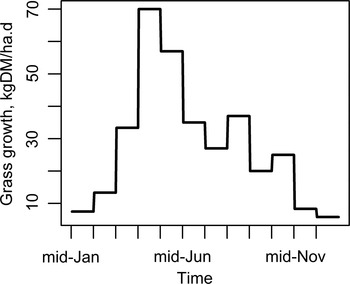
Fig. A1. Grass growth (kgDM ha−1 day−1) in western Pyrénées during the year.
Appendix B
MORRIS ANALYSIS OF THE ANIMAL SURVIVAL TRAITS
See Figure B1

Fig. B1. Scatter plots of the two sensitivity measures of Morris method, μ* (mean of absolute deviations of the elementary effects) and σ (standard deviation of the elementary effects), of the 27 model parameters for the model output of mortality during lamb period (A), and associated date of survival (B), and then for the model output of mortality during ewes period (C) and associated date of survival (D). Dashed boxes represent 50% of the parameter with the highest μ* and 50% of the parameter with the highest σ.


 Open access