


Introduction
Metal–Silicate Partitioning Experiments and the Composition of the Core
Core formation occurs during planetary accretion as a result of the planet's metallic core segregating from its silicate mantle at the base of one or more planet-wide magma oceans (Rubie et al., Reference Rubie, Frost, Mann, Asahara, Nimmo, Tsuno, Kegler, Holzheid and Palme2011). In order to unravel the conditions these processes occur under, a robust predictive model for the partitioning of various elements between silicate and metallic liquids is required (e.g., Jones & Drake, Reference Jones and Drake1986; Rubie et al., Reference Rubie, Gessmann and Frost2004, Reference Rubie, Frost, Mann, Asahara, Nimmo, Tsuno, Kegler, Holzheid and Palme2011; Wood et al., Reference Wood, Walter and Wade2006). Likewise, because planetary core compositions cannot be directly measured, only inferred from geophysical data, a better understanding of partitioning behavior at high pressure and temperature can be used to model the composition of Earth's core.
Experimental studies typically examine partitioning of various elements between liquid metal and silicate melt. These are performed at high temperature (T) (>1500 K) over a range of experimentally accessible pressures (P) in piston–cylinder or multi-anvil apparatus, and measured by an electron probe microanalyzer (EPMA) and/or laser-ablation–inductively coupled plasma–mass spectrometry (LA–ICP–MS). Both siderophile elements (Ni, Co, and others: e.g., Li & Agee, Reference Li and Agee1996; Righter et al., Reference Righter, Drake and Yaxley1997; Geßmann & Rubie, Reference Geßmann and Rubie1998) and light elements (e.g., Kilburn & Wood, Reference Kilburn and Wood1997; Gessmann et al., Reference Gessmann, Wood, Rubie and Kilburn2001; Dasgupta et al., Reference Dasgupta, Chi, Shimizu, Buono and Walker2013; Tsuno et al., Reference Tsuno, Frost and Rubie2013) partitioning have traditionally been examined in this way. Following the initial study of Bouhifd & Jephcoat (Reference Bouhifd and Jephcoat2003), the use of diamond anvil cell (DAC) experiments to access higher PT conditions, more relevant for core formation in large bodies, has become increasingly common for examining both siderophile and lithophile element partitioning. It is noted from such experiments that pressure trends obtained from the larger volume, lower pressure experiments do not always extrapolate with those identified at much higher pressures in DAC experiments (e.g., Suer et al., Reference Suer, Siebert, Remusat, Menguy and Fiquet2017). At the very high PT conditions achievable in a DAC, light elements in particular may become much more compatible in liquid iron (e.g., Frost et al., Reference Frost, Asahara, Rubie, Miyajima, Dubrovinsky, Holzapfel, Ohtani, Miyahara and Sakai2010), suggesting that some elements that are traditionally thought of as entirely incompatible in metal may be present in Earth's core in non-negligible concentrations (e.g., Badro et al., Reference Badro, Siebert and Nimmo2016; Blanchard et al., Reference Blanchard, Siebert, Borensztajn and Badro2017).
Analytical Considerations
DAC experimental sample volumes are orders of magnitude smaller than even the highest pressure multi-anvil experiments (around ~0.0001 mm3 for DAC experiments, compared with ~1 mm3 for multi-anvil products). The compositions of experimental run products are typically measured by WDS (wavelength-dispersive spectroscopy) by EPMA (Bouhifd & Jephcoat, Reference Bouhifd and Jephcoat2003, Reference Bouhifd and Jephcoat2011; Siebert et al., Reference Siebert, Badro, Antonangeli and Ryerson2012, Reference Siebert, Badro, Antonangeli and Ryerson2013; Badro et al., Reference Badro, Siebert and Nimmo2016; Blanchard et al., Reference Blanchard, Siebert, Borensztajn and Badro2017; Jackson et al., Reference Jackson, Bennett, Du, Cottrell and Fei2018; Mahan et al., Reference Mahan, Siebert, Blanchard, Borensztajn, Badro and Moynier2018) or energy-dispersive spectrometry (EDS) (Chidester et al., Reference Chidester, Rahman, Righter and Campbell2017). Other techniques commonly utilized include scanning transmission electron microscopy ((S)TEM mapping) or electron energy loss spectroscopy (EELS) and nanoscale secondary ion mass spectrometry (SIMS) (e.g., Frost et al., Reference Frost, Asahara, Rubie, Miyajima, Dubrovinsky, Holzapfel, Ohtani, Miyahara and Sakai2010; Fischer et al., Reference Fischer, Nakajima, Campbell, Frost, Harries, Langenhorst, Miyajima, Pollok and Rubie2015; Suer et al., Reference Suer, Siebert, Remusat, Menguy and Fiquet2017), which usually require at least major element analyses performed by scanning electron microscopy (SEM) or EPMA-based techniques if they are to yield fully quantifiable element data. The small size of DAC samples necessitates their preparation for SEM and EPMA analysis. This is most frequently achieved by cutting and removing a 1–4 µm thick slice by focused ion beam (FIB). Such a double-polished lamella has the advantage of confirming that the metal ball is sectioned at its widest point such that the interface between the two phases will be as close as possible to 90° from the polished surface, which reduces the risk of secondary fluorescence from subsurface metal or silicate. In addition, it allows for easy follow-up study by TEM techniques following further thinning. Alternative preparation methods include slicing perpendicular to the culets on a single side by FIB (e.g., Jackson et al., Reference Jackson, Bennett, Du, Cottrell and Fei2018) or polishing or slicing parallel to the diamond culets (e.g., Bouhifd & Jephcoat Reference Bouhifd and Jephcoat2003, Reference Bouhifd and Jephcoat2011), which both have the advantage of producing a thicker sample, but do not guarantee that a material is homogeneous throughout its depth. The DAC experiments using metal–silicate mixtures tend to segregate into a central metal ball (~5–10 µm diameter) and a quenched silicate melt rim of ~1–5 µm thickness surrounded by unmelted starting material. This study focuses on WDS measurement by EPMA, where attainable detection limits are in the region of 100 ppm, but conclusions are equally applicable to fully standardized EDS measurement by SEM, where detection limits are typically ~0.1 wt%.
The small sample size and geometry presents unique analytical challenges: a primary requirement for quantitative electron beam analysis is that both standards and unknowns are geometrically identical and homogenous on the scale of the analysis. These requirements are especially problematic in DAC experiments where element partitioning between coexisting chemically and physically dissimilar phases is desired (Wade & Wood, Reference Wade and Wood2012). Experiments focused on the conditions of terrestrial core formation, and the partitioning of elements between metallic and silicate phases, typically utilize analytical accelerating voltages (V acc) of either 15 or 20 kV. The choice of V acc is ultimately determined by the highest energy X-ray line being analyzed, with the rule-of-thumb being to use a minimum of twice the critical excitation of the highest energy line if good counting statistics are required. Given that a focused 15 kV electron beam impinging on iron will generate an analytical volume approximately 1 µm in diameter, an immediate concern is the sample thickness, where electrons may be lost through the underside of the sample, decreasing the apparent X-ray yield. A direct interaction with a second, chemically distinct, phase may also occur close to a material interface.
In addition, secondary fluoresced X-rays can be generated by excitation both by primary and continuum X-rays possessing energies above the critical excitation edge, which may occur at significant distances (tens of μm) from the point of analysis (Green, Reference Green1964). Although these usually account for just a negligible percentage of total measured X-rays, their proportion becomes significant when measuring trace concentrations of a given element close to an interface where the concentration is much higher in the adjacent phase (e.g., Dalton & Lane, Reference Dalton and Lane1996; Borisova et al., Reference Borisova, Zagrtdenov, Toplis, Donovan, Llovet, Asimow, De Parseval and Gouy2018). In particular, Wade & Wood (Reference Wade and Wood2012) point out that siderophile element partitioning experiments may have artificially elevated counts from the element of interest in the silicate phase, where both X-ray concentrations and absorption are low, allowing fluoresced X-rays originating from the metal to travel relatively unimpeded. The problems of spurious analyses in DAC experiments are exacerbated at higher accelerating voltages, where significant continuum radiation exists above the critical excitation edge of the highest energy lines typically analyzed (Ni and Cu).
EPMA is still the most widely used technique for obtaining publishable compositions of DAC experiments—it offers rapid, fully quantified analyses at micron scale spatial resolutions, combined with low relative errors (<2%). Typically, analyses utilize a ‘standard’ 15 or 20 kV setup, with minimal consideration given to analytical artifacts which may affect the measurements of such small samples. We present here a detailed extension of the initial study of Wade & Wood (Reference Wade and Wood2012), where we test and quantify limitations from (a) sample thickness and (b) fluorescence across interfaces. We use both simulations and make real measurements of synthetic samples which are optimized to imitate the geometries of real DAC sample measurements. In doing so, we suggest recommendations for the measurement of real DAC experiments, and address whether offsets between DAC and multi-anvil partitioning trends are artifacts of the analytical method.
Materials and Methods
Preparation of Synthetic Samples
All manufactured samples are shown in Figure 1. In order to test the effects of thickness, wedge-shaped samples with dimensions similar to DAC sample lamellae were cut by Ga-source FIB at the Bayerisches Geoinstitut (Universität Bayreuth, Germany) and welded onto copper TEM sample holders using Pt deposition. A metal alloy sphere (85 wt% Fe, 5 wt% Ni, 5 wt% Mo, 5 wt% W) was synthesized using an aerodynamic levitation set-up coupled with CO2 laser heating at the CEMTHi (Orleans, France). The levitation chamber was first vacuum pumped and the metal powder kept in levitation in a purified argon flow, avoiding any oxidation during the melting at about 1600°C. A thin wedge [Exp1] (Fig. 1) of a polished surface of the metal sphere was extracted using the FIB. A silicate wedge [Exp2] (Fig. 1) was cut from a polished synthetic CFMAS basalt [after 1.5 GPa eutectic CMAS composition of Presnall et al. (Reference Presnall, Dixon, Dixon, O'Donnell, Brenner, Schrock and Dycus1978) plus Fe2O3: 13.0 wt% MgO, 22.4 wt% Al2O3, 46.4 wt% SiO2, 11.2 wt% CaO, 5.1 wt% Fe2O3], which had been synthesized by melting a well-ground mixture of high-purity oxide powders at 1600°C in a box furnace. In both cases, a wafer of 10 × 20 × 3 µm was initially cut and lifted out of the material and welded to the copper holder with platinum. The wedges were then cut to be around 1 µm at the thinnest point, with a thick post retained on either side for stability.
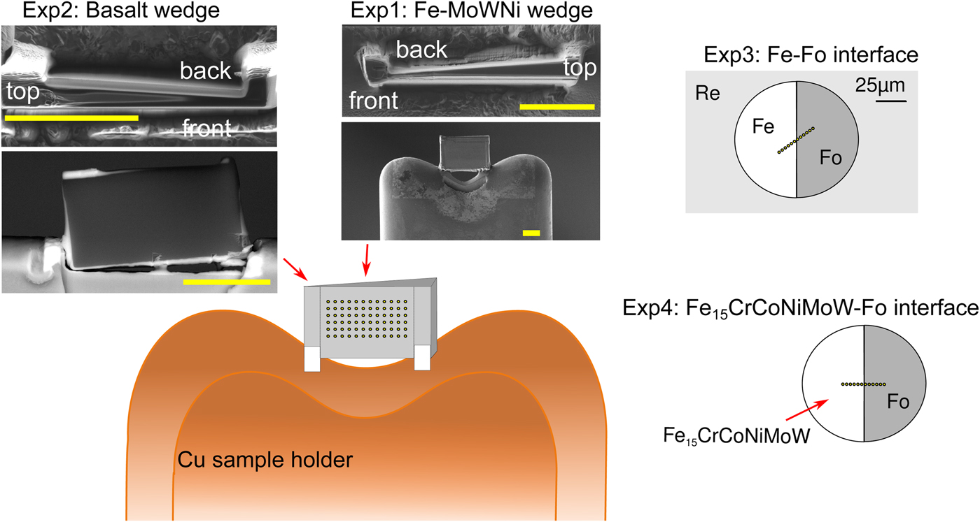
Fig. 1. Graphical overview of the experiments performed for this study, and positions of the analytical points. [Exp1–2] were cut by FIB and welded to Cu TEM lift-out grids using Pt, with the grids mounted flat for EPMA measurement. For these experiments, the measurements were performed by averaging over grids of analytical points, as illustrated. The simulations did not include the Cu grids or Re gasket. [Exp1]: Wedge of Fe85Ni5Mo5W5 (weight proportions); simulation and measurement. [Exp2]: Wedge of CFMAS basalt; simulation and measurement. [Exp3]: Fe–forsterite interface, measurements along a transect, simulation and measurement. [Exp4]: Fe15CrCoNiMoW–forsterite interface, simulation only.
For the interface (synthetic grain boundary) experiments, materials were mechanically pressed together without the use of heat, ensuring no reaction between the coexisting phases. Pure Fe and pure powdered forsterite (Fo) crystal with a straight interface were forced together in a DAC [Exp3] (Fig. 1). For this, diamonds with 250 µm culets were used with a 200 µm thick Re gasket. Following pre-indentation to 50 µm thickness, a 90 µm diameter chamber was cut in the gasket center by a laser. Fe foil was placed in the chamber, compressed, and decompressed. A semicircle was cut out using the using the laser drilling system at the Bayerisches Geoinstitut, and the edge neatened by FIB. The remaining space was then filled by Fo powder. The cell was then compressed to around 15 GPa to remove all pore space from the powder and give the optical impression of a homogeneous glass. The gasket was then mounted flat in epoxy and carefully polished to expose the grain boundary with no surrounding topography (Fig. 1).
Measurement
Samples were attached as wafers on copper holders and mounted flat in clamps in a custom holder for EPMA analysis, with sloped surfaces and topography from the support stems facing downward so that emitted X-rays emerged from a flat surface. Analyses were performed using a JEOL JXA 8200 EPMA at the University of Bayreuth using a 15 kV, 15 nA focused beam for the metal wedge and interface experiments, and a 1 µm diameter beam for the silicate glass wedge. Grids of measurement points were used to improve statistics, except for [Exp3], where a low-angle transect was measured. Typical polished standards appropriate to the material were chosen (all metals for the metal; olivine, diopside, and andradite for the silicate). Cu was also measured, and Cu fluorescence from the holder was found to be significant. Measured and simulated lines for most elements were Kα1. Lα1 was used for Mo. W was measured using Lα1 with long counting times. Because it is preferable to measure the lower energy W Mα1 at 15 kV when Si is not present, we tracked both W Lα1 and W Mα1 in simulations for comparison. The default JEOL Φ(ρz) correction (metal: XPP, Pouchou & Pichoir, Reference Pouchou and Pichoir1991; oxide: Love et al., Reference Love, Cox and Scott1978; Armstrong, Reference Armstrong1991) was applied and oxygen in silicates was assigned by stoichiometry.
Simulations
Monte Carlo simulations were performed using the simulation package PENEPMA (v. 2014; Llovet & Salvat, Reference Llovet and Salvat2017). PENEPMA simulates the geometry of a typical EPMA analysis, in addition to the electron transport and resultant X-ray generation within electron-irradiated materials. It uses the general-purpose PENELOPE code (Salvat, Reference Salvat2015) optimized for EPMA-type applications. Here, materials, geometry, simulation parameters, and the position of the detectors can be defined and the energy, origin, mechanism (e.g., primary, Bremsstrahlung, secondary fluorescence), and trajectories of generated X-rays are tracked to mimic a real EPMA measurement. By simulating the X-ray yield from both mono-phase standards and unknowns with complex, multi-phase geometries, fully quantified simulations may be performed. The high degree of accuracy of such Monte Carlo simulations has been previously demonstrated by comparing simulations with EPMA measurements for a wide range of materials (Llovet et al., Reference Llovet, Pinard, Donovan and Salvat2012, and references therein; Borisova et al., Reference Borisova, Zagrtdenov, Toplis, Donovan, Llovet, Asimow, De Parseval and Gouy2018). In this study, we simulate the same experiments that are measured by EPMA [Exp1–3] (Fig. 1), which allows the validity of the simulations to be checked. We additionally simulate a fictional interface between an alloy of Fe15NiCoCrMoW and forsterite [Exp4] (Fig. 1).
Although PENEPMA can be used to simulate the detector geometry of an EPMA (e.g., realistic spectrometer positions and window sizes), such a realistic simulation is not feasible due to the extremely low count efficiency (i.e. the likelihood of a single X-ray having the correct 3D trajectory to reach the spectrometer is tiny) and this results in extremely long calculation times. As a compromise between efficiency and realistic geometry, we follow the approach of Wade & Wood (Reference Wade and Wood2012) and use an annular (360°) detector with a 35–45° vertical extent. This is based on the typical 40° take-off angle in microprobes, and the assumption that X-ray trajectories will have randomly distributed horizontal components. Although not strictly true, this is always assumed in EPMA measurements, and the reduction in accuracy from angular inhomogeneity was found to be small by Wade & Wood (Reference Wade and Wood2012). Tests indicate that increasing the annular detector from 1 to 10° about the 40° take-off angle drastically increased counting efficiency while negligibly affecting results. To reduce run times, the following steps were taken: (i) low energy cut-offs were applied just below the lowest energy X-ray line of interest; (ii) the elastic scattering simulation parameters C 1 and C 2 were set to 0.05; and (iii) interaction forcings were applied to increase the likelihood of interactions (see Llovet & Salvat, Reference Llovet and Salvat2017, Reference Llovet and Salvat2018). The resulting small loss in accuracy should not noticeably affect the results (Llovet & Salvat, Reference Llovet and Salvat2018).
K-ratios (the ratio of X-ray counts from unknowns to X-ray counts of standards) were determined by simulating large standards, essentially infinitely thick with respect to the electron beam, of the same synthetic composition as the unknowns (materials of interest), with the same conditions and detector geometries. The default Armstrong/Love Scott Φ(ρz) correction was applied to the outputs using the software CalcZAF (derived from CITZAF; Armstrong, Reference Armstrong1995; using the FFAST mass absorption coefficients) to convert K-ratios to concentrations, mimicking the microprobe data treatment. A 15 kV simulation of Fe10SiO2 was converted to composition differently to the other runs, by using simulated SiO2 and Fe standards: this was done to assess the effect of choice of correction routine on the results.
Results
Thickness
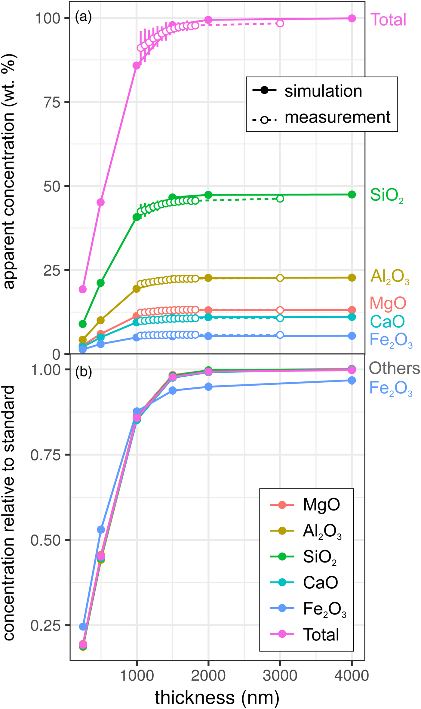
Measurements and simulations across the Fe85Ni5Mo5W5 (weight proportions) metal wedge [Exp1] are shown in Figures 2a and 2b, and show the measured and simulated concentrations at two scales. Over the range of thicknesses measured (900–2300 nm), there is no clear systematic change in elemental concentrations measured by EPMA, which is in good agreement with the simulations. In the simulations, apparent concentrations sum to around 99.6% at 4000 nm and decrease as the sample thins, although a strong drop-off is only observed when the metal is thinner than 500 nm, which reflects a truncation of the primary interaction volume. In pure Fe, the depth over which 95% of interactions occur reaches a maximum of ~530 nm; electrons are lost from the base of samples thinner than this, leading to a difference in the interaction volumes between the thick standards and the thinned sample. Figure 2c shows the simulated apparent concentrations as a proportion of the thick standard. Where the primary excitation volume is truncated (e.g., in the 250 nm sample), the intensities of the various X-ray lines are unequally diminished, with the higher energy X-ray lines apparently reduced to a greater extent. This results in erroneous measured elemental ratios, and implies that measurements of thin samples cannot be easily normalized to 100% without introducing non-systematic errors. Fe-rich alloys can be analyzed with an accelerating voltage of 15 kV to a thickness of around 1000 nm, which is thinner than DAC samples are typically prepared, without introducing significant analytical errors. However, TEM wafers, typically of approximately 200 nm thickness, require appropriate standards of the same thickness if they are to be analyzed by EPMA, or a thin film correction must be applied.
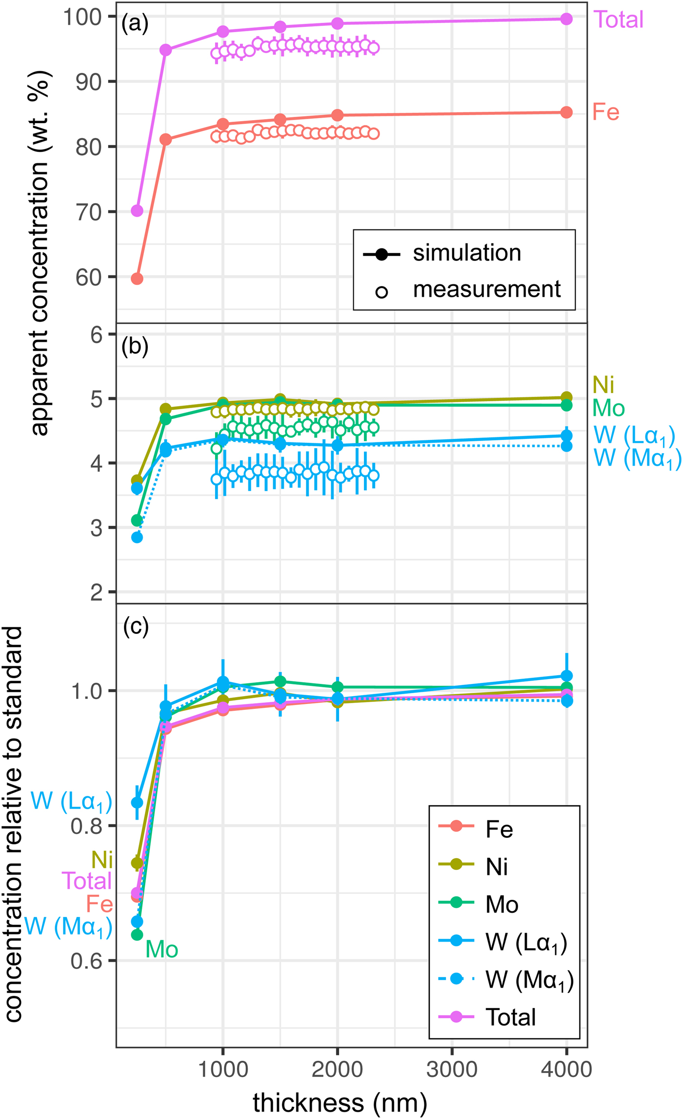
Fig. 2. Simulations and EPMA measurements along a metal Fe85Ni5Mo5W5 wedge [Exp1], showing apparent concentration as a function of thickness. Open symbols are measurements, closed are simulated points (if not visible, error bars are smaller than the symbol). All uncertainties are 2σ: in simulations, they are based on counting statistics and in measurements they are the standard deviation of repeat analyses on the reference Fe85Ni5Mo5W5 metal standard. Dotted line shows WMα1 as an alternative to WLα1. a: Fe and total wt%; b: Ni, Mo, and W (note change in scale); and c: simulated concentrations divided by their concentration in a simulated thick Fe85Ni5Mo5W5 standard.
Results for the synthetic basalt wedge measurement and simulation [Exp2] are shown in Figure 3. Uncertainties in the EPMA measurements shown here result from a taper in the wedge, typical of sections prepared by FIB cutting, and the resultant uncertainty in thickness measurement (to a lesser extent, this is also the case for the metal wedge results [Exp1]). The effect of reduced thickness on the apparent concentrations is more pronounced than for the metal: X-ray production reduces noticeably at 1500–2000 nm in both simulation and EPMA measurement. This results from the lower mean atomic number and density of the basalt (~3 g/cm3) in comparison with the metallic sample (7.8 g/cm3), and hence the lower electron stopping power and the larger resultant interaction volume. The drop-off in X-ray intensity is significant: at <1500 nm, silicate samples are not analyzable using standard analytical routines with any degree of confidence. However, unlike in the metal sample, ratios of oxides are approximately preserved (Fig. 3b). Although the electron interaction volumes are truncated, the relative differences in the interaction volumes of typical silicate forming elements are not significantly different (barring iron). This results in analyses of thin Fe-free silicate samples preserving element ratios, while absolute concentrations are erroneous. However, if Fe is present, one cannot simply scale to 100 wt%. The consistency of the EPMA measurements with the simulations in Figure 3 shows that simulations are an effective method to test for the presence of thickness-related analytical problems when working with FIB-prepared DAC experiments. When measuring glasses containing other trace elements (e.g., Chidester et al., Reference Chidester, Rahman, Righter and Campbell2017) using routine EPMA analytical conditions, simulations can reveal if element ratios are preserved.

Fig. 3. Simulations and EPMA measurements along a synthetic CFMAS basaltic glass wedge [Exp2], showing apparent concentration as a function of thickness. Symbols and uncertainty as described for Figure 2. a: Apparent concentration (wt%) of all oxides and oxide total; and b: simulated concentrations divided by those from a simulated thick standard.
Secondary Fluorescence
The Metal–Silicate Interface
X-ray fluorescence across the metal–silicate interface was examined with two experiments. The first was a planar interface between forsterite and pure iron [Exp3], which was both measured and simulated: the results are shown in Figure 4, and the spatial distribution of the origin of secondary fluoresced X-rays is shown in Figure 5. The measurements and simulations closely match one another, in agreement with previous comparative studies (Llovet & Salvat, Reference Llovet and Salvat2017, and references therein). The second simulation is of a planar interface between pure forsterite and a Fe15NiCoCrMoW metal ([Exp4], Fig. 1).
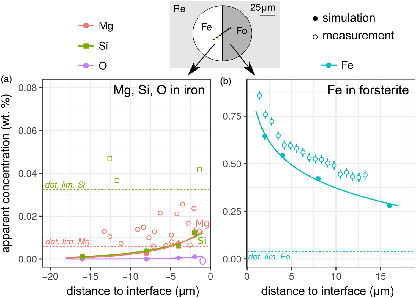
Fig. 4. Simulations and EPMA measurements along a transect across a forsterite–Fe metal interface [Exp3]. The transect was made at an angle to increase spatial resolution: plotted distances have been corrected to be normal to the interface. Symbols and uncertainties as for Figure 2. a: Apparent Si, Mg, and O (simulation only) wt% concentrations on the metal side; and b: apparent Fe concentrations on the forsterite side. Curves are exponential fits to the data. Si and Mg apparent concentrations are only shown above their detection limits. Note the dramatically different y-axis scale in the two plots.

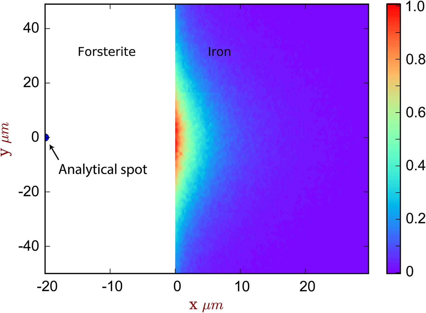
Fig. 5. The spatial distribution of sites of secondary fluoresced X-ray generation projected into two dimensions (integrated through z), corresponding to the simulation of [Exp3] and Figure 4. The analytical spot is in forsterite, 20 µm from the interface with iron. The color scale is relative, showing a proportion of the maximum intensity generated. Note that this figure shows X-ray generation and is not corrected for absorption.
Contamination of metal analyses by spurious signal from lithophile elements is usually assumed to be negligible, given the high density and mean atomic number of the metal, and the consequent greater attenuation of soft X-rays. Wade & Wood (Reference Wade and Wood2012) found extremely low concentrations of Si and O in simulations of a 10 µm diameter metal ball in basaltic glass. Our simulations and measurements confirm this, an apparent concentration of 0.007 wt% each of Mg and Si would be measured in iron at a distance of 5 µm from the interface with forsterite (Fig. 4a), which is below the detection limit of the EPMA measurements made here. Fluorescence of oxygen from the neighboring silicate phase (here simulation only) is effectively non-existent; the low energy O Kα1 X-rays are efficiently absorbed.
The contribution of fluoresced X-rays from the metal in the forsterite measurement is significantly higher. Figure 5 indicates that these secondary X-rays are generated from up to around 5 µm depth in the metal, but are concentrated along the interface. Figure 4b shows the apparent Fe concentration in forsterite. The measurements and simulation show the same trend and curvature, but have a small offset. This simulation–analysis offset may be attributed to the difference in real and simulated spectrometer positions with respect to the boundary and any attendant spectrometer defocusing arising from the boundary's position with respect to the spectrometer's focal line. Simulation and analyses reveal the same magnitude of effect: at a distance of 5 µm from the Fe:Fo interface, around 0.5–0.6 wt% Fe (0.64–0.77 wt% FeO) would be erroneously detected in pure forsterite. Luckily, DAC partitioning experiments are apparently rather oxidizing, and FeO measured in the silicate portions can be as high as 30 wt% (e.g., Blanchard et al., Reference Blanchard, Siebert, Borensztajn and Badro2017), so this fluorescence would only slightly increase the apparent  $f_{{\rm O}_{\rm 2}}$ and distribution coefficient K D (the ratio of partition coefficient of the element of interest to that of Fe). Conversely, primary and secondary X-rays from the sub-μm suspended metallic droplets that are often observed in the silicate may contribute more to the overestimation of FeO contents in the silicate glass than fluorescence from the large metallic ball.
Figure 6 shows the simulated results of fluorescence arising from an iron alloy (Fe15NiCoCrMoW) adjacent to the analyzed forsterite. In addition to the high fluorescence contribution from Fe, there is also a contribution from the other elements present. Figures 6a and 6b show the apparent measured concentrations; it should again be noted that these data will be typically interpreted as oxides, and should be scaled accordingly. As expected, the lowest energy lines, Mo (Lα1) and W (Mα1), exhibit the lowest contribution arising from fluorescence relative to the other minor elements. This demonstrates both the value in using lower energy lines to avoid fluorescence issues, and the advantages in performing analyses at lower accelerating voltage and concomitant decrease in high-energy continuum X-rays.
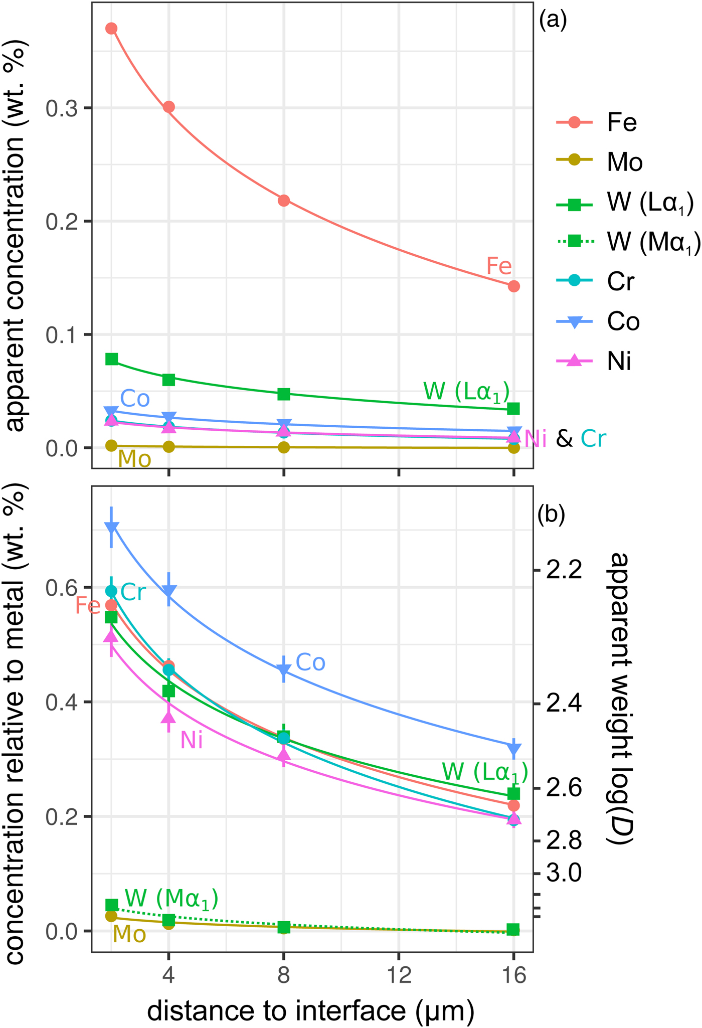
Fig. 6. Simulations along a transect from a forsterite–metal (Fe15CrCoNiMoW) interface [Exp4], showing points in the forsterite side only. Uncertainties and curves as in Figure 4. Dotted line shows WMα1 as an alternative to WLα1; in (a) it is identical to the curve for Mo and thus is not visible. a: Apparent concentrations in the forsterite, as a function of distance from the interface with the metal. b: Concentrations of the elements divided by their concentrations in a simulated metal Fe15CrCoNiMoW standard. Because the trace elements do not have equal weight concentrations in the metal, the fluoresced concentrations are also shown as percentages of the concentration in the metal.
Secondary Fluorescence and from Cu Holder
DAC partitioning experiments are almost universally prepared for analysis by cutting by FIB and welding to a Cu TEM sample holder with Pt. A high measured apparent concentration of Cu (Kα1) was detected in all of the samples of this study, despite them being Cu-free. Cu measurements from two experiments [Exp1 and 2] are shown in Figure 7. We observe that (i) the apparent Cu concentration is high (0.5–1.2 wt%), even at distances of over 20 µm from the Cu holder; (ii) Cu concentrations drop off with distance; and (iii) measurements of metal are more affected by Cu fluorescence than silicate. Although there is some uncertainty in Figure 7 caused by the sample holder shape, it is clear that Cu fluorescence is always problematic in DAC experiments, resulting from fluorescence by continuum X-rays and the relatively high energy and low attenuation of Cu Kα1.
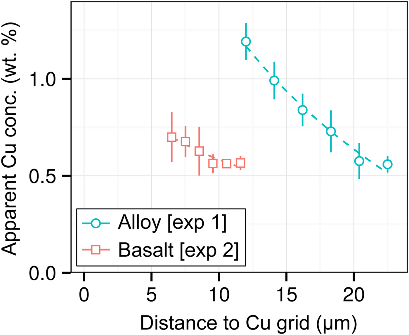
Fig. 7. Open symbols show apparent Cu concentrations (wt%) from EPMA measurements of the metal wedge [Exp1] (blue circles) and the basaltic glass wedge [Exp2] (red squares). In both cases, points are averages of measurements equidistant from the Cu holder, and error bars are the standard deviation. Relative distances between points in a series are accurate, although the absolute distance to the Cu holder has an uncertainty of a few micrometers due to the curved holder geometry and uncertain measurement grid placement. Dashed lines are exponential fits to the data.
Correction Procedure
The choice of correction routine used to convert K-ratios to concentrations is usually given little attention by end-users, because in typical microprobe measurements of geological materials, corrections tend to be small to moderate if appropriate standards—those of similar composition to the unknown—are used. However, there are no suitable oxygen-bearing iron standards available, because at 1 atmosphere, oxygen solubility in pure iron is very low. Hence, matrix extrapolations using pure iron and an oxide standard for O are potentially large; a light element with low-energy characteristic X-rays embedded in a dense metallic matrix will be strongly affected by absorption, requiring a large correction which may be on the order of a factor of two or more. Approximations and uncertainties in the correction can therefore significantly affect the apparent light element concentration in metals.
A simulation of Fe10SiO2 was converted to an apparent composition using simulated SiO2 and Fe standards, in order to assess the effect of choice of correction routine on the apparent light element content of a metal. It is seen in Figure 8 that the different algorithms can give significantly different estimates of light element content. Although the Fe concentrations only have small relative variations, these can significantly impact the microprobe total as the Fe content is high. Errors in the light element content estimates are striking in some cases. Some methods underestimate Si and O, whereas others overestimate. O estimates tend to be less inaccurate than Si. The default routine used in CalcZAF, Armstrong/Love Scott, underestimates Si and O the most, O by 9% relative, and Si by 5%. The commonly used XPP routine gives more acceptable results, and Love-Scott 1 performs the best for light elements in iron.
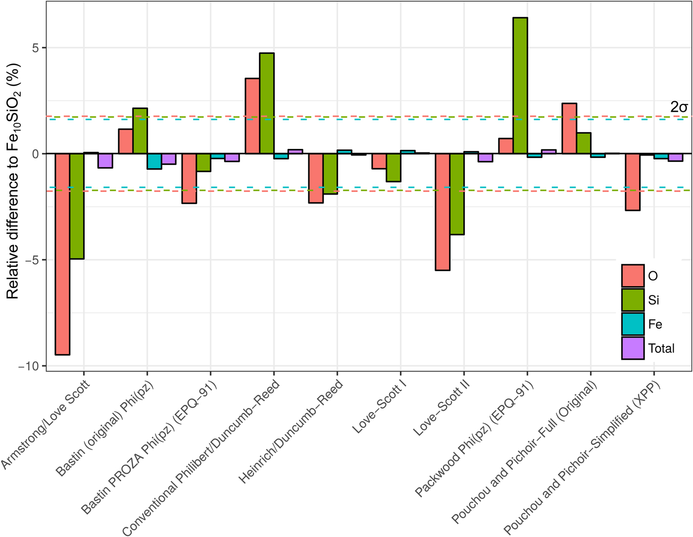
Fig. 8. Fe, Si, and O from a simulation of Fe10SiO2, where the simulated standards SiO2 and Fe were used with ten different correction routines in CalcZAF to calculate apparent concentrations. This is plotted as a percentage difference of the apparent composition from a given routine relative to Fe10SiO2.
Other Considerations
We note that earlier EPMA measurements of the metal wedge performed with our custom-made sample holder (which is hollow and adapts a JEOL thin section holder to fit FIB sample clamps) rotated by 180° were blighted by asymmetrical shadow effects. Topography is a common feature of DAC experiments because they are welded to three-dimensional, often custom made, sample holders, and workers should consider the increased risk of such effects. Primary signal from redeposited Cu and Pt in the FIB may also be responsible for a fraction of the signal in the case of low analytical totals, and we would also expect some fluorescence from the Pt welds. Re-deposition may additionally redistribute other elements, adding minor uncertainty to partitioning results, although careful cleaning with a low voltage Ga+ beam should reduce this issue.
Discussion
Secondary Fluorescence: Cause, Consequence, and Mitigation
Cause
Fluoresced X-rays are generated both by primary characteristic X-rays and continuum X-rays with energy above the fluoresced X-ray's critical excitation energy. As such, the lower attenuation of high-energy X-rays passing through a mixed material medium implies that the trace or minor element analyses may be compromised by spurious signals arising from neighboring phases. The attenuation of X-ray intensity with distance typically follows the Beer–Lambert law and is dependent both on material properties and X-ray energy. However, even by measuring as far as possible from the metal–silicate interface (e.g., 8 µm may be possible in some experiments), the analytical point is still well within the range of influence of secondary X-rays fluoresced in the neighboring phase, so increasing distance from the interface is not a practical solution. Instead, we recommend that analyses are checked with realistic simulations of both geometry and composition, the fluorescence contribution can then be effectively subtracted from an analysis. Problems are minimized for lower energy X-rays where attenuation within the metallic sample is significant. As such, lithophile elements in the metallic phase, such as Mg, Ca, and Al, tend to be less problematic, but strongly siderophile elements in silicate analyses such as Ni and Fe are compromised unless other mitigation is made in the analytical protocol (for instance, the analyses of lower energy lines or low over-voltage analysis). Caution should also be exerted when the partition coefficient is high and there is a large concentration difference between the two phases. Increasing the experimental doping of a trace element will only exacerbate the situation, but systematic errors can be minimized with the use of the simulation and subtraction method described here.
Consequence
The consequence of fluorescence across an interface in partitioning experiments, in any direction, is to reduce the concentration contrast between the two phases and bring the partition coefficient D closer to unity. To illustrate the pitfalls of neglecting the secondary fluorescence contribution, elemental concentration ratios may be used to calculate the apparent metal–silicate partition coefficient  $D_x^{{\rm met- sil}} $ where
 $$D_x^{{\rm met- sil}} = \; \displaystyle{{{\rm concentration\;} \,{\rm of}\,{\rm element}\,x\,{\rm in}\,{\rm metal}\;} \over {{\rm concentration}\,{\rm of}\,{\rm element}\,x\,{\rm in} \,{\rm silicate}}}\,{\rm (wt\%} )$$
 Figure 6b shows these displayed as the apparent log  $(D_x^{{\rm met- sil}} )$ if the silicate were completely devoid of that element. At 4 µm from the interface, Ni, Cr, and W have an apparent log $(D_x^{{\rm met- sil}} )$ of around 2.4, with Co below 2.3. In essence, this represents an upper limit on the measurement of siderophile behavior in the DAC; elements that possess a D met−sil in excess of ~250, and whose measured X-ray lines are of comparable energy with Fe, cannot be reliably measured by EPMA in the silicate from a typical DAC experiment. Most moderately siderophile elements at the oxidizing conditions typical of DAC experiments could reasonably be analyzed (ideally, subject to checking for possible fluorescence problems and applying a suitable data correction).
It is frequently noted that there is an offset in D between DAC experiments and extrapolated multi-anvil experiments. In these cases, fluorescence in the analyses should be considered as a possible cause. Wade & Wood (Reference Wade and Wood2012) found from a buried metal ball configuration that around 25% of the silicate NiO concentration of an experiment of Bouhifd & Jephcoat (Reference Bouhifd and Jephcoat2003) was fluoresced signal, and resulted in a significant underestimation of the siderophility of Ni. The Ni and Co partitioning data of Siebert et al. (Reference Siebert, Badro, Antonangeli and Ryerson2012) are somewhat offset to lower D (less siderophile) relative to previously published large volume experiments. This offset is explained by the authors as a strong pressure effect, where Ni is more compatible in silicate at core-forming conditions. In the current study, the secondary fluorescence contribution appears to be somewhat less than that of Wade & Wood (Reference Wade and Wood2012). If the measurements were made at a 4 µm distance from the interface, only 2–5% of NiO and CoO measured by Siebert et al. (Reference Siebert, Badro, Antonangeli and Ryerson2012) are from a fluoresced signal, meaning that the true log(K D) is only minimally higher than reported, then their conclusions are robust. We note that a curved interface from a thick slice of a sphere will somewhat increase fluorescence, which may be responsible for the difference between the level of fluorescence predicted in this study versus that of Wade & Wood (Reference Wade and Wood2012).
Mitigation
Ni and Co are only moderately siderophile, so caution is required for elements more siderophile than these, or for moderately siderophile elements in more reduced experiments (where D will be larger). In these cases, we recommend: (i) measuring a lower energy X-ray line (e.g., L or M lines, where appropriate, although concentrations may be too low to measure these effectively), and/or (ii) testing the problem by simulation and correcting for it. More siderophile elements may be off limits anyway, given the high levels of doping that would be required for a measurable quantity to be present in the silicate. Long counting times, high beam current and high dopant concentrations can help with counting statistics, but will make no difference in mitigating fluorescence. Using a 20 kV electron beam rather than a 15 kV one will increase the fluoresced contribution a little and increase the minimum allowable thickness (Wade & Wood, Reference Wade and Wood2012), so should be avoided.
Maximizing the analysis distance from a phase boundary obviously reduces the contribution arising from fluoresced X-rays (Fig. 6). However, practical considerations reduce the efficacy of this approach. The small experimental size of DAC runs limits this approach as an effective form of mitigation. Even measurements from large volume multi-anvil experiments may be compromised by fluorescence if concentrations in the silicate are too low and/or there is limited space for measurements to be made far from interfaces, typical in experiments performed in polycrystalline MgO capsules. DAC experiments also present other complications—they typically contain small metal droplets suspended in the silicate glass (Fischer et al., Reference Fischer, Nakajima, Campbell, Frost, Harries, Langenhorst, Miyajima, Pollok and Rubie2015; Blanchard et al., Reference Blanchard, Siebert, Borensztajn and Badro2017; Suer et al., Reference Suer, Siebert, Remusat, Menguy and Fiquet2017; Mahan et al., Reference Mahan, Siebert, Blanchard, Borensztajn, Badro and Moynier2018), a consequence of the high temperatures and inviscid nature of the coexisting liquids. This makes avoiding contributions from native metal and uncontaminated silicate analyses all the more difficult.
Low Totals in Published Metal Analyses
We note that published analyses of DAC metals frequently have low totals, whereas the analyses of the corresponding silicate phases are not low. In light of our results we would suggest that, with typical geometries, totals of 99% should be expected from a well-calibrated analysis (a deep fluoresced contribution of around 1% of Fe X-rays will be missing in 2000 nm thick samples). Totals as low as <95 wt% indicate problems other than the sample dimensions; their uncertain origin means that we cannot know that element ratios are correct. For example, problems in absorption corrections will disproportionately affect light elements in a denser iron matrix.
Conclusions
Metal–silicate partitioning studies performed by laser-heated DAC are increasingly being used to investigate siderophile and lithophile element distribution during core formation. However, the EPMA technique is being used at the limits of its capability when measuring these very small and thin samples. We investigate the limitations of such EPMA measurements in order to assess the validity of compositional measurements of partitioning experiments.
The results of our study generally support the published experiments to-date: samples in most (not all) studies are thick enough that their results should not be significantly affected by signal lost from the base of the sample. For 15 kV, we recommend a minimum sample thickness of 2000 nm to effectively analyze a quenched basaltic glass, although the metallic phase gives robust measurements at thicknesses greater than 1000 nm or less. Thicker samples will be required for 20 kV.
Fluorescence from metallic siderophile elements will contaminate the silicate measurement, but as long as the concentration contrast between metal and silicate is not too strong (log D ~ <2; i.e. moderately siderophile elements, or more siderophile elements at oxidizing conditions), fluoresced X-rays should only weakly increase the apparent concentration. We recommend simulating the fluorescence and applying a data correction, if required. Fluorescence from more strongly siderophile elements may only be mitigated by using a lower energy X-ray line, although concentrations will then likely be too low for a statistically reasonable signal, so DAC experiments may never be a suitable technique for measuring these. We caution that fluorescence can originate from sources external to the sample, as exemplified by the spurious >1 wt% of Cu that was observed in all samples welded to a Cu TEM grid.
Our results indicate that contamination of metal analyses by lithophile element fluorescence should be negligible. However, light lithophile element analyses in metals are difficult for other reasons. Their relatively low-energy X-rays are easily absorbed by the dense Fe matrix, and as such, large corrections must be applied to convert their K-ratios into concentrations. In this case, even the selection of correction routine can significantly affect the apparent composition, with relative concentration differences of up to 10% found by different correction procedures when using SiO2 as a standard. Choosing matrix-matched standards should reduce this difference, but the accuracy of the correction may additionally be affected by the heterogeneous texture that is frequently observed in the quenched metallic phase.
We find that simulated X-ray spectra using PENEPMA software are very consistent with real EPMA measurements, and so recommend the use of simple simulations as a reliable method to evaluate the extent to which data may be affected by artifacts in future experimental studies. Corrections could be calculated and reasonably applied, except in the case of siderophile elements, where microbeam analysis may not be appropriate.
Acknowledgments
We thank Ben Buse, Nobuyoshi Miyajima, and Katharina Marquardt for helpful discussion. We also thank an anonymous reviewer for useful comments that improved the clarity of our presentation, and Dr. Joseph Michael for editorial handling. We gratefully acknowledge financial support from the European Research Council (ERC) Advanced Grant ‘ACCRETE’ (Contract No. 290568). JW acknowledges receipt of an NERC Independent Research Fellowship NE/K009540/1. The FIB work at BGI was supported by DFG grant no. INST 91/315-1 FUGG.


 Open access