


Impact statement
Sea-level rise is an important aspect of climate change, with potentially large consequences for coastal communities around the world. Sea-level change is therefore an active area of research that has seen many developments in the past decades. Based on the available research, the Intergovernmental Panel on Climate Change (IPCC) provides regular updates on sea-level projections which are used by policymakers and for adaptation planning. In this review, we compare the sea-level projections from different IPCC reports in the past 10 years and explain what has changed in the methods used and in the numbers presented. We also compare observed changes from the 2021 IPCC report to projected changes from the 2013 IPCC report, for the overlapping period 2007–2018, and find that they are highly consistent. Finally, we share some potential future research directions on improving sea-level projections.
Introduction
Present-day sea-level change (SLC) is primarily a consequence of human-induced climate change, which will impact people and communities all over the world. From a decision-making perspective, knowing how much the sea level will rise, and when, can help to decide which protective measures need to be taken at which point in time. Therefore, sea-level projections are among the most anticipated outcomes of the Intergovernmental Panel on Climate Change (IPCC) assessment reports (ARs). While sea-level extremes are also an important consideration for future coastal hazards, in this review we focus our attention on projections of mean sea level.
In the past 15 years, process-based sea-level projections (i.e., projections which use models to simulate the physical processes and interactions contributing to sea-level change) in the IPCC reports have developed from global-mean only (AR4, Meehl et al., Reference Meehl, Stocker, Collins and Zhao2007) to regional projections (AR5, Church et al., Reference Church, Clark, Cazenave, Gregory, Jevrejeva, Levermann, Merrifield, Milne, Nerem, Nunn, Payne, Pfeffer, Stammer, Unnikrishnan, Stocker, Qin, Plattner and Midgley2013a). More recent reports focused on the Antarctic contribution (Special Report on Oceans and Cryosphere in a Changing Climate SROCC, Oppenheimer et al., Reference Oppenheimer, Glavovic, Hinkel, van de Wal, Magnan, Abd-Elgawad, Cai, Cifuentes-Jara, DeConto, Ghosh, Hay, Isla, Marzeion, Meyssignac and Sebesvari2019), and provided projections consistent with the assessed Equilibrium Climate Sensitivity (ECS) (AR6, Fox-Kemper et al., Reference Fox-Kemper, Hewitt, Xiao, Aðalgeirsdóttir, Drijfhout, Edwards, Golledge, Hemer, Kopp, Krinner, Mix, Notz, Nowicki, Nurhati, Ruiz, Sallée, Slangen, Yu, Masson-Delmotte, Zhai, Pirani and Zhou2021a). The research community has dedicated significant research effort and published many papers on improving the understanding and modelling of the different contributions to SLC, such as ice sheets, glaciers and sterodynamic changes (e.g., Gregory et al., Reference Gregory, Bouttes, Griffies, Haak, Hurlin, Jungclaus, Kelley, Lee, Marshall, Romanou, Saenko, Stammer and Winton2016; Nowicki et al., Reference Nowicki, Payne, Larour, Seroussi, Goelzer, Lipscomb, Gregory, Abe-Ouchi and Shepherd2016; The IMBIE Team, 2018, 2019; Hock et al., Reference Hock, Bliss, Marzeion, Giesen, Hirabayashi, Huss, Radic and Slangen2019). Since AR5, new global mean and regional projections have been published, using various methods: for instance based on fully coupled climate models (Slangen et al., Reference Slangen, Katsman, van de Wal, Vermeersen and Riva2012; Kopp et al., Reference Kopp, Horton, Little, Mitrovica, Oppenheimer, Rasmussen, Strauss and Tebaldi2014; Slangen et al., Reference Slangen, Carson, Katsman, van de Wal, Köhl, Vermeersen and Stammer2014a; Carson et al., Reference Carson, Köhl, Stammer, Slangen, Katsman, van de Wal, Church and White2015; Jackson and Jevrejeva, Reference Jackson and Jevrejeva2016; Buchanan et al., Reference Buchanan, Oppenheimer and Kopp2017; Palmer et al., Reference Palmer, Gregory, Bagge, Calvert, Hagedoorn, Howard, Klemann, Lowe, Roberts, Slangen and Spada2020), reduced-complexity models (Perrette et al., Reference Perrette, Landerer, Riva, Frieler and Meinshausen2013; Schleussner et al., Reference Schleussner, Lissner, Fischer, Wohland, Perrette, Golly, Rogelj, Childers, Schewe, Frieler, Mengel, Hare and Schaeffer2016; Nauels et al., Reference Nauels, Meinshausen, Mengel, Lorbacher and Wigley2017), semi-empirical models (Kopp et al., Reference Kopp, Kemp, Bittermann, Horton, Donnelly, Gehrels, Hay, Mitrovica, Morrow and Rahmstorf2016; Mengel et al., Reference Mengel, Levermann, Frieler, Robinson, Marzeion and Winkelmann2016; Bakker et al., Reference Bakker, Wong, Ruckert and Keller2017; Bittermann et al., Reference Bittermann, Rahmstorf, Kopp and Kemp2017; Goodwin et al., Reference Goodwin, Haigh, Rohling and Slangen2017; Wong et al., Reference Wong, Bakker, Ruckert, Applegate, Slangen and Keller2017; Jackson et al., Reference Jackson, Grinsted and Jevrejeva2018; Jevrejeva et al., Reference Jevrejeva, Jackson, Grinsted, Lincke and Marzeion2018), structured expert judgement (SEJ) (Bamber et al., Reference Bamber, Oppenheimer, Kopp, Aspinall and Cooke2019), or a mixture of methods (Grinsted et al., Reference Grinsted, Jevrejeva, Riva and Dahl-Jensen2015; Kopp et al., Reference Kopp, DeConto, Bader, Hay, Horton, Kulp, Oppenheimer, Pollard and Strauss2017; Le Bars et al., Reference Le Bars, Drijfhout and De Vries2017; Le Cozannet et al., Reference Le Cozannet, Manceau and Rohmer2017a). There have also been a number of reviews, including a database of sea-level projections (Garner et al., Reference Garner, Weiss, Parris, Kopp RE, Horton RM, Overpeck and Arbor2018), reviews on developments following AR5 (Clark et al., Reference Clark, Church, Gregory and Payne2015; Slangen et al., Reference Slangen, Adloff, Jevrejeva, Leclercq, Marzeion, Wada and Winkelmann2017a), overviews of processes and timescales (Horton et al., Reference Horton, Kopp, Garner, Hay, Khan, Roy and Shaw2018a; Hamlington et al., Reference Hamlington, Gardner, Ivins, Lenaerts, Reager, Trossman, Zaron, Adhikari, Arendt, Aschwanden, Beckley, Bekaert, Blewitt, Caron, Chambers, Chandanpurkar, Christianson, Csatho, Cullather, DeConto, Fasullo, Frederikse, Freymueller, Gilford, Girotto, Hammond, Hock, Holschuh, Kopp, Landerer, Larour, Menemenlis, Merrifield, Mitrovica, Nerem, Nias, Nieves, Nowicki, Pangaluru, Piecuch, Ray, Rounce, Schlegel, Seroussi, Shirzaei, Sweet, Velicogna, Vinogradova, Wahl, Wiese and Willis2020), reviews on coastal sea-level change (e.g., Van de Wal et al., Reference Van de Wal, Zhang, Minobe, Jevrejeva, Riva, Little, Richter and Palmer2019) and reviews integrating risk and adaptation assessments (e.g., Nicholls et al., Reference Nicholls, Hanson, Lowe, Slangen, Wahl, Hinkel and Long2021).
One thing that all sea-level projections have in common, despite the different approaches and methodologies, is an uncertainty that grows substantially through time. The uncertainties in regional sea-level projections over the coming years to decades result primarily from internal climate variability (see e.g., Palmer et al., Reference Palmer, Gregory, Bagge, Calvert, Hagedoorn, Howard, Klemann, Lowe, Roberts, Slangen and Spada2020, their Figure 11). On decadal to centennial timescales, uncertainties depend on the future forcings (such as greenhouse gas emissions) and the response of the climate system; and on the modelling uncertainty associated with simulating the different contributions to SLC. The forcing uncertainty can be assessed using different emissions or radiative forcing scenarios, varying from scenarios with net-zero CO2 emissions by 2050 to scenarios with a tripling of the present-day CO2 emissions by 2100. The modelling uncertainty can be relatively well quantified for some contributions, such as global mean thermal expansion. For other contributions, such as (multi)-century timescale ice mass loss of the Antarctic Ice Sheet, the uncertainty is characterised as ‘deep uncertainty’, which means that experts do not know or cannot agree on appropriate conceptual models or the probability distributions used (Lempert et al., Reference Lempert, Popper and Bankes2003; Kopp et al., Reference Kopp, Oppenheimer, O’Reilly, Drijfhout, Edwards, Fox-Kemper, Garner, Golledge, Hermans, Hewitt, Horton, Krinner, Notz, Nowicki, Palmer, Slangen and Xiao2022). These contributions are therefore a topic of much research and debate (e.g., Oppenheimer et al., Reference Oppenheimer, Glavovic, Hinkel, van de Wal, Magnan, Abd-Elgawad, Cai, Cifuentes-Jara, DeConto, Ghosh, Hay, Isla, Marzeion, Meyssignac and Sebesvari2019).
In addition to studies on future sea-level projections, much research has been focused on understanding past observations. A lot of progress has been made in the closing of the sea-level budget for the 20th century, which compares the sum of the observed contributions to the total observed changes, on global (e.g., Gregory et al., Reference Gregory, White, Church, Bierkens, Box, Van Den Broeke, Cogley JG. Fettweis, Hanna, Huybrechts, Konikow, Leclercq, Marzeion, Oerlemans, Tamisiea, Wada, Wake and Van De Wal2013; Chambers et al., Reference Chambers, Cazenave, Champollion, Dieng, Llovel, Forsberg, von Schuckmann and Wada2016; Cazenave et al., Reference Cazenave2018; Frederikse et al., Reference Frederikse, Landerer, Caron, Adhikari, Parkes, Humphrey, Dangendorf, Hogarth, Zanna, Cheng and Wu2020) and basin scales (e.g., Slangen et al., Reference Slangen, Van De Wal, Wada and Vermeersen2014b; Frederikse et al., Reference Frederikse, Riva, Kleinherenbrink, Wada, van den Broeke and Marzeion2016; Rietbroek et al., Reference Rietbroek, Brunnabend, Kusche, Schröter and Dahle2016; Frederikse et al., Reference Frederikse, Jevrejeva, Riva and Dangendorf2018; Wang et al., Reference Wang, Church, Zhang, Gregory, Zanna and Chen2021b). These budget studies have led to important advances in the understanding of sea-level change and its contributing processes on global and regional scales. In addition, the observations can be compared with model simulations (Church et al., Reference Church, Monselesan, Gregory and Marzeion2013c; Meyssignac et al., Reference Meyssignac, Slangen, Melet, Church, Fettweis, Marzeion, Agosta, Ligtenberg, Spada, Richter, Palmer, Roberts and Champollion2017; Slangen et al., Reference Slangen, Meyssignac, Agosta, Champollion, Church, Fettweis, Ligtenberg, Marzeion, Melet, Palmer, Richter, Roberts and Spada2017b; Oppenheimer et al., Reference Oppenheimer, Glavovic, Hinkel, van de Wal, Magnan, Abd-Elgawad, Cai, Cifuentes-Jara, DeConto, Ghosh, Hay, Isla, Marzeion, Meyssignac and Sebesvari2019) to test, understand and improve the model representation of the different processes. This has turned out to be challenging, especially for the earlier part of the 20th century: SROCC stated that only 51% of the 1901–1990 observed global mean sea-level (GMSL) change could be explained by models, due to ‘the inability of climate models to reproduce some observed regional changes’, in particular before 1970. The agreement between models and observations increased to 91% for 1971–2015 and 99% for 2006–2015 (Oppenheimer et al., Reference Oppenheimer, Glavovic, Hinkel, van de Wal, Magnan, Abd-Elgawad, Cai, Cifuentes-Jara, DeConto, Ghosh, Hay, Isla, Marzeion, Meyssignac and Sebesvari2019).
It is also possible to evaluate past projections against observations that have been made since. For instance, for total SLC, Wang et al. (Reference Wang, Church, Zhang and Chen2021a) found an almost identical GMSL trend in the observations and AR5 projections for the period 2007–2018. Lyu et al. (Reference Lyu, Zhang and Church2021) compared observations and climate model output of ocean warming for the purpose of constraining projections. They found a high correlation for the Argo period (2005–2019) and concluded that the observational record over this period is currently the most useful constraint for projections of ocean warming. Such evaluations against the already realised SLC are important to provide further insights and build confidence in sea-level projections.
Here, we will first discuss ‘how we got here’: recent methodological developments in process-based sea-level projections for the 21st century, with a brief recap of the IPCC sea-level projection methods up to IPCC AR5, followed by a discussion of the key differences between AR5, SROCC and AR6 projections (section ‘Key advances in sea-level projections up to IPCC AR6’). Next, we discuss ‘where we are’, by evaluating AR5 projections of SLC (which start from 2007 onwards) against observational time series (up to 2018), both for total GMSL and for individual contributions (section ‘Comparison of the AR5 model simulations with observations’). Finally, we discuss ‘where we’re going’: how can sea-level projections be better tailored for coastal information (section ‘Moving towards local information’). Throughout this review, we adopt the sea-level terminology defined by Gregory et al. (Reference Gregory, Griffies, Hughes, Lowe, Church, Fukimori, Gomez, Kopp, Landerer, Le Cozannet, Ponte, Stammer, Tamisiea and van de Wal2019) and we refer to Box 9.1 of IPCC AR6 (Fox-Kemper et al., Reference Fox-Kemper, Hewitt, Xiao, Aðalgeirsdóttir, Drijfhout, Edwards, Golledge, Hemer, Kopp, Krinner, Mix, Notz, Nowicki, Nurhati, Ruiz, Sallée, Slangen, Yu, Masson-Delmotte, Zhai, Pirani and Zhou2021a) for a summary of the key drivers of SLC.
Key advances in sea-level projections up to IPCC AR6
There have been substantial methodological and scientific advances in sea-level projections since the publication of the IPCC First Assessment Report in 1990 (Warrick and Oerlemans, Reference Warrick and Oerlemans1990). The use of global climate models (GCMs) in IPCC sea-level projections dates back to the IPCC Third Assessment Report (Church et al., Reference Church, Gregory, Huybrechts, Kuhn, Lambeck, Nhuan, Qin and Woodworth2001). In IPCC AR4, climate models from the third phase of the Climate Model Intercomparison Project (CMIP3) were used as the ‘backbone’ of the process-based GMSL projections (Meehl et al., Reference Meehl, Stocker, Collins and Zhao2007), with a similar approach adopted for AR5 using the CMIP5 generation of climate models (Church et al., Reference Church, Clark, Cazenave, Gregory, Jevrejeva, Levermann, Merrifield, Milne, Nerem, Nunn, Payne, Pfeffer, Stammer, Unnikrishnan, Stocker, Qin, Plattner and Midgley2013a). A major change for the AR5 was the inclusion of regional projections (following Slangen et al., Reference Slangen, Katsman, van de Wal, Vermeersen and Riva2012). The IPCC Special Report on Global Warming of 1.5° for the first time assessed GMSL based on warming levels (Hoegh-Guldberg et al., Reference Hoegh-Guldberg, Jacob, Taylor, Bindi, Brown, Camilloni, Diedhiou, Djalante, Ebi, Engelbrecht, Guiot, Hijioka, Mehrotra, Payne, Seneviratne, Thomas, Warren, Zhou, Masson-Delmotte, Zhai, Pörtner and Waterfield2018). The SROCC added new information on the dynamical ice sheet contribution to the AR5 projections (Oppenheimer et al., Reference Oppenheimer, Glavovic, Hinkel, van de Wal, Magnan, Abd-Elgawad, Cai, Cifuentes-Jara, DeConto, Ghosh, Hay, Isla, Marzeion, Meyssignac and Sebesvari2019). The main advance in AR6 was the use of physics-based emulators to ensure consistency of the sea-level projections with the AR6-assessed ECS and global surface air temperature (GSAT).
We will now discuss some of the key differences of the global mean and regional sea-level projections in IPCC AR6 relative to AR5 and SROCC, by explaining what has been done differently, why these changes were made, and what the effects are on the projections. We do not include the SR1.5 projections in this discussion (Hoegh-Guldberg et al., Reference Hoegh-Guldberg, Jacob, Taylor, Bindi, Brown, Camilloni, Diedhiou, Djalante, Ebi, Engelbrecht, Guiot, Hijioka, Mehrotra, Payne, Seneviratne, Thomas, Warren, Zhou, Masson-Delmotte, Zhai, Pörtner and Waterfield2018), as the SR1.5 report made a literature-based assessment of GMSL changes for 1.5° and 2°, but did not produce new projections.
Before we discuss the projections, we note that the interpretation and communication of the uncertainties in sea-level projections has varied across the different IPCC assessment reports (Kopp et al., Reference Kopp, Oppenheimer, O’Reilly, Drijfhout, Edwards, Fox-Kemper, Garner, Golledge, Hermans, Hewitt, Horton, Krinner, Notz, Nowicki, Palmer, Slangen and Xiao2022). IPCC reports use calibrated uncertainty language, in which the confidence level is a qualitative reflection of the evidence and agreement, whereas the likelihood metric is a quantitative measure of uncertainty, expressed probabilistically (Box 1.1, Chen et al., Reference Chen, Rojas, Samset, Cobb, Diongue Niang, Edwards, mori, Faria, Hawkins, Hope, Huybrechts, Meinshausen, Mustafa, Plattner, Tréguier, Masson-Delmotte, Zhai, Pirani and Zhou2021). For the medium confidence projections in AR5, the 5–95th percentile range of the model ensemble was interpreted as the likely range (the central range with about two-thirds probability, 17–83%), with the uncertainty range of all contributions inflated relative to the model spread to account for structural uncertainties arising from the CMIP5 model ensemble. For the sea-level projections in AR6 (Fox-Kemper et al., Reference Fox-Kemper, Hewitt, Xiao, Aðalgeirsdóttir, Drijfhout, Edwards, Golledge, Hemer, Kopp, Krinner, Mix, Notz, Nowicki, Nurhati, Ruiz, Sallée, Slangen, Yu, Masson-Delmotte, Zhai, Pirani and Zhou2021a, Section 9.6), the likely range was redefined as the central range with at least two-thirds probability, encompassing the outer 17th to 83rd percentiles of the probability distributions considered in a p-box (e.g., Le Cozannet et al., Reference Le Cozannet, Manceau and Rohmer2017a). That is, the definition of likely range in AR5, SROCC and AR6 is comparable but not exactly the same, and the way of determining the range from the available information is different. The AR6 medium confidence projections include estimated distributions for each emissions scenario with two different methodological choices for the Antarctic ice sheet (see Table 1). AR6 also presented a set of lowconfidence projections, which include additional contributions from ice sheet processes and estimates for which there is less agreement and/or less evidence (see Table 1).
Table 1. High-level summary of the methods used in the AR5, SROCC and AR6 reports to project global mean and regional SLC (1° × 1° resolution) to 2100
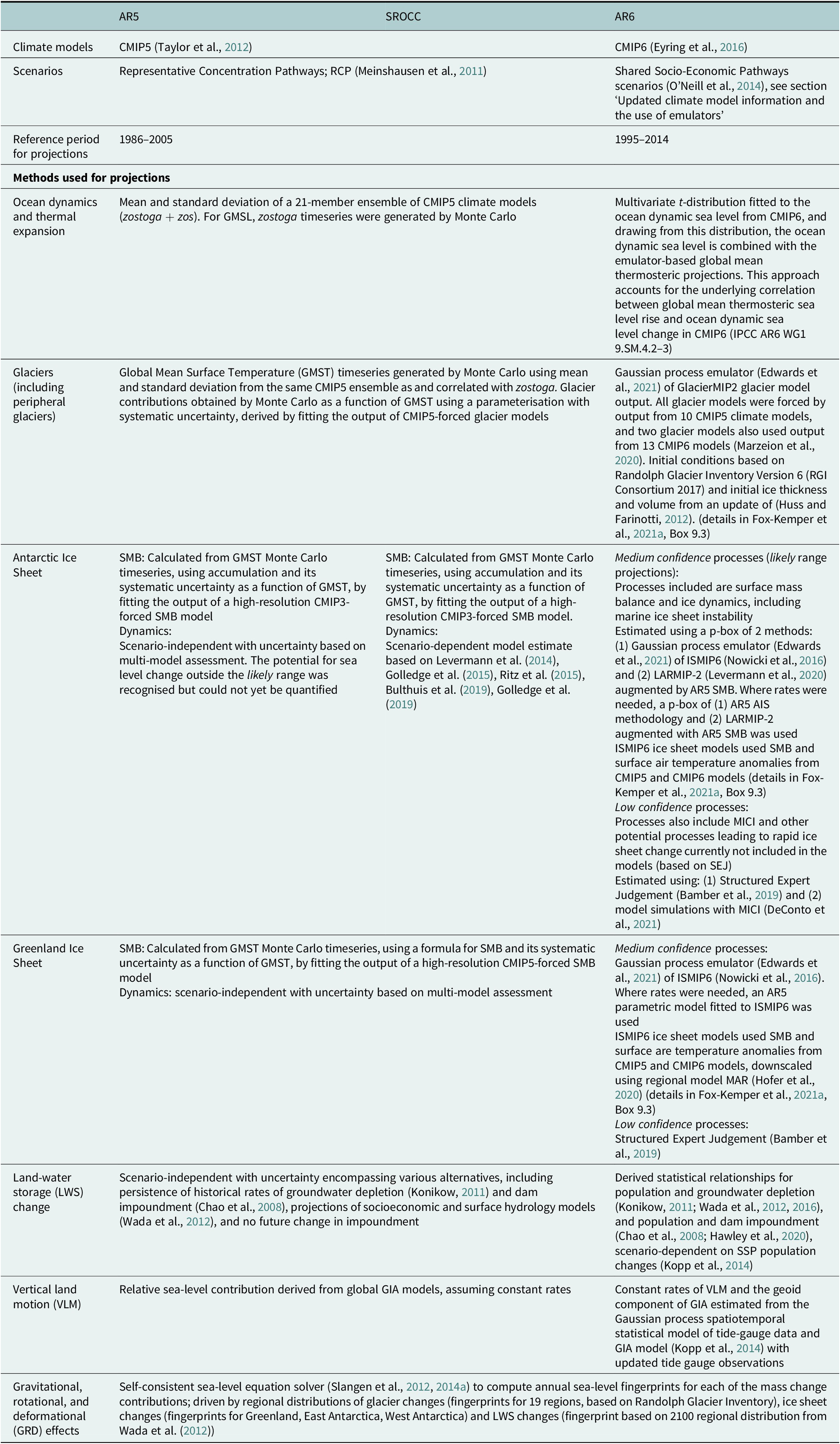
Note. This is an adapted version of Table 9.7 in Fox-Kemper et al. (Reference Fox-Kemper, Hewitt, Xiao, Aðalgeirsdóttir, Drijfhout, Edwards, Golledge, Hemer, Kopp, Krinner, Mix, Notz, Nowicki, Nurhati, Ruiz, Sallée, Slangen, Yu, Masson-Delmotte, Zhai, Pirani and Zhou2021a).
The methodologies of the projections in AR5, SROCC and AR6 are briefly summarised in Table 1; for more details, we refer to Chapter 13 of AR5 (Church et al., Reference Church, Clark, Cazenave, Gregory, Jevrejeva, Levermann, Merrifield, Milne, Nerem, Nunn, Payne, Pfeffer, Stammer, Unnikrishnan, Stocker, Qin, Plattner and Midgley2013a), Chapter 4 of SROCC (Oppenheimer et al., Reference Oppenheimer, Glavovic, Hinkel, van de Wal, Magnan, Abd-Elgawad, Cai, Cifuentes-Jara, DeConto, Ghosh, Hay, Isla, Marzeion, Meyssignac and Sebesvari2019) and Chapter 9 of AR6 (Fox-Kemper et al., Reference Fox-Kemper, Hewitt, Xiao, Aðalgeirsdóttir, Drijfhout, Edwards, Golledge, Hemer, Kopp, Krinner, Mix, Notz, Nowicki, Nurhati, Ruiz, Sallée, Slangen, Yu, Masson-Delmotte, Zhai, Pirani and Zhou2021a). We focus on three major elements of the projections that have changed: (1) the use of CMIP5 versus CMIP6 model output and consistency with the assessed ECS (section ‘Updated climate model information and the use of emulators’); (2) differences in the approaches to project the contributions to SLC (section ‘Differences in the projected contributions to SLC’); (3) the way the reports addressed potential outcomes outside the likely range (section ‘Sea-level projections outside the likely range’).
Updated climate model information and the use of emulators
The majority of the sea-level projections for the 21st century since AR5 have been based on CMIP5 climate model output (Taylor et al., Reference Taylor, Stouffer and Meehl2012), forced by Representative Concentration Pathways (RCP, Meinshausen et al., Reference Meinshausen, Smith, Calvin, Daniel, Kainuma, Lamarque, Matsumoto, Montzka, Raper, Riahi, Thomson, Velders and DPP2011), which are scenarios of future greenhouse gas concentrations and aerosol emissions. The projections in AR6 used information from CMIP6 climate models (Eyring et al., Reference Eyring, Bony, Meehl, Senior, Stevens, Stouffer and Taylor2016), which were forced by Shared Socioeconomic Pathways (SSP, O’Neill et al., Reference O’Neill, Kriegler, Riahi, Ebi, Hallegatte, Carter, Mathur and van Vuuren2014): scenarios of socio-economic development (including for instance population change, urbanisation and technological development) in combination with radiative forcing changes (GHG emissions and concentrations). These scenarios are noted as SSPx − y, where x denotes the SSP pathway (SSP1 sustainability, SSP2 middle-of-the-road, SSP3 regional rivalry, SSP4 inequality, SSP5 fossil fuel-intensive) and y the radiative concentration level in 2100 in W/m2. AR6 used five illustrative SSP scenarios: SSP1–1.9 (very low emissions), SSP1–2.6 (low emissions), SSP2–4.5 (intermediate emissions), SSP3–7.0 (high emissions) and SSP5–8.5 (very high emissions).
The ECS from the CMIP6 model ensemble has a higher average and a wider range compared to the CMIP5 model ensemble and compared to the AR6 assessment of ECS (Forster et al., Reference Forster, Storelvmo, Armour, Collins, Dufresne, Frame, Lunt, Mauritsen, Palmer, Watanabe, Wild, Zhang, Masson-Delmotte, Zhai, Pirani and Zhou2021). The consequences of this change in ECS distribution for projections of GMSL change were investigated by Hermans et al. (Reference Hermans, Gregory, Palmer, Ringer, Katsman and Slangen2021), who used CMIP6 data in combination with the AR5 methodology. They found that, while the projected change in GSAT median and range increased substantially from CMIP5 to CMIP6 (from 1.9 (1.1–2.6) K to 2.5 (1.6–3.5) K under SSP2-RCP4.5, see their Table S2 for additional scenarios), the upper end of the GMSL likely range projections at 2100 increased by only 3–7 cm across all scenarios (see their Figures 1 and 3), due to the delayed response of SLC to temperature changes. However, they also found an increase in the end-of-century GMSL rates of up to ~20%, suggesting that differences between CMIP5 and CMIP6-based GMSL projections could become substantially larger on longer time scales.
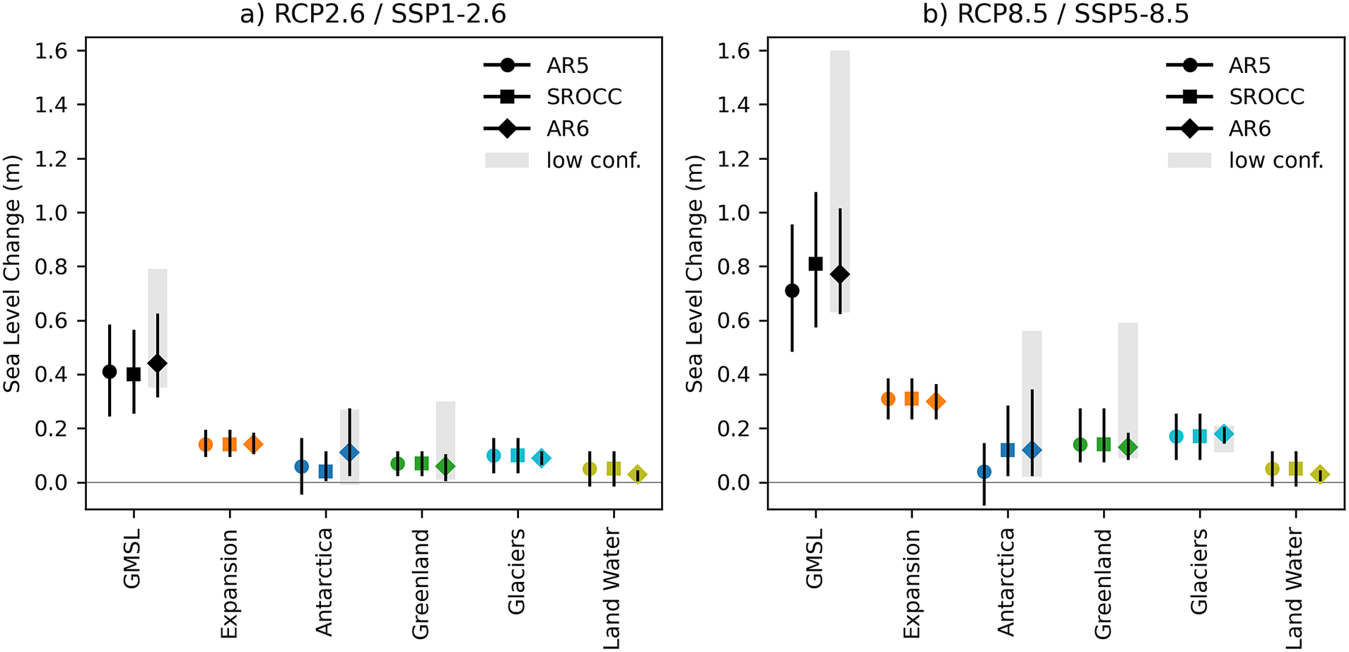
Figure 1. Comparison of 21st century projections of global mean SLC in AR5, SROCC and AR6. Total GMSL and individual contributions, between 1995 and 2014 and 2100 (m), median values and likely ranges of medium confidence projections, for (a) RCP2.6/SSP1–2.6 and (b) RCP8.5/SSP5–8.5. See also Table 9.8 in Fox-Kemper et al. (Reference Fox-Kemper, Hewitt, Xiao, Aðalgeirsdóttir, Drijfhout, Edwards, Golledge, Hemer, Kopp, Krinner, Mix, Notz, Nowicki, Nurhati, Ruiz, Sallée, Slangen, Yu, Masson-Delmotte, Zhai, Pirani and Zhou2021a) for comparative numbers of GMSL projections. AR6 low confidence projections for SSP1–2.6 and SSP5–8.5 in grey for Greenland, Antarctica and GMSL. Corrections for the differences in baseline period between AR5 (1986–2005) and AR6 (1995–2014) were done following IPCC AR6, Table 9.8.
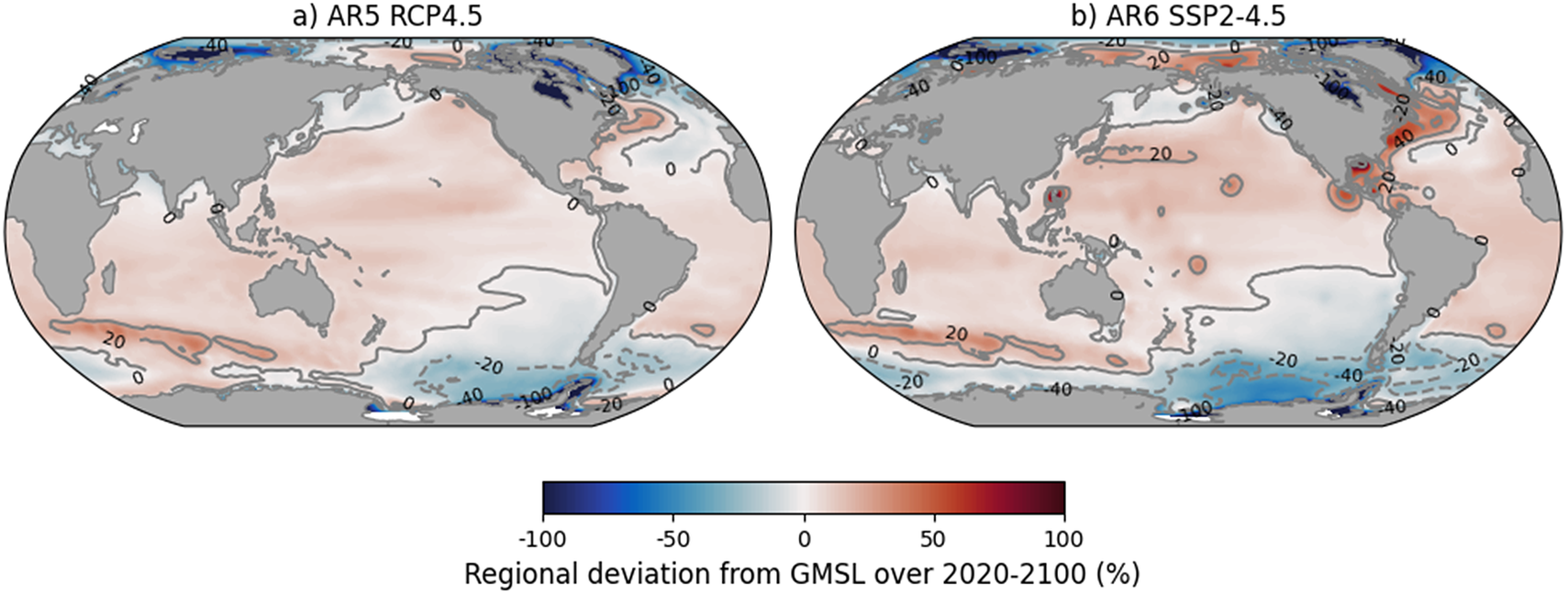
Figure 2. Comparison of regional relative sea-level change w.r.t. the global mean sea-level change in AR5 and AR6 (2020–2100) (%), based on median values, for (a) IPCC AR5 RCP4.5, global mean of 0.46 m and (b) IPCC AR6 SSP2–4.5, global mean of 0.51 m.
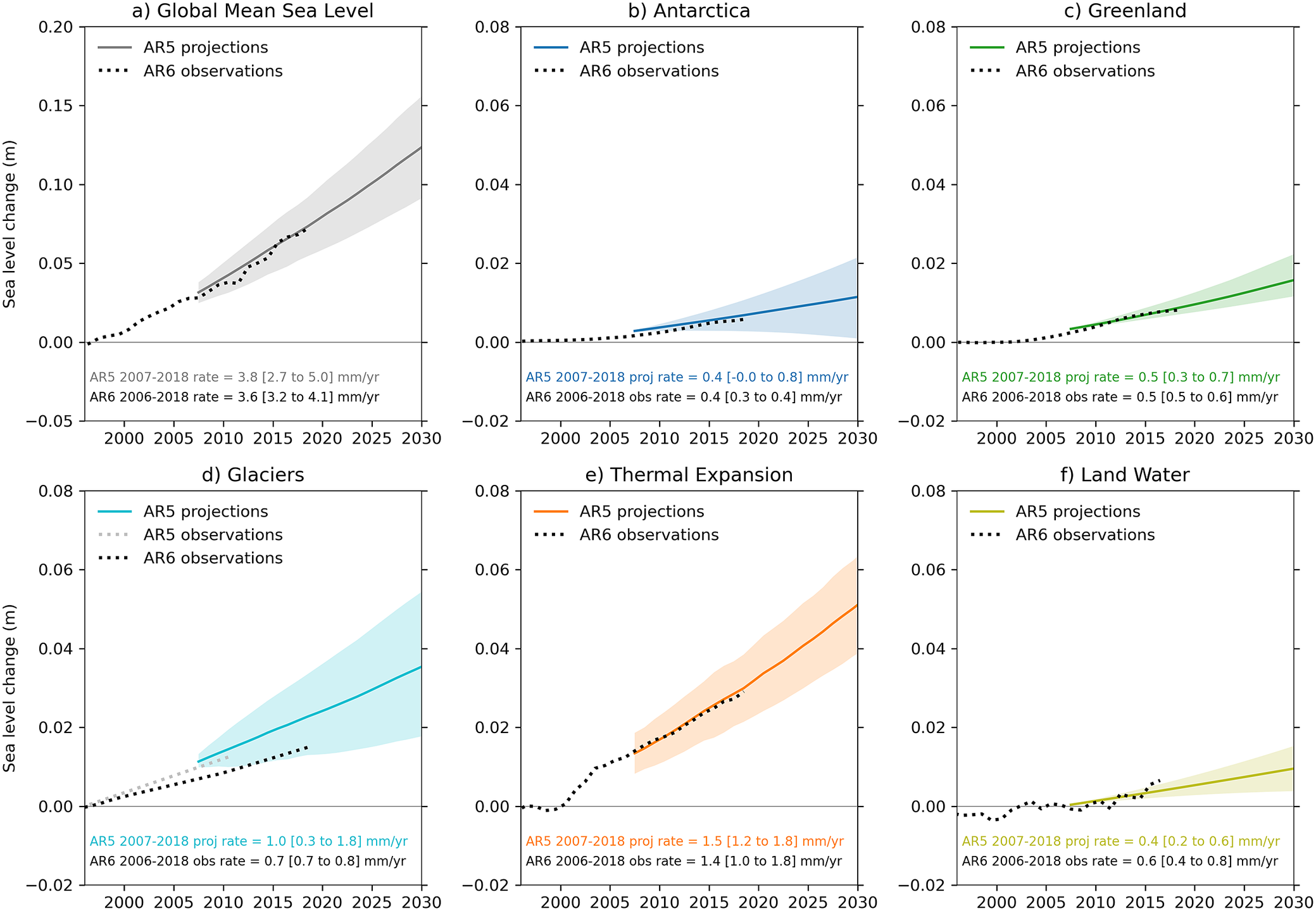
Figure 3. Comparison of observations (IPCC AR6, available up to 2018) and projections (IPCC AR5, available from 2007) of GMSL change. (a) Total GMSL and (b-f) individual contributions in (m) with respect to the period 1986–2005; all uncertainties recomputed to represent the likely range. Text in panels compares rates (mm/yr) of observations for 2006–2018 (Fox-Kemper et al., Reference Fox-Kemper, Hewitt, Xiao, Aðalgeirsdóttir, Drijfhout, Edwards, Golledge, Hemer, Kopp, Krinner, Mix, Notz, Nowicki, Nurhati, Ruiz, Sallée, Slangen, Yu, Masson-Delmotte, Zhai, Pirani and Zhou2021a, Table 9.5) to rates of projections for 2007–2018 (Church et al., Reference Church, Clark, Cazenave, Gregory, Jevrejeva, Levermann, Merrifield, Milne, Nerem, Nunn, Payne, Pfeffer, Stammer, Unnikrishnan, Stocker, Qin, Plattner and Midgley2013a); rates rounded to nearest 0.1 mm/yr; time periods used for rates differ by 1 year, allowing for traceability to the IPCC reports. Note that AR5 included the Greenland peripheral glaciers in the glacier contribution, whereas AR6 included it in the Greenland contribution; we have therefore subtracted a Greenland peripheral glacier estimate of 0.1 mm/yr from the AR6 Greenland observations in (c) and added it to the AR6 glacier observations in (d), both for the time series and the rates (Church et al., Reference Church, Clark, Cazenave, Gregory, Jevrejeva, Levermann, Merrifield, Milne, Nerem, Nunn, Payne, Pfeffer, Stammer, Unnikrishnan, Stocker, Qin, Plattner and Midgley2013a, Table 13.1; Fox-Kemper et al., Reference Fox-Kemper, Hewitt, Xiao, Aðalgeirsdóttir, Drijfhout, Edwards, Golledge, Hemer, Kopp, Krinner, Mix, Notz, Nowicki, Nurhati, Ruiz, Sallée, Slangen, Yu, Masson-Delmotte, Zhai, Pirani and Zhou2021b, Table 9.SM.2). The AR5 observed glacier change is added to (d) for reference (using the 1993–2010 linear rate from Table 13.1 of Church et al., Reference Church, Clark, Cazenave, Gregory, Jevrejeva, Levermann, Merrifield, Milne, Nerem, Nunn, Payne, Pfeffer, Stammer, Unnikrishnan, Stocker, Qin, Plattner and Midgley2013a).
One of the novel aspects of AR6 was the use of a physically-based emulator, which allowed for projections of 21st century GSAT and SLC that were consistent with the AR6 assessment of ECS (Forster et al., Reference Forster, Storelvmo, Armour, Collins, Dufresne, Frame, Lunt, Mauritsen, Palmer, Watanabe, Wild, Zhang, Masson-Delmotte, Zhai, Pirani and Zhou2021). The AR6 used a simple two-layer energy balance model (e.g., Geoffroy et al., Reference Geoffroy, Saint-Martin, Bellon, Voldoire, Olivié and Tytéca2013). Previous studies have used this two-layer model to successfully emulate CMIP5 model projections of GSAT and global mean thermosteric SLC to 2300 (Palmer et al., Reference Palmer, Harris and Gregory2018; Yuan and Kopp, Reference Yuan and Kopp2021). The AR6 emulator ensemble was constrained using four observational targets, including historical GSAT change and ocean heat uptake (Smith et al., Reference Smith, Nicholls, Armour, Collins, Forster, Meinshausen, Palmer, Watanabe, Masson-Delmotte, Zhai, Pirani and Zhou2021). The projected ocean heat uptake was translated to global mean thermosteric SLC using CMIP6-based estimates of expansion efficiency (Fox-Kemper et al., Reference Fox-Kemper, Hewitt, Xiao, Aðalgeirsdóttir, Drijfhout, Edwards, Golledge, Hemer, Kopp, Krinner, Mix, Notz, Nowicki, Nurhati, Ruiz, Sallée, Slangen, Yu, Masson-Delmotte, Zhai, Pirani and Zhou2021b). The GSAT changes were also used as input for the land-ice contributions to GMSL rise, which were generated with additional emulators applied to suites of coordinated community efforts for the ice sheet (LARMIP-2, Levermann et al., Reference Levermann, Winkelmann, Albrecht, Goelzer, Golledge, Greve, Huybrechts, Jordan, Leguy, Martin, Morlighem, Pattyn, Pollard, Quiquet, Rodehacke, Seroussi, Sutter, Zhang, Van Breedam, Calov, Deconto, Dumas, Garbe, Gudmundsson, Hoffman, Humbert, Kleiner, Lipscomb, Meinshausen, Ng, Nowicki, Perego, Price, Saito, Schlegel, Sun and Van De Wal2020; ISMIP6, Nowicki et al., Reference Nowicki, Payne, Larour, Seroussi, Goelzer, Lipscomb, Gregory, Abe-Ouchi and Shepherd2016) and glacier model (GlacierMIP2, Marzeion et al., Reference Marzeion, Hock, Anderson, Bliss, Champollion, Fujita, Huss, Immerzeel, Kraaijenbrink, Malles, Maussion, Radić, Rounce, Sakai, Shannon, van de Wal and Zekollari2020) simulations carried out for AR6.
Differences in the projected contributions to SLC
In AR5, the assessments of glacier and ice sheet contributions were based on a range of individual models and publications. The only difference in the SROCC projections with respect to AR5 was the reassessment of the Antarctic dynamics contribution, by replacing the AR5 Antarctic scenario-independent ice dynamic projections with scenario-dependent process-based model estimates (Levermann et al., Reference Levermann, Winkelmann, Nowicki, Fastook, Frieler, Greve, Hellmer, Martin, Meinshausen, Mengel, Payne, Pollard, Sato, Timmermann, Wang and Bindschadler2014; Golledge et al., Reference Golledge, Kowalewski, Naish, Levy, Fogwill and Gasson2015; Ritz et al., Reference Ritz, Edwards, Durand, Payne, Peyaud and Hindmarsh2015; Bulthuis et al., Reference Bulthuis, Arnst, Sun and Pattyn2019; Golledge et al., Reference Golledge, Keller, Gomez, Naughten, Bernales, Trusel and Edwards2019). This led to a decrease in 21st century GMSL change compared with AR5 for the RCP2.6 scenario, and an increase for the RCP8.5 scenario (medians and likely ranges; Figure 1a,b). However, the scenario-dependence in SROCC may have been amplified because two model estimates did not include accumulation changes (Levermann et al., Reference Levermann, Winkelmann, Nowicki, Fastook, Frieler, Greve, Hellmer, Martin, Meinshausen, Mengel, Payne, Pollard, Sato, Timmermann, Wang and Bindschadler2014; Ritz et al., Reference Ritz, Edwards, Durand, Payne, Peyaud and Hindmarsh2015), which are projected to increase with warming and partially counteract dynamic losses (Fox-Kemper et al., Reference Fox-Kemper, Hewitt, Xiao, Aðalgeirsdóttir, Drijfhout, Edwards, Golledge, Hemer, Kopp, Krinner, Mix, Notz, Nowicki, Nurhati, Ruiz, Sallée, Slangen, Yu, Masson-Delmotte, Zhai, Pirani and Zhou2021a).
For the AR6 projections, statistical emulators were applied to the ISMIP6 and GlacierMIP2 outputs, using the Gaussian process model described in Edwards et al. (Reference Edwards, Nowicki, Marzeion, Hock, Goelzer, Seroussi, Jourdain, Slater, Turner, Smith, McKenna, Simon, Abe-Ouchi, Gregory, Larour, Lipscomb, Payne, Shepherd, Agosta, Alexander, Albrecht, Anderson, Asay-Davis, Aschwanden, Barthel, Bliss, Calov, Chambers, Champollion, Choi, Cullather, Cuzzone, Dumas, Felikson, Fettweis, Fujita, Galton-Fenzi, Gladstone, Golledge, Greve, Hattermann, Hoffman, Humbert, Huss, Huybrechts, Immerzeel, Kleiner, Kraaijenbrink, Le clec’h, Lee, Leguy, Little, Lowry, Malles, Martin, Maussion, Morlighem, O’Neill, Nias, Pattyn, Pelle, Price, Quiquet, Radić, Reese, Rounce, Rückamp, Sakai, Shafer, Schlegel, Shannon, Smith, Straneo, Sun, Tarasov, Trusel, Van Breedam, van de Wal, van den Broeke, Winkelmann, Zekollari, Zhao, Zhang and Zwinger2021). For LARMIP-2, results for Antarctic ice sheet dynamics were emulated using an impulse-response function model following (Levermann et al., Reference Levermann, Winkelmann, Albrecht, Goelzer, Golledge, Greve, Huybrechts, Jordan, Leguy, Martin, Morlighem, Pattyn, Pollard, Quiquet, Rodehacke, Seroussi, Sutter, Zhang, Van Breedam, Calov, Deconto, Dumas, Garbe, Gudmundsson, Hoffman, Humbert, Kleiner, Lipscomb, Meinshausen, Ng, Nowicki, Perego, Price, Saito, Schlegel, Sun and Van De Wal2020), augmented by a parametric surface-mass balance model following AR5. There were several motivations for using these emulators: (1) to constrain the projections to the assessed ECS range, an approach that represents a marked change from previous IPCC reports; (2) to be able to make projections across all five illustrative SSP scenarios of AR6, as the ice sheet and glacier contributions were mostly based on CMIP5 RCP scenarios; and (3) to sample modelling uncertainties more thoroughly, estimating probability distributions for the contributions. The use of simple climate models and emulators is a trade-off between a more complete exploration of the uncertainties which can be done due to the computational speed of the emulators (compared to the full ice sheet and glacier models, which are limited by constraints of computing and person time), and the potential biases introduced by the necessary assumptions of a simpler model (Edwards et al., Reference Edwards, Nowicki, Marzeion, Hock, Goelzer, Seroussi, Jourdain, Slater, Turner, Smith, McKenna, Simon, Abe-Ouchi, Gregory, Larour, Lipscomb, Payne, Shepherd, Agosta, Alexander, Albrecht, Anderson, Asay-Davis, Aschwanden, Barthel, Bliss, Calov, Chambers, Champollion, Choi, Cullather, Cuzzone, Dumas, Felikson, Fettweis, Fujita, Galton-Fenzi, Gladstone, Golledge, Greve, Hattermann, Hoffman, Humbert, Huss, Huybrechts, Immerzeel, Kleiner, Kraaijenbrink, Le clec’h, Lee, Leguy, Little, Lowry, Malles, Martin, Maussion, Morlighem, O’Neill, Nias, Pattyn, Pelle, Price, Quiquet, Radić, Reese, Rounce, Rückamp, Sakai, Shafer, Schlegel, Shannon, Smith, Straneo, Sun, Tarasov, Trusel, Van Breedam, van de Wal, van den Broeke, Winkelmann, Zekollari, Zhao, Zhang and Zwinger2021). The Gaussian process emulator performed well for the cumulative change in time, but did not account for temporal correlation, so the rates could not be estimated from the emulator. As a consequence, in contexts where rates were needed, AR6 used simpler parametric emulators, based on approaches used in AR5.
A comparison of the GMSL projections to 2100 in the different reports reveals a number of differences (Figure 1a,b). In the land ice contributions, we see a narrowing of the likely ranges for glaciers (under both scenarios) and the Greenland ice sheet (under SSP5–8.5), and a widening of the Antarctic ice sheet likely range. The latter is wider as it is based on a p-box bounding distribution functions from the ISMIP6 emulator and LARMIP-2 (Table 1), where the presented likely range spans from the lowest 17th to the highest 83rd percentile of the considered methods. The ECS-constrained temperature projections in AR6 (section ‘Updated climate model information and the use of emulators’) used as input to the land ice emulators show a marked reduction in the width of the likely range at 2100 (~0.7 K for SSP1–2.6; ~1.9 K for SSP5–8.5) compared with the 21 CMIP5 models used as the basis of the AR5 sea-level projections (~1.6 K for RCP2.6; ~2.8 K for RCP8.5), which could also be one of the reasons for the reduced width of the glacier and Greenland likely ranges. The glacier range may also be slightly underestimated because each region is emulated independently, which means the projections do not account for covariances in the regional uncertainties apart from those associates with a common dependence on temperature (Marzeion et al., Reference Marzeion, Hock, Anderson, Bliss, Champollion, Fujita, Huss, Immerzeel, Kraaijenbrink, Malles, Maussion, Radić, Rounce, Sakai, Shannon, van de Wal and Zekollari2020; Fox-Kemper et al., Reference Fox-Kemper, Hewitt, Xiao, Aðalgeirsdóttir, Drijfhout, Edwards, Golledge, Hemer, Kopp, Krinner, Mix, Notz, Nowicki, Nurhati, Ruiz, Sallée, Slangen, Yu, Masson-Delmotte, Zhai, Pirani and Zhou2021a, Section 9.5). However, the AR5 glacier and Greenland uncertainties were open-ended (≥ 66% ranges) and essentially estimated with expert judgement, at a time of far less information from – and confidence in – these process-based models, so the narrowing range is also consistent with an improving evidence base. The land-water storage contribution is reduced in AR6 compared with AR5 due to the use of a different methodology which now links land-water storage changes to global population under SSP scenarios (Kopp et al., Reference Kopp, Horton, Little, Mitrovica, Oppenheimer, Rasmussen, Strauss and Tebaldi2014), in combination with a larger negative reservoir impoundment contribution from Hawley et al. (Reference Hawley, Hay, Mitrovica and Kopp2020).
AR5 used different methodologies for estimating the uncertainties in GMSL (Figure 1a,b) and regional SLC (Church et al., Reference Church, Clark, Cazenave, Gregory, Jevrejeva, Levermann, Merrifield, Milne, Nerem, Nunn, Payne, Pfeffer, Stammer, Unnikrishnan, Stocker, Qin, Plattner and Midgley2013b). In contrast, the AR6 GMSL (Figure 1a,b) and regional projected uncertainties are combined in the same way, with the different contributions all treated as conditionally independent given GSAT, which is an input for the emulator (Fox-Kemper et al., Reference Fox-Kemper, Hewitt, Xiao, Aðalgeirsdóttir, Drijfhout, Edwards, Golledge, Hemer, Kopp, Krinner, Mix, Notz, Nowicki, Nurhati, Ruiz, Sallée, Slangen, Yu, Masson-Delmotte, Zhai, Pirani and Zhou2021b). The total projected GMSL for SSP1–2.6 has increased in AR6 compared with RCP2.6 projections in AR5 and SROCC, with a similar likely range (Figure 1a), but with different relative contributions of each component. For SSP5–8.5, the AR6 GMSL projections are 4 cm lower than RCP8.5 in SROCC but 6 cm higher than RCP8.5 in AR5 (Figure 1b), due to differences in the model estimates included (from AR5 to SROCC) and in both models used and the methods used to combine the models (from SROCC to AR6) of the projected Antarctic contribution.
The regional projections (Figure 2) show that SLC is spatially highly variable, due to a combination of ocean dynamic changes, gravitational, rotational and deformation (GRD) effects in response to present-day mass changes, and long-term Glacial Isostatic Adjustment (GIA). There is an overall agreement in the patterns between AR5 and AR6. Some differences arise from the vertical land motion (VLM) contribution, which included only GIA in AR5 and also other VLM contributions, such as tectonics, compaction or anthropogenic subsidence, in AR6: compare for instance the larger ratios along the US East Coast ( Figure 2b) to the VLM contribution in Figure 9.26 from Fox-Kemper et al. (Reference Fox-Kemper, Hewitt, Xiao, Aðalgeirsdóttir, Drijfhout, Edwards, Golledge, Hemer, Kopp, Krinner, Mix, Notz, Nowicki, Nurhati, Ruiz, Sallée, Slangen, Yu, Masson-Delmotte, Zhai, Pirani and Zhou2021a). The increased contribution from Antarctica compared to AR5, in combination with the ocean dynamics contribution, leads to a more widespread below-average SLC in the Antarctic Circumpolar Current region.
Sea-level projections outside the likely range
One of the key uncertainties in sea-level projections is the dynamic contribution of the ice sheets (i.e., processes related to the flow of the ice). AR5 assessed the likely dynamical contribution of the Antarctic Ice Sheet by 2100 at −2 to 18.5 cm, but also noted that ‘Based on current understanding, only the collapse of marine-based sectors of the Antarctic ice sheet, if initiated, could cause global mean sea level to rise substantially above the likely range during the 21st century. There is medium confidence that this additional contribution would not exceed several tenths of a metre of sea level rise during the 21st century’. An ice sheet estimate based on SEJ was available at the time of AR5 but this could not be supported by other lines of evidence (Church et al., Reference Church, Clark, Cazenave, Gregory, Jevrejeva, Levermann, Merrifield, Milne, Nerem, Nunn, Payne, Pfeffer, Stammer, Unnikrishnan, Stocker, Qin, Plattner and Midgley2013a). Including the SEJ estimates would have led to an assessment that could not be transparently linked to physical evidence, as the reasoning of the experts involved in the SEJ exercise is undocumented, and it was decided not to use it for the AR5 assessment.
After AR5, following for instance Sutton (Reference Sutton2019), low probability estimates were increasingly used in the context of risk assessment and to discuss less likely outcomes for risk-averse users (e.g., Le Cozannet et al., Reference Le Cozannet, Nicholls, Hinkel, Sweet, McInnes, Van de Wal, Slangen, Lowe and White2017b; Hinkel et al., Reference Hinkel, Church, Gregory, Gregory, Lambert, McInnes, Nicholls, Church, van der Pol and van de Wal2019; Nicholls et al., Reference Nicholls, Hanson, Lowe, Slangen, Wahl, Hinkel and Long2021). SROCC argued that stakeholders with a low risk tolerance might use the SEJ numbers (e.g., their Figure 4.2). Model results including marine ice cliff instability (MICI, Deconto and Pollard, Reference Deconto and Pollard2016) were not used in the main projections of SROCC because the too high surface melt rates led to an uncertain timing and magnitude in the simulated ice loss. In AR6, a set of low confidence projections was presented (shown in grey in Figure 1a,b) which build on the medium confidence projections. These projections include additional contributions for the ice sheets, estimated using a p-box approach (e.g., Le Cozannet et al., Reference Le Cozannet, Manceau and Rohmer2017a), considering SEJ (Bamber et al., Reference Bamber, Oppenheimer, Kopp, Aspinall and Cooke2019) together with an improved model-based estimate for Antarctica which included MICI (DeConto et al., Reference DeConto, Pollard, Alley, Velicogna, Gasson, Gomez, Sadai, Condron, Gilford, Ashe, Kopp, Li and Dutton2021). It is important to note that the low confidence ranges represent the breadth of literature estimates available at the time, but that they are not incorporated in the assessed likely ranges.
The AR6 low confidence projections suggest that by 2100, under SSP1–2.6 ( Figure 1a), there is a potential Greenland contribution outside the likely range, based on SEJ. For Antarctica, the medium confidence SSP1–2.6 projections already include a wide range of values, so the impact of SEJ and MICI estimates in the lowconfidence projections is less distinct. Under SSP5–8.5 (Figure 1b), the upper values of the AR6 low confidence projections for both ice sheets are considerably larger than the corresponding medium confidence estimates. This reflects the deep uncertainty in the literature on the Antarctic contribution (see also Box 9.4 in Fox-Kemper et al., Reference Fox-Kemper, Hewitt, Xiao, Aðalgeirsdóttir, Drijfhout, Edwards, Golledge, Hemer, Kopp, Krinner, Mix, Notz, Nowicki, Nurhati, Ruiz, Sallée, Slangen, Yu, Masson-Delmotte, Zhai, Pirani and Zhou2021a). What is needed to reduce this deep uncertainty is primarily a better understanding of the physical processes. This will lead to more physically-based model projections with larger ensembles, which will allow for a better exploration of the uncertainties.
Comparison of the AR5 model simulations with observations
In the previous section, we discussed ‘how we got here’: the developments that led to the most recent IPCC projections. However, it is also relevant to see ‘where we are’, by comparing the observed sea-level change against sea-level projections for their overlapping period. We evaluate the assessed likely ranges of the AR5 projections (from 2007 onwards, Church et al., Reference Church, Clark, Cazenave, Gregory, Jevrejeva, Levermann, Merrifield, Milne, Nerem, Nunn, Payne, Pfeffer, Stammer, Unnikrishnan, Stocker, Qin, Plattner and Midgley2013a) against the assessed observational time series from AR6 (up to 2018, Fox-Kemper et al., Reference Fox-Kemper, Hewitt, Xiao, Aðalgeirsdóttir, Drijfhout, Edwards, Golledge, Hemer, Kopp, Krinner, Mix, Notz, Nowicki, Nurhati, Ruiz, Sallée, Slangen, Yu, Masson-Delmotte, Zhai, Pirani and Zhou2021a, Table 9.5), both for the total GMSL and the individual contributions (Figure 3).
For GMSL, Antarctica, Greenland and thermal expansion, the observational timeseries are close to the centre of the projections and the estimated rates of change are highly consistent (Figure 3a,b,c,e). The observed glacier timeseries in AR6 is at the lower end of the projections, even though the observed rates entirely fall within the likely range of the projected rates (Figure 3d). It is worth noting that the AR5 included glaciers peripheral to the Greenland Ice Sheet in the glacier projections (their Table 13.5), which according to the observations in their Table 13.1 adds a contribution in the order of 0.1 mm/yr. In AR6, this was included in the Greenland contribution. To facilitate the comparison, we have included the observed Greenland peripheral glacier estimate in Figure 3d (Glaciers) and subtracted it from the observations in Figure 3c (Greenland), based on linear rates presented in Church et al., Reference Church, Clark, Cazenave, Gregory, Jevrejeva, Levermann, Merrifield, Milne, Nerem, Nunn, Payne, Pfeffer, Stammer, Unnikrishnan, Stocker, Qin, Plattner and Midgley2013a and Fox-Kemper et al., Reference Fox-Kemper, Hewitt, Xiao, Aðalgeirsdóttir, Drijfhout, Edwards, Golledge, Hemer, Kopp, Krinner, Mix, Notz, Nowicki, Nurhati, Ruiz, Sallée, Slangen, Yu, Masson-Delmotte, Zhai, Pirani and Zhou2021a. In addition, the glacier contributions since AR5 suggest a smaller glacier contribution, both in observations and projections (for the observations: grey dashed line in Figure 3d based on Church et al., Reference Church, Clark, Cazenave, Gregory, Jevrejeva, Levermann, Merrifield, Milne, Nerem, Nunn, Payne, Pfeffer, Stammer, Unnikrishnan, Stocker, Qin, Plattner and Midgley2013a, Table 13.1 shows a higher rate than AR6, for the projections: Marzeion et al., Reference Marzeion, Leclercq, Cogley and Jarosch2015). The observed rate of land-water change is larger than the projected central value, but the observed time series, despite its interannual variability, mostly falls within the projected likely range. The observed rate of change is at the upper bound of the likely range projections (Figure 3f).
Wang et al. (Reference Wang, Church, Zhang and Chen2021a) also evaluated GMSL and regional projections from AR5 and SROCC against different tide gauge and altimetry time series for the period 2007–2018. They found that the GMSL trends for 2007–2018 from AR5 projections are almost identical to observed trends and well within the 90% confidence interval. They also showed significant local differences between observations and models, which could be improved with better VLM estimates and minimisation of the internal variability.
A study by Lyu et al. (Reference Lyu, Zhang and Church2021) focused on ocean warming, with the purpose of constraining projections. They compared the observations of ocean temperature by the Argo array (2005–2019) with model simulations from the CMIP5 and CMIP6 databases. They found that (1) the range of CMIP6 has shifted upwards compared with CMIP5; (2) there is a high correlation between observations and models over the Argo period; (3) the emergent constraint indicates that the larger trend of thermosteric SLC in the CMIP6 archive needs to be taken with caution. This supports the AR6 approach, where an emulator was used to constrain the thermosteric SLC of CMIP6 models with the assessed ECS range (section ‘Updated climate model information and the use of emulators’), leading to thermosteric SLC projections similar to AR5 and the constrained Lyu et al. (Reference Lyu, Zhang and Church2021) projections.
Moving towards local information
AR5 was the first IPCC assessment report to show regional sea-level projections in addition to GMSL projections, by including the effects of changes in ocean density and circulation, GIA and GRD effects (Table 1). SROCC built on AR5 but explored regional changes in sea-level extremes in more depth. In AR6 as a whole, even stronger emphasis was put on regional climate changes and on using regional information for impacts and risk assessment, in particular in Chapter 10 (Doblas-Reyes et al., Reference Doblas-Reyes, Sörensson, Almazroui, Dosio, Gutowski, Haarsma, Hamdi, Hewitson, Kwon, Lamptey, Maraun, Stephenson, Takayabu, Terray, Turner, Zuo, Masson-Delmotte, Zhai, Pirani and Zhou2021), Chapter 12 (Ranasinghe et al., Reference Ranasinghe, Ruane, Vautard, Arnell, Coppola, Cruz, Dessai, Islam, Rahimi, Ruiz, Sillmann, Sylla, Tebaldi, Wang, Zaaboul, Masson-Delmotte, Zhai, Pirani and Zhou2021) and the Interactive Atlas (Gutiérrez et al., Reference Gutiérrez, Jones, Narisma, Alves, Amjad, Gorodetskaya, Grose, Klutse, Krakovska, Li, Martínez-Castro, Mearns, Mernild, Ngo-Duc, van den Hurk, Yoon, Masson-Delmotte, Zhai, Pirani and Zhou2021). The IPCC authors and the IPCC Technical Support Unit also collaborated with NASA to develop the NASA/IPCC Sea Level Projection Tool (https://sealevel.nasa.gov/ipcc-ar6-sea-level-projection-tool) to provide easy access to global and regional projections. As the need for more detailed sea-level information is becoming increasingly evident (e.g., Le Cozannet et al., Reference Le Cozannet, Nicholls, Hinkel, Sweet, McInnes, Van de Wal, Slangen, Lowe and White2017b; Hinkel et al., Reference Hinkel, Church, Gregory, Gregory, Lambert, McInnes, Nicholls, Church, van der Pol and van de Wal2019; Nicholls et al., Reference Nicholls, Hanson, Lowe, Slangen, Wahl, Hinkel and Long2021; Durand et al., Reference Durand, van den Broeke, Le Cozannet, Edwards, Holland, Jourdain, Marzeion, Mottram, Nicholls, Pattyn, Paul, Slangen, Winkelmann, Burgard, van Calcar, Barré, Bataille and Chapuis2022), we discuss a couple of potential future research avenues which may help to further improve sea-level projections on a regional to local scale.
High-resolution ocean modelling
Ocean dynamic SLC is a major driver of spatial sea-level variability, which is typically derived from CMIP5 and CMIP6 GCM simulations. However, the extent to which GCMs can provide local information is limited because of their relatively low atmosphere and ocean grid resolutions, which are constrained by computational costs. The typical ocean grid resolution of CMIP5 models is approximately 1° by 1° (~100 km). Although the ocean components of some CMIP6 models operate at a 0.25° resolution, the resolution of most CMIP6 models has not increased much relative to CMIP5, and the CMIP5 and CMIP6 simulations of ocean dynamic SLC show similar features (Lyu et al., Reference Lyu, Zhang and Church2020). These relatively coarse resolutions may lead to misrepresentations of ocean dynamic SLC, particularly in coastal regions in which small-scale and tidal processes and bathymetric features are important. Increasing the resolution of the GCMs requires significant additional computational resources as well as more explicit modelling of high-resolution processes that are currently parameterized.
As an alternative, GCMs can be dynamically downscaled using high-resolution atmosphere or ocean models. Emerging research demonstrates the value of dynamical downscaling for SLC simulations in coastal regions such as the Northwestern European Shelf (Figure 4; Hermans et al., Reference Hermans, Tinker, Palmer, Katsman, Vermeersen and Slangen2020; Chaigneau et al., Reference Chaigneau, Reffray, Voldoire and Melet2022; Hermans et al., Reference Hermans, Katsman, Camargo, Garner, Kopp and Slangen2022), the Southern Ocean (Zhang et al., Reference Zhang, Church, Monselesan and McInnes2017), the Mediterranean Sea (Sannino et al., Reference Sannino, Carillo, Iacono, Napolitano, Palma, Pisacane and Struglia2022), the marginal seas in the Northwest Pacific Ocean (Liu et al., Reference Liu, Minobe, Sasaki and Terada2016; Kim et al., Reference Kim, Kim, Jeong, Lee, Byun and Cho2021), the marginal seas near China (Jin et al., Reference Jin, Zhang, Church and Bao2021) and the Brazilian continental shelf (Toste et al., Reference Toste, Assad and Landau2018), on both annual and sub-annual timescales. Additionally, dynamical downscaling can offer a framework in which local changes in tides, surges and waves can be resolved in conjunction with time-mean SLC and incorporated into sea-level projections (Kim et al., Reference Kim, Kim, Jeong, Lee, Byun and Cho2021; Chaigneau et al., Reference Chaigneau, Reffray, Voldoire and Melet2022), as it allows for modelling changes at higher temporal frequencies. Dynamical downscaling requires GCM output as boundary conditions, which means that the regional solutions due to the explicit modelling of higher resolution processes should always be considered in the context of the GCM model that is driving the regional model. For instance, for the South China Sea, Jin et al. (Reference Jin, Zhang, Church and Bao2021) found that ‘the downscaled results driven by ensemble mean forcings are almost identical to the ensemble average results from individually downscaled cases’. However, more extensive analysis of the uncertainties associated with dynamical downscaling remains to be done. As a result, the dynamical downscaling of ocean simulations has not yet been systematically applied in the context of regional and local sea-level projections.
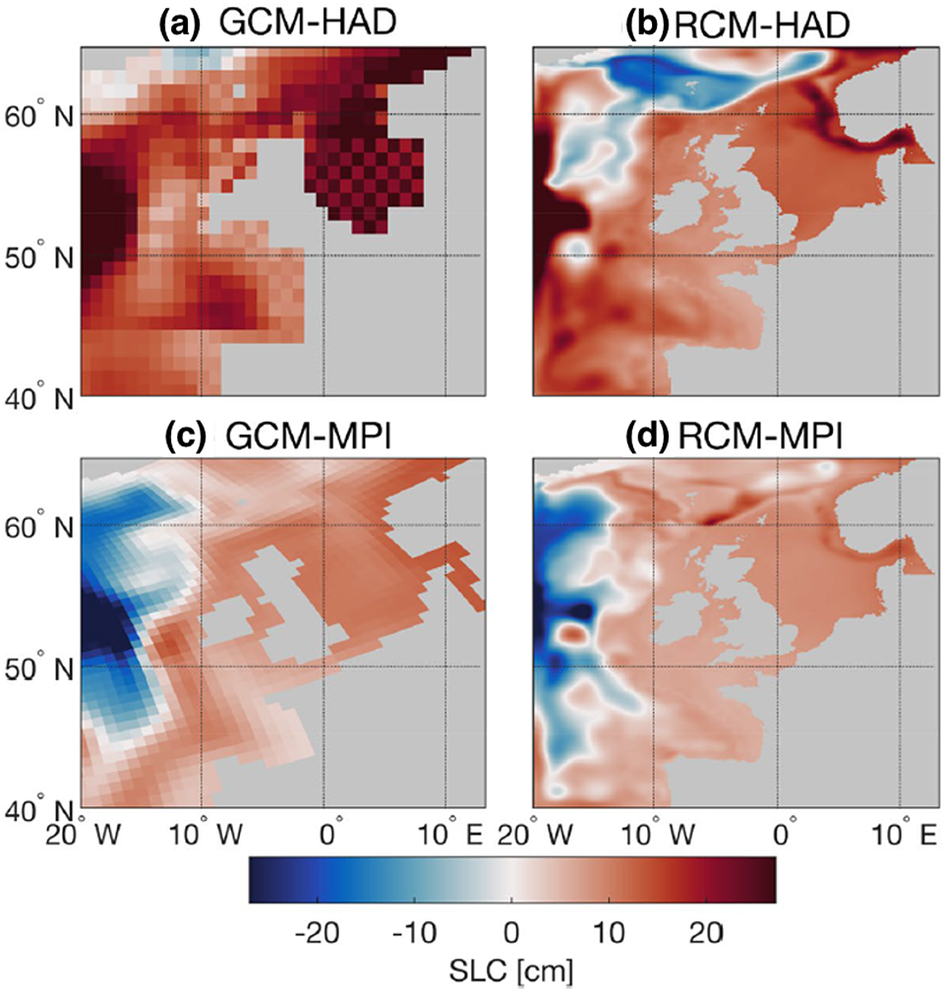
Figure 4. Ocean dynamic SLC northwest of Europe, as simulated by (a) the CMIP5 GCM HadGEM2-ES and (b) dynamically downscaled using regional ocean model NEMO-AMM7, and by (c) the CMIP5 GCM MPI-ESM-LR and (d) dynamically downscaled, for the scenario RCP8.5 (2074–2099 minus 1980–2005). Figure adapted from Hermans et al. (Reference Hermans, Tinker, Palmer, Katsman, Vermeersen and Slangen2020).
Vertical land motion
In addition to the ocean and ice contributions, relative SLC is affected by VLM (Table 1), which may amplify or even dominate the SLC experienced at coastal locations. AR5 and SROCC used GIA models to estimate the VLM contribution to SLC, whereas AR6 based its VLM estimate on the geological background rate at tide gauge stations, derived using the Gaussian Process Model from (Kopp et al., Reference Kopp, Horton, Little, Mitrovica, Oppenheimer, Rasmussen, Strauss and Tebaldi2014; Table 1). Neither method provides a satisfactory answer, given that the former excludes non-GIA VLM contributions, and the latter requires assumptions regarding the spatio-temporal extrapolation of the tide-gauge derived background rates to areas without tide gauge information by using a GIA model as a prior. AR6, therefore, stated that ‘there is low to medium confidence in the GIA and VLM projections employed in this Report. In many regions, higher-fidelity projections would require more detailed regional analysis’.
Work published after the IPCC AR6 literature deadline has provided new observation-based estimates of VLM for 99 coastal cities based on InSAR observations (Wu et al., Reference Wu, Wei and D’Hondt2022) and along the world’s coastlines using GNSS data (Oelsmann et al., Reference Oelsmann, Passaro, Dettmering, Schwatke, Sánchez and Seitz2021). However, even with better observational estimates, significant assumptions are required when extrapolating these into the future. Both AR5 and AR6 assume VLM rates remain constant over time, an assumption that is wrong in regions that are tectonically active (where VLM will be nonlinear and stochastic) or where VLM occurs in response to groundwater and gas extractions (which is strongly dependent on societal choices). A potential solution is to use expanded geological reconstructions of paleo sea level on millennial time scales to constrain long-term average trends (Horton et al., Reference Horton, Shennan, Bradley, Cahill, Kirwan, Kopp and Shaw2018b).
Conclusions and future perspectives
In this overview, we have discussed several aspects of sea-level projections: recent developments in the projections, how they compare against observations, and potential future research directions: ‘how we got here’ (section ‘Key advances in sea-level projections up to IPCC AR6’), ‘where we are’ (section ‘Comparison of the AR5 model simulations with observations’) and ‘where we’re going’ (section ‘Moving towards local information’).
Key differences between AR5, SROCC and AR6 include the use of new climate model information (CMIP6) and the use of emulators to constrain the projections to the AR6 assessment of Equilibrium Climate Sensitivity (section ‘Updated climate model information and the use of emulators’), new information for the different projected contributions to sea-level change (section ‘Differences in the projected contributions to SLC’), and the treatment of projections outside the likely range (section ‘Sea-level projections outside the likely range’).
The likely range projections of GMSL and regional SLC at 2100 show relatively modest changes from AR5 to SROCC and AR6, given approximately equivalent climate change scenarios (sections ‘Updated climate model information and the use of emulators’ and ‘Differences in the projected contributions to SLC’): under RCP2.6/SSP1–2.6 from 0.25–0.58 m (AR5) to 0.33–0.62 m (AR6); under RCP8.5/SSP5–8.5 from 0.49–0.95 m (AR5) to 0.63–1.01 m (AR6). Substantial reductions in the uncertainty of the Greenland and glacier contributions to GMSL at 2100 under SSP5–8.5 for AR6 are counterbalanced by an increase in the Antarctic uncertainty, which leads to relatively small changes in overall uncertainty at 2100 between AR5 and AR6.
In AR6, the explicit inclusion of low confidence projections highlighted the deep uncertainty associated with the dynamical ice sheet contribution (section ‘Sea-level projections outside the likely range’), which was communicated through the use of ‘low-likelihood high-impact’ storylines (IPCC, Reference Masson-Delmotte, Zhai, Pirani, Connors, Péan, Berger, Caud, Chen, Goldfarb, Gomis, Huang, Leitzell, Lonnoy, JBR, Maycock, Waterfield, Yelekçi, Yu and Zhou2021; Fox-Kemper et al., Reference Fox-Kemper, Hewitt, Xiao, Aðalgeirsdóttir, Drijfhout, Edwards, Golledge, Hemer, Kopp, Krinner, Mix, Notz, Nowicki, Nurhati, Ruiz, Sallée, Slangen, Yu, Masson-Delmotte, Zhai, Pirani and Zhou2021a). Regional SLC projections based on the low confidence projections were also provided by AR6, but we highlight that more work is needed on understanding and physical modelling of the ice sheet contributions, and on the potential for different regional estimates associated with the partitioning of Greenland and Antarctic ice mass loss.
Our comparison of AR5 projections with observations for the period 2007–2018 shows that the rates of change agree within uncertainties for GMSL and for individual contributions (section ‘Comparison of the AR5 model simulations with observations’), which is in line with previous studies focusing on total sea-level change (Wang et al., Reference Wang, Church, Zhang and Chen2021a) and the ocean heat uptake contribution (Lyu et al., Reference Lyu, Zhang and Church2021). Monitoring the projections against observed changes is important as it can help to constrain future projections.
In terms of future developments of sea-level projections (section ‘Moving towards local information’), we highlight the need for dynamical ocean downscaling to represent processes missing in GCMs, such as tidal effects and local currents in shelf sea regions, to better estimate future ocean dynamic SLC. This would also improve simulations of key small-scale processes at the ocean-ice interface that affect the climatic drivers of ice sheets and therefore projections of their future evolution. It would also lead to a better quantification of the effects on mean SLC on, for example, tidal characteristics and wave propagations to understand the potential compounding effects on future coastal flood hazards. A second aspect that is relevant to relative sea-level projections, in particular in low-lying delta regions, is the need for improved VLM observational estimates and projections. This will particularly impact coastal SLC projections, as flood risks depend on (and in some parts of the world are dominated by) the movement of the land in addition to the changes in water level.
In this paper, we have focused on sea-level projections up to 2100. However, it is important to note that sea-level change does not stop in 2100. Currently, projections beyond 2100 are typically based on different methods compared with the projections up to 2100, due to a lack of model simulations and literature. For instance, in AR6 the time series were extended to 2150 assuming constant ice sheet rates post 2100 and the Gaussian process emulators were substituted with parametric fits. Unfortunately, the use of different methods tends to lead to discontinuities in the time series. To fill this gap, we need better understanding and process modelling of the different components, such that consistent methods can be used to generate long-term projections for the next IPCC assessment report and beyond. This will allow investigations of for instance the sea-level response to surface warming overshoot scenarios, or the inclusion of tipping points in sea-level projections (e.g., Lenton et al., Reference Lenton, Rockström, Gaffney, Rahmstorf, Richardson, Steffen and Schellnhuber2019). These are only some of the many potential research avenues associated with long-term sea-level projections, all of which are important to investigate given the long-lasting commitment and widespread consequences of future sea-level rise.
Open peer review
To view the open peer review materials for this article, please visit http://doi.org/10.1017/cft.2022.8.
Data availability statement
All data used for the figures are publicly available from the following sources: IPCC AR5 sea-level projections: https://www.cen.uni-hamburg.de/en/icdc/data/ocean/ar5-slr.html; IPCC SROCC sea-level projections: https://ipcc-temp.s3.eu-central-1.amazonaws.com/SROCC_Ch04-SM_DataFiles.zip; IPCC AR6 sea-level projections: https://doi.org/10.5281/zenodo.5914709, with supplemental data sets documented at https://github.com/Rutgers-ESSP/IPCC-AR6-Sea-Level-Projections and IPCC AR6 sea-level observations: https://github.com/BrodiePearson/IPCC_AR6_Chapter9_Figures (Cross-Chapter Box 9.1 data).
Acknowledgements
We acknowledge the World Climate Research Programme, which, through its Working Group on Coupled Modelling, coordinated and promoted CMIP and ISMIP6. We thank the climate modelling groups for producing and making available their model output, the Earth System Grid Federation (ESGF) for archiving the data and providing access and the multiple funding agencies that support CMIP and ESGF.
Author contributions
M.D.P. conceived the study. A.B.A.S. led the writing of the manuscript. M.D.P., A.B.A.S., C.M.L.C. and T.H.J.H. produced figures. All authors contributed to writing the text and revising the manuscript.
Financial support
A.B.A.S., T.L.E., V.M.S. and T.H.J.H. were supported by PROTECT. This project has received funding from the European Union’s Horizon 2020 research and innovation programme under grant agreement No. 869304, PROTECT contribution number 51. M.D.P., H.H. and J.M.G. were supported by the Met Office Hadley Centre Climate Programme funded by BEIS. C.M.L.C. was supported by the Netherlands Space Office User Support program (grant ALWGO.2017.002). J.A.C. was supported by the Australian Research Council’s Discovery Project funding scheme (project DP190101173) and the Australian Research Council Special Research Initiative, Australian Centre for Excellence in Antarctic Science (project SR200100008). T.H.J.H. and R.S.W.W. were supported by the Netherlands Polar Programme. R.E.K. and G.G.G. were supported by the U.S. National Aeronautics and Space Administration (grants 80NSSC17K0698, 80NSSC20K1724 and 80NSSC21K0322 and JPL task 105393.509496.02.08.13.31), and the U.S. National Science Foundation (ICER-1663807 and ICER-2103754, as part of the Megalopolitan Coastal Transformation Hub).
Competing interest
The authors declare none.


 Open access
Comments
No accompanying comment.