


1 Introduction
Partial combinatory algebras (pca’s) were introduced by Feferman [Reference Feferman and Crossley9] in connection with the study of predicative systems of mathematics. Since then, they have been studied as abstract models of computation, in the same spirit as combinatory algebras (defined and studied long before, in the 1920s, by Schönfinkel and Curry) and the closely related lambda calculus, cf. Barendregt [Reference Barendregt3]. As such, pca’s figure prominently in the literature on constructive mathematics, see, e.g., Beeson [Reference Beeson5] and Troelstra and van Dalen [Reference Troelstra and van Dalen24]. This holds in particular for the theory of realizability, see van Oosten [Reference van Oosten19]. For example, pca’s serve as the basis of various models of constructive set theory, first defined by McCarty [Reference McCarty14]. See Rathjen [Reference Rathjen20] for further developments using this construction.
A pca is a set
 $\mathcal {A}$
equipped with a partial application operator
$\mathcal {A}$
equipped with a partial application operator
 $\cdot $
that has the same properties as a classical (total) combinatory algebra (see Section 2 below for precise definitions). In particular, it has the combinators K and S. Extensionality is a key notion in the lambda calculus and the study of its models. A pca is called extensional if for any of its elements f and g,
$\cdot $
that has the same properties as a classical (total) combinatory algebra (see Section 2 below for precise definitions). In particular, it has the combinators K and S. Extensionality is a key notion in the lambda calculus and the study of its models. A pca is called extensional if for any of its elements f and g,
 $f=g$
whenever
$f=g$
whenever
 $fx \simeq gx$
for every x. Here
$fx \simeq gx$
for every x. Here
 $\simeq $
denotes Kleene equality: either both sides are undefined or both sides are defined and equal. In [Reference Barendregt and Terwijn4] this property was studied in connection with generalized numberings. Below we define a hierarchy of extensionality relations using ordinals, and we determine for various pca’s the ordinal for which this hierarchy becomes stable. In particular we do this for Kleene’s first model
$\simeq $
denotes Kleene equality: either both sides are undefined or both sides are defined and equal. In [Reference Barendregt and Terwijn4] this property was studied in connection with generalized numberings. Below we define a hierarchy of extensionality relations using ordinals, and we determine for various pca’s the ordinal for which this hierarchy becomes stable. In particular we do this for Kleene’s first model
 $\mathcal {K}_1$
(which is the setting of ordinary computability theory) and Kleene’s second model
$\mathcal {K}_1$
(which is the setting of ordinary computability theory) and Kleene’s second model
 $\mathcal {K}_2$
.
$\mathcal {K}_2$
.
The paper is organized as follows. In Section 2 we present the necessary preliminaries on pca’s. In Section 3 we define the higher extensionality relations
 $\sim _\alpha $
and their limit
$\sim _\alpha $
and their limit
 $\approx $
, and we prove some of their general properties. In Section 4 we present preliminaries on constructive ordinals and hyperarithmetical sets. In Section 5 we show that the closure ordinal of Kleene’s first model
$\approx $
, and we prove some of their general properties. In Section 4 we present preliminaries on constructive ordinals and hyperarithmetical sets. In Section 5 we show that the closure ordinal of Kleene’s first model
 $\mathcal {K}_1$
is
$\mathcal {K}_1$
is
 ${\omega _1^{\textit {CK}}}$
, the first nonconstructive ordinal. Thus
${\omega _1^{\textit {CK}}}$
, the first nonconstructive ordinal. Thus
 ${\approx } = {\sim _{\omega _1^{\textit {CK}}}}$
in
${\approx } = {\sim _{\omega _1^{\textit {CK}}}}$
in
 $\mathcal {K}_1$
. We also show that the relation
$\mathcal {K}_1$
. We also show that the relation
 $\approx $
on
$\approx $
on
 $\mathcal {K}_1$
is
$\mathcal {K}_1$
is
 $\Pi ^1_1$
-complete. In Sections 6 and 7 we calculate the complexities of the relations
$\Pi ^1_1$
-complete. In Sections 6 and 7 we calculate the complexities of the relations
 $\sim _\alpha $
on
$\sim _\alpha $
on
 $\mathcal {K}_1$
for
$\mathcal {K}_1$
for
 $0 < \alpha < {\omega _1^{\textit {CK}}}$
. Specifically, we show that for
$0 < \alpha < {\omega _1^{\textit {CK}}}$
. Specifically, we show that for
 $0 < \alpha < {\omega _1^{\textit {CK}}}$
:
$0 < \alpha < {\omega _1^{\textit {CK}}}$
:
-
• the relation
 $\sim _\alpha $
is
$\Pi ^0_{1 + F(\alpha )}$
-complete if
$\alpha $
is a successor ordinal, and
$\sim _\alpha $
is
$\Pi ^0_{1 + F(\alpha )}$
-complete if
$\alpha $
is a successor ordinal, and -
• the relation
$\sim _\alpha $
is
$\Sigma ^0_{1 + F(\alpha )}$
-complete if
$\alpha $
is a limit ordinal,


where F is the function given by
 $$ \begin{align*} F(0) &= 0, & \\ F(\alpha + d + 1) &= F(\alpha) + 1, & &\text{if }d < \omega \text{ and either } \alpha = 0 \text{ or } \alpha \text{ is a limit ordinal},\\ F(\alpha) &= \lim_{\beta < \alpha}(F(\beta) + 1),& &\text{if }\alpha \text{ is a limit ordinal}. \end{align*} $$
The proof is not uniform. Section 6 handles ordinals
 $0 < \alpha < \omega ^2$
, which correspond to arithmetical complexities, while Section 7 handles ordinals
$0 < \alpha < \omega ^2$
, which correspond to arithmetical complexities, while Section 7 handles ordinals
 $\omega ^2 \leqslant \alpha < {\omega _1^{\textit {CK}}}$
, which correspond to non-arithmetical complexities. In Section 8 we study embeddings of pca’s. In Section 9 we show that the closure ordinal for Kleene’s second model
$\omega ^2 \leqslant \alpha < {\omega _1^{\textit {CK}}}$
, which correspond to non-arithmetical complexities. In Section 8 we study embeddings of pca’s. In Section 9 we show that the closure ordinal for Kleene’s second model
 $\mathcal {K}_2$
is
$\mathcal {K}_2$
is
 $\omega _1$
and that the closure ordinal of its effective version
$\omega _1$
and that the closure ordinal of its effective version
 $\mathcal {K}_2^{\mathrm {eff}}$
is again
$\mathcal {K}_2^{\mathrm {eff}}$
is again
 ${\omega _1^{\textit {CK}}}$
.
${\omega _1^{\textit {CK}}}$
.
Our notation from computability theory is mostly standard. In the following,
 $\omega $
denotes the natural numbers, and
$\omega $
denotes the natural numbers, and
 $\Phi _e$
denotes the e
th partial computable (p.c.) function. For unexplained notions from computability theory we refer to Odifreddi [Reference Odifreddi17] and Soare [Reference Soare22]. For background on the lambda calculus we refer to Barendregt [Reference Barendregt3].
$\Phi _e$
denotes the e
th partial computable (p.c.) function. For unexplained notions from computability theory we refer to Odifreddi [Reference Odifreddi17] and Soare [Reference Soare22]. For background on the lambda calculus we refer to Barendregt [Reference Barendregt3].
2 Preliminaries on pca’s
A partial applicative structure is a set
 $\mathcal {A}$
with a partial application operator
$\mathcal {A}$
with a partial application operator
 $\cdot $
, which is a partial map from
$\cdot $
, which is a partial map from
 $\mathcal {A}\times \mathcal {A}$
to
$\mathcal {A}\times \mathcal {A}$
to
 $\mathcal {A}$
. We mostly write
$\mathcal {A}$
. We mostly write
 $ab$
instead of
$ab$
instead of
 $a \cdot b$
, though we do sometimes include the
$a \cdot b$
, though we do sometimes include the
 $\cdot $
in places where it improves readability. When
$\cdot $
in places where it improves readability. When
 $ab$
is defined, i.e., when the pair
$ab$
is defined, i.e., when the pair
 $(a,b)$
is in the domain of the application operator, we write
$(a,b)$
is in the domain of the application operator, we write
 $ab{\downarrow }$
. If
$ab{\downarrow }$
. If
 $ab$
is not defined, we write
$ab$
is not defined, we write
 $ab{\uparrow }$
. An element
$ab{\uparrow }$
. An element
 $f\in \mathcal {A}$
is total if
$f\in \mathcal {A}$
is total if
 $fa{\downarrow }$
for every
$fa{\downarrow }$
for every
 $a\in \mathcal {A}$
, and
$a\in \mathcal {A}$
, and
 $\mathcal {A}$
is total if all of its elements are total. Application associates to the left, and we write
$\mathcal {A}$
is total if all of its elements are total. Application associates to the left, and we write
 $abc$
instead of
$abc$
instead of
 $(ab)c$
.
$(ab)c$
.
The set of terms over
 $\mathcal {A}$
is defined inductively as follows:
$\mathcal {A}$
is defined inductively as follows:
-
• every element
$a\in \mathcal {A}$
is a term, -
• every variable v is a term, and
-
• if s and t are terms, then
$(s \cdot t)$
is a term.


As usual, a term t is closed if it does not contain any variables. We use Kleene equality for closed terms:
 $s \simeq t$
means that either both s and t are undefined, or both are defined (meaning all their subterms are defined) and evaluate to the same element of
$s \simeq t$
means that either both s and t are undefined, or both are defined (meaning all their subterms are defined) and evaluate to the same element of
 $\mathcal {A}$
.
$\mathcal {A}$
.
The property that makes a partial applicative structure a partial combinatory algebra is combinatory completeness, which loosely means that every multivariate function defined by a term is represented by an element of the algebra. Feferman [Reference Feferman and Crossley9] proved that this is equivalent to the existence of the classical combinators K and S, so we can also take this as a definition.
Definition 2.1. A partial applicative structure
 $\mathcal {A}$
is a partial combinatory algebra (pca) if it has elements K and S with the following properties for all
$\mathcal {A}$
is a partial combinatory algebra (pca) if it has elements K and S with the following properties for all
 $a,b,c\in \mathcal {A}$
:
$a,b,c\in \mathcal {A}$
:
-
•
$Kab{\downarrow } = a$
, -
•
$Sab{\downarrow }$
and
$Sabc \simeq ac(bc)$
.


The most important example of a pca is Kleene’s first model
 $\mathcal {K}_1$
, consisting of
$\mathcal {K}_1$
, consisting of
 $\omega $
with application defined as
$\omega $
with application defined as
 $n\cdot m = \Phi _n(m)$
. The combinators K and S can easily be defined using the S-m-n theorem. For any
$n\cdot m = \Phi _n(m)$
. The combinators K and S can easily be defined using the S-m-n theorem. For any
 $X \subseteq \omega $
, relativizing the partial computable functions to oracle X yields a pca
$X \subseteq \omega $
, relativizing the partial computable functions to oracle X yields a pca
 $\mathcal {K}_1^X$
with application given by
$\mathcal {K}_1^X$
with application given by
 $n \cdot m = \Phi _n^X(m)$
.
$n \cdot m = \Phi _n^X(m)$
.
Kleene’s second model
 $\mathcal {K}_2$
[Reference Kleene and Vesley12] consists of Baire space
$\mathcal {K}_2$
[Reference Kleene and Vesley12] consists of Baire space
 $\omega ^\omega $
, with application
$\omega ^\omega $
, with application
 $f\cdot g$
defined by applying the continuous functional with code f to the input g. For details of the coding see Longley and Normann [Reference Longley and Normann13]. It is a bit more work to define the combinators K and S in this case. For the material below, the precise details of the coding are largely irrelevant. An alternative coding of
$f\cdot g$
defined by applying the continuous functional with code f to the input g. For details of the coding see Longley and Normann [Reference Longley and Normann13]. It is a bit more work to define the combinators K and S in this case. For the material below, the precise details of the coding are largely irrelevant. An alternative coding of
 $\mathcal {K}_2$
can be given as follows. Viewing
$\mathcal {K}_2$
can be given as follows. Viewing
 $\Phi _e^f$
as a function of the oracle
$\Phi _e^f$
as a function of the oracle
 $f \in \omega ^\omega $
, we define application as
$f \in \omega ^\omega $
, we define application as
 $$ \begin{align} f\cdot g = \Phi^{f\oplus g}_{f(0)}, \end{align} $$
where it is understood that
 $f\cdot g$
is defined if and only if the function computed on the right is total. This coding is different from the standard definition of
$f\cdot g$
is defined if and only if the function computed on the right is total. This coding is different from the standard definition of
 $\mathcal {K}_2$
, but equivalent to it in the following sense. In both codings, every partial continuous functional on
$\mathcal {K}_2$
, but equivalent to it in the following sense. In both codings, every partial continuous functional on
 $\omega ^\omega $
is represented, and the same holds for multivariate functions on
$\omega ^\omega $
is represented, and the same holds for multivariate functions on
 $\omega ^\omega $
. Furthermore, effective translations from one coding to the other can be given in both directions. (The latter fact does not seem to imply that (1) is also a pca in a straightforward way, but this can be proved directly in much the same way as for the standard coding, by providing definitions of the combinators K and S.)
$\omega ^\omega $
. Furthermore, effective translations from one coding to the other can be given in both directions. (The latter fact does not seem to imply that (1) is also a pca in a straightforward way, but this can be proved directly in much the same way as for the standard coding, by providing definitions of the combinators K and S.)
3 Higher extensionality
The notion of extensionality plays an important part in the lambda calculus, cf. [Reference Barendregt3]. In [Reference Barendregt and Terwijn2] various notions of extensionality were studied in connection with the precompleteness of numberings based on pca’s. Here we define a hierarchy of extensionality relations using ordinals as follows.
Definition 3.1. Given a pca
 $\mathcal {A}$
, we define equivalence relations
$\mathcal {A}$
, we define equivalence relations
 $\sim _\alpha $
on the closed terms over
$\sim _\alpha $
on the closed terms over
 $\mathcal {A}$
for all ordinals
$\mathcal {A}$
for all ordinals
 $\alpha $
. For all closed terms s and t over
$\alpha $
. For all closed terms s and t over
 $\mathcal {A}$
, define:
$\mathcal {A}$
, define:
 $$ \begin{align*} s \sim_0 t &\Longleftrightarrow s \simeq t, \\ s \sim_1 t &\Longleftrightarrow \forall x\in\mathcal{A} \; s x \simeq t x, \\ s \sim_{\alpha+1} t &\Longleftrightarrow \forall x\in\mathcal{A} \; s x \sim_\alpha t x, \\ s \sim_\alpha t &\Longleftrightarrow \exists \beta<\alpha \; s \sim_\beta t, &&\text{for }\alpha\text{ a limit ordinal.} \end{align*} $$
We sometimes restrict
 $\sim _\alpha $
to
$\sim _\alpha $
to
 $\mathcal {A}$
and consider it as a relation on the elements of
$\mathcal {A}$
and consider it as a relation on the elements of
 $\mathcal {A}$
rather than on the closed terms over
$\mathcal {A}$
rather than on the closed terms over
 $\mathcal {A}$
. Notice that
$\mathcal {A}$
. Notice that
 $\mathcal {A}$
is extensional if and only if the relations
$\mathcal {A}$
is extensional if and only if the relations
 $\sim _0$
and
$\sim _0$
and
 $\sim _1$
are equal when restricted to
$\sim _1$
are equal when restricted to
 $\mathcal {A}$
. To see that the relations
$\mathcal {A}$
. To see that the relations
 $\sim _\alpha $
are indeed equivalence relations, see the discussion following Theorem 3.2.
$\sim _\alpha $
are indeed equivalence relations, see the discussion following Theorem 3.2.
Under Definition 3.1 it is possible that an undefined term is equivalent to a defined one. For example, if
 $t{\uparrow }$
and s is such that
$t{\uparrow }$
and s is such that
 $s{\downarrow }$
but
$s{\downarrow }$
but
 $\forall x \; sx{\uparrow }$
, then
$\forall x \; sx{\uparrow }$
, then
 $s \sim _1 t$
.
$s \sim _1 t$
.
For any ordinal
 $\alpha $
, a straightforward induction on
$\alpha $
, a straightforward induction on
 $n \in \omega $
shows that, for any closed terms s and t,
$n \in \omega $
shows that, for any closed terms s and t,
 $$ \begin{align*} s \sim_{\alpha + n} t &\Longleftrightarrow \forall x_0, \dots, x_{n-1} (s x_0 \cdots x_{n-1} \sim_\alpha t x_0 \cdots x_{n-1}). \end{align*} $$
In particular,
 $$ \begin{align*} s \sim_n t &\Longleftrightarrow \forall x_0, \dots, x_{n-1} (s x_0 \cdots x_{n-1} \simeq t x_0 \cdots x_{n-1}), \end{align*} $$
for every n.
Also observe that
 $s \sim _n t \Rightarrow s \sim _{n+1} t$
for every n. Theorem 3.4 below shows that the converse fails for non-extensional pca’s, such as
$s \sim _n t \Rightarrow s \sim _{n+1} t$
for every n. Theorem 3.4 below shows that the converse fails for non-extensional pca’s, such as
 $\mathcal {K}_1$
and
$\mathcal {K}_1$
and
 $\mathcal {K}_2$
. More generally, for every pca we have that
$\mathcal {K}_2$
. More generally, for every pca we have that
 $s \sim _\beta t \Rightarrow s \sim _\alpha t$
whenever
$s \sim _\beta t \Rightarrow s \sim _\alpha t$
whenever
 $\beta \leqslant \alpha $
. Thus the
$\beta \leqslant \alpha $
. Thus the
 $\sim _\alpha $
form an ascending sequence of relations.
$\sim _\alpha $
form an ascending sequence of relations.
Theorem 3.2. The following hold for every pca
 $\mathcal {A}$
, every pair of closed terms s and t over
$\mathcal {A}$
, every pair of closed terms s and t over
 $\mathcal {A}$
, and every ordinal
$\mathcal {A}$
, and every ordinal
 $\alpha $
.
$\alpha $
.
-
(i)
$s \sim _\alpha t \Rightarrow s x \sim _\alpha t x$
for all
$x\in \mathcal {A}$
. -
(ii)
$s \sim _\beta t \Rightarrow s \sim _\alpha t$
for all ordinals
$\alpha \geqslant \beta $
.

Proof. Note that we can rephrase (i) as
 $s \sim _\alpha t \Rightarrow s \sim _{\alpha +1} t$
. We prove this by transfinite induction on
$s \sim _\alpha t \Rightarrow s \sim _{\alpha +1} t$
. We prove this by transfinite induction on
 $\alpha $
. For
$\alpha $
. For
 $\alpha =0$
this is clear because
$\alpha =0$
this is clear because
 $s \simeq t$
implies
$s \simeq t$
implies
 $s x \simeq t x$
for every x. For a successor
$s x \simeq t x$
for every x. For a successor
 $\alpha +1$
, suppose that
$\alpha +1$
, suppose that
 $s \sim _{\alpha +1} t$
, i.e.,
$s \sim _{\alpha +1} t$
, i.e.,
 $\forall x \; s x \sim _\alpha t x$
. By the induction hypothesis, we then have
$\forall x \; s x \sim _\alpha t x$
. By the induction hypothesis, we then have
 $\forall x \forall y \; s x y \sim _\alpha t x y$
, hence
$\forall x \forall y \; s x y \sim _\alpha t x y$
, hence
 $s x \sim _{\alpha +1} t x$
for every x. Finally, suppose that
$s x \sim _{\alpha +1} t x$
for every x. Finally, suppose that
 $s \sim _\alpha t$
for
$s \sim _\alpha t$
for
 $\alpha $
a limit. Then
$\alpha $
a limit. Then
 $s \sim _\beta t$
for some
$s \sim _\beta t$
for some
 $\beta <\alpha $
, so by the induction hypothesis
$\beta <\alpha $
, so by the induction hypothesis
 $s x \sim _\beta t x$
for every x, hence
$s x \sim _\beta t x$
for every x, hence
 $s x \sim _\alpha t x$
for every x by the definition of
$s x \sim _\alpha t x$
for every x by the definition of
 $\sim _\alpha $
.
$\sim _\alpha $
.
For (ii), we again proceed by transfinite induction on
 $\alpha $
. For
$\alpha $
. For
 $\alpha =0$
this is trivial. The case where
$\alpha =0$
this is trivial. The case where
 $\alpha $
is a successor follows from 1 and the induction hypothesis. Finally, if
$\alpha $
is a successor follows from 1 and the induction hypothesis. Finally, if
 $\alpha $
is a limit and
$\alpha $
is a limit and
 $s \sim _\beta t$
with
$s \sim _\beta t$
with
 $\beta \leqslant \alpha $
, then
$\beta \leqslant \alpha $
, then
 $s \sim _\alpha t$
by the definition of
$s \sim _\alpha t$
by the definition of
 $\sim _\alpha $
.⊣
$\sim _\alpha $
.⊣
Given a pca
 $\mathcal {A}$
, we can use Theorem 3.2 and transfinite induction on
$\mathcal {A}$
, we can use Theorem 3.2 and transfinite induction on
 $\alpha $
to verify that each
$\alpha $
to verify that each
 $\sim _\alpha $
is an equivalence relation. It is easy to see that
$\sim _\alpha $
is an equivalence relation. It is easy to see that
 $\sim _0$
is an equivalence relation. That
$\sim _0$
is an equivalence relation. That
 $\sim _{\alpha + 1}$
is an equivalence relation follows straightforwardly from the induction hypothesis. When
$\sim _{\alpha + 1}$
is an equivalence relation follows straightforwardly from the induction hypothesis. When
 $\alpha $
is a limit, that
$\alpha $
is a limit, that
 $\sim _\alpha $
is reflexive and symmetric also follows straightforwardly from the induction hypothesis. For transitivity, suppose that
$\sim _\alpha $
is reflexive and symmetric also follows straightforwardly from the induction hypothesis. For transitivity, suppose that
 $r \sim _\alpha s \sim _\alpha t$
. Then there are
$r \sim _\alpha s \sim _\alpha t$
. Then there are
 $\beta _0, \beta _1 < \alpha $
such that
$\beta _0, \beta _1 < \alpha $
such that
 $r \sim _{\beta _0} s$
and
$r \sim _{\beta _0} s$
and
 $s \sim _{\beta _1} t$
. Let
$s \sim _{\beta _1} t$
. Let
 $\beta = \max \{\beta _0, \beta _1\}$
. We then have that
$\beta = \max \{\beta _0, \beta _1\}$
. We then have that
 $\beta < \alpha $
, that
$\beta < \alpha $
, that
 $r \sim _\beta s \sim _\beta t$
by Theorem 3.2, and thus that
$r \sim _\beta s \sim _\beta t$
by Theorem 3.2, and thus that
 $r \sim _\beta t$
by the induction hypothesis. So
$r \sim _\beta t$
by the induction hypothesis. So
 $r \sim _\alpha t$
.
$r \sim _\alpha t$
.
Lemma 3.3. Let
 $\mathcal {A}$
be a pca, and let s and t be closed terms over
$\mathcal {A}$
be a pca, and let s and t be closed terms over
 $\mathcal {A}$
. Then for every ordinal
$\mathcal {A}$
. Then for every ordinal
 $\alpha $
,
$\alpha $
,
 $s \sim _\alpha t$
if and only if
$s \sim _\alpha t$
if and only if
 $K s \sim _{\alpha + 1} K t$
.
$K s \sim _{\alpha + 1} K t$
.
Proof. Observe that if t is a closed term and
 $t {\uparrow }$
, then
$t {\uparrow }$
, then
 $K t {\uparrow }$
as well, and therefore also
$K t {\uparrow }$
as well, and therefore also
 $K t x {\uparrow }$
for every
$K t x {\uparrow }$
for every
 $x \in \mathcal {A}$
. Thus
$x \in \mathcal {A}$
. Thus
 $K t x \simeq t$
for every closed term t and every
$K t x \simeq t$
for every closed term t and every
 $x \in \mathcal {A}$
, even when
$x \in \mathcal {A}$
, even when
 $t {\uparrow }$
.
$t {\uparrow }$
.
Let s and t be closed terms. First suppose that
 $s \sim _\alpha t$
. Then
$s \sim _\alpha t$
. Then
 $$ \begin{align*} K s x \sim_0 s \sim_\alpha t \sim_0 K t x, \end{align*} $$
for every x, so
 $K s \sim _{\alpha + 1} K t$
.
$K s \sim _{\alpha + 1} K t$
.
Conversely, suppose that
 $K s \sim _{\alpha + 1} K t$
. Choose any
$K s \sim _{\alpha + 1} K t$
. Choose any
 $x \in \mathcal {A}$
. Then
$x \in \mathcal {A}$
. Then
 $$ \begin{align*} s \sim_0 K s x \sim_\alpha K t x \sim_0 t, \end{align*} $$
so
 $s \sim _\alpha t$
.⊣
$s \sim _\alpha t$
.⊣
Theorem 3.4. Suppose that
 $\mathcal {A}$
is not extensional. Then the relations
$\mathcal {A}$
is not extensional. Then the relations
 $\sim _\alpha $
for
$\sim _\alpha $
for
 $\alpha \leqslant \omega $
are all different, even when restricted to
$\alpha \leqslant \omega $
are all different, even when restricted to
 $\mathcal {A}$
.
$\mathcal {A}$
.
Proof. Since
 $\mathcal {A}$
is not extensional, the relations
$\mathcal {A}$
is not extensional, the relations
 $\sim _0$
and
$\sim _0$
and
 $\sim _1$
differ on
$\sim _1$
differ on
 $\mathcal {A}$
. Suppose that
$\mathcal {A}$
. Suppose that
 $d,e\in \mathcal {A}$
are such that
$d,e\in \mathcal {A}$
are such that
 $d\neq e$
but
$d\neq e$
but
 $d\sim _1 e$
.
$d\sim _1 e$
.
Inductively define elements
 $f_n$
and
$f_n$
and
 $g_n$
of
$g_n$
of
 $\mathcal {A}$
for
$\mathcal {A}$
for
 $n \in \omega $
as follows, using the combinator K.
$n \in \omega $
as follows, using the combinator K.
 $$ \begin{align*} f_0 &= d, & g_0 &= e, \\ f_{n+1} &= K f_n, & g_{n+1} &= K g_n. \end{align*} $$
We have that
 $f_0 \not \sim _0 g_0$
and
$f_0 \not \sim _0 g_0$
and
 $f_0 \sim _1 g_0$
by the choice of
$f_0 \sim _1 g_0$
by the choice of
 $f_0$
and
$f_0$
and
 $g_0$
. By induction on n and Lemma 3.3, it follows that
$g_0$
. By induction on n and Lemma 3.3, it follows that
 $f_n \not \sim _n g_n$
and
$f_n \not \sim _n g_n$
and
 $f_n \sim _{n+1} g_n$
for every n. Thus
$f_n \sim _{n+1} g_n$
for every n. Thus
 $\sim _{n+1}$
is a strictly weaker relation than
$\sim _{n+1}$
is a strictly weaker relation than
 $\sim _n$
for every n.
$\sim _n$
for every n.
It also follows that
 $\sim _\omega $
strictly weaker than
$\sim _\omega $
strictly weaker than
 $\sim _n$
for every n. Suppose that there is a fixed n such that
$\sim _n$
for every n. Suppose that there is a fixed n such that
 $f\sim _\omega g \Rightarrow f\sim _n g$
for every f and g. Then
$f\sim _\omega g \Rightarrow f\sim _n g$
for every f and g. Then
 $$ \begin{align*}f\sim_{n+1} g \Rightarrow f\sim_\omega g \Rightarrow f\sim_n g, \end{align*} $$
for every f and g, contradicting that
 $\sim _{n+1}$
is strictly weaker than
$\sim _{n+1}$
is strictly weaker than
 $\sim _n$
.⊣
$\sim _n$
.⊣
However, for cardinality reasons, the relations
 $\sim _\alpha $
cannot all be different on a given pca.
$\sim _\alpha $
cannot all be different on a given pca.
Theorem 3.5. For every pca
 $\mathcal {A}$
, there is an ordinal
$\mathcal {A}$
, there is an ordinal
 $\alpha $
such that
$\alpha $
such that
 $\sim _\alpha $
is equal to
$\sim _\alpha $
is equal to
 $\sim _{\alpha + 1}$
. Furthermore, the least such
$\sim _{\alpha + 1}$
. Furthermore, the least such
 $\alpha $
is either
$\alpha $
is either
 $0$
or a limit ordinal.
$0$
or a limit ordinal.
Proof. Let
 $\Omega $
denote the set of closed terms over
$\Omega $
denote the set of closed terms over
 $\mathcal {A}$
, and view each relation
$\mathcal {A}$
, and view each relation
 $\sim _\alpha $
as a subset of
$\sim _\alpha $
as a subset of
 $\Omega \times \Omega $
. Theorem 3.2 tells us that these relations form an ascending sequence:
$\Omega \times \Omega $
. Theorem 3.2 tells us that these relations form an ascending sequence:
 $\alpha \leqslant \gamma \Rightarrow {\sim _\alpha } \subseteq {\sim _\gamma }$
for all ordinals
$\alpha \leqslant \gamma \Rightarrow {\sim _\alpha } \subseteq {\sim _\gamma }$
for all ordinals
 $\alpha $
and
$\alpha $
and
 $\gamma $
. Therefore there must be an
$\gamma $
. Therefore there must be an
 $\alpha < |\Omega \times \Omega |^+$
for which
$\alpha < |\Omega \times \Omega |^+$
for which
 ${\sim _\alpha } = {\sim _{\alpha +1}}$
because
${\sim _\alpha } = {\sim _{\alpha +1}}$
because
 ${\sim _\alpha } \neq {\sim _{\alpha +1}}$
implies that there is an
${\sim _\alpha } \neq {\sim _{\alpha +1}}$
implies that there is an
 $(s, t) \in \Omega \times \Omega $
such that
$(s, t) \in \Omega \times \Omega $
such that
 $s \sim _{\alpha +1} t$
but
$s \sim _{\alpha +1} t$
but
 $(\forall \beta \leqslant \alpha )(s \not \sim _\beta t)$
, and there are only
$(\forall \beta \leqslant \alpha )(s \not \sim _\beta t)$
, and there are only
 $|\Omega \times \Omega |$
many elements of
$|\Omega \times \Omega |$
many elements of
 $\Omega \times \Omega $
to choose among.
$\Omega \times \Omega $
to choose among.
Now suppose that
 ${\sim _{\beta +1}} = {\sim _{\beta +2}}$
for some ordinal
${\sim _{\beta +1}} = {\sim _{\beta +2}}$
for some ordinal
 $\beta $
. We show that
$\beta $
. We show that
 ${\sim _\beta } = {\sim _{\beta +1}}$
as well. It follows that the least
${\sim _\beta } = {\sim _{\beta +1}}$
as well. It follows that the least
 $\alpha $
such that
$\alpha $
such that
 ${\sim _\alpha } = {\sim _{\alpha +1}}$
cannot be a successor. Consider closed terms s and t. We already know that
${\sim _\alpha } = {\sim _{\alpha +1}}$
cannot be a successor. Consider closed terms s and t. We already know that
 $s \sim _\beta t \Rightarrow s \sim _{\beta +1} t$
. So suppose that
$s \sim _\beta t \Rightarrow s \sim _{\beta +1} t$
. So suppose that
 $s \sim _{\beta +1} t$
. Then
$s \sim _{\beta +1} t$
. Then
 $K s \sim _{\beta +2} K t$
by Lemma 3.3, so
$K s \sim _{\beta +2} K t$
by Lemma 3.3, so
 $K s \sim _{\beta +1} K t$
by the assumption that
$K s \sim _{\beta +1} K t$
by the assumption that
 ${\sim _{\beta +1}} = {\sim _{\beta +2}}$
. Thus
${\sim _{\beta +1}} = {\sim _{\beta +2}}$
. Thus
 $s \sim _\beta t$
, again by Lemma 3.3. Therefore
$s \sim _\beta t$
, again by Lemma 3.3. Therefore
 $s \sim _{\beta +1} t \Rightarrow s \sim _\beta t$
, so
$s \sim _{\beta +1} t \Rightarrow s \sim _\beta t$
, so
 ${\sim _\beta } = {\sim _{\beta +1}}$
.
${\sim _\beta } = {\sim _{\beta +1}}$
.
Thus there is an
 $\alpha $
such that
$\alpha $
such that
 ${\sim _\alpha } = {\sim _{\alpha +1}}$
, and the least such
${\sim _\alpha } = {\sim _{\alpha +1}}$
, and the least such
 $\alpha $
is either
$\alpha $
is either
 $0$
or a limit ordinal.⊣
$0$
or a limit ordinal.⊣
Definition 3.6. For a pca
 $\mathcal {A}$
, define
$\mathcal {A}$
, define
 $\mathrm {ord}(\mathcal {A})$
to be the least ordinal
$\mathrm {ord}(\mathcal {A})$
to be the least ordinal
 $\alpha $
such that
$\alpha $
such that
 ${\sim _\alpha } = {\sim _{\alpha + 1}}$
.
${\sim _\alpha } = {\sim _{\alpha + 1}}$
.
Let
 $\mathcal {A}$
be a pca. Observe that if
$\mathcal {A}$
be a pca. Observe that if
 ${\sim _\alpha } = {\sim _{\alpha +1}}$
, then an easy transfinite induction on
${\sim _\alpha } = {\sim _{\alpha +1}}$
, then an easy transfinite induction on
 $\gamma \geqslant \alpha $
shows that
$\gamma \geqslant \alpha $
shows that
 ${\sim _\gamma } = {\sim _\alpha }$
for all
${\sim _\gamma } = {\sim _\alpha }$
for all
 $\gamma \geqslant \alpha $
. Therefore
$\gamma \geqslant \alpha $
. Therefore
 $\mathrm {ord}(\mathcal {A})$
is also the least ordinal
$\mathrm {ord}(\mathcal {A})$
is also the least ordinal
 $\alpha $
such that
$\alpha $
such that
 $(\forall \gamma \geqslant \alpha )({\sim _\gamma } = {\sim _\alpha })$
.
$(\forall \gamma \geqslant \alpha )({\sim _\gamma } = {\sim _\alpha })$
.
For closed terms s and t, write
 $s \approx t$
if there is a
$s \approx t$
if there is a
 $\gamma $
such that
$\gamma $
such that
 $s \sim _\gamma t$
. Let
$s \sim _\gamma t$
. Let
 $\alpha = \mathrm {ord}(\mathcal {A})$
. Then
$\alpha = \mathrm {ord}(\mathcal {A})$
. Then
 $s \approx t \Leftrightarrow s \sim _\alpha t$
. That
$s \approx t \Leftrightarrow s \sim _\alpha t$
. That
 $s \sim _\alpha t \Rightarrow s \approx t$
is clear from the definition of
$s \sim _\alpha t \Rightarrow s \approx t$
is clear from the definition of
 $\approx $
. Conversely, suppose that
$\approx $
. Conversely, suppose that
 $s \approx t$
. Then there is a least
$s \approx t$
. Then there is a least
 $\beta $
such that
$\beta $
such that
 $s \sim _\beta t$
. As
$s \sim _\beta t$
. As
 $(\forall \gamma \geqslant \alpha )({\sim _\gamma } = {\sim _\alpha })$
, we must have
$(\forall \gamma \geqslant \alpha )({\sim _\gamma } = {\sim _\alpha })$
, we must have
 $\beta \leqslant \alpha $
, and hence
$\beta \leqslant \alpha $
, and hence
 $s \sim _\alpha t$
by Theorem 3.2. Thus
$s \sim _\alpha t$
by Theorem 3.2. Thus
 $s \approx t \Rightarrow s \sim _\alpha t$
, so
$s \approx t \Rightarrow s \sim _\alpha t$
, so
 $s \approx t \Leftrightarrow s \sim _\alpha t$
. Therefore
$s \approx t \Leftrightarrow s \sim _\alpha t$
. Therefore
 ${\approx }$
and
${\approx }$
and
 ${\sim _\alpha }$
are the same relation. Furthermore, if
${\sim _\alpha }$
are the same relation. Furthermore, if
 $\alpha> 0$
, then it is a limit ordinal, and so for any particular closed terms s and t, we have that
$\alpha> 0$
, then it is a limit ordinal, and so for any particular closed terms s and t, we have that
 $s \approx t$
if and only if there is a
$s \approx t$
if and only if there is a
 $\beta < \alpha $
such that
$\beta < \alpha $
such that
 $s \sim _\beta t$
.
$s \sim _\beta t$
.
If
 $\mathcal {A}$
is a pca and t is a closed term, then there is an
$\mathcal {A}$
is a pca and t is a closed term, then there is an
 $f \in \mathcal {A}$
with
$f \in \mathcal {A}$
with
 $f \sim _1 t$
. This follows from the combinatory completeness of
$f \sim _1 t$
. This follows from the combinatory completeness of
 $\mathcal {A}$
because
$\mathcal {A}$
because
 $\mathcal {A}$
must contain an element f representing the term
$\mathcal {A}$
must contain an element f representing the term
 $t v$
, where
$t v$
, where
 $v$
is a variable. Alternatively, one may argue as follows. If
$v$
is a variable. Alternatively, one may argue as follows. If
 $t {\downarrow }$
, then t evaluates to some
$t {\downarrow }$
, then t evaluates to some
 $f \in \mathcal {A}$
. Thus
$f \in \mathcal {A}$
. Thus
 $f \sim _0 t$
, so
$f \sim _0 t$
, so
 $f \sim _1 t$
. If
$f \sim _1 t$
. If
 $t {\uparrow }$
, then
$t {\uparrow }$
, then
 $\mathcal {A}$
must have non-total elements. In fact, there must be an
$\mathcal {A}$
must have non-total elements. In fact, there must be an
 $f \in \mathcal {A}$
such that
$f \in \mathcal {A}$
such that
 $f x {\uparrow }$
for all
$f x {\uparrow }$
for all
 $x \in \mathcal {A}$
, in which case
$x \in \mathcal {A}$
, in which case
 $f \sim _1 t$
. Therefore, if
$f \sim _1 t$
. Therefore, if
 $\gamma> \alpha \geqslant 1$
and
$\gamma> \alpha \geqslant 1$
and
 ${\sim _\alpha } \neq {\sim _\gamma }$
, then this inequality is witnessed by members of
${\sim _\alpha } \neq {\sim _\gamma }$
, then this inequality is witnessed by members of
 $\mathcal {A}$
. If
$\mathcal {A}$
. If
 ${\sim _\alpha } \neq {\sim _\gamma }$
, then there are closed terms s and t such that
${\sim _\alpha } \neq {\sim _\gamma }$
, then there are closed terms s and t such that
 $s \not \sim _\alpha t$
but
$s \not \sim _\alpha t$
but
 $s \sim _\gamma t$
. Let f and g be elements of
$s \sim _\gamma t$
. Let f and g be elements of
 $\mathcal {A}$
where
$\mathcal {A}$
where
 $f \sim _1 s$
and
$f \sim _1 s$
and
 $g \sim _1 t$
. As
$g \sim _1 t$
. As
 $\alpha \geqslant 1$
, we also have that
$\alpha \geqslant 1$
, we also have that
 $f \sim _\alpha s$
and
$f \sim _\alpha s$
and
 $g \sim _\alpha t$
, so
$g \sim _\alpha t$
, so
 $f \not \sim _\alpha g$
. Likewise,
$f \not \sim _\alpha g$
. Likewise,
 $f \sim _\gamma s \sim _\gamma t \sim _\gamma g$
, so
$f \sim _\gamma s \sim _\gamma t \sim _\gamma g$
, so
 $f \sim _\gamma g$
. So f and g are elements of
$f \sim _\gamma g$
. So f and g are elements of
 $\mathcal {A}$
such that
$\mathcal {A}$
such that
 $f \not \sim _\alpha g$
but
$f \not \sim _\alpha g$
but
 $f \sim _\gamma g$
. Additionally, if
$f \sim _\gamma g$
. Additionally, if
 $\mathcal {A}$
is not extensional, then by definition there are
$\mathcal {A}$
is not extensional, then by definition there are
 $f, g \in \mathcal {A}$
such that
$f, g \in \mathcal {A}$
such that
 $f \not \sim _0 g$
but
$f \not \sim _0 g$
but
 $f \sim _1 g$
. Thus if
$f \sim _1 g$
. Thus if
 $\mathcal {A}$
is not extensional and
$\mathcal {A}$
is not extensional and
 ${\sim _\alpha } \neq {\sim _\gamma }$
for some
${\sim _\alpha } \neq {\sim _\gamma }$
for some
 $\gamma> \alpha \geqslant 0$
, then the inequality is witnessed by members of
$\gamma> \alpha \geqslant 0$
, then the inequality is witnessed by members of
 $\mathcal {A}$
.
$\mathcal {A}$
.
We therefore have the following equivalent characterizations of
 $\alpha = \mathrm {ord}(\mathcal {A})$
.
$\alpha = \mathrm {ord}(\mathcal {A})$
.
-
•
$\alpha $
is least such that
${\sim _\alpha } = {\sim _{\alpha + 1}}$
. -
•
$\alpha $
is least such that
${\sim _\gamma } = {\sim _\alpha }$
for all
$\gamma \geqslant \alpha $
. -
•
$\alpha $
is least such that
${\sim _\alpha } = {\approx }$
.


Furthermore, if
 $\mathcal {A}$
is not extensional, then the above items also characterize
$\mathcal {A}$
is not extensional, then the above items also characterize
 $\mathrm {ord}(\mathcal {A})$
when the relations are all restricted to
$\mathrm {ord}(\mathcal {A})$
when the relations are all restricted to
 $\mathcal {A}$
. In particular, if
$\mathcal {A}$
. In particular, if
 $\mathcal {A}$
is not extensional, then it makes no difference whether we define
$\mathcal {A}$
is not extensional, then it makes no difference whether we define
 $\mathrm {ord}(A)$
by considering the
$\mathrm {ord}(A)$
by considering the
 $\sim _\alpha $
’s as relations on closed terms or as relations on elements of
$\sim _\alpha $
’s as relations on closed terms or as relations on elements of
 $\mathcal {A}$
. If
$\mathcal {A}$
. If
 $\mathcal {A}$
is extensional, then the situation is slightly more nuanced. If
$\mathcal {A}$
is extensional, then the situation is slightly more nuanced. If
 $\mathcal {A}$
is extensional and total, then every closed term is
$\mathcal {A}$
is extensional and total, then every closed term is
 $\sim _0$
-equivalent to some member of
$\sim _0$
-equivalent to some member of
 $\mathcal {A}$
, so
$\mathcal {A}$
, so
 ${\sim _0} = {\sim _1}$
as relations on closed terms, and therefore
${\sim _0} = {\sim _1}$
as relations on closed terms, and therefore
 $\mathrm {ord}(\mathcal {A}) = 0$
. However, if
$\mathrm {ord}(\mathcal {A}) = 0$
. However, if
 $\mathcal {A}$
is extensional but has non-total elements, then there is a (unique)
$\mathcal {A}$
is extensional but has non-total elements, then there is a (unique)
 $f \in \mathcal {A}$
such that
$f \in \mathcal {A}$
such that
 $f x {\uparrow }$
for all
$f x {\uparrow }$
for all
 $x \in \mathcal {A}$
. In this case we have, for example, that
$x \in \mathcal {A}$
. In this case we have, for example, that
 $K f \not \sim _1 f$
but
$K f \not \sim _1 f$
but
 $K f \sim _2 f$
. Therefore
$K f \sim _2 f$
. Therefore
 ${\sim _1} \neq {\sim _2}$
, even when restricted to
${\sim _1} \neq {\sim _2}$
, even when restricted to
 $\mathcal {A}$
. Thus
$\mathcal {A}$
. Thus
 $\mathrm {ord}(\mathcal {A}) \geqslant \omega $
by Theorem 3.5 because
$\mathrm {ord}(\mathcal {A}) \geqslant \omega $
by Theorem 3.5 because
 $\mathrm {ord}(A)$
must be a limit ordinal. None of the pca’s we consider are extensional. However, there are interesting examples of extensional pca’s with non-total elements [Reference Bethke6].
$\mathrm {ord}(A)$
must be a limit ordinal. None of the pca’s we consider are extensional. However, there are interesting examples of extensional pca’s with non-total elements [Reference Bethke6].
4 Constructive ordinals
In this section we collect some material on constructive ordinals and hyperarithmetical sets that we will use in the following. We use the notation from Sacks [Reference Sacks21], to which we also refer for more details. A thorough historical account of hyperarithmetical sets can be found in Moschovakis [Reference Moschovakis and De Caro16].
Kleene [Reference Kleene11] introduced a notation system
 $\mathcal {O}\subseteq \omega $
for constructive ordinals, starting with a notation for the ordinal
$\mathcal {O}\subseteq \omega $
for constructive ordinals, starting with a notation for the ordinal
 $0$
and closing under successor and effective limits.Footnote
1
For every ordinal notation
$0$
and closing under successor and effective limits.Footnote
1
For every ordinal notation
 $x\in \mathcal {O}$
,
$x\in \mathcal {O}$
,
 $|x|$
denotes the corresponding constructive ordinal. Given an
$|x|$
denotes the corresponding constructive ordinal. Given an
 $x \in \mathcal {O}$
, the notation system allows us to effectively determine whether
$x \in \mathcal {O}$
, the notation system allows us to effectively determine whether
 $|x|$
is a successor ordinal or a limit ordinal, whether
$|x|$
is a successor ordinal or a limit ordinal, whether
 $|x|$
is an even ordinal or an odd ordinal, a notation for
$|x|$
is an even ordinal or an odd ordinal, a notation for
 $|x|$
’s successor, and, if
$|x|$
’s successor, and, if
 $|x|$
is a successor, a notation for
$|x|$
is a successor, a notation for
 $|x|$
’s predecessor. The constructive ordinals form an initial segment of the set of countable ordinals, and their supremum is called
$|x|$
’s predecessor. The constructive ordinals form an initial segment of the set of countable ordinals, and their supremum is called
 ${\omega _1^{\textit {CK}}}$
. The set
${\omega _1^{\textit {CK}}}$
. The set
 $\mathcal {O}$
is equipped with a partial order
$\mathcal {O}$
is equipped with a partial order
 $<_{\mathcal {O}}$
such that
$<_{\mathcal {O}}$
such that
 $a <_{\mathcal {O}} b$
implies
$a <_{\mathcal {O}} b$
implies
 $|a| < |b|$
. The main tool here is effective transfinite recursion, which allows one to define computable objects by recursion along
$|a| < |b|$
. The main tool here is effective transfinite recursion, which allows one to define computable objects by recursion along
 $<_{\mathcal {O}}$
, even though the relation
$<_{\mathcal {O}}$
, even though the relation
 $a <_{\mathcal {O}} b$
itself is not computable.
$a <_{\mathcal {O}} b$
itself is not computable.
The class of constructive ordinals can also be characterized using computable well-orders. An ordinal is called computable if it is finite or the order type of a computable well-order on
 $\omega $
. Markwald and Spector independently proved that the computable ordinals equal the constructive ordinals (cf. [Reference Moschovakis and De Caro16]). We often blur the distinctions between a constructive ordinal and a computable ordinal and between a constructive ordinal and its notation.
$\omega $
. Markwald and Spector independently proved that the computable ordinals equal the constructive ordinals (cf. [Reference Moschovakis and De Caro16]). We often blur the distinctions between a constructive ordinal and a computable ordinal and between a constructive ordinal and its notation.
Using recursion on constructive ordinals, the arithmetical hierarchy can be extended into the transfinite, yielding the hyperarithmetical hierarchy. The class of hyperarithmetical sets is the smallest class containing the computable sets that is closed under complementation and effective unions.Footnote
2
Finally, Kleene proved that a set is hyperarithmetical if and only if it is
 $\Delta ^1_1$
. (Since this is an effective version of the classical result that the
$\Delta ^1_1$
. (Since this is an effective version of the classical result that the
 $\mathbf {\Delta }^1_1$
sets are exactly the Borel sets, this is sometimes called the Kleene–Suslin theorem.)
$\mathbf {\Delta }^1_1$
sets are exactly the Borel sets, this is sometimes called the Kleene–Suslin theorem.)
The hyperarithmetical hierarchy is stratified by the computable infinitary formulas. Essentially, a
 $\Sigma ^0_0$
/
$\Sigma ^0_0$
/
 $\Pi ^0_0$
formula is coded as an index for a machine computing the characteristic function of a relation; a
$\Pi ^0_0$
formula is coded as an index for a machine computing the characteristic function of a relation; a
 $\Sigma ^0_\alpha $
formula is coded as a c.e. disjunction of
$\Sigma ^0_\alpha $
formula is coded as a c.e. disjunction of
 $\Pi ^0_\beta $
formulas for
$\Pi ^0_\beta $
formulas for
 $\beta < \alpha $
; and a
$\beta < \alpha $
; and a
 $\Pi ^0_\alpha $
formula is coded as a c.e. conjunction of
$\Pi ^0_\alpha $
formula is coded as a c.e. conjunction of
 $\Sigma ^0_\beta $
formulas for
$\Sigma ^0_\beta $
formulas for
 $\beta < \alpha $
. The following definition is presented as in [Reference Hirschfeldt and White10]. See [Reference Ash and Knight1] for a more detailed treatment of computable infinitary formulas.
$\beta < \alpha $
. The following definition is presented as in [Reference Hirschfeldt and White10]. See [Reference Ash and Knight1] for a more detailed treatment of computable infinitary formulas.
-
• A
$\Sigma ^0_0$
(
$\Pi ^0_0$
) index for a computable formula
$\varphi (\bar n)$
is a triple
$\langle \Sigma , 0, e \rangle $
(
$\langle \Pi , 0, e \rangle $
), where e is the index of a total computable function
$\Phi _e(\bar n)$
computing the characteristic function of the relation defined by
$\varphi $
. -
• For a computable ordinal
$\alpha $
, a
$\Sigma ^0_\alpha $
index for a computable formula
$\varphi (\bar n)$
is a triple
$\langle \Sigma , a, e \rangle $
, where a is a notation for
$\alpha $
and e is an index for a c.e. set of
$\Pi ^0_{\beta _k}$
indices for computable formulas
$\psi _k(\bar n, \bar x)$
, where
$\beta _k < \alpha $
for each k and
$$ \begin{align*} \varphi(\bar n) \equiv \bigvee_{k \in \omega} \exists \bar{x} \; \psi_k(\bar n, \bar x). \end{align*} $$
-
• For a computable ordinal
$\alpha $
, a
$\Pi ^0_\alpha $
index for a computable formula
$\varphi (\bar n)$
is a triple
$\langle \Pi , a, e \rangle $
, where a is a notation for
$\alpha $
and e is an index for a c.e. set of
$\Sigma ^0_{\beta _k}$
indices for computable formulas
$\psi _k(\bar n, \bar x)$
, where
$\beta _k < \alpha $
for each k and
$$ \begin{align*} \varphi(\bar n) \equiv \bigwedge_{k \in \omega} \forall \bar{x} \; \psi_k(\bar n, \bar x). \end{align*} $$
-
• For a computable ordinal
$\alpha $
, a set
$X \subseteq \omega ^n$
is said to be
$\Sigma ^0_\alpha $
(
$\Pi ^0_\alpha $
) if there is a
$\Sigma ^0_\alpha $
(
$\Pi ^0_\alpha $
) formula defining X.


At the arithmetical levels, it makes no difference whether one defines the
 $\Sigma ^0_{n+1}$
/
$\Sigma ^0_{n+1}$
/
 $\Pi ^0_{n+1}$
sets in terms of ordinary finitary formulas or computable infinitary formulas. For each
$\Pi ^0_{n+1}$
sets in terms of ordinary finitary formulas or computable infinitary formulas. For each
 $n \geqslant 1$
, every infinitary
$n \geqslant 1$
, every infinitary
 $\Sigma ^0_n$
(
$\Sigma ^0_n$
(
 $\Pi ^0_n$
) formula is equivalent to a finitary
$\Pi ^0_n$
) formula is equivalent to a finitary
 $\Sigma ^0_n$
(
$\Sigma ^0_n$
(
 $\Pi ^0_n$
) formula. For
$\Pi ^0_n$
) formula. For
 $n=0$
, the equivalence depends on one’s precise definition of the finitary
$n=0$
, the equivalence depends on one’s precise definition of the finitary
 $\Sigma ^0_0$
/
$\Sigma ^0_0$
/
 $\Pi ^0_0$
formulas.
$\Pi ^0_0$
formulas.
Spector [Reference Spector23] proved that every hyperarithmetical well-order is isomorphic to a computable one. This result does not hold for linear orders in general. See Ash and Knight [Reference Ash and Knight1] for an overview of results by Feiner, Lerman, Jockusch and Soare, Downey, and Seetapun, culminating in the following result of Knight [Reference Ash and Knight1]: Every nonzero Turing degree contains a linear order. However, Spector’s result was salvaged for linear orders by Montalbán [Reference Montalbán15], who showed that every hyperarithmetical linear order is equimorphic to a computable one, where two linear orders are equimorphic if they can be embedded into each other.
We will make use of the following result from Spector. (It occurs somewhat hidden on page 162 of [Reference Spector23]. See also [Reference Sacks21].)
Theorem 4.2 (
$\Sigma ^1_1$
-bounding, Spector [Reference Spector23])

Suppose that
 $X\subseteq \mathcal {O}$
is
$X\subseteq \mathcal {O}$
is
 $\Sigma ^1_1$
. Then there exists
$\Sigma ^1_1$
. Then there exists
 $b\in \mathcal {O}$
such that
$b\in \mathcal {O}$
such that
 $|x| \leqslant |b|$
for every
$|x| \leqslant |b|$
for every
 $x\in X$
.
$x\in X$
.
5 Ordinal analysis of
$\mathcal {K}_1$

In this section we study the higher notions of extensionality from Definition 3.1 for Kleene’s first model
 $\mathcal {K}_1$
, i.e., the standard setting of computability theory.
$\mathcal {K}_1$
, i.e., the standard setting of computability theory.
Theorem 5.1. The relations
 $\sim _\alpha $
on
$\sim _\alpha $
on
 $\mathcal {K}_1$
for
$\mathcal {K}_1$
for
 $\alpha \leqslant {\omega _1^{\textit {CK}}}$
are all different. Thus
$\alpha \leqslant {\omega _1^{\textit {CK}}}$
are all different. Thus
 $\mathrm {ord}(\mathcal {K}_1) \geqslant {\omega _1^{\textit {CK}}}$
.
$\mathrm {ord}(\mathcal {K}_1) \geqslant {\omega _1^{\textit {CK}}}$
.
Proof. By effective transfinite recursion, for every
 $\alpha < {\omega _1^{\textit {CK}}}$
we produce
$\alpha < {\omega _1^{\textit {CK}}}$
we produce
 $f_\alpha , g_\alpha \in \mathcal {K}_1$
such that
$f_\alpha , g_\alpha \in \mathcal {K}_1$
such that
 $f \not \sim _\alpha g$
and
$f \not \sim _\alpha g$
and
 $f \sim _{\alpha + 1} g$
. Therefore
$f \sim _{\alpha + 1} g$
. Therefore
 ${\sim _\alpha } \neq {\sim _{\alpha + 1}}$
for all
${\sim _\alpha } \neq {\sim _{\alpha + 1}}$
for all
 $\alpha < {\omega _1^{\textit {CK}}}$
.
$\alpha < {\omega _1^{\textit {CK}}}$
.
The pca
 $\mathcal {K}_1$
is not extensional, so for the base case
$\mathcal {K}_1$
is not extensional, so for the base case
 $\alpha = 0$
we may choose
$\alpha = 0$
we may choose
 $f_0, g_0 \in \mathcal {K}_1$
such that
$f_0, g_0 \in \mathcal {K}_1$
such that
 $f_0 \not \sim _0 g_0$
and
$f_0 \not \sim _0 g_0$
and
 $f_0 \sim _1 g_0$
.
$f_0 \sim _1 g_0$
.
The successor case is similar to the proof of Theorem 3.4. Suppose that
 $\alpha = \beta + 1$
is a successor. By effective transfinite recursion, compute
$\alpha = \beta + 1$
is a successor. By effective transfinite recursion, compute
 $f_\beta , g_\beta \in \mathcal {K}_1$
such that
$f_\beta , g_\beta \in \mathcal {K}_1$
such that
 $f_\beta \not \sim _\beta g_\beta $
and
$f_\beta \not \sim _\beta g_\beta $
and
 $f_\beta \sim _\alpha g_\beta $
. Let
$f_\beta \sim _\alpha g_\beta $
. Let
 $f_\alpha = K f_\beta $
and
$f_\alpha = K f_\beta $
and
 $g_\alpha = K g_\beta $
. Then
$g_\alpha = K g_\beta $
. Then
 $f_\alpha \not \sim _\alpha g_\alpha $
and
$f_\alpha \not \sim _\alpha g_\alpha $
and
 $f_\alpha \sim _{\alpha + 1} g_\alpha $
by Lemma 3.3.
$f_\alpha \sim _{\alpha + 1} g_\alpha $
by Lemma 3.3.
Suppose that
 $\alpha $
is a limit, and let
$\alpha $
is a limit, and let
 $\beta _0 < \beta _1 < \cdots $
be a computable sequence of ordinals converging to
$\beta _0 < \beta _1 < \cdots $
be a computable sequence of ordinals converging to
 $\alpha $
. By effective transfinite recursion, we can uniformly compute indices
$\alpha $
. By effective transfinite recursion, we can uniformly compute indices
 $f_{\beta _n}$
and
$f_{\beta _n}$
and
 $g_{\beta _n}$
such that
$g_{\beta _n}$
such that
 $f_{\beta _n} \not \sim _{\beta _n} g_{\beta _n}$
and
$f_{\beta _n} \not \sim _{\beta _n} g_{\beta _n}$
and
 $f_{\beta _n} \sim _{\beta _n + 1} g_{\beta _n}$
for all
$f_{\beta _n} \sim _{\beta _n + 1} g_{\beta _n}$
for all
 $n \in \omega $
. Thus we can compute
$n \in \omega $
. Thus we can compute
 $f_\alpha $
and
$f_\alpha $
and
 $g_\alpha $
so that
$g_\alpha $
so that
 $f_\alpha \cdot n = f_{\beta _n}$
and
$f_\alpha \cdot n = f_{\beta _n}$
and
 $g_\alpha \cdot n = g_{\beta _n}$
for all n. To see that
$g_\alpha \cdot n = g_{\beta _n}$
for all n. To see that
 $f_\alpha \not \sim _\alpha g_\alpha $
, consider a
$f_\alpha \not \sim _\alpha g_\alpha $
, consider a
 $\beta < \alpha $
, and let n be such that
$\beta < \alpha $
, and let n be such that
 $\beta < \beta _n < \alpha $
. Then
$\beta < \beta _n < \alpha $
. Then
 $f_\alpha \cdot n = f_{\beta _n} \not \sim _{\beta _n} g_{\beta _n} = g_\alpha \cdot n$
. Thus there is an n such that
$f_\alpha \cdot n = f_{\beta _n} \not \sim _{\beta _n} g_{\beta _n} = g_\alpha \cdot n$
. Thus there is an n such that
 $f_\alpha \cdot n \not \sim _{\beta _n} g_\alpha \cdot n$
. Therefore
$f_\alpha \cdot n \not \sim _{\beta _n} g_\alpha \cdot n$
. Therefore
 $f_\alpha \not \sim _{\beta _n + 1} g_\alpha $
, so also
$f_\alpha \not \sim _{\beta _n + 1} g_\alpha $
, so also
 $f_\alpha \not \sim _\beta g_\alpha $
. Thus
$f_\alpha \not \sim _\beta g_\alpha $
. Thus
 $f_\alpha \not \sim _\beta g_\alpha $
for every
$f_\alpha \not \sim _\beta g_\alpha $
for every
 $\beta < \alpha $
, so
$\beta < \alpha $
, so
 $f_\alpha \not \sim _\alpha g_\alpha $
. On the other hand, for every n,
$f_\alpha \not \sim _\alpha g_\alpha $
. On the other hand, for every n,
 $f_\alpha \cdot n = f_{\beta _n} \sim _{\beta _n + 1} g_{\beta _n} = g_\alpha \cdot n$
, and therefore
$f_\alpha \cdot n = f_{\beta _n} \sim _{\beta _n + 1} g_{\beta _n} = g_\alpha \cdot n$
, and therefore
 $f_\alpha \cdot n \sim _\alpha g_\alpha \cdot n$
. Thus
$f_\alpha \cdot n \sim _\alpha g_\alpha \cdot n$
. Thus
 $f_\alpha \sim _{\alpha + 1} g_\alpha $
. This completes the proof.⊣
$f_\alpha \sim _{\alpha + 1} g_\alpha $
. This completes the proof.⊣
By Theorem 5.1, we have
 $\mathrm {ord}(\mathcal {K}_1) \geqslant {\omega _1^{\textit {CK}}}$
. Below we prove that
$\mathrm {ord}(\mathcal {K}_1) \geqslant {\omega _1^{\textit {CK}}}$
. Below we prove that
 $\mathrm {ord}(\mathcal {K}_1) \leqslant {\omega _1^{\textit {CK}}}$
, so
$\mathrm {ord}(\mathcal {K}_1) \leqslant {\omega _1^{\textit {CK}}}$
, so
 $\mathrm {ord}(\mathcal {K}_1) = {\omega _1^{\textit {CK}}}$
.
$\mathrm {ord}(\mathcal {K}_1) = {\omega _1^{\textit {CK}}}$
.
For some pairs f and g in
 $\mathcal {K}_1$
we have that
$\mathcal {K}_1$
we have that
 $f \not \sim _\alpha g$
for all ordinals
$f \not \sim _\alpha g$
for all ordinals
 $\alpha $
, for example when
$\alpha $
, for example when
 $f x {\uparrow }$
for all
$f x {\uparrow }$
for all
 $x \in \mathcal {K}_1$
and
$x \in \mathcal {K}_1$
and
 $g x_0 \cdots x_{n-1}{\downarrow }$
for all sequences
$g x_0 \cdots x_{n-1}{\downarrow }$
for all sequences
 $x_0, x_1, \dots , x_{n-1}$
of elements of
$x_0, x_1, \dots , x_{n-1}$
of elements of
 $\mathcal {K}_1$
. However, there are also less trivial examples of such pairs f and g.
$\mathcal {K}_1$
. However, there are also less trivial examples of such pairs f and g.
Definition 5.2. We call an element f of a pca
 $\mathcal {A}$
hereditarily total if
$\mathcal {A}$
hereditarily total if
 $f x_0 \cdots x_{n-1} {\downarrow }$
for all
$f x_0 \cdots x_{n-1} {\downarrow }$
for all
 $x_0, \dots , x_{n-1} \in \mathcal {A}$
.
$x_0, \dots , x_{n-1} \in \mathcal {A}$
.
Note that in a total pca all elements are hereditarily total. However, in a non-total pca the combinator K is total (since
 $Ka=a$
for every a), but not hereditarily total (take a non-total).
$Ka=a$
for every a), but not hereditarily total (take a non-total).
Proposition 5.3. There is a pair of hereditarily total f and g in
 $\mathcal {K}_1$
such that
$\mathcal {K}_1$
such that
 $f\not \sim _\alpha g$
for all
$f\not \sim _\alpha g$
for all
 $\alpha $
.
$\alpha $
.
Proof. We define
 $f \neq g$
so that for every x,
$f \neq g$
so that for every x,
 $fx{\downarrow } = f$
and
$fx{\downarrow } = f$
and
 $gx{\downarrow } = g$
. This clearly implies that
$gx{\downarrow } = g$
. This clearly implies that
 $f\not \sim _\alpha g$
for all
$f\not \sim _\alpha g$
for all
 $\alpha $
. First define f so that
$\alpha $
. First define f so that
 $fx{\downarrow } = f$
for all x using the recursion theorem. Second, we want to define
$fx{\downarrow } = f$
for all x using the recursion theorem. Second, we want to define
 $g\neq f$
so that
$g\neq f$
so that
 $gx{\downarrow } = g$
for every x. Inspection of the proof of the recursion theorem shows that the fixed point can be chosen to be different from any given number by using a padding argument. This guarantees the existence of g.⊣
$gx{\downarrow } = g$
for every x. Inspection of the proof of the recursion theorem shows that the fixed point can be chosen to be different from any given number by using a padding argument. This guarantees the existence of g.⊣
However, if
 $f, g \in \mathcal {K}_1$
satisfy
$f, g \in \mathcal {K}_1$
satisfy
 $f \sim _\alpha g$
for some
$f \sim _\alpha g$
for some
 $\alpha $
, then there is such an
$\alpha $
, then there is such an
 $\alpha < {\omega _1^{\textit {CK}}}$
.
$\alpha < {\omega _1^{\textit {CK}}}$
.
Theorem 5.4. Suppose that s and t are closed terms over
 $\mathcal {K}_1$
and that
$\mathcal {K}_1$
and that
 $s \sim _\alpha t$
for some ordinal
$s \sim _\alpha t$
for some ordinal
 $\alpha $
. Then there is an
$\alpha $
. Then there is an
 $\alpha < {\omega _1^{\textit {CK}}}$
such that
$\alpha < {\omega _1^{\textit {CK}}}$
such that
 $s \sim _\alpha t$
. That is,
$s \sim _\alpha t$
. That is,
 $\mathrm {ord}(\mathcal {K}_1) \leqslant {\omega _1^{\textit {CK}}}$
.
$\mathrm {ord}(\mathcal {K}_1) \leqslant {\omega _1^{\textit {CK}}}$
.
Proof. We prove that for closed terms s and t,
 $$ \begin{align*} s \sim_{{\omega_1^{\textit{CK}}}+1} t \Longrightarrow s \sim_{\omega_1^{\textit{CK}}} t. \end{align*} $$
For the purpose of this proof, denote by
 $\Omega $
the set of closed terms over
$\Omega $
the set of closed terms over
 $\mathcal {K}_1$
, coded as elements of
$\mathcal {K}_1$
, coded as elements of
 $\omega $
in some effective way. Now consider the operator
$\omega $
in some effective way. Now consider the operator
 $\Gamma \colon {\mathcal P}(\Omega \times \Omega ) \rightarrow {\mathcal P}(\Omega \times \Omega )$
defined by
$\Gamma \colon {\mathcal P}(\Omega \times \Omega ) \rightarrow {\mathcal P}(\Omega \times \Omega )$
defined by
 $$ \begin{align*} \Gamma(X) = \big\{ (s,t) \in\Omega\times\Omega : \forall x \in \mathcal{K}_1 \; (sx,tx)\in X \big\}. \end{align*} $$
Define
 $\Gamma _\alpha $
for every ordinal
$\Gamma _\alpha $
for every ordinal
 $\alpha $
by
$\alpha $
by
 $$ \begin{align*} \Gamma_0 &= \big\{ (s,t) : s \simeq t \big\}, \\ \Gamma_{\alpha+1} &= \Gamma(\Gamma_\alpha), \\ \Gamma_\gamma &= \bigcup_{\alpha < \gamma} \Gamma_\alpha, \hspace{1cm} \text{for }\gamma \text{ a limit ordinal.} \end{align*} $$
Note that
 $s \sim _\alpha t$
if and only if
$s \sim _\alpha t$
if and only if
 $(s,t) \in \Gamma _\alpha $
and that
$(s,t) \in \Gamma _\alpha $
and that
 $\mathrm {ord}(\mathcal {K}_1)$
is the least ordinal
$\mathrm {ord}(\mathcal {K}_1)$
is the least ordinal
 $\alpha $
such that
$\alpha $
such that
 $\Gamma _{\alpha +1} = \Gamma _\alpha $
. Also note that
$\Gamma _{\alpha +1} = \Gamma _\alpha $
. Also note that
 $\Gamma _\alpha \subseteq \Gamma _{\alpha +1}$
by Theorem 3.2.
$\Gamma _\alpha \subseteq \Gamma _{\alpha +1}$
by Theorem 3.2.
The complexity of operators such as
 $\Gamma $
is measured by the complexity of the predicate “
$\Gamma $
is measured by the complexity of the predicate “
 $n\in \Gamma (X)$
.” Note that
$n\in \Gamma (X)$
.” Note that
 $\Gamma $
is a
$\Gamma $
is a
 $\Pi ^0_1$
operator and that
$\Pi ^0_1$
operator and that
 $\Gamma $
is monotone, i.e.,
$\Gamma $
is monotone, i.e.,
 $X\subseteq Y$
implies
$X\subseteq Y$
implies
 $\Gamma (X)\subseteq \Gamma (Y)$
. It follows that the closure ordinal of
$\Gamma (X)\subseteq \Gamma (Y)$
. It follows that the closure ordinal of
 $\Gamma $
is at most
$\Gamma $
is at most
 ${\omega _1^{\textit {CK}}}$
because this holds for every
${\omega _1^{\textit {CK}}}$
because this holds for every
 $\Pi ^0_1$
operator on
$\Pi ^0_1$
operator on
 ${\mathcal P}(\omega )$
(Gandy [Reference Sacks21]), and also for every monotone
${\mathcal P}(\omega )$
(Gandy [Reference Sacks21]), and also for every monotone
 $\Pi ^1_1$
operator (Spector [Reference Spector23], cf. [Reference Sacks21, Corollary III.8.6]).Footnote
3
Typically it is assumed that
$\Pi ^1_1$
operator (Spector [Reference Spector23], cf. [Reference Sacks21, Corollary III.8.6]).Footnote
3
Typically it is assumed that
 $\Gamma _0 = \emptyset $
, but these closure properties also hold when
$\Gamma _0 = \emptyset $
, but these closure properties also hold when
 $\Gamma _0$
is an arithmetical set as it is here.
$\Gamma _0$
is an arithmetical set as it is here.
Since the operator
 $\Gamma $
above is both
$\Gamma $
above is both
 $\Pi ^0_1$
and monotone, the proof that
$\Pi ^0_1$
and monotone, the proof that
 ${\omega _1^{\textit {CK}}}$
is an upper bound can be somewhat simplified as follows. Suppose that
${\omega _1^{\textit {CK}}}$
is an upper bound can be somewhat simplified as follows. Suppose that
 $s \sim _{{\omega _1^{\textit {CK}}}+1} t$
. We have to prove that
$s \sim _{{\omega _1^{\textit {CK}}}+1} t$
. We have to prove that
 $s \sim _\alpha t$
for some computable
$s \sim _\alpha t$
for some computable
 $\alpha $
. Note that
$\alpha $
. Note that
 $s \sim _{{\omega _1^{\textit {CK}}}+1} t$
if
$s \sim _{{\omega _1^{\textit {CK}}}+1} t$
if
 $$ \begin{align} \forall x\in\omega \; \exists \alpha<{\omega_1^{\textit{CK}}} \; s x \sim_\alpha t x. \end{align} $$
This in itself is not enough to conclude that the
 $\alpha $
’s have a bound smaller than
$\alpha $
’s have a bound smaller than
 ${\omega _1^{\textit {CK}}}$
because they could form a cofinal sequence in
${\omega _1^{\textit {CK}}}$
because they could form a cofinal sequence in
 ${\omega _1^{\textit {CK}}}$
. The question is: How hard is it to find
${\omega _1^{\textit {CK}}}$
. The question is: How hard is it to find
 $\alpha $
for a given x?
$\alpha $
for a given x?
Observe that the
 $\Gamma _\alpha $
are uniformly hyperarithmetical for
$\Gamma _\alpha $
are uniformly hyperarithmetical for
 $\alpha <{\omega _1^{\textit {CK}}}$
. Namely, by effective transfinite recursion we can define a computable function f such that for every
$\alpha <{\omega _1^{\textit {CK}}}$
. Namely, by effective transfinite recursion we can define a computable function f such that for every
 $a\in \mathcal {O}$
,
$a\in \mathcal {O}$
,
 $f(a)$
is a
$f(a)$
is a
 $\Delta ^1_1$
index of
$\Delta ^1_1$
index of
 $\Gamma _{|a|}$
(cf. [Reference Sacks21, Theorem II.1.5]). It follows that the statement
$\Gamma _{|a|}$
(cf. [Reference Sacks21, Theorem II.1.5]). It follows that the statement
 $$ \begin{align} a\in\mathcal{O} \wedge (sx,tx) \in \Gamma_{|a|} \end{align} $$
is a
 $\Pi ^1_1$
predicate of x and a. Assuming (2), we have that for every x there is an a such that (3) holds. Since
$\Pi ^1_1$
predicate of x and a. Assuming (2), we have that for every x there is an a such that (3) holds. Since
 $\Pi ^1_1$
predicates can be uniformized by
$\Pi ^1_1$
predicates can be uniformized by
 $\Pi ^1_1$
predicates (Kreisel [Reference Sacks21, Theorem II.2.3]), there is a partial
$\Pi ^1_1$
predicates (Kreisel [Reference Sacks21, Theorem II.2.3]), there is a partial
 $\Pi ^1_1$
function
$\Pi ^1_1$
function
 $p(x)$
such that
$p(x)$
such that
 $$ \begin{align} \forall x \big( p(x) \in\mathcal{O} \wedge (sx,tx) \in \Gamma_{|p(x)|} \big). \end{align} $$
Since p is in fact total, it is also
 $\Sigma ^1_1$
(cf. [Reference Sacks21, Proposition I.1.7]). Therefore the set
$\Sigma ^1_1$
(cf. [Reference Sacks21, Proposition I.1.7]). Therefore the set
 $\{ p(x) : x\in \omega \}$
is a
$\{ p(x) : x\in \omega \}$
is a
 $\Sigma ^1_1$
subset of
$\Sigma ^1_1$
subset of
 $\mathcal {O}$
, and it follows from Theorem 4.2 that there is a computable ordinal
$\mathcal {O}$
, and it follows from Theorem 4.2 that there is a computable ordinal
 $\alpha $
such that
$\alpha $
such that
 $|p(x)| < \alpha $
for every x. It follows that
$|p(x)| < \alpha $
for every x. It follows that
 $\forall x \; (sx,tx) \in \Gamma _\alpha $
and therefore that
$\forall x \; (sx,tx) \in \Gamma _\alpha $
and therefore that
 $(s,t) \in \Gamma _{\alpha +1}$
. Thus
$(s,t) \in \Gamma _{\alpha +1}$
. Thus
 $s \sim _{\alpha +1} t$
.⊣
$s \sim _{\alpha +1} t$
.⊣
Theorem 5.5.
 $\mathrm {ord}(\mathcal {K}_1) = {\omega _1^{\textit {CK}}}$
.
$\mathrm {ord}(\mathcal {K}_1) = {\omega _1^{\textit {CK}}}$
.
Thus for
 $\mathcal {K}_1$
, we have that
$\mathcal {K}_1$
, we have that
 $\approx $
and
$\approx $
and
 $\sim _{\omega _1^{\textit {CK}}}$
are the same relation, that the relations
$\sim _{\omega _1^{\textit {CK}}}$
are the same relation, that the relations
 $\sim _\alpha $
are different for all
$\sim _\alpha $
are different for all
 $\alpha \leqslant {\omega _1^{\textit {CK}}}$
, and that the relations
$\alpha \leqslant {\omega _1^{\textit {CK}}}$
, and that the relations
 $\sim _\alpha $
are equal to
$\sim _\alpha $
are equal to
 $\approx $
for all
$\approx $
for all
 $\alpha \geqslant {\omega _1^{\textit {CK}}}$
. The proof of Theorem 5.4 can also be used to show that the
$\alpha \geqslant {\omega _1^{\textit {CK}}}$
. The proof of Theorem 5.4 can also be used to show that the
 $\approx $
relation on
$\approx $
relation on
 $\mathcal {K}_1$
is
$\mathcal {K}_1$
is
 $\Pi ^1_1$
. This is because the
$\Pi ^1_1$
. This is because the
 $\approx $
relation is the same as the
$\approx $
relation is the same as the
 $\sim _{\omega _1^{\textit {CK}}}$
relation, the
$\sim _{\omega _1^{\textit {CK}}}$
relation, the
 $\sim _{\omega _1^{\textit {CK}}}$
relation is the
$\sim _{\omega _1^{\textit {CK}}}$
relation is the
 $\Gamma _{\omega _1^{\textit {CK}}}$
from the proof of Theorem 5.4, and
$\Gamma _{\omega _1^{\textit {CK}}}$
from the proof of Theorem 5.4, and
 $\Gamma _{\omega _1^{\textit {CK}}}$
is
$\Gamma _{\omega _1^{\textit {CK}}}$
is
 $\Pi ^1_1$
again by [Reference Sacks21, Corollary III.8.3]. We now show that the
$\Pi ^1_1$
again by [Reference Sacks21, Corollary III.8.3]. We now show that the
 $\approx $
relation is
$\approx $
relation is
 $\Pi ^1_1$
-complete.
$\Pi ^1_1$
-complete.
First we recall some terminology and notation for strings and trees and then introduce a bit of helpful notation. For strings
 $\sigma , \tau \in \omega ^{<\omega }$
,
$\sigma , \tau \in \omega ^{<\omega }$
,
 $|\sigma |$
denotes the length of
$|\sigma |$
denotes the length of
 $\sigma $
,
$\sigma $
,
 $\sigma \sqsubseteq \tau $
means that
$\sigma \sqsubseteq \tau $
means that
 $\sigma $
is an initial segment of
$\sigma $
is an initial segment of
 $\tau $
,
$\tau $
,
 $\sigma \sqsubset \tau $
means that
$\sigma \sqsubset \tau $
means that
 $\sigma $
is a proper initial segment of
$\sigma $
is a proper initial segment of
 $\tau $
, and
$\tau $
, and
 $\sigma ^\smallfrown \tau $
denotes the concatenation of
$\sigma ^\smallfrown \tau $
denotes the concatenation of
 $\sigma $
and
$\sigma $
and
 $\tau $
. When
$\tau $
. When
 $\tau = \langle x \rangle $
has length
$\tau = \langle x \rangle $
has length
 $1$
, we write
$1$
, we write
 $\sigma ^\smallfrown x$
in place of
$\sigma ^\smallfrown x$
in place of
 $\sigma ^\smallfrown \langle x \rangle $
. For
$\sigma ^\smallfrown \langle x \rangle $
. For
 $\sigma \in \omega ^{<\omega }$
and
$\sigma \in \omega ^{<\omega }$
and
 $n \leqslant |\sigma |$
,
$n \leqslant |\sigma |$
,
 $\sigma {\upharpoonright } n$
denotes the initial segment of
$\sigma {\upharpoonright } n$
denotes the initial segment of
 $\sigma $
of length n. We sometimes think of a function
$\sigma $
of length n. We sometimes think of a function
 $f \in \omega ^\omega $
as an infinite string, in which case
$f \in \omega ^\omega $
as an infinite string, in which case
 $\sigma \sqsubseteq f$
means that the string
$\sigma \sqsubseteq f$
means that the string
 $\sigma $
is an initial segment of f, and
$\sigma $
is an initial segment of f, and
 $f {\upharpoonright } n$
denotes the initial segment of f of length n. A tree is a set
$f {\upharpoonright } n$
denotes the initial segment of f of length n. A tree is a set
 $T \subseteq \omega ^{<\omega }$
that is closed under initial segments:
$T \subseteq \omega ^{<\omega }$
that is closed under initial segments:
 $\forall \sigma , \tau \in \omega ^{<\omega } \, ((\tau \in T \wedge \sigma \sqsubseteq \tau ) \rightarrow \sigma \in T)$
. A function
$\forall \sigma , \tau \in \omega ^{<\omega } \, ((\tau \in T \wedge \sigma \sqsubseteq \tau ) \rightarrow \sigma \in T)$
. A function
 $f \in \omega ^\omega $
is a path through the tree
$f \in \omega ^\omega $
is a path through the tree
 $T \subseteq \omega ^{<\omega }$
if every initial segment of f is in T.
$T \subseteq \omega ^{<\omega }$
if every initial segment of f is in T.
Think of a string
 $\sigma \in \omega ^{<\omega }$
as denoting a sequence of elements of
$\sigma \in \omega ^{<\omega }$
as denoting a sequence of elements of
 $\mathcal {K}_1$
. Then for a closed term t over
$\mathcal {K}_1$
. Then for a closed term t over
 $\mathcal {K}_1$
and a
$\mathcal {K}_1$
and a
 $\sigma \in \omega ^{<\omega }$
, let
$\sigma \in \omega ^{<\omega }$
, let
 $t \sigma $
denote
$t \sigma $
denote
 $$ \begin{align*} t \cdot \sigma(0) \cdot \sigma(1) \cdots \sigma(|\sigma|-1). \end{align*} $$
In the case of the empty string
 $\epsilon $
,
$\epsilon $
,
 $t \epsilon $
is t. In this notation, for any closed terms s and t and any ordinal
$t \epsilon $
is t. In this notation, for any closed terms s and t and any ordinal
 $\alpha $
, we have that
$\alpha $
, we have that
 $s \sim _{\alpha + n} t$
if and only if
$s \sim _{\alpha + n} t$
if and only if
 $s \sigma \sim _\alpha t \sigma $
for every string
$s \sigma \sim _\alpha t \sigma $
for every string
 $\sigma $
of length n.
$\sigma $
of length n.
Lemma 5.6. Let s and t be closed terms over
 $\mathcal {K}_1$
. Then
$\mathcal {K}_1$
. Then
 $s \approx t$
if and only if for every sequence
$s \approx t$
if and only if for every sequence
 $a_0, a_1, a_2, \dots $
from
$a_0, a_1, a_2, \dots $
from
 $\mathcal {K}_1$
, there is an n such that
$\mathcal {K}_1$
, there is an n such that
 $s a_0 a_1 \cdots a_n \simeq t a_0 a_1 \cdots a_n$
.
$s a_0 a_1 \cdots a_n \simeq t a_0 a_1 \cdots a_n$
.
Proof. Define a tree
 $T \subseteq \omega ^{<\omega }$
by
$T \subseteq \omega ^{<\omega }$
by
 $T = \{\sigma \in \omega ^{<\omega } : s \sigma \not \simeq t \sigma \}$
. We show that
$T = \{\sigma \in \omega ^{<\omega } : s \sigma \not \simeq t \sigma \}$
. We show that
 $s \approx t$
if and only if T is well-founded.
$s \approx t$
if and only if T is well-founded.
Suppose that
 $s \approx t$
. Observe that for any closed terms p and q, if
$s \approx t$
. Observe that for any closed terms p and q, if
 $p \sim _\alpha q$
for some
$p \sim _\alpha q$
for some
 $\alpha> 0$
, then for every
$\alpha> 0$
, then for every
 $x \in \mathcal {K}_1$
there is a
$x \in \mathcal {K}_1$
there is a
 $\beta < \alpha $
such that
$\beta < \alpha $
such that
 $p x \sim _\beta q x$
. Now consider any
$p x \sim _\beta q x$
. Now consider any
 $f \colon \omega \rightarrow \omega $
. Define a sequence of ordinals
$f \colon \omega \rightarrow \omega $
. Define a sequence of ordinals
 $\alpha _0 \geqslant \alpha _1 \geqslant \cdots $
, where
$\alpha _0 \geqslant \alpha _1 \geqslant \cdots $
, where
 $s f(0) \cdots f(n-1) \sim _{\alpha _n} t f(0) \cdots f(n-1)$
for each n, as follows. First, let
$s f(0) \cdots f(n-1) \sim _{\alpha _n} t f(0) \cdots f(n-1)$
for each n, as follows. First, let
 $\alpha _0$
be such that
$\alpha _0$
be such that
 $s \sim _{\alpha _0} t$
. Then for each n, if
$s \sim _{\alpha _0} t$
. Then for each n, if
 $\alpha _n> 0$
, let
$\alpha _n> 0$
, let
 $\alpha _{n+1} < \alpha _n$
be such that
$\alpha _{n+1} < \alpha _n$
be such that
 $s f(0) \cdots f(n-1)f(n) \sim _{\alpha _{n+1}} t f(0) \cdots f(n-1)f(n)$
. If
$s f(0) \cdots f(n-1)f(n) \sim _{\alpha _{n+1}} t f(0) \cdots f(n-1)f(n)$
. If
 $\alpha _n = 0$
, then let
$\alpha _n = 0$
, then let
 $\alpha _{n+1} = 0$
. The sequence
$\alpha _{n+1} = 0$
. The sequence
 $\alpha _0 \geqslant \alpha _1 \geqslant \cdots $
cannot be a strictly descending sequence of ordinals, so there must be an n such that
$\alpha _0 \geqslant \alpha _1 \geqslant \cdots $
cannot be a strictly descending sequence of ordinals, so there must be an n such that
 $\alpha _n = 0$
. Then for this n,
$\alpha _n = 0$
. Then for this n,
 $s f(0) \cdots f(n-1) \simeq t f(0) \cdots f(n-1)$
, which means that f is not a path through T. Thus T is well-founded.
$s f(0) \cdots f(n-1) \simeq t f(0) \cdots f(n-1)$
, which means that f is not a path through T. Thus T is well-founded.
For the converse, suppose that T is well-founded. Recall the Kleene–Brouwer ordering of
 $\omega ^{<\omega }$
, where
$\omega ^{<\omega }$
, where
 $\tau <_{\mathrm {KB}} \sigma $
if either
$\tau <_{\mathrm {KB}} \sigma $
if either
 $\tau $
is a proper extension of
$\tau $
is a proper extension of
 $\sigma $
or
$\sigma $
or
 $\tau $
is to the left of
$\tau $
is to the left of
 $\sigma $
. That is,
$\sigma $
. That is,
 $\tau <_{\mathrm {KB}} \sigma $
if and only if
$\tau <_{\mathrm {KB}} \sigma $
if and only if
 $$ \begin{align*} \tau \sqsupset \sigma \vee (\exists n < \min(|\sigma|, |\tau|))[\tau(n) < \sigma(n) \wedge (\forall i < n)(\sigma(i) = \tau(i))]. \end{align*} $$
The tree T is well-ordered by
 $<_{\mathrm {KB}}$
because we assume that T is well-founded, and a subtree of
$<_{\mathrm {KB}}$
because we assume that T is well-founded, and a subtree of
 $\omega ^{<\omega }$
is well-founded if and only if it is well-ordered by
$\omega ^{<\omega }$
is well-founded if and only if it is well-ordered by
 $<_{\mathrm {KB}}$
. Let
$<_{\mathrm {KB}}$
. Let
 $\alpha $
be the ordinal isomorphic to
$\alpha $
be the ordinal isomorphic to
 $(T, <_{\mathrm {KB}})$
, and, for each
$(T, <_{\mathrm {KB}})$
, and, for each
 $\sigma \in T$
, let
$\sigma \in T$
, let
 $\alpha _\sigma $
be the ordinal corresponding to
$\alpha _\sigma $
be the ordinal corresponding to
 $\sigma $
. We show by transfinite induction that
$\sigma $
. We show by transfinite induction that
 $s \sigma \sim _{\alpha _\sigma + 1} t \sigma $
for every
$s \sigma \sim _{\alpha _\sigma + 1} t \sigma $
for every
 $\sigma \in T$
.
$\sigma \in T$
.
Let
 $\sigma \in T$
and suppose inductively that
$\sigma \in T$
and suppose inductively that
 $s \tau \sim _{\alpha _\tau + 1} t \tau $
for all
$s \tau \sim _{\alpha _\tau + 1} t \tau $
for all
 $\tau \in T$
with
$\tau \in T$
with
 $\tau <_{\mathrm {KB}} \sigma $
. Consider any x. If
$\tau <_{\mathrm {KB}} \sigma $
. Consider any x. If
 $\sigma ^\smallfrown x \notin T$
, then
$\sigma ^\smallfrown x \notin T$
, then
 $s \cdot \sigma ^\smallfrown x \simeq t \cdot \sigma ^\smallfrown x$
, so
$s \cdot \sigma ^\smallfrown x \simeq t \cdot \sigma ^\smallfrown x$
, so
 $s \cdot \sigma ^\smallfrown x \sim _{\alpha _\sigma } t \cdot \sigma ^\smallfrown x$
. If
$s \cdot \sigma ^\smallfrown x \sim _{\alpha _\sigma } t \cdot \sigma ^\smallfrown x$
. If
 $\sigma ^\smallfrown x \in T$
, then
$\sigma ^\smallfrown x \in T$
, then
 $\sigma ^\smallfrown x <_{\mathrm {KB}} \sigma $
, so
$\sigma ^\smallfrown x <_{\mathrm {KB}} \sigma $
, so
 $s \cdot \sigma ^\smallfrown x \sim _{(\alpha _{\sigma ^\smallfrown x} + 1)} t \cdot \sigma ^\smallfrown x$
. Thus
$s \cdot \sigma ^\smallfrown x \sim _{(\alpha _{\sigma ^\smallfrown x} + 1)} t \cdot \sigma ^\smallfrown x$
. Thus
 $s \cdot \sigma ^\smallfrown x \sim _{\alpha _\sigma } t \cdot \sigma ^\smallfrown x$
because
$s \cdot \sigma ^\smallfrown x \sim _{\alpha _\sigma } t \cdot \sigma ^\smallfrown x$
because
 $\alpha _{\sigma ^\smallfrown x} < \alpha _\sigma $
. We have shown that
$\alpha _{\sigma ^\smallfrown x} < \alpha _\sigma $
. We have shown that
 $s \cdot \sigma ^\smallfrown x \sim _{\alpha _\sigma } t \cdot \sigma ^\smallfrown x$
for every x. Therefore
$s \cdot \sigma ^\smallfrown x \sim _{\alpha _\sigma } t \cdot \sigma ^\smallfrown x$
for every x. Therefore
 $s \sigma \sim _{\alpha _\sigma + 1} t \sigma $
.
$s \sigma \sim _{\alpha _\sigma + 1} t \sigma $
.
In the case of the empty string
 $\epsilon $
, we have that
$\epsilon $
, we have that
 $s \epsilon = s$
and
$s \epsilon = s$
and
 $t \epsilon = t$
and therefore that
$t \epsilon = t$
and therefore that
 $s \sim _{\alpha _\epsilon + 1} t$
. We may also observe that
$s \sim _{\alpha _\epsilon + 1} t$
. We may also observe that
 $\epsilon $
is the
$\epsilon $
is the
 $<_{\mathrm {KB}}$
-maximum element of T and therefore that
$<_{\mathrm {KB}}$
-maximum element of T and therefore that
 $\alpha = \alpha _\epsilon + 1$
. So
$\alpha = \alpha _\epsilon + 1$
. So
 $s \sim _\alpha t$
. Thus
$s \sim _\alpha t$
. Thus
 $s \approx t$
.⊣
$s \approx t$
.⊣
Notice that Lemma 5.6 also implies that the
 $\approx $
relation is
$\approx $
relation is
 $\Pi ^1_1$
. Moreover, the proof of Lemma 5.6 gives another proof that
$\Pi ^1_1$
. Moreover, the proof of Lemma 5.6 gives another proof that
 $\mathrm {ord}(\mathcal {K}_1) = \omega _1^{CK}$
and therefore that
$\mathrm {ord}(\mathcal {K}_1) = \omega _1^{CK}$
and therefore that
 ${\approx } = {\sim _{\omega _1^{\textit {CK}}}}$
. Let s and t be two closed terms. If
${\approx } = {\sim _{\omega _1^{\textit {CK}}}}$
. Let s and t be two closed terms. If
 $s \approx t$
, then the tree T from the proof of Lemma 5.6 is well-founded, and
$s \approx t$
, then the tree T from the proof of Lemma 5.6 is well-founded, and
 $s \sim _\alpha t$
for the ordinal
$s \sim _\alpha t$
for the ordinal
 $\alpha $
isomorphic to
$\alpha $
isomorphic to
 $(T, <_{\mathrm {KB}})$
. The tree T is
$(T, <_{\mathrm {KB}})$
. The tree T is
 $\Delta ^0_2$
and the
$\Delta ^0_2$
and the
 $<_{\mathrm {KB}}$
relation is computable on
$<_{\mathrm {KB}}$
relation is computable on
 $\omega ^{<\omega }$
, so
$\omega ^{<\omega }$
, so
 $\alpha < \omega _1^{\emptyset ^{\prime }} = \omega _1^{CK}$
, where the equality is by [Reference Sacks21, Corollary II.7.4].
$\alpha < \omega _1^{\emptyset ^{\prime }} = \omega _1^{CK}$
, where the equality is by [Reference Sacks21, Corollary II.7.4].
Theorem 5.7. The relation
 $\approx $
on
$\approx $
on
 $\mathcal {K}_1$
is
$\mathcal {K}_1$
is
 $\Pi ^1_1$
-complete.
$\Pi ^1_1$
-complete.
Proof. The relation
 $\approx $
is
$\approx $
is
 $\Pi ^1_1$
as discussed above. We show that
$\Pi ^1_1$
as discussed above. We show that
 $\approx $
is
$\approx $
is
 $\Pi ^1_1$
-hard.
$\Pi ^1_1$
-hard.
A typical
 $\Pi ^1_1$
-complete set is the set of indices of partial computable functions computing well-founded subtrees of
$\Pi ^1_1$
-complete set is the set of indices of partial computable functions computing well-founded subtrees of
 $\omega ^{<\omega }$
. Indeed, there is a uniformly computable sequence
$\omega ^{<\omega }$
. Indeed, there is a uniformly computable sequence
 $(T_e)_{e \in \omega }$
of trees such that the set
$(T_e)_{e \in \omega }$
of trees such that the set
 $\{e : T_e$
is well-founded
$\{e : T_e$
is well-founded
 $\}$
is
$\}$
is
 $\Pi ^1_1$
-complete (see, for example, [Reference Cenzer and Remmel8, Theorem 15]).
$\Pi ^1_1$
-complete (see, for example, [Reference Cenzer and Remmel8, Theorem 15]).
Using the recursion theorem, fix an index
 $e_* \in \mathcal {K}_1$
such that
$e_* \in \mathcal {K}_1$
such that
 $e_* \cdot x = e_*$
for every x.
$e_* \cdot x = e_*$
for every x.
Let
 $g(i, e, \sigma )$
be a total computable function such that for all i, e,
$g(i, e, \sigma )$
be a total computable function such that for all i, e,
 $\sigma $
, and x,
$\sigma $
, and x,
 $$ \begin{align*} \Phi_{g(i, e, \sigma)}(x) \simeq \Phi_i(e, \sigma^\smallfrown x). \end{align*} $$
By padding, we may define g so that
 $e_* \notin \operatorname {{\mathrm {ran}}}(g)$
. Using the recursion theorem, let i be such that
$e_* \notin \operatorname {{\mathrm {ran}}}(g)$
. Using the recursion theorem, let i be such that
 $$ \begin{align*} \Phi_i(e, \sigma) = \begin{cases} e_* & \text{if }\sigma \notin T_e,\\ g(i, e, \sigma) & \text{if }\sigma \in T_e. \end{cases} \end{align*} $$
Note that
 $\Phi _i$
is total because g is total. Also note that
$\Phi _i$
is total because g is total. Also note that
 $\Phi _i(e, \sigma ) = e_*$
if and only if
$\Phi _i(e, \sigma ) = e_*$
if and only if
 $\sigma \notin T_e$
because
$\sigma \notin T_e$
because
 $e_* \notin \operatorname {{\mathrm {ran}}}(g)$
. Let f be the function computed by
$e_* \notin \operatorname {{\mathrm {ran}}}(g)$
. Let f be the function computed by
 $\Phi _i$
.
$\Phi _i$
.
Claim. For every e,
 $\sigma $
, and x,
$\sigma $
, and x,
 $f(e,\sigma ) \cdot x = f(e, \sigma ^\smallfrown x)$
.
$f(e,\sigma ) \cdot x = f(e, \sigma ^\smallfrown x)$
.
Proof of Claim. If
 $\sigma \notin T_e$
, then
$\sigma \notin T_e$
, then
 $\sigma ^\smallfrown x \notin T_e$
as well, so
$\sigma ^\smallfrown x \notin T_e$
as well, so
 $f(e, \sigma ) \cdot x = e_* \cdot x = e_* = f(e, \sigma ^\smallfrown x)$
. If
$f(e, \sigma ) \cdot x = e_* \cdot x = e_* = f(e, \sigma ^\smallfrown x)$
. If
 $\sigma \in T_e$
, then
$\sigma \in T_e$
, then
 $$ \begin{align*} f(e,\sigma) \cdot x = \Phi_i(e, \sigma) \cdot x = g(i,e,\sigma) \cdot x = \Phi_{g(i,e,\sigma)}(x) = \Phi_i(e, \sigma^\smallfrown x) = f(e, \sigma^\smallfrown x). \end{align*} $$
⊣
We now show that, for every e,
 $f(e, \epsilon ) \approx e_*$
if and only if
$f(e, \epsilon ) \approx e_*$
if and only if
 $T_e$
is well-founded. Notice that
$T_e$
is well-founded. Notice that
 $e_* a_0 a_1 \cdots a_n = e_*$
for every sequence
$e_* a_0 a_1 \cdots a_n = e_*$
for every sequence
 $a_0, a_1, \dots , a_n$
. Therefore, by Lemma 5.6,
$a_0, a_1, \dots , a_n$
. Therefore, by Lemma 5.6,
 $f(e, \epsilon ) \approx e_*$
if and only if for every sequence
$f(e, \epsilon ) \approx e_*$
if and only if for every sequence
 $a_0, a_1, a_2, \dots $
, there is an n such that
$a_0, a_1, a_2, \dots $
, there is an n such that
 $f(e, \epsilon ) \cdot a_0a_1 \cdots a_n = e_*$
.
$f(e, \epsilon ) \cdot a_0a_1 \cdots a_n = e_*$
.
Suppose that
 $T_e$
is well-founded. Consider any sequence
$T_e$
is well-founded. Consider any sequence
 $a_0, a_1, a_2, \dots $
. This sequence is not a path through
$a_0, a_1, a_2, \dots $
. This sequence is not a path through
 $T_e$
, so there is an n such that the string
$T_e$
, so there is an n such that the string
 $\sigma = \langle a_0, \dots , a_n \rangle $
is not in
$\sigma = \langle a_0, \dots , a_n \rangle $
is not in
 $T_e$
. By the Claim and the fact that
$T_e$
. By the Claim and the fact that
 $\sigma \notin T_e$
, we have that
$\sigma \notin T_e$
, we have that
 $f(e, \epsilon ) \cdot a_0a_1 \cdots a_n = f(e, \sigma ) = e_*$
. Thus
$f(e, \epsilon ) \cdot a_0a_1 \cdots a_n = f(e, \sigma ) = e_*$
. Thus
 $f(e, \epsilon ) \approx e_*$
.
$f(e, \epsilon ) \approx e_*$
.
Conversely, suppose that
 $T_e$
is ill-founded, and let
$T_e$
is ill-founded, and let
 $a_0, a_1, a_2, \dots $
be a path through
$a_0, a_1, a_2, \dots $
be a path through
 $T_e$
. For each n, let
$T_e$
. For each n, let
 $\sigma _n = \langle a_0, \dots , a_n \rangle $
. By the Claim, for each n we have that
$\sigma _n = \langle a_0, \dots , a_n \rangle $
. By the Claim, for each n we have that
 $f(e, \epsilon ) \cdot a_0a_1 \cdots a_n = f(e, \sigma _n) \neq e_*$
, where the inequality is because
$f(e, \epsilon ) \cdot a_0a_1 \cdots a_n = f(e, \sigma _n) \neq e_*$
, where the inequality is because
 $\sigma _n \in T_e$
. Thus
$\sigma _n \in T_e$
. Thus
 $f(e, \epsilon ) \not \approx e_*$
.
$f(e, \epsilon ) \not \approx e_*$
.
We have shown that
 $f(e, \epsilon ) \approx e_*$
if and only if
$f(e, \epsilon ) \approx e_*$
if and only if
 $T_e$
is well-founded. The map
$T_e$
is well-founded. The map
 $e \mapsto (f(e, \epsilon ), e_*)$
is therefore a many-one reduction witnessing that
$e \mapsto (f(e, \epsilon ), e_*)$
is therefore a many-one reduction witnessing that
 $\{e : T_e$
is well-founded
$\{e : T_e$
is well-founded
 $\} \leqslant _{\mathrm {m}} {\approx }$
. Thus the
$\} \leqslant _{\mathrm {m}} {\approx }$
. Thus the
 $\approx $
relation is
$\approx $
relation is
 $\Pi ^1_1$
-hard and hence
$\Pi ^1_1$
-hard and hence
 $\Pi ^1_1$
-complete.⊣
$\Pi ^1_1$
-complete.⊣
Notice that the many-one reduction in the proof of Theorem 5.7 always produces elements of
 $\mathcal {K}_1$
, as opposed to a more general closed terms. Thus the
$\mathcal {K}_1$
, as opposed to a more general closed terms. Thus the
 $\approx $
relation is
$\approx $
relation is
 $\Pi ^1_1$
-complete when thought of either as a relation on
$\Pi ^1_1$
-complete when thought of either as a relation on
 $\mathcal {K}_1$
or as a relation on the closed terms over
$\mathcal {K}_1$
or as a relation on the closed terms over
 $\mathcal {K}_1$
.
$\mathcal {K}_1$
.
For every
 $X \subseteq \omega $
we have the relativized pca
$X \subseteq \omega $
we have the relativized pca
 $\mathcal {K}_1^X$
, with application
$\mathcal {K}_1^X$
, with application
 $n\cdot m = \Phi ^X_n(m)$
. By relativizing Theorem 5.5, we obtain
$n\cdot m = \Phi ^X_n(m)$
. By relativizing Theorem 5.5, we obtain
 $\mathrm {ord}(\mathcal {K}_1^X) = \omega _1^X$
(i.e.,
$\mathrm {ord}(\mathcal {K}_1^X) = \omega _1^X$
(i.e.,
 ${\omega _1^{\textit {CK}}}$
relative to X). Note that
${\omega _1^{\textit {CK}}}$
relative to X). Note that
 $\omega _1^X = {\omega _1^{\textit {CK}}}$
for almost every X, in the sense of measure on
$\omega _1^X = {\omega _1^{\textit {CK}}}$
for almost every X, in the sense of measure on
 $2^\omega $
(cf. [Reference Sacks21, Corollary IV.1.6]). More generally, if
$2^\omega $
(cf. [Reference Sacks21, Corollary IV.1.6]). More generally, if
 $\mathcal {A}$
is any countable pca, then the domain of
$\mathcal {A}$
is any countable pca, then the domain of
 $\mathcal {A}$
may be taken to be
$\mathcal {A}$
may be taken to be
 $\omega $
, in which case
$\omega $
, in which case
 $\mathcal {A}$
’s partial application operation is partial computable relative to some set
$\mathcal {A}$
’s partial application operation is partial computable relative to some set
 $X \subseteq \omega $
. For example, X may be taken to be the graph
$X \subseteq \omega $
. For example, X may be taken to be the graph
 $X = \{\langle a, b, c \rangle : a \cdot b = c\}$
of
$X = \{\langle a, b, c \rangle : a \cdot b = c\}$
of
 $\mathcal {A}$
’s partial application operation. In the analysis given in the proof of Theorem 5.4 (and of Lemma 5.6), we may replace
$\mathcal {A}$
’s partial application operation. In the analysis given in the proof of Theorem 5.4 (and of Lemma 5.6), we may replace
 $\mathcal {K}_1$
by
$\mathcal {K}_1$
by
 $\mathcal {A}$
and relativize to X to obtain the following.
$\mathcal {A}$
and relativize to X to obtain the following.
Theorem 5.8. Let
 $\mathcal {A}$
be a countable pca. If
$\mathcal {A}$
be a countable pca. If
 $\mathcal {A}$
’s partial application operation is partial computable relative to X, then
$\mathcal {A}$
’s partial application operation is partial computable relative to X, then
 $\mathrm {ord}(\mathcal {A}) \leqslant \omega _1^X$
. In particular,
$\mathrm {ord}(\mathcal {A}) \leqslant \omega _1^X$
. In particular,
 $\mathrm {ord}(\mathcal {A})$
is countable.
$\mathrm {ord}(\mathcal {A})$
is countable.
6 Arithmetical complexity in
$\mathcal {K}_1$

We work only with
 $\mathcal {K}_1$
in this section and the next. In the proof of Theorem 5.4 we observed that the relation
$\mathcal {K}_1$
in this section and the next. In the proof of Theorem 5.4 we observed that the relation
 $s \sim _\alpha t$
on the closed terms over
$s \sim _\alpha t$
on the closed terms over
 $\mathcal {K}_1$
is (uniformly) hyperarithmetical for every
$\mathcal {K}_1$
is (uniformly) hyperarithmetical for every
 $\alpha <{\omega _1^{\textit {CK}}}$
. Writing out the definitions of the first levels of the hierarchy, we see the following:Footnote
4
$\alpha <{\omega _1^{\textit {CK}}}$
. Writing out the definitions of the first levels of the hierarchy, we see the following:Footnote
4
 $$ \begin{align*} \sim_0 &\text{ is } \Delta^0_2, \\ \sim_n &\text{ is } \Pi^0_2 \text{ for every }n> 0, \\ \sim_\omega &\text{ is } \Sigma^0_3, \\ \sim_{\omega + n} &\text{ is } \Pi^0_4 \text{ for every }n > 0, \\ \sim_{\omega 2} &\text{ is } \Sigma^0_5, \\ &\vdots \\ \sim_{\omega k} &\text{ is } \Sigma^0_{2k+1} \text{ for every }k > 0, \\ \sim_{\omega k + n} &\text{ is } \Pi^0_{2k+2} \text{ for every }k \text{and }n > 0. \end{align*} $$
See Lemma 7.5 below for a proof that encompasses the full hyperarithmetical hierarchy.
We now verify that
 $\sim _\alpha $
is complete at the indicated level of the arithmetical hierarchy for all
$\sim _\alpha $
is complete at the indicated level of the arithmetical hierarchy for all
 $0 < \alpha < \omega ^2$
. In Section 7, we show that this pattern extends to the full hyperarithmetical hierarchy. We use different proofs for the arithmetical levels and the non-arithmetical levels. The hardness proof for the arithmetical levels given in this section does not seem to easily generalize to the
$0 < \alpha < \omega ^2$
. In Section 7, we show that this pattern extends to the full hyperarithmetical hierarchy. We use different proofs for the arithmetical levels and the non-arithmetical levels. The hardness proof for the arithmetical levels given in this section does not seem to easily generalize to the
 $\sim _{\omega ^2}$
/
$\sim _{\omega ^2}$
/
 $\Sigma ^0_\omega $
level and beyond. On the other hand, the hardness proof in Section 7 is off-by-one at the arithmetical levels. The strategy of Section 7 restricts to hereditarily total elements of
$\Sigma ^0_\omega $
level and beyond. On the other hand, the hardness proof in Section 7 is off-by-one at the arithmetical levels. The strategy of Section 7 restricts to hereditarily total elements of
 $\mathcal {K}_1$
. Such a strategy cannot work at the arithmetical levels because, for example,
$\mathcal {K}_1$
. Such a strategy cannot work at the arithmetical levels because, for example,
 $\sim _1$
is
$\sim _1$
is
 $\Pi ^0_1$
when restricted to total elements. Thus strategy of Section 7 only shows that
$\Pi ^0_1$
when restricted to total elements. Thus strategy of Section 7 only shows that
 $\sim _1$
is
$\sim _1$
is
 $\Pi ^0_1$
-hard, whereas here we show that
$\Pi ^0_1$
-hard, whereas here we show that
 $\sim _1$
is
$\sim _1$
is
 $\Pi ^0_2$
-hard. This off-by-one discrepancy catches up at the
$\Pi ^0_2$
-hard. This off-by-one discrepancy catches up at the
 $\sim _{\omega ^2}$
/
$\sim _{\omega ^2}$
/
 $\Sigma ^0_\omega $
level and thus yields the desired completeness at the non-arithmetical levels.
$\Sigma ^0_\omega $
level and thus yields the desired completeness at the non-arithmetical levels.
As with the proof of Theorem 5.7, our many-one reductions to the
 $\sim _\alpha $
relations always produce elements of
$\sim _\alpha $
relations always produce elements of
 $\mathcal {K}_1$
, as opposed to more general closed terms. Thus the completeness results hold when the
$\mathcal {K}_1$
, as opposed to more general closed terms. Thus the completeness results hold when the
 $\sim _\alpha $
relations are thought of either as relations on
$\sim _\alpha $
relations are thought of either as relations on
 $\mathcal {K}_1$
or as relations on the closed terms over
$\mathcal {K}_1$
or as relations on the closed terms over
 $\mathcal {K}_1$
.
$\mathcal {K}_1$
.
In this section, all formulas are finitary.
Lemma 6.1. For every ordinal
 $\alpha $
,
$\alpha $
,
 ${\sim _{\alpha + 1}} \equiv _{\mathrm {m}} {\sim _{\alpha + 2}}$
.
${\sim _{\alpha + 1}} \equiv _{\mathrm {m}} {\sim _{\alpha + 2}}$
.
Proof. We first show that
 ${\sim _{\alpha + 1}} \leqslant _{\mathrm {m}} {\sim _{\alpha + 2}}$
. Given closed terms s and t, we can effectively produce indices
${\sim _{\alpha + 1}} \leqslant _{\mathrm {m}} {\sim _{\alpha + 2}}$
. Given closed terms s and t, we can effectively produce indices
 $f, g \in \mathcal {K}_1$
where
$f, g \in \mathcal {K}_1$
where
 $f \sim _1 K s$
and
$f \sim _1 K s$
and
 $g \sim _1 K t$
. Then
$g \sim _1 K t$
. Then
 $f \sim _{\alpha + 2} g$
if and only if
$f \sim _{\alpha + 2} g$
if and only if
 $s \sim _{\alpha + 1} t$
by Lemma 3.3 and because
$s \sim _{\alpha + 1} t$
by Lemma 3.3 and because
 $\alpha + 1 \geqslant 1$
. Thus the map
$\alpha + 1 \geqslant 1$
. Thus the map
 $(s, t) \mapsto (f, g)$
is a many-one reduction witnessing that
$(s, t) \mapsto (f, g)$
is a many-one reduction witnessing that
 ${\sim _{\alpha + 1}} \leqslant _{\mathrm {m}} {\sim _{\alpha + 2}}$
.
${\sim _{\alpha + 1}} \leqslant _{\mathrm {m}} {\sim _{\alpha + 2}}$
.
Now we show that
 ${\sim _{\alpha + 2}} \leqslant _{\mathrm {m}} {\sim _{\alpha + 1}}$
. For this, let
${\sim _{\alpha + 2}} \leqslant _{\mathrm {m}} {\sim _{\alpha + 1}}$
. For this, let
 $\langle \cdot , \cdot \rangle \colon \omega \times \omega \rightarrow \omega $
denote a computable bijection. Given closed terms s and t, we can effectively produce indices
$\langle \cdot , \cdot \rangle \colon \omega \times \omega \rightarrow \omega $
denote a computable bijection. Given closed terms s and t, we can effectively produce indices
 $f, g \in \mathcal {K}_1$
such that
$f, g \in \mathcal {K}_1$
such that
 $f \cdot \langle a, b \rangle \simeq s a b$
and
$f \cdot \langle a, b \rangle \simeq s a b$
and
 $g \cdot \langle a, b \rangle \simeq t a b$
for all a and b. The map
$g \cdot \langle a, b \rangle \simeq t a b$
for all a and b. The map
 $(s, t) \mapsto (f, g)$
is then a many-one reduction witnessing that
$(s, t) \mapsto (f, g)$
is then a many-one reduction witnessing that
 ${\sim _{\alpha + 2}} \leqslant _{\mathrm {m}} {\sim _{\alpha + 1}}$
. To see this, first suppose that
${\sim _{\alpha + 2}} \leqslant _{\mathrm {m}} {\sim _{\alpha + 1}}$
. To see this, first suppose that
 $s \sim _{\alpha + 2} t$
. Then
$s \sim _{\alpha + 2} t$
. Then
 $f \cdot \langle a, b \rangle \sim _0 s a b \sim _\alpha t a b \sim _0 g \cdot \langle a, b \rangle $
for all a and b. Thus
$f \cdot \langle a, b \rangle \sim _0 s a b \sim _\alpha t a b \sim _0 g \cdot \langle a, b \rangle $
for all a and b. Thus
 $f \cdot \langle a, b \rangle \sim _\alpha g \cdot \langle a, b \rangle $
for all
$f \cdot \langle a, b \rangle \sim _\alpha g \cdot \langle a, b \rangle $
for all
 $\langle a, b \rangle $
, so
$\langle a, b \rangle $
, so
 $f \sim _{\alpha + 1} g$
. Conversely, suppose that
$f \sim _{\alpha + 1} g$
. Conversely, suppose that
 $s \not \sim _{\alpha + 2} t$
. Then there are a and b such that
$s \not \sim _{\alpha + 2} t$
. Then there are a and b such that
 $f \cdot \langle a, b \rangle \sim _0 s a b \not \sim _\alpha t a b \sim _0 g \cdot \langle a, b \rangle $
. Therefore there is an
$f \cdot \langle a, b \rangle \sim _0 s a b \not \sim _\alpha t a b \sim _0 g \cdot \langle a, b \rangle $
. Therefore there is an
 $\langle a, b \rangle $
such that
$\langle a, b \rangle $
such that
 $f \cdot \langle a, b \rangle \not \sim _\alpha g \cdot \langle a, b \rangle $
, so
$f \cdot \langle a, b \rangle \not \sim _\alpha g \cdot \langle a, b \rangle $
, so
 $f \not \sim _{\alpha + 1} g$
.⊣
$f \not \sim _{\alpha + 1} g$
.⊣
Lemma 6.2. The relation
 $\sim _1$
is
$\sim _1$
is
 $\Pi ^0_2$
-hard.
$\Pi ^0_2$
-hard.
Proof. Let
 $\forall n \exists m \; \psi (z, n, m)$
be a
$\forall n \exists m \; \psi (z, n, m)$
be a
 $\Pi ^0_2$
formula, where
$\Pi ^0_2$
formula, where
 $\psi $
is
$\psi $
is
 $\Sigma ^0_0$
. We show that, given z and
$\Sigma ^0_0$
. We show that, given z and
 $\ell \geqslant 1$
, we can effectively produce indices f and g such that
$\ell \geqslant 1$
, we can effectively produce indices f and g such that
-
•
$f \sim _1 g$
if
$\forall n \exists m \; \psi (z, n, m)$
holds, -
•
$f \not \sim _\ell g$
if
$\forall n \exists m \; \psi (z, n, m)$
fails, and -
•
$f \sim _{\ell + 1} g$
regardless of whether or not
$\forall n \exists m \; \psi (z, n, m)$
holds.


Fix, say,
 $\ell = 1$
. Then the map
$\ell = 1$
. Then the map
 $z \mapsto (f, g)$
witnesses that
$z \mapsto (f, g)$
witnesses that
 $\{z : \forall n \exists m \; \psi (z,n,m)\} \leqslant _{\mathrm {m}} {\sim _1}$
. It follows that
$\{z : \forall n \exists m \; \psi (z,n,m)\} \leqslant _{\mathrm {m}} {\sim _1}$
. It follows that
 $\sim _1$
is
$\sim _1$
is
 $\Pi ^0_2$
-hard. All that is required for this many-one reduction is that
$\Pi ^0_2$
-hard. All that is required for this many-one reduction is that
 $f \sim _1 g$
if and only if
$f \sim _1 g$
if and only if
 $\forall n \exists m \; \psi (z, n, m)$
holds. The extra features are useful for the proof of Lemma 6.3.
$\forall n \exists m \; \psi (z, n, m)$
holds. The extra features are useful for the proof of Lemma 6.3.
Fix an index c such that
 $c x {\uparrow }$
for all x. Define indices
$c x {\uparrow }$
for all x. Define indices
 $d_\ell $
for each
$d_\ell $
for each
 $\ell \geqslant 0$
by
$\ell \geqslant 0$
by
 $d_0 = c$
and
$d_0 = c$
and
 $d_{\ell + 1} = K d_\ell $
. Then for every
$d_{\ell + 1} = K d_\ell $
. Then for every
 $\ell $
and every
$\ell $
and every
 $x_0, \dots , x_\ell $
, we have that
$x_0, \dots , x_\ell $
, we have that
 $d_\ell x_0 \cdots x_{\ell - 1}{\downarrow } = c$
and that
$d_\ell x_0 \cdots x_{\ell - 1}{\downarrow } = c$
and that
 $d_\ell x_0 \cdots x_{\ell - 1} x_\ell {\uparrow }$
.
$d_\ell x_0 \cdots x_{\ell - 1} x_\ell {\uparrow }$
.
Given z and
 $\ell \geqslant 1$
, let
$\ell \geqslant 1$
, let
 $g = d_\ell $
and compute an index f such that
$g = d_\ell $
and compute an index f such that
 $$ \begin{align*} \Phi_f(n) \simeq \begin{cases} d_{\ell-1} & \text{if }\exists m \; \psi(z, n, m),\\ {\uparrow} & \text{otherwise}. \end{cases} \end{align*} $$
Notice that
 $f x_0 \cdots x_\ell {\uparrow }$
and
$f x_0 \cdots x_\ell {\uparrow }$
and
 $g x_0 \cdots x_\ell {\uparrow }$
for all
$g x_0 \cdots x_\ell {\uparrow }$
for all
 $x_0, \dots , x_\ell $
, so
$x_0, \dots , x_\ell $
, so
 $f \sim _{\ell + 1} g$
. Suppose that
$f \sim _{\ell + 1} g$
. Suppose that
 $\forall n \exists m \; \psi (z, n, m)$
holds. Then
$\forall n \exists m \; \psi (z, n, m)$
holds. Then
 $f n = d_{\ell -1} = g n$
for every n, so
$f n = d_{\ell -1} = g n$
for every n, so
 $f \sim _1 g$
. Conversely, suppose that
$f \sim _1 g$
. Conversely, suppose that
 $\exists m \; \psi (z, n, m)$
fails for some n. Let
$\exists m \; \psi (z, n, m)$
fails for some n. Let
 $x_1 = \cdots = x_{\ell -1} = 0$
. Then
$x_1 = \cdots = x_{\ell -1} = 0$
. Then
 $f n {\uparrow }$
and so
$f n {\uparrow }$
and so
 $f n x_1 \cdots x_{\ell -1}{\uparrow }$
, but
$f n x_1 \cdots x_{\ell -1}{\uparrow }$
, but
 $g n x_1 \cdots x_{\ell -1}{\downarrow } = c$
. Thus
$g n x_1 \cdots x_{\ell -1}{\downarrow } = c$
. Thus
 $f \not \sim _\ell g$
. This completes the proof.⊣
$f \not \sim _\ell g$
. This completes the proof.⊣
By combining Lemmas 6.1 and 6.2, we see that
 $\sim _n$
is
$\sim _n$
is
 $\Pi ^0_2$
-hard for each
$\Pi ^0_2$
-hard for each
 $n> 0$
. Now we show that
$n> 0$
. Now we show that
 $\sim _\omega $
is
$\sim _\omega $
is
 $\Sigma ^0_3$
-hard.
$\Sigma ^0_3$
-hard.
Lemma 6.3. The relation
 $\sim _\omega $
is
$\sim _\omega $
is
 $\Sigma ^0_3$
-hard.
$\Sigma ^0_3$
-hard.
Proof. Let
 $\exists n \; \psi (z, n)$
be an arbitrary
$\exists n \; \psi (z, n)$
be an arbitrary
 $\Sigma ^0_3$
formula, where
$\Sigma ^0_3$
formula, where
 $\psi $
is
$\psi $
is
 $\Pi ^0_2$
. We may assume that
$\Pi ^0_2$
. We may assume that
 $\psi (z, n) \rightarrow \psi (z, n+1)$
for every z and n by replacing
$\psi (z, n) \rightarrow \psi (z, n+1)$
for every z and n by replacing
 $\exists n \; \psi (z,n)$
by the equivalent
$\exists n \; \psi (z,n)$
by the equivalent
 $(\exists n)(\exists p < n)\psi (z, p)$
and pushing the bounded quantifier past the unbounded quantifiers.
$(\exists n)(\exists p < n)\psi (z, p)$
and pushing the bounded quantifier past the unbounded quantifiers.
We show that, given z, we can effectively produce indices
 $f, g \in \mathcal {K}_1$
such that
$f, g \in \mathcal {K}_1$
such that
-
•
$f \sim _\omega g$
if and only if
$\exists n \; \psi (z, n)$
holds, and -
•
$f \sim _{\omega + 1} g$
regardless of whether or not
$\exists n \; \psi (z, n)$
holds.


Given such a procedure, the map
 $z \mapsto (f, g)$
witnesses that
$z \mapsto (f, g)$
witnesses that
 $\{z : \exists n \; \psi (z, n)\} \leqslant _{\mathrm {m}} {\sim _\omega }$
. It follows that
$\{z : \exists n \; \psi (z, n)\} \leqslant _{\mathrm {m}} {\sim _\omega }$
. It follows that
 $\sim _\omega $
is
$\sim _\omega $
is
 $\Sigma ^0_3$
-hard. The additional
$\Sigma ^0_3$
-hard. The additional
 $f \sim _{\omega + 1} g$
requirement is not needed for the many-one reduction, but it is helpful for the proof of Lemma 6.5.
$f \sim _{\omega + 1} g$
requirement is not needed for the many-one reduction, but it is helpful for the proof of Lemma 6.5.
By the proof of Lemma 6.2, given z, n, and
 $\ell \geqslant 1$
, we can effectively produce indices
$\ell \geqslant 1$
, we can effectively produce indices
 $a^{z, \ell }_n$
and
$a^{z, \ell }_n$
and
 $b^{z, \ell }_n$
such that
$b^{z, \ell }_n$
such that
-
•
$a^{z, \ell }_n \sim _1 b^{z, \ell }_n$
if
$\psi (z, n)$
holds, -
•
$a^{z, \ell }_n \not \sim _\ell b^{z, \ell }_n$
if
$\psi (z, n)$
fails, and -
•
$a^{z, \ell }_n \sim _{\ell + 1} b^{z, \ell }_n$
regardless of whether or not
$\psi (z, n)$
holds.


Now, given z, define f and g so that
 $f n = a^{z, n+1}_n$
and
$f n = a^{z, n+1}_n$
and
 $g n = b^{z, n+1}_n$
for each n.
$g n = b^{z, n+1}_n$
for each n.
To see that
 $f \sim _{\omega + 1} g$
, observe that
$f \sim _{\omega + 1} g$
, observe that
 $f n = a^{z, n+1}_n \sim _{n+2} b^{z, n+1}_n = g n$
for every n. Thus
$f n = a^{z, n+1}_n \sim _{n+2} b^{z, n+1}_n = g n$
for every n. Thus
 $f n \sim _\omega g n$
for every n, so
$f n \sim _\omega g n$
for every n, so
 $f \sim _{\omega + 1} g$
.
$f \sim _{\omega + 1} g$
.
Suppose that there is an
 $n_0$
such that
$n_0$
such that
 $\psi (z, n_0)$
holds. We show that
$\psi (z, n_0)$
holds. We show that
 $f n \sim _{n_0 + 1} g n$
for every n. Therefore
$f n \sim _{n_0 + 1} g n$
for every n. Therefore
 $f \sim _{n_0 + 2} g$
, so
$f \sim _{n_0 + 2} g$
, so
 $f \sim _\omega g$
. Fix n. If
$f \sim _\omega g$
. Fix n. If
 $n < n_0$
, then
$n < n_0$
, then
 $f n \sim _{n_0 + 1} g n$
because
$f n \sim _{n_0 + 1} g n$
because
 $f n \sim _{n+2} g n$
as above, and
$f n \sim _{n+2} g n$
as above, and
 $n + 2 \leqslant n_0 + 1$
. Suppose instead that
$n + 2 \leqslant n_0 + 1$
. Suppose instead that
 $n \geqslant n_0$
. Then
$n \geqslant n_0$
. Then
 $\psi (z, n)$
holds because
$\psi (z, n)$
holds because
 $\psi (z, n_0)$
holds and
$\psi (z, n_0)$
holds and
 $n \geqslant n_0$
. Thus
$n \geqslant n_0$
. Thus
 $f n = a^{z, n+1}_n \sim _1 b^{z, n+1}_n = g n$
. That is,
$f n = a^{z, n+1}_n \sim _1 b^{z, n+1}_n = g n$
. That is,
 $f n \sim _1 g n$
, so also
$f n \sim _1 g n$
, so also
 $f n \sim _{n_0 + 1} g n$
.
$f n \sim _{n_0 + 1} g n$
.
Finally, suppose that
 $\psi (z, n)$
fails for every n. Then
$\psi (z, n)$
fails for every n. Then
 $f n = a^{z, n+1}_n \not \sim _{n + 1} b^{z, n+1}_n = g n$
for every n. Thus also
$f n = a^{z, n+1}_n \not \sim _{n + 1} b^{z, n+1}_n = g n$
for every n. Thus also
 $f \not \sim _{n + 1} g$
for every n, so
$f \not \sim _{n + 1} g$
for every n, so
 $f \not \sim _\omega g$
. This completes the proof.⊣
$f \not \sim _\omega g$
. This completes the proof.⊣
The following lemma helps us generalize Lemma 6.3 to the
 $\sim _{\omega k}$
relations for all
$\sim _{\omega k}$
relations for all
 $k \geqslant 1$
. In Lemmas 6.4 and 6.5 we distinguish between a computable bijective encoding of pairs
$k \geqslant 1$
. In Lemmas 6.4 and 6.5 we distinguish between a computable bijective encoding of pairs
 $\langle \cdot , \cdot \rangle _2 \colon \omega \times \omega \rightarrow \omega $
and a computable bijective encoding of all finite strings
$\langle \cdot , \cdot \rangle _2 \colon \omega \times \omega \rightarrow \omega $
and a computable bijective encoding of all finite strings
 $\langle \cdot \rangle \colon \omega ^{<\omega } \rightarrow \omega $
.
$\langle \cdot \rangle \colon \omega ^{<\omega } \rightarrow \omega $
.
Lemma 6.4. For each
 $n, m \in \omega $
, let
$n, m \in \omega $
, let
 $\sigma _{n,m} = {\langle n, m \rangle _2}^\smallfrown 0^n ($
i.e., the string of length
$\sigma _{n,m} = {\langle n, m \rangle _2}^\smallfrown 0^n ($
i.e., the string of length
 $n+1$
with
$n+1$
with
 $\sigma _{n,m}(0) = \langle n, m \rangle _2$
and
$\sigma _{n,m}(0) = \langle n, m \rangle _2$
and
 $\sigma _{n,m}(i) = 0$
for all
$\sigma _{n,m}(i) = 0$
for all
 $0 < i \leqslant n)$
. Given an index e for a computable sequence
$0 < i \leqslant n)$
. Given an index e for a computable sequence
 $(a_{n,m})_{n,m \in \omega }$
, we can effectively produce an
$(a_{n,m})_{n,m \in \omega }$
, we can effectively produce an
 $f \in \mathcal {K}_1$
such that
$f \in \mathcal {K}_1$
such that
-
•
$f \sigma _{n,m} = a_{n,m}$
for all
$n, m \in \omega $
, and -
•
$f \tau {\uparrow }$
if
$\tau $
is
$\sqsubseteq $
-incomparable with
$\sigma _{n,m}$
for all
$n, m \in \omega $
.


Proof. The proof is similar to that of Theorem 5.7. Let
 $g(i, e, \sigma )$
be a total computable function such that for all i, e,
$g(i, e, \sigma )$
be a total computable function such that for all i, e,
 $\sigma $
, and x,
$\sigma $
, and x,
 $$ \begin{align*} \Phi_{g(i, e, \sigma)}(x) \simeq \Phi_i(e, \sigma^\smallfrown x). \end{align*} $$
Using the recursion theorem, let i be such that
 $$ \begin{align*} \Phi_i(e, \sigma) \simeq \begin{cases} \Phi_e(n,m) & \text{if }\sigma = \sigma_{n,m},\\ g(i, e, \sigma) & \text{if }\sigma \sqsubset \sigma_{n,m}\text{ for some }n\text{ and }m,\\ {\uparrow} & \text{otherwise.} \end{cases} \end{align*} $$
Let h be the function partially computed by
 $\Phi _i$
. Let e be an index for the sequence
$\Phi _i$
. Let e be an index for the sequence
 $(a_{n,m})_{n,m \in \omega }$
, so that
$(a_{n,m})_{n,m \in \omega }$
, so that
 $\Phi _e(n,m) = a_{n,m}$
for all n and m.
$\Phi _e(n,m) = a_{n,m}$
for all n and m.
Claim. For every e,
 $\sigma $
, and x, if
$\sigma $
, and x, if
 $\sigma \sqsubset \sigma _{n,m}$
for some n and m, then
$\sigma \sqsubset \sigma _{n,m}$
for some n and m, then
 $h(e, \sigma ) \cdot x \simeq h(e, \sigma ^\smallfrown x)$
.
$h(e, \sigma ) \cdot x \simeq h(e, \sigma ^\smallfrown x)$
.
Proof of Claim. If
 $\sigma \sqsubset \sigma _{n,m}$
, then
$\sigma \sqsubset \sigma _{n,m}$
, then
 $$ \begin{align*} h(e, \sigma) \cdot x \simeq \Phi_i(e, \sigma) \cdot x \simeq g(i,e,\sigma) \cdot x \simeq \Phi_{g(i,e,\sigma)}(x) \simeq \Phi_i(e, \sigma^\smallfrown x) \simeq h(e, \sigma^\smallfrown x). \end{align*} $$
⊣
Take
 $f = h(e, \epsilon ) = g(i,e,\epsilon )$
, which is defined because g is total. By the Claim, for each n and m we have that
$f = h(e, \epsilon ) = g(i,e,\epsilon )$
, which is defined because g is total. By the Claim, for each n and m we have that
 $f \sigma _{n,m} \simeq h(e, \epsilon ) \cdot \sigma _{n,m} \simeq h(e, \sigma _{n,m}) \simeq \Phi _e(n,m) = a_{n,m}$
. Thus
$f \sigma _{n,m} \simeq h(e, \epsilon ) \cdot \sigma _{n,m} \simeq h(e, \sigma _{n,m}) \simeq \Phi _e(n,m) = a_{n,m}$
. Thus
 $f \sigma _{n,m} = a_{n,m}$
for all n and m.
$f \sigma _{n,m} = a_{n,m}$
for all n and m.
Suppose that
 $\tau $
is
$\tau $
is
 $\sqsubseteq $
-incomparable with
$\sqsubseteq $
-incomparable with
 $\sigma _{n,m}$
for all n and m. Let
$\sigma _{n,m}$
for all n and m. Let
 $\sigma \sqsubset \tau $
be the longest initial segment of
$\sigma \sqsubset \tau $
be the longest initial segment of
 $\tau $
that is
$\tau $
that is
 $\sqsubseteq $
-comparable with
$\sqsubseteq $
-comparable with
 $\sigma _{n_0, m_0}$
for some
$\sigma _{n_0, m_0}$
for some
 $n_0$
and
$n_0$
and
 $m_0$
. Then
$m_0$
. Then
 $\sigma \sqsubset \sigma _{n_0, m_0}$
, but
$\sigma \sqsubset \sigma _{n_0, m_0}$
, but
 $\sigma ^\smallfrown \tau (|\sigma |) = \tau {\upharpoonright } (|\sigma |+1)$
is
$\sigma ^\smallfrown \tau (|\sigma |) = \tau {\upharpoonright } (|\sigma |+1)$
is
 $\sqsubseteq $
-incomparable with
$\sqsubseteq $
-incomparable with
 $\sigma _{n,m}$
for all n and m. By the Claim, we have that
$\sigma _{n,m}$
for all n and m. By the Claim, we have that
 $$ \begin{align*} f \cdot \tau {\upharpoonright} (|\sigma|+1) \simeq f \cdot \sigma^\smallfrown \tau(|\sigma|) \simeq h(e, \epsilon) \cdot \sigma^\smallfrown \tau(|\sigma|) \simeq h(e, \sigma^\smallfrown \tau(|\sigma|)). \end{align*} $$
However,
 $h(e, \sigma ^\smallfrown \tau (|\sigma |)){\uparrow }$
because
$h(e, \sigma ^\smallfrown \tau (|\sigma |)){\uparrow }$
because
 $\sigma ^\smallfrown \tau (|\sigma |)$
is
$\sigma ^\smallfrown \tau (|\sigma |)$
is
 $\sqsubseteq $
-incomparable with
$\sqsubseteq $
-incomparable with
 $\sigma _{n,m}$
for all n and m. Therefore
$\sigma _{n,m}$
for all n and m. Therefore
 $(f \cdot \tau {\upharpoonright } (|\sigma |+1)){\uparrow }$
. Thus
$(f \cdot \tau {\upharpoonright } (|\sigma |+1)){\uparrow }$
. Thus
 $f \tau {\uparrow }$
as well. Thus
$f \tau {\uparrow }$
as well. Thus
 $f \tau {\uparrow }$
whenever
$f \tau {\uparrow }$
whenever
 $\tau $
is
$\tau $
is
 $\sqsubseteq $
-incomparable with
$\sqsubseteq $
-incomparable with
 $\sigma _{n,m}$
for all n and m.⊣
$\sigma _{n,m}$
for all n and m.⊣
Lemma 6.5. The relation
 $\sim _{\omega k}$
is
$\sim _{\omega k}$
is
 $\Sigma ^0_{2k+1}$
-hard for every
$\Sigma ^0_{2k+1}$
-hard for every
 $k> 0$
.
$k> 0$
.
Proof. We induct on
 $k> 0$
to show the following. Given a
$k> 0$
to show the following. Given a
 $\Sigma ^0_{2k+1}$
formula
$\Sigma ^0_{2k+1}$
formula
 $\exists n \forall m \; \psi (z, n, m)$
, where
$\exists n \forall m \; \psi (z, n, m)$
, where
 $\psi $
is
$\psi $
is
 $\Sigma ^0_{2k-1}$
, and a z, we can effectively produce indices
$\Sigma ^0_{2k-1}$
, and a z, we can effectively produce indices
 $f, g \in \mathcal {K}_1$
such that
$f, g \in \mathcal {K}_1$
such that
-
•
$f \sim _{\omega k} g$
if and only if
$\exists n \forall m \; \psi (z, n, m)$
holds, and -
•
$f \sim _{\omega k + 1} g$
regardless of whether or not
$\exists n \forall m \; \psi (z, n, m)$
holds.


Given such a procedure, the map
 $z \mapsto (f, g)$
witnesses that
$z \mapsto (f, g)$
witnesses that
 $\{z : \exists n \forall m \; \psi (z,n,m)\} \leqslant _{\mathrm {m}} {\sim _{\omega k}}$
. It follows that
$\{z : \exists n \forall m \; \psi (z,n,m)\} \leqslant _{\mathrm {m}} {\sim _{\omega k}}$
. It follows that
 $\sim _{\omega k}$
is
$\sim _{\omega k}$
is
 $\Sigma ^0_{2k+1}$
-hard.
$\Sigma ^0_{2k+1}$
-hard.
The base case
 $k = 1$
is by Lemma 6.3 and its proof. Thus suppose that
$k = 1$
is by Lemma 6.3 and its proof. Thus suppose that
 $k> 1$
, and consider an arbitrary
$k> 1$
, and consider an arbitrary
 $\Sigma ^0_{2k+1}$
formula
$\Sigma ^0_{2k+1}$
formula
 $\exists n \forall m \; \psi (z, n, m)$
, where
$\exists n \forall m \; \psi (z, n, m)$
, where
 $\psi (z, n, m)$
is
$\psi (z, n, m)$
is
 $\Sigma ^0_{2k-1}$
. We may assume that
$\Sigma ^0_{2k-1}$
. We may assume that
 $\forall m \; \psi (z, n, m) \rightarrow \forall m \; \psi (z, n+1, m)$
for every z and n by replacing
$\forall m \; \psi (z, n, m) \rightarrow \forall m \; \psi (z, n+1, m)$
for every z and n by replacing
 $\exists n \forall m \; \psi (z,n,m)$
by the equivalent
$\exists n \forall m \; \psi (z,n,m)$
by the equivalent
 $(\exists n)(\exists p < n)(\forall m)\psi (z, p, m)$
and pushing the bounded quantifier past the unbounded quantifiers.
$(\exists n)(\exists p < n)(\forall m)\psi (z, p, m)$
and pushing the bounded quantifier past the unbounded quantifiers.
Inductively assume that, given z, n, and m, we can effectively produce indices
 $a^z_{n, m}$
and
$a^z_{n, m}$
and
 $b^z_{n, m}$
such that
$b^z_{n, m}$
such that
-
•
$a^z_{n, m} \sim _{\omega (k-1)} b^z_{n, m}$
if and only if
$\psi (z,n,m)$
holds, and -
•
$a^z_{n, m} \sim _{\omega (k-1) + 1} b^z_{n, m}$
regardless of whether or not
$\psi (z,n,m)$
holds.


Let
 $\sigma _{n,m} = {\langle n, m \rangle _2}^\smallfrown 0^n$
for each
$\sigma _{n,m} = {\langle n, m \rangle _2}^\smallfrown 0^n$
for each
 $n, m \in \omega $
as in Lemma 6.4. Now, given z, use Lemma 6.4 to effectively produce indices
$n, m \in \omega $
as in Lemma 6.4. Now, given z, use Lemma 6.4 to effectively produce indices
 $f, g \in \mathcal {K}_1$
so that
$f, g \in \mathcal {K}_1$
so that
-
•
$f \sigma _{n,m} = a^z_{n, m}$
and
$g \sigma _{n,m} = b^z_{n, m}$
for all
$n, m \in \omega $
, and -
•
$f \tau {\uparrow }$
and
$g \tau {\uparrow }$
if
$\tau $
is
$\sqsubseteq $
-incomparable with
$\sigma _{n,m}$
for all
$n, m \in \omega $
.


First, we show that
 $f \sim _{\omega k + 1} g$
. Consider any x, and decode x as
$f \sim _{\omega k + 1} g$
. Consider any x, and decode x as
 $x = \langle n, m \rangle _2$
. Now consider any
$x = \langle n, m \rangle _2$
. Now consider any
 $\tau $
of length n. If
$\tau $
of length n. If
 $\tau = 0^n$
, then
$\tau = 0^n$
, then
 $x^\smallfrown \tau = \sigma _{n,m}$
, in which case
$x^\smallfrown \tau = \sigma _{n,m}$
, in which case
 $$ \begin{align*} f \cdot x^\smallfrown\tau = f \sigma_{n,m} = a^z_{n, m} \sim_{\omega(k-1) + 1} b^z_{n, m} = g \sigma_{n,m} = g \cdot x^\smallfrown\tau. \end{align*} $$
If
 $\tau \neq 0^n$
, then
$\tau \neq 0^n$
, then
 $x^\smallfrown \tau $
is
$x^\smallfrown \tau $
is
 $\sqsubseteq $
-incomparable with
$\sqsubseteq $
-incomparable with
 $\sigma _{n^{\prime },m^{\prime }}$
for all
$\sigma _{n^{\prime },m^{\prime }}$
for all
 $n^{\prime }$
and
$n^{\prime }$
and
 $m^{\prime }$
, so
$m^{\prime }$
, so
 $(f \cdot x^\smallfrown \tau ){\uparrow }$
and
$(f \cdot x^\smallfrown \tau ){\uparrow }$
and
 $(g \cdot x^\smallfrown \tau ){\uparrow }$
, which means that
$(g \cdot x^\smallfrown \tau ){\uparrow }$
, which means that
 $f \cdot x^\smallfrown \tau \simeq g \cdot x^\smallfrown \tau $
and hence that
$f \cdot x^\smallfrown \tau \simeq g \cdot x^\smallfrown \tau $
and hence that
 $f \cdot x^\smallfrown \tau \sim _{\omega (k-1) + 1} g \cdot x^\smallfrown \tau $
. We therefore have that
$f \cdot x^\smallfrown \tau \sim _{\omega (k-1) + 1} g \cdot x^\smallfrown \tau $
. We therefore have that
 $f \cdot x^\smallfrown \tau \sim _{\omega (k-1) + 1} g \cdot x^\smallfrown \tau $
for all
$f \cdot x^\smallfrown \tau \sim _{\omega (k-1) + 1} g \cdot x^\smallfrown \tau $
for all
 $\tau $
of length n. This means that
$\tau $
of length n. This means that
 $f x \sim _{\omega (k-1) + n + 1} g x$
and therefore that
$f x \sim _{\omega (k-1) + n + 1} g x$
and therefore that
 $f x \sim _{\omega k} g x$
. So
$f x \sim _{\omega k} g x$
. So
 $f x \sim _{\omega k} g x$
for every x. Thus
$f x \sim _{\omega k} g x$
for every x. Thus
 $f \sim _{\omega k + 1} g$
.
$f \sim _{\omega k + 1} g$
.
Now suppose that there is an
 $n_0$
such that
$n_0$
such that
 $\forall m \; \psi (z, n_0, m)$
holds. In this case, we show that
$\forall m \; \psi (z, n_0, m)$
holds. In this case, we show that
 $f \tau \sim _{\omega (k-1)} g \tau $
for every
$f \tau \sim _{\omega (k-1)} g \tau $
for every
 $\tau $
of length
$\tau $
of length
 $n_0 + 1$
. It then follows that
$n_0 + 1$
. It then follows that
 $f \sim _{\omega (k-1) + n_0 + 1} g$
and hence that
$f \sim _{\omega (k-1) + n_0 + 1} g$
and hence that
 $f \sim _{\omega k} g$
. So consider a
$f \sim _{\omega k} g$
. So consider a
 $\tau $
of length
$\tau $
of length
 $n_0 + 1$
. If
$n_0 + 1$
. If
 $\tau $
is
$\tau $
is
 $\sqsubseteq $
-incomparable with
$\sqsubseteq $
-incomparable with
 $\sigma _{n, m}$
for all n and m, then
$\sigma _{n, m}$
for all n and m, then
 $f \tau {\uparrow }$
and
$f \tau {\uparrow }$
and
 $g \tau {\uparrow }$
, so
$g \tau {\uparrow }$
, so
 $f \tau \simeq g \tau $
, so
$f \tau \simeq g \tau $
, so
 $f \tau \sim _{\omega (k-1)} g \tau $
. Suppose instead that
$f \tau \sim _{\omega (k-1)} g \tau $
. Suppose instead that
 $\sigma _{n, m} \sqsubset \tau $
for some n and m. Then
$\sigma _{n, m} \sqsubset \tau $
for some n and m. Then
 $\tau = {\sigma _{n,m}}^\smallfrown \eta $
for some string
$\tau = {\sigma _{n,m}}^\smallfrown \eta $
for some string
 $\eta $
of length
$\eta $
of length
 $\ell> 0$
. So
$\ell> 0$
. So
 $f \tau = f \cdot {\sigma _{n,m}}^\smallfrown \eta \simeq a^z_{n, m} \cdot \eta $
, and
$f \tau = f \cdot {\sigma _{n,m}}^\smallfrown \eta \simeq a^z_{n, m} \cdot \eta $
, and
 $g \tau = g \cdot {\sigma _{n,m}}^\smallfrown \eta \simeq b^z_{n, m} \cdot \eta $
. We know that
$g \tau = g \cdot {\sigma _{n,m}}^\smallfrown \eta \simeq b^z_{n, m} \cdot \eta $
. We know that
 $a^z_{n, m} \sim _{\omega (k-1) + 1} b^z_{n, m}$
, so
$a^z_{n, m} \sim _{\omega (k-1) + 1} b^z_{n, m}$
, so
 $a^z_{n, m} \cdot \eta \sim _{\omega (k-1)} b^z_{n, m} \cdot \eta $
because
$a^z_{n, m} \cdot \eta \sim _{\omega (k-1)} b^z_{n, m} \cdot \eta $
because
 $|\eta |> 0$
. All together, we therefore have that
$|\eta |> 0$
. All together, we therefore have that
 $f \tau \sim _{\omega (k-1)} g \tau $
. Finally, suppose that
$f \tau \sim _{\omega (k-1)} g \tau $
. Finally, suppose that
 $\tau \sqsubseteq \sigma _{n, m}$
for some n and m. It must then be that
$\tau \sqsubseteq \sigma _{n, m}$
for some n and m. It must then be that
 $n_0 + 1 = |\tau | \leqslant |\sigma _{n,m}| = n + 1$
, so
$n_0 + 1 = |\tau | \leqslant |\sigma _{n,m}| = n + 1$
, so
 $n_0 \leqslant n$
. Therefore
$n_0 \leqslant n$
. Therefore
 $\forall m \; \psi (z, n, m)$
holds because
$\forall m \; \psi (z, n, m)$
holds because
 $\forall m \; \psi (z, n_0, m)$
holds and
$\forall m \; \psi (z, n_0, m)$
holds and
 $n_0 \leqslant n$
. So,
$n_0 \leqslant n$
. So,
 $$ \begin{align*} f \sigma_{n,m} = a^z_{n, m} \sim_{\omega (k-1)} b^z_{n, m} = g \sigma_{n,m}. \end{align*} $$
Thus there is an
 $\alpha < \omega (k-1)$
such that
$\alpha < \omega (k-1)$
such that
 $f \sigma _{n,m} \sim _\alpha g \sigma _{n,m}$
. Now consider any
$f \sigma _{n,m} \sim _\alpha g \sigma _{n,m}$
. Now consider any
 $\eta $
of length
$\eta $
of length
 $\ell = n - n_0$
. If
$\ell = n - n_0$
. If
 $\eta = 0^\ell $
, then
$\eta = 0^\ell $
, then
 $\tau ^\smallfrown \eta = \sigma _{n,m}$
, so
$\tau ^\smallfrown \eta = \sigma _{n,m}$
, so
 $f \cdot \tau ^\smallfrown \eta \sim _\alpha g \cdot \tau ^\smallfrown \eta $
. If
$f \cdot \tau ^\smallfrown \eta \sim _\alpha g \cdot \tau ^\smallfrown \eta $
. If
 $\eta \neq 0^\ell $
, then
$\eta \neq 0^\ell $
, then
 $\tau ^\smallfrown \eta $
is
$\tau ^\smallfrown \eta $
is
 $\sqsubseteq $
-incomparable with
$\sqsubseteq $
-incomparable with
 $\sigma _{n^{\prime }, m^{\prime }}$
for all
$\sigma _{n^{\prime }, m^{\prime }}$
for all
 $n^{\prime }$
and
$n^{\prime }$
and
 $m^{\prime }$
, so
$m^{\prime }$
, so
 $(f \cdot \tau ^\smallfrown \eta ) {\uparrow } \simeq (g \cdot \tau ^\smallfrown \eta ) {\uparrow }$
. Thus also
$(f \cdot \tau ^\smallfrown \eta ) {\uparrow } \simeq (g \cdot \tau ^\smallfrown \eta ) {\uparrow }$
. Thus also
 $f \cdot \tau ^\smallfrown \eta \sim _\alpha g \cdot \tau ^\smallfrown \eta $
. So
$f \cdot \tau ^\smallfrown \eta \sim _\alpha g \cdot \tau ^\smallfrown \eta $
. So
 $f \cdot \tau ^\smallfrown \eta \sim _\alpha g \cdot \tau ^\smallfrown \eta $
for every
$f \cdot \tau ^\smallfrown \eta \sim _\alpha g \cdot \tau ^\smallfrown \eta $
for every
 $\eta $
of length
$\eta $
of length
 $\ell $
. This means that
$\ell $
. This means that
 $f \tau \sim _{\alpha + \ell } g \tau $
. We have that
$f \tau \sim _{\alpha + \ell } g \tau $
. We have that
 $\alpha + \ell < \omega (k-1)$
because
$\alpha + \ell < \omega (k-1)$
because
 $\alpha < \omega (k-1)$
and
$\alpha < \omega (k-1)$
and
 $\omega (k-1)$
is a limit. Thus
$\omega (k-1)$
is a limit. Thus
 $f \tau \sim _{\omega (k-1)} g \tau $
.
$f \tau \sim _{\omega (k-1)} g \tau $
.
Finally, suppose that
 $\forall m \; \psi (z, n, m)$
fails for every n. We show that
$\forall m \; \psi (z, n, m)$
fails for every n. We show that
 $f \not \sim _{\omega k} g$
. Given n, let m be such that
$f \not \sim _{\omega k} g$
. Given n, let m be such that
 $\psi (z, n, m)$
fails, and consider
$\psi (z, n, m)$
fails, and consider
 $\sigma _{n, m}$
. Then
$\sigma _{n, m}$
. Then
 $f \sigma _{n,m} = a^z_{n, m} \not \sim _{\omega (k-1)} b^z_{n, m} = g \sigma _{n,m}$
. As
$f \sigma _{n,m} = a^z_{n, m} \not \sim _{\omega (k-1)} b^z_{n, m} = g \sigma _{n,m}$
. As
 $|\sigma _{n,m}| = n+1$
, this implies that
$|\sigma _{n,m}| = n+1$
, this implies that
 $f \not \sim _{\omega (k-1) + n + 1} g$
. So
$f \not \sim _{\omega (k-1) + n + 1} g$
. So
 $f \not \sim _{\omega (k-1) + n + 1} g$
for every n. Thus
$f \not \sim _{\omega (k-1) + n + 1} g$
for every n. Thus
 $f \not \sim _{\omega k} g$
.
$f \not \sim _{\omega k} g$
.
Given z, we have effectively produced indices f and g such that
-
•
$f \sim _{\omega k} g$
if and only if
$\exists n \forall m \; \psi (z,n,m)$
holds, and -
•
$f \sim _{\omega k + 1} g$
regardless of whether or not
$\exists n \forall m \; \psi (z,n,m)$
holds.


This completes the induction step and therefore completes the proof.⊣
Lemma 6.6. The relation
 $\sim _{\omega k + 1}$
is
$\sim _{\omega k + 1}$
is
 $\Pi ^0_{2k + 2}$
-hard for every k.
$\Pi ^0_{2k + 2}$
-hard for every k.
Proof. For
 $k = 0$
, this is given by Lemma 6.2. Let
$k = 0$
, this is given by Lemma 6.2. Let
 $k> 0$
, and consider a
$k> 0$
, and consider a
 $\Pi ^0_{2k+2}$
formula
$\Pi ^0_{2k+2}$
formula
 $\forall n \; \psi (z, n)$
, where
$\forall n \; \psi (z, n)$
, where
 $\psi (z,n)$
is
$\psi (z,n)$
is
 $\Sigma ^0_{2k+1}$
. By Lemma 6.5 and its proof, given z and n, we can effectively produce indices
$\Sigma ^0_{2k+1}$
. By Lemma 6.5 and its proof, given z and n, we can effectively produce indices
 $a^z_n, b^z_n \in \mathcal {K}_1$
such that
$a^z_n, b^z_n \in \mathcal {K}_1$
such that
 $a^z_n \sim _{\omega k} b^z_n$
if and only if
$a^z_n \sim _{\omega k} b^z_n$
if and only if
 $\psi (z, n)$
holds. Thus given z, we can effectively produce indices
$\psi (z, n)$
holds. Thus given z, we can effectively produce indices
 $f, g \in \mathcal {K}_1$
where
$f, g \in \mathcal {K}_1$
where
 $f n = a^z_n$
and
$f n = a^z_n$
and
 $g n = b^z_n$
for all
$g n = b^z_n$
for all
 $n \in \omega $
.
$n \in \omega $
.
If
 $\forall n \; \psi (z, n)$
holds, then
$\forall n \; \psi (z, n)$
holds, then
 $f n = a^z_n \sim _{\omega k} b^z_n = g n$
for every n. Thus
$f n = a^z_n \sim _{\omega k} b^z_n = g n$
for every n. Thus
 $f \sim _{\omega k + 1} g$
. On the other hand, if n is such that
$f \sim _{\omega k + 1} g$
. On the other hand, if n is such that
 $\psi (z, n)$
fails, then
$\psi (z, n)$
fails, then
 $f n = a^z_n \not \sim _{\omega k} b^z_n = g n$
, so
$f n = a^z_n \not \sim _{\omega k} b^z_n = g n$
, so
 $f \not \sim _{\omega k + 1} g$
. Therefore the map
$f \not \sim _{\omega k + 1} g$
. Therefore the map
 $z \mapsto (f, g)$
witnesses that
$z \mapsto (f, g)$
witnesses that
 $\{z : \forall n \; \psi (z, n)\} \leqslant _{\mathrm {m}} {\sim _{\omega k + 1}}$
. Thus
$\{z : \forall n \; \psi (z, n)\} \leqslant _{\mathrm {m}} {\sim _{\omega k + 1}}$
. Thus
 $\sim _{\omega k + 1}$
is
$\sim _{\omega k + 1}$
is
 $\Pi ^0_{2k + 2}$
-hard.⊣
$\Pi ^0_{2k + 2}$
-hard.⊣
-
• The relation
$\sim _{\omega k}$
is
$\Sigma ^0_{2k + 1}$
-complete for every
$k> 0$
. -
• The relation
$\sim _{\omega k + n}$
is
$\Pi ^0_{2k + 2}$
-complete for every k and every
$n> 0$
.⊣


Proof. It is straightforward to check that
 $\sim _{\omega k}$
is
$\sim _{\omega k}$
is
 $\Sigma ^0_{2k + 1}$
-definable for every
$\Sigma ^0_{2k + 1}$
-definable for every
 $k> 0$
and that
$k> 0$
and that
 $\sim _{\omega k + n}$
is
$\sim _{\omega k + n}$
is
 $\Pi ^0_{2k + 2}$
-definable for every k and every
$\Pi ^0_{2k + 2}$
-definable for every k and every
 $n> 0$
. See also Lemma 7.5 below. The relation
$n> 0$
. See also Lemma 7.5 below. The relation
 $\sim _{\omega k}$
is
$\sim _{\omega k}$
is
 $\Sigma ^0_{2k + 1}$
-hard for every
$\Sigma ^0_{2k + 1}$
-hard for every
 $k> 0$
by Lemma 6.5. The relation
$k> 0$
by Lemma 6.5. The relation
 $\sim _{\omega k + 1}$
is
$\sim _{\omega k + 1}$
is
 $\Pi ^0_{2k + 2}$
-hard for every k by Lemma 6.6. For
$\Pi ^0_{2k + 2}$
-hard for every k by Lemma 6.6. For
 $n> 0$
, we have that
$n> 0$
, we have that
 ${\sim _{\omega k + n}} \equiv _{\mathrm {m}} {\sim _{\omega k + 1}}$
by repeated applications of Lemma 6.1, so
${\sim _{\omega k + n}} \equiv _{\mathrm {m}} {\sim _{\omega k + 1}}$
by repeated applications of Lemma 6.1, so
 $\sim _{\omega k + n}$
is also
$\sim _{\omega k + n}$
is also
 $\Pi ^0_{2k + 2}$
-hard for every k and every
$\Pi ^0_{2k + 2}$
-hard for every k and every
 $n> 0$
.
$n> 0$
.
7 Hyperarithmetical complexity in
$\mathcal {K}_1$

In this section, we continue working with
 $\mathcal {K}_1$
and show that the complexity pattern described at the beginning of Section 6 extends to the whole hyperarithmetical hierarchy. To describe the pattern, we introduce two functions F and G on the ordinals.
$\mathcal {K}_1$
and show that the complexity pattern described at the beginning of Section 6 extends to the whole hyperarithmetical hierarchy. To describe the pattern, we introduce two functions F and G on the ordinals.
Definition 7.1. Define functions F and G on the ordinals by
 $$ \begin{align*} F(0) &= 0, & \\ F(\alpha + d + 1) &= F(\alpha) + 1, & &\text{if }d < \omega\text{ and either }\alpha = 0\text{ or }\alpha\text{ is a limit},\\ F(\alpha) &= \lim_{\beta < \alpha}(F(\beta) + 1),& &\text{if }\alpha\text{ is a limit}.\\ G(0) &= 0, & \\ G(\alpha + 2d + 1) &= G(\alpha + 2d) + 1, & &\text{if }d < \omega\text{ and either }\alpha = 0\text{ or }\alpha\text{ is a limit},\\ G(\alpha + 2d + 2) &= G(\alpha + 2d + 1) + \omega, & &\text{if }d < \omega\text{ and either }\alpha = 0\text{ or }\alpha\text{ is a limit},\\ G(\alpha) &= \lim_{\beta < \alpha}G(\beta), & &\text{if }\alpha\text{ is a limit}. \end{align*} $$
Ultimately, we show that the
 $\sim _\alpha $
relation is
$\sim _\alpha $
relation is
 $\Pi ^0_{1 + F(\alpha )}$
-complete for every computable successor ordinal
$\Pi ^0_{1 + F(\alpha )}$
-complete for every computable successor ordinal
 $\alpha \geqslant 1$
and is
$\alpha \geqslant 1$
and is
 $\Sigma ^0_{1+F(\alpha )}$
-complete for every computable limit ordinal
$\Sigma ^0_{1+F(\alpha )}$
-complete for every computable limit ordinal
 $\alpha $
. For ordinals
$\alpha $
. For ordinals
 $\alpha < \omega ^2$
, we calculate
$\alpha < \omega ^2$
, we calculate
 $$ \begin{align*} 1 + F(1) &= 2, \\ 1 + F(\omega) &= 3, \\ 1 + F(\omega + n) &= 4 \text{ for every }n> 0, \\ 1 + F(\omega 2) &= 5, \\ &\vdots \\ 1 + F(\omega k) &= 2k+1 \text{ for every }k > 0, \\ 1 + F(\omega k + n) &= 2k+2 \text{ for every }k\text{ and }n > 0. \end{align*} $$
So Theorem 6.7 already gives the desired result for ordinals
 $\alpha < \omega ^2$
.
$\alpha < \omega ^2$
.
We collect some helpful facts about F and G. First, it is easy to check that if
 $\beta < \alpha $
, then
$\beta < \alpha $
, then
 $F(\beta ) \leqslant F(\alpha )$
and
$F(\beta ) \leqslant F(\alpha )$
and
 $G(\beta ) < G(\alpha )$
. Second, the range of G consists of
$G(\beta ) < G(\alpha )$
. Second, the range of G consists of
 $0$
,
$0$
,
 $1$
, all limit ordinals, and all successors of limit ordinals. Third,
$1$
, all limit ordinals, and all successors of limit ordinals. Third,
 $F(G(\alpha )) = \alpha $
for every ordinal
$F(G(\alpha )) = \alpha $
for every ordinal
 $\alpha $
.
$\alpha $
.
Lemma 7.2. The range of G consists of all ordinals of the form
 $\gamma $
and
$\gamma $
and
 $\gamma + 1$
, where
$\gamma + 1$
, where
 $\gamma $
is either
$\gamma $
is either
 $0$
or a limit ordinal.
$0$
or a limit ordinal.
Proof. Clearly
 $G(0) = 0$
and
$G(0) = 0$
and
 $G(1) = 1$
. A straightforward argument shows that
$G(1) = 1$
. A straightforward argument shows that
 $G(\alpha )$
is a limit ordinal when
$G(\alpha )$
is a limit ordinal when
 $\alpha> 0$
is even and that
$\alpha> 0$
is even and that
 $G(\alpha )$
is the successor of a limit ordinal when
$G(\alpha )$
is the successor of a limit ordinal when
 $\alpha> 1$
is odd.
$\alpha> 1$
is odd.
To see that the range of G contains all limit ordinals, suppose for a contradiction that some limit ordinal is missing, and let
 $\gamma $
be the least limit ordinal not in the range of G. First suppose that there is a maximum limit ordinal
$\gamma $
be the least limit ordinal not in the range of G. First suppose that there is a maximum limit ordinal
 $\delta < \gamma $
, in which case it must be that
$\delta < \gamma $
, in which case it must be that
 $\gamma = \delta + \omega $
. As
$\gamma = \delta + \omega $
. As
 $\delta < \gamma $
, there is an
$\delta < \gamma $
, there is an
 $\alpha $
such that
$\alpha $
such that
 $G(\alpha ) = \delta $
, and
$G(\alpha ) = \delta $
, and
 $\alpha $
must be even by the discussion above. Thus
$\alpha $
must be even by the discussion above. Thus
 $G(\alpha + 2) = \delta + \omega = \gamma $
, which is a contradiction. Now suppose instead that there is no maximum limit ordinal
$G(\alpha + 2) = \delta + \omega = \gamma $
, which is a contradiction. Now suppose instead that there is no maximum limit ordinal
 $\delta < \gamma $
. Then
$\delta < \gamma $
. Then
 $\gamma = \sup \{\delta < \gamma : \delta \text { is a limit}\}$
. For each limit ordinal
$\gamma = \sup \{\delta < \gamma : \delta \text { is a limit}\}$
. For each limit ordinal
 $\delta < \gamma $
, let
$\delta < \gamma $
, let
 $\alpha _\delta $
be such that
$\alpha _\delta $
be such that
 $G(\alpha _\delta ) = \delta $
, and let
$G(\alpha _\delta ) = \delta $
, and let
 $\alpha = \sup \{\alpha _\delta : \delta < \gamma \text { is a limit}\}$
. Then
$\alpha = \sup \{\alpha _\delta : \delta < \gamma \text { is a limit}\}$
. Then
 $G(\alpha ) = \sup \{G(\alpha _\delta ) : \delta < \gamma \text { is a limit}\} = \gamma $
, which is again a contradiction. So the range of G contains all limit ordinals.
$G(\alpha ) = \sup \{G(\alpha _\delta ) : \delta < \gamma \text { is a limit}\} = \gamma $
, which is again a contradiction. So the range of G contains all limit ordinals.
Finally, consider
 $\gamma + 1$
, where
$\gamma + 1$
, where
 $\gamma $
is a limit ordinal. The range of G contains all limit ordinals, so there is an even ordinal
$\gamma $
is a limit ordinal. The range of G contains all limit ordinals, so there is an even ordinal
 $\alpha $
with
$\alpha $
with
 $G(\alpha ) = \gamma $
. Then
$G(\alpha ) = \gamma $
. Then
 $G(\alpha + 1) = \gamma + 1$
. So the range of G contains all successors of limit ordinals as well.⊣
$G(\alpha + 1) = \gamma + 1$
. So the range of G contains all successors of limit ordinals as well.⊣
Lemma 7.3.
 $F(G(\alpha )) = \alpha $
for all ordinals
$F(G(\alpha )) = \alpha $
for all ordinals
 $\alpha $
.
$\alpha $
.
Proof. Proceed by transfinite induction on
 $\alpha $
. Clearly
$\alpha $
. Clearly
 $F(G(0)) = 0$
. Now suppose that
$F(G(0)) = 0$
. Now suppose that
 $F(G(\delta )) = \delta $
for all
$F(G(\delta )) = \delta $
for all
 $\delta < \alpha $
.
$\delta < \alpha $
.
We have two successor cases, depending on whether
 $\alpha $
is even or odd. First, suppose that
$\alpha $
is even or odd. First, suppose that
 $\alpha = \beta + 2d + 1$
, where
$\alpha = \beta + 2d + 1$
, where
 $d < \omega $
and
$d < \omega $
and
 $\beta $
is either
$\beta $
is either
 $0$
or a limit. Then
$0$
or a limit. Then
 $$ \begin{align*} F(G(\alpha)) &= F(G(\beta + 2d + 1)) & &\\ &= F(G(\beta + 2d) + 1) & &\text{by the definition of }G\\ &= F(G(\beta + 2d)) + 1 & &\text{by the definition of }F, \text{as }G(\beta + 2d)\text{ is }0\text{ or a limit}\\ &=\beta + 2d + 1 & &\text{by the induction hypothesis}\\ &=\alpha. & & \end{align*} $$
Second, suppose that
 $\alpha = \beta + 2d + 2$
, where
$\alpha = \beta + 2d + 2$
, where
 $d < \omega $
and
$d < \omega $
and
 $\beta $
is either
$\beta $
is either
 $0$
or a limit. Then
$0$
or a limit. Then
 $$ \begin{align*} F(G(\alpha)) &= F(G(\beta + 2d + 2)) & &\\[-1pt] &= F(G(\beta + 2d + 1) + \omega) & &\!\!\text{by the definition of } G\\[-1pt] &= \lim_{n < \omega}\Bigl[F(G(\beta + 2d + 1) + n) + 1\Bigr] & &\!\!\text{by the definition of }F\\[-1pt] &= \lim_{n < \omega}\Bigl[F(G(\beta + 2d) + 1 + n) + 1\Bigr] & &\!\!\text{by the definition of }G\\[-1pt] &= \lim_{n < \omega}\Bigl[F(G(\beta + 2d)) + 1 + 1\Bigr] & &\!\!\text{by the definition of }F, \text{ as }G(\beta + 2d)\\[-1pt]&&&\quad \!\!\text{ is }0\text{ or a limit}\\[-1pt] &= \lim_{n < \omega}\Bigl[\beta + 2d + 2 \Bigr] & &\!\!\text{by the induction hypothesis}\\[-1pt] &= \beta + 2d + 2 & &\\[-1pt] &= \alpha. & & \end{align*} $$
Finally, suppose that
 $\alpha $
is a limit. Then
$\alpha $
is a limit. Then
 $G(\alpha )$
is a limit as well, and
$G(\alpha )$
is a limit as well, and
 $$ \begin{align*} F(G(\alpha)) &= \lim_{\beta < G(\alpha)}(F(\beta) + 1). \end{align*} $$
If
 $\beta < G(\alpha )$
, then
$\beta < G(\alpha )$
, then
 $\beta < G(\delta )$
for some
$\beta < G(\delta )$
for some
 $\delta < \alpha $
because
$\delta < \alpha $
because
 $G(\alpha ) = \lim _{\delta < \alpha }G(\delta )$
. Then
$G(\alpha ) = \lim _{\delta < \alpha }G(\delta )$
. Then
 $F(\beta ) + 1 \leqslant F(G(\delta )) + 1 = \delta + 1 < \alpha $
by the induction hypothesis and the fact that
$F(\beta ) + 1 \leqslant F(G(\delta )) + 1 = \delta + 1 < \alpha $
by the induction hypothesis and the fact that
 $\alpha $
is a limit. Thus
$\alpha $
is a limit. Thus
 $F(\beta ) + 1 < \alpha $
for all
$F(\beta ) + 1 < \alpha $
for all
 $\beta < G(\alpha )$
, so
$\beta < G(\alpha )$
, so
 $F(G(\alpha )) \leqslant \alpha $
. On the other hand, if
$F(G(\alpha )) \leqslant \alpha $
. On the other hand, if
 $\beta < \alpha $
, then
$\beta < \alpha $
, then
 $G(\beta ) < G(\alpha )$
, so
$G(\beta ) < G(\alpha )$
, so
 $F(G(\alpha )) \geqslant F(G(\beta )) + 1 = \beta + 1> \beta $
by the induction hypothesis. Thus
$F(G(\alpha )) \geqslant F(G(\beta )) + 1 = \beta + 1> \beta $
by the induction hypothesis. Thus
 $F(G(\alpha )) \geqslant \alpha $
. So
$F(G(\alpha )) \geqslant \alpha $
. So
 $F(G(\alpha )) = \alpha $
.⊣
$F(G(\alpha )) = \alpha $
.⊣
The next two lemmas show that
 $\sim _\alpha $
is
$\sim _\alpha $
is
 $\Pi ^0_{1 + F(\alpha )}$
-definable when
$\Pi ^0_{1 + F(\alpha )}$
-definable when
 $\alpha \geqslant 1$
is a computable successor ordinal and is
$\alpha \geqslant 1$
is a computable successor ordinal and is
 $\Sigma ^0_{1+F(\alpha )}$
-definable when
$\Sigma ^0_{1+F(\alpha )}$
-definable when
 $\alpha $
is a computable limit ordinal.
$\alpha $
is a computable limit ordinal.
Lemma 7.4. Let
 $\alpha \geqslant 1$
be a computable ordinal.
$\alpha \geqslant 1$
be a computable ordinal.
-
• If
$\alpha $
is even, then
$\sim _{G(\alpha )}$
is
$\Sigma ^0_{1+\alpha }$
-definable. -
• If
$\alpha $
is odd, then
$\sim _{G(\alpha )}$
is
$\Pi ^0_{1+\alpha }$
-definable.


Proof. By effective transfinite recursion on
 $\alpha $
, we uniformly produce a code for a formula
$\alpha $
, we uniformly produce a code for a formula
 $\varphi (u,v)$
with the following properties.
$\varphi (u,v)$
with the following properties.
-
• If
$\alpha $
is an even, then
$\varphi (u,v)$
is
$\Sigma ^0_{1 + \alpha }$
. -
• If
$\alpha $
is an odd, then
$\varphi (u,v)$
is
$\Pi ^0_{1 + \alpha }$
. -
• For all closed terms s and t,
$s \sim _{G(\alpha )} t$
if and only if
$\varphi (s,t)$
.


For the base case
 $\alpha = 1$
, we have that
$\alpha = 1$
, we have that
 $1$
is odd, that
$1$
is odd, that
 $G(1) = 1$
, and that
$G(1) = 1$
, and that
 $\sim _1$
is defined by the fixed
$\sim _1$
is defined by the fixed
 $\Pi ^0_2$
formula
$\Pi ^0_2$
formula
 $\varphi (u, v) \equiv \forall x (u x \simeq v x)$
.
$\varphi (u, v) \equiv \forall x (u x \simeq v x)$
.
Suppose that
 $\alpha = \beta + 1$
is a successor. There are two cases, depending on whether
$\alpha = \beta + 1$
is a successor. There are two cases, depending on whether
 $\beta $
even or odd. The coding of computable ordinals allows us to distinguish between the cases.
$\beta $
even or odd. The coding of computable ordinals allows us to distinguish between the cases.
First, suppose that
 $\beta $
is even. In this case,
$\beta $
is even. In this case,
 $\alpha $
is odd and
$\alpha $
is odd and
 $G(\alpha ) = G(\beta + 1) = G(\beta ) + 1$
. By effective transfinite recursion, we can compute a (code for a)
$G(\alpha ) = G(\beta + 1) = G(\beta ) + 1$
. By effective transfinite recursion, we can compute a (code for a)
 $\Sigma ^0_{1 + \beta }$
formula
$\Sigma ^0_{1 + \beta }$
formula
 $\psi (u, v)$
such that
$\psi (u, v)$
such that
 $s \sim _{G(\beta )} t \Leftrightarrow \psi (s,t)$
for all closed terms s and t. Let
$s \sim _{G(\beta )} t \Leftrightarrow \psi (s,t)$
for all closed terms s and t. Let
 $\varphi (u, v)$
be the
$\varphi (u, v)$
be the
 $\Pi ^0_{1 + \beta + 1}$
formula
$\Pi ^0_{1 + \beta + 1}$
formula
 $\varphi (u, v) \equiv \forall x \; \psi (u x, v x)$
. Then
$\varphi (u, v) \equiv \forall x \; \psi (u x, v x)$
. Then
 $s \sim _{G(\beta ) + 1} t \Leftrightarrow \varphi (s,t)$
for all closed terms s and t. Thus
$s \sim _{G(\beta ) + 1} t \Leftrightarrow \varphi (s,t)$
for all closed terms s and t. Thus
 $\varphi (u, v)$
is the desired formula because
$\varphi (u, v)$
is the desired formula because
 $\alpha = \beta + 1$
is odd and
$\alpha = \beta + 1$
is odd and
 $G(\alpha ) = G(\beta ) + 1$
.
$G(\alpha ) = G(\beta ) + 1$
.
Second, suppose that
 $\beta $
is odd. In this case,
$\beta $
is odd. In this case,
 $\alpha $
is even and
$\alpha $
is even and
 $G(\alpha ) = G(\beta + 1) = G(\beta ) + \omega $
. By effective transfinite recursion, we can compute a (code for a)
$G(\alpha ) = G(\beta + 1) = G(\beta ) + \omega $
. By effective transfinite recursion, we can compute a (code for a)
 $\Pi ^0_{1 + \beta }$
formula
$\Pi ^0_{1 + \beta }$
formula
 $\psi (u, v)$
such that
$\psi (u, v)$
such that
 $s \sim _{G(\beta )} t \Leftrightarrow \psi (s,t)$
for all closed terms s and t. From the code for
$s \sim _{G(\beta )} t \Leftrightarrow \psi (s,t)$
for all closed terms s and t. From the code for
 $\psi $
, we can uniformly compute codes for
$\psi $
, we can uniformly compute codes for
 $\Pi ^0_{1 + \beta }$
formulas
$\Pi ^0_{1 + \beta }$
formulas
 $\psi _n(u, v)$
, where
$\psi _n(u, v)$
, where
 $\psi _n(u, v) \equiv \forall x_0, \dots , x_{n-1} \; \psi (u x_0 \cdots x_{n-1}, v x_0 \cdots x_{n-1})$
for each
$\psi _n(u, v) \equiv \forall x_0, \dots , x_{n-1} \; \psi (u x_0 \cdots x_{n-1}, v x_0 \cdots x_{n-1})$
for each
 $n < \omega $
. Note that
$n < \omega $
. Note that
 $s \sim _{G(\beta ) + n} t \Leftrightarrow \psi _n(s,t)$
for all closed terms s and t and all
$s \sim _{G(\beta ) + n} t \Leftrightarrow \psi _n(s,t)$
for all closed terms s and t and all
 $n < \omega $
. We can then compute a code for the
$n < \omega $
. We can then compute a code for the
 $\Sigma ^0_{1 + \beta + 1}$
formula
$\Sigma ^0_{1 + \beta + 1}$
formula
 $\varphi (u, v) \equiv \bigvee _{n \in \omega } \psi _n(u, v)$
. For closed terms s and t,
$\varphi (u, v) \equiv \bigvee _{n \in \omega } \psi _n(u, v)$
. For closed terms s and t,
 $\varphi (s,t)$
holds if and only if
$\varphi (s,t)$
holds if and only if
 $\psi _n(s,t)$
holds for some
$\psi _n(s,t)$
holds for some
 $n < \omega $
if and only if
$n < \omega $
if and only if
 $s \sim _{G(\beta ) + n} t$
for some
$s \sim _{G(\beta ) + n} t$
for some
 $n < \omega $
if and only if
$n < \omega $
if and only if
 $s \sim _{G(\beta ) + \omega } t$
. Thus
$s \sim _{G(\beta ) + \omega } t$
. Thus
 $\varphi (u, v)$
is the desired formula because
$\varphi (u, v)$
is the desired formula because
 $\alpha = \beta + 1$
is even and
$\alpha = \beta + 1$
is even and
 $G(\alpha ) = G(\beta ) + \omega $
.
$G(\alpha ) = G(\beta ) + \omega $
.
Now suppose that
 $\alpha $
is a limit, and let
$\alpha $
is a limit, and let
 $\beta _0 < \beta _1 < \cdots $
be a computable sequence of ordinals converging to
$\beta _0 < \beta _1 < \cdots $
be a computable sequence of ordinals converging to
 $\alpha $
. We may assume that each
$\alpha $
. We may assume that each
 $\beta _n$
is odd by adding to
$\beta _n$
is odd by adding to
 $\beta _n$
where necessary. Note that
$\beta _n$
where necessary. Note that
 $\alpha $
is even and that
$\alpha $
is even and that
 $G(\alpha ) = \lim _{n < \omega }G(\beta _n)$
is a limit ordinal. By effective transfinite recursion, for each
$G(\alpha ) = \lim _{n < \omega }G(\beta _n)$
is a limit ordinal. By effective transfinite recursion, for each
 $n < \omega $
, we can uniformly compute (a code for) a
$n < \omega $
, we can uniformly compute (a code for) a
 $\Pi ^0_{1 + \beta _n}$
formula
$\Pi ^0_{1 + \beta _n}$
formula
 $\psi _n(u, v)$
such that
$\psi _n(u, v)$
such that
 $s \sim _{G(\beta _n)} t \Leftrightarrow \psi _n(s,t)$
for all closed terms s and t. We can thus compute a code for the
$s \sim _{G(\beta _n)} t \Leftrightarrow \psi _n(s,t)$
for all closed terms s and t. We can thus compute a code for the
 $\Sigma ^0_{1 + \alpha }$
formula
$\Sigma ^0_{1 + \alpha }$
formula
 $\varphi (u, v) \equiv \bigvee _{n \in \omega } \psi _n(u, v)$
. For closed terms s and t,
$\varphi (u, v) \equiv \bigvee _{n \in \omega } \psi _n(u, v)$
. For closed terms s and t,
 $\varphi (s,t)$
holds if and only if
$\varphi (s,t)$
holds if and only if
 $\psi _n(s,t)$
holds for some
$\psi _n(s,t)$
holds for some
 $n < \omega $
if and only if
$n < \omega $
if and only if
 $s \sim _{G(\beta _n)} t$
for some
$s \sim _{G(\beta _n)} t$
for some
 $n < \omega $
if and only if
$n < \omega $
if and only if
 $s \sim _{G(\alpha )} t$
. Thus
$s \sim _{G(\alpha )} t$
. Thus
 $\varphi (u, v)$
is the desired formula.⊣
$\varphi (u, v)$
is the desired formula.⊣
Lemma 7.5. Let
 $\alpha \geqslant 1$
be a computable ordinal.
$\alpha \geqslant 1$
be a computable ordinal.
-
• If
$\alpha $
is a successor, then
$\sim _\alpha $
is
$\Pi ^0_{1 + F(\alpha )}$
-definable. -
• If
$\alpha $
is a limit, then
$\sim _\alpha $
is
$\Sigma ^0_{1 + F(\alpha )}$
-definable.


Proof. Suppose that
 $\alpha \geqslant 1$
is a successor. Write
$\alpha \geqslant 1$
is a successor. Write
 $\alpha $
as
$\alpha $
as
 $\alpha = \gamma + 1 + d$
, where
$\alpha = \gamma + 1 + d$
, where
 $\gamma $
is either
$\gamma $
is either
 $0$
or a limit and
$0$
or a limit and
 $d < \omega $
. By Lemma 7.2, let
$d < \omega $
. By Lemma 7.2, let
 $\beta $
be such that
$\beta $
be such that
 $G(\beta ) = \gamma + 1$
. Then
$G(\beta ) = \gamma + 1$
. Then
 $\beta $
is odd, and
$\beta $
is odd, and
 ${\sim _{G(\beta )}} = {\sim _{\gamma + 1}}$
is
${\sim _{G(\beta )}} = {\sim _{\gamma + 1}}$
is
 $\Pi ^0_{1+\beta }$
-definable by Lemma 7.4. Therefore
$\Pi ^0_{1+\beta }$
-definable by Lemma 7.4. Therefore
 ${\sim _\alpha } = {\sim _{\gamma + 1 + d}}$
is definable by a
${\sim _\alpha } = {\sim _{\gamma + 1 + d}}$
is definable by a
 $\Pi ^0_{1+\beta }$
formula equivalent to
$\Pi ^0_{1+\beta }$
formula equivalent to
 $\forall x_0, \dots , x_{d-1} \; (u x_0 \cdots x_{d-1} \sim _{\gamma + 1} v x_0 \cdots x_{d-1})$
. Furthermore,
$\forall x_0, \dots , x_{d-1} \; (u x_0 \cdots x_{d-1} \sim _{\gamma + 1} v x_0 \cdots x_{d-1})$
. Furthermore,
 $F(\alpha ) = F(\gamma + 1 + d) = F(\gamma + 1) = F(G(\beta )) = \beta $
, where the last equality is by Lemma 7.3. So
$F(\alpha ) = F(\gamma + 1 + d) = F(\gamma + 1) = F(G(\beta )) = \beta $
, where the last equality is by Lemma 7.3. So
 $\sim _\alpha $
is
$\sim _\alpha $
is
 $\Pi ^0_{1 + F(\alpha )}$
-definable.
$\Pi ^0_{1 + F(\alpha )}$
-definable.
Suppose that
 $\alpha $
is a limit. By Lemma 7.2, let
$\alpha $
is a limit. By Lemma 7.2, let
 $\beta $
be such that
$\beta $
be such that
 $G(\beta ) = \alpha $
. Then
$G(\beta ) = \alpha $
. Then
 $\beta $
is even, and
$\beta $
is even, and
 ${\sim _{G(\beta )}} = {\sim _\alpha }$
is
${\sim _{G(\beta )}} = {\sim _\alpha }$
is
 $\Sigma ^0_{1+\beta }$
-definable by Lemma 7.4. We have that
$\Sigma ^0_{1+\beta }$
-definable by Lemma 7.4. We have that
 $F(\alpha ) = F(G(\beta )) = \beta $
by Lemma 7.3, so
$F(\alpha ) = F(G(\beta )) = \beta $
by Lemma 7.3, so
 $\sim _\alpha $
is
$\sim _\alpha $
is
 $\Sigma ^0_{1 + F(\alpha )}$
-definable.⊣
$\Sigma ^0_{1 + F(\alpha )}$
-definable.⊣
We now show that the
 $\sim _\alpha $
relations for computable
$\sim _\alpha $
relations for computable
 $\alpha \geqslant 1$
are hard for the complexity classes indicated in Lemma 7.5. The main tool for handling computable infinitary disjunctions is Lemma 7.7. Lemma 7.6 is a simpler version of Lemma 7.7 (and we think a more pleasing statement) that we prove first to illustrate the idea.
$\alpha \geqslant 1$
are hard for the complexity classes indicated in Lemma 7.5. The main tool for handling computable infinitary disjunctions is Lemma 7.7. Lemma 7.6 is a simpler version of Lemma 7.7 (and we think a more pleasing statement) that we prove first to illustrate the idea.
Using the recursion theorem, let
 $e_* \in \mathcal {K}_1$
be such that
$e_* \in \mathcal {K}_1$
be such that
 $e_* \cdot x = e_*$
for every x. This
$e_* \cdot x = e_*$
for every x. This
 $e_*$
remains fixed for the rest of this section. Notice that it is hereditarily total.
$e_*$
remains fixed for the rest of this section. Notice that it is hereditarily total.
For the rest of this section,
 $\langle \cdot \rangle \colon \omega ^{<\omega } \rightarrow \omega $
denotes a computable bijective encoding of finite strings, and
$\langle \cdot \rangle \colon \omega ^{<\omega } \rightarrow \omega $
denotes a computable bijective encoding of finite strings, and
 $\langle \cdot \rangle _n \colon \omega ^n \rightarrow \omega $
denotes a uniformly computable sequence of bijective encodings of n-tuples for each
$\langle \cdot \rangle _n \colon \omega ^n \rightarrow \omega $
denotes a uniformly computable sequence of bijective encodings of n-tuples for each
 $n> 0$
.
$n> 0$
.
Lemma 7.6. There is a total computable function
 $f(a,b)$
such that for every hereditarily total a and b in
$f(a,b)$
such that for every hereditarily total a and b in
 $\mathcal {K}_1$
and every ordinal
$\mathcal {K}_1$
and every ordinal
 $\alpha $
,
$\alpha $
,
 $f(a,b) \sim _\alpha e_*$
if and only if either
$f(a,b) \sim _\alpha e_*$
if and only if either
 $a \sim _\alpha e_*$
or
$a \sim _\alpha e_*$
or
 $b \sim _\alpha e_*$
.
$b \sim _\alpha e_*$
.
Proof. Let
 $g(i,x,y)$
be a total computable function such that for all i, x, y, u, and
$g(i,x,y)$
be a total computable function such that for all i, x, y, u, and
 $v$
,
$v$
,
 $$ \begin{align*} \Phi_{g(i,x,y)}(\langle u, v \rangle_2) \simeq \Phi_i(xu, yv). \end{align*} $$
By padding, we may define g so that
 $e_* \notin \operatorname {{\mathrm {ran}}}(g)$
. Using the recursion theorem, let i be such that
$e_* \notin \operatorname {{\mathrm {ran}}}(g)$
. Using the recursion theorem, let i be such that
 $$ \begin{align*} \Phi_i(x, y) = \begin{cases} e_* & \text{if }x = e_*\text{ or }y = e_*,\\ g(i, x, y) & \text{otherwise}. \end{cases} \end{align*} $$
Note that
 $\Phi _i$
is total because g is total. Also note that
$\Phi _i$
is total because g is total. Also note that
 $\Phi _i(x,y) = e_*$
if and only if
$\Phi _i(x,y) = e_*$
if and only if
 $x = e_*$
or
$x = e_*$
or
 $y = e_*$
because
$y = e_*$
because
 $e_* \notin \operatorname {{\mathrm {ran}}}(g)$
. Let f be the function computed by
$e_* \notin \operatorname {{\mathrm {ran}}}(g)$
. Let f be the function computed by
 $\Phi _i$
. This f is the desired function.
$\Phi _i$
. This f is the desired function.
Claim. Consider any x, y, u, and
 $v$
in
$v$
in
 $\mathcal {K}_1$
. If
$\mathcal {K}_1$
. If
 $xu{\downarrow }$
and
$xu{\downarrow }$
and
 $yv{\downarrow }$
, then
$yv{\downarrow }$
, then
 $f(x,y) \cdot \langle u, v \rangle _2 = f(xu, yv)$
.
$f(x,y) \cdot \langle u, v \rangle _2 = f(xu, yv)$
.
Proof of Claim. If
 $x = e_*$
or
$x = e_*$
or
 $y = e_*$
, then
$y = e_*$
, then
 $xu = e_*$
or
$xu = e_*$
or
 $yv = e_*$
, so
$yv = e_*$
, so
 $f(x, y) \cdot \langle u, v \rangle _2 = e_* = f(xu, yv)$
. If neither x nor y is
$f(x, y) \cdot \langle u, v \rangle _2 = e_* = f(xu, yv)$
. If neither x nor y is
 $e_*$
, then
$e_*$
, then
 $$ \begin{align*} f(x,y) \cdot \langle u, v \rangle_2 &= \Phi_i(x, y) \cdot \langle u, v \rangle_2 = g(i, x, y) \cdot \langle u, v \rangle_2 = \Phi_{g(i,x,y)}(\langle u, v \rangle_2) \\&= \Phi_i(xu, yv) = f(xu, yv).\\[-34pt] \end{align*} $$
⊣
If x and y are hereditarily total, then so is
 $f(x,y)$
because in this case, by repeated application of the Claim,
$f(x,y)$
because in this case, by repeated application of the Claim,
 $$ \begin{align*} f(x,y) \cdot \langle u_0, v_0 \rangle_2 \cdots \langle u_{n-1}, v_{n-1} \rangle_2 = f(x u_0 \cdots u_{n-1}, y v_0 \cdots v_{n-1}), \end{align*} $$
which is defined for every sequence
 $\langle u_0, v_0 \rangle _2, \dots , \langle u_{n-1}, v_{n-1} \rangle _2$
.
$\langle u_0, v_0 \rangle _2, \dots , \langle u_{n-1}, v_{n-1} \rangle _2$
.
We show by transfinite induction on
 $\alpha $
that if a and b are hereditarily total elements of
$\alpha $
that if a and b are hereditarily total elements of
 $\mathcal {K}_1$
, then
$\mathcal {K}_1$
, then
 $f(a, b) \sim _\alpha e_*$
if and only if
$f(a, b) \sim _\alpha e_*$
if and only if
 $a \sim _\alpha e_*$
or
$a \sim _\alpha e_*$
or
 $b \sim _\alpha e_*$
.
$b \sim _\alpha e_*$
.
For the base case, first suppose that
 $a \sim _0 e_*$
. Then
$a \sim _0 e_*$
. Then
 $f(a,b) = e_*$
, so
$f(a,b) = e_*$
, so
 $f(a,b) \sim _0 e_*$
. Similarly, if
$f(a,b) \sim _0 e_*$
. Similarly, if
 $b \sim _0 e_*$
, then
$b \sim _0 e_*$
, then
 $f(a, b) \sim _0 e_*$
. Conversely, suppose that
$f(a, b) \sim _0 e_*$
. Conversely, suppose that
 $a \not \sim _0 e_*$
and that
$a \not \sim _0 e_*$
and that
 $b \not \sim _0 e_*$
. Then
$b \not \sim _0 e_*$
. Then
 $a \neq e_0$
and
$a \neq e_0$
and
 $b \neq e_0$
, in which case
$b \neq e_0$
, in which case
 $f(a, b) \neq e_*$
. Thus
$f(a, b) \neq e_*$
. Thus
 $f(a, b) \not \sim _0 e_*$
.
$f(a, b) \not \sim _0 e_*$
.
For the successor case, first suppose that
 $a \sim _{\alpha + 1} e_*$
. Then
$a \sim _{\alpha + 1} e_*$
. Then
 $au \sim _\alpha e_* \cdot u = e_*$
for every u. For every
$au \sim _\alpha e_* \cdot u = e_*$
for every u. For every
 $\langle u, v \rangle _2$
, both
$\langle u, v \rangle _2$
, both
 $au$
and
$au$
and
 $bv$
are hereditarily total because a and b are. Thus by the induction hypothesis and the Claim,
$bv$
are hereditarily total because a and b are. Thus by the induction hypothesis and the Claim,
 $f(a,b) \cdot \langle u, v \rangle _2 = f(au, bv) \sim _\alpha e_*$
for every
$f(a,b) \cdot \langle u, v \rangle _2 = f(au, bv) \sim _\alpha e_*$
for every
 $\langle u, v \rangle _2$
. Therefore
$\langle u, v \rangle _2$
. Therefore
 $f(a,b) \sim _{\alpha + 1} e_*$
. Similarly, if
$f(a,b) \sim _{\alpha + 1} e_*$
. Similarly, if
 $b \sim _{\alpha + 1} e_*$
, then
$b \sim _{\alpha + 1} e_*$
, then
 $f(a,b) \sim _{\alpha + 1} e_*$
.
$f(a,b) \sim _{\alpha + 1} e_*$
.
Conversely, suppose that
 $a \not \sim _{\alpha + 1} e_*$
and
$a \not \sim _{\alpha + 1} e_*$
and
 $b \not \sim _{\alpha + 1} e_*$
. Then there are
$b \not \sim _{\alpha + 1} e_*$
. Then there are
 $u_0$
and
$u_0$
and
 $v_0$
such that
$v_0$
such that
 $a u_0 \not \sim _\alpha e_*$
and
$a u_0 \not \sim _\alpha e_*$
and
 $b v_0 \not \sim _\alpha e_*$
. Both
$b v_0 \not \sim _\alpha e_*$
. Both
 $a u_0$
and
$a u_0$
and
 $b v_0$
are hereditarily total because a and b are. Thus
$b v_0$
are hereditarily total because a and b are. Thus
 $f(a, b) \cdot \langle u_0, v_0 \rangle _2 = f(a u_0, b v_0) \not \sim _\alpha e_*$
by the induction hypothesis and the Claim, so
$f(a, b) \cdot \langle u_0, v_0 \rangle _2 = f(a u_0, b v_0) \not \sim _\alpha e_*$
by the induction hypothesis and the Claim, so
 $f(a, b) \not \sim _{\alpha + 1} e_*$
.
$f(a, b) \not \sim _{\alpha + 1} e_*$
.
For the limit case, suppose that
 $\alpha $
is a limit ordinal. Then
$\alpha $
is a limit ordinal. Then
 $f(a, b) \sim _\alpha e_*$
if and only if there is a
$f(a, b) \sim _\alpha e_*$
if and only if there is a
 $\beta < \alpha $
such that
$\beta < \alpha $
such that
 $f(a, b) \sim _\beta e_*$
. By the induction hypothesis, this holds if and only if there is a
$f(a, b) \sim _\beta e_*$
. By the induction hypothesis, this holds if and only if there is a
 $\beta < \alpha $
such that either
$\beta < \alpha $
such that either
 $a \sim _\beta e_*$
or
$a \sim _\beta e_*$
or
 $b \sim _\beta e_*$
, which in turn holds if and only if
$b \sim _\beta e_*$
, which in turn holds if and only if
 $a \sim _\alpha e_*$
or
$a \sim _\alpha e_*$
or
 $b \sim _\alpha e_*$
.⊣
$b \sim _\alpha e_*$
.⊣
Lemma 7.7. There is a computable procedure which, given an index for a computable sequence
 $a_0, a_1, \dots $
of hereditarily total indices in
$a_0, a_1, \dots $
of hereditarily total indices in
 $\mathcal {K}_1$
, produces a hereditarily total index
$\mathcal {K}_1$
, produces a hereditarily total index
 $w \in \mathcal {K}_1$
such that the following hold for every ordinal
$w \in \mathcal {K}_1$
such that the following hold for every ordinal
 $\alpha $
.
$\alpha $
.
-
• If
$a_n \sim _\alpha e_*$
for some n, then
$w \sim _{\alpha + n + 1} e_*$
. -
• If
$a_n \not \sim _\alpha e_*$
for every n, then
$w \not \sim _\alpha e_*$
.


Formally, there is a total computable function
 $f(e)$
such that if
$f(e)$
such that if
 $\Phi _e(n){\downarrow } = a_n$
is hereditarily total for every n, then
$\Phi _e(n){\downarrow } = a_n$
is hereditarily total for every n, then
 $f(e)$
is the desired w.
$f(e)$
is the desired w.
Proof. Let
 $g(i,e,\langle x_0, \dots , x_{n-1} \rangle )$
be a total computable function such that
$g(i,e,\langle x_0, \dots , x_{n-1} \rangle )$
be a total computable function such that
 $$ \begin{align*} \Phi_{g(i,e,\langle x_0, \dots, x_{n-1} \rangle)}(\langle u_0, \dots, u_{n-1} \rangle_n) &\simeq \Phi_i(e, \langle x_0u_0, \dots, x_{n-1}u_{n-1}, \Phi_e(n)\rangle) & &\text{when }n> 0,\\ \Phi_{g(i,e, \epsilon)}(u) &\simeq \Phi_i(e, \langle \Phi_e(0) \rangle) & &\text{when }n = 0. \end{align*} $$
By padding, we may ensure that
 $e_* \notin \operatorname {{\mathrm {ran}}}(g)$
. Using the recursion theorem, let i be such that
$e_* \notin \operatorname {{\mathrm {ran}}}(g)$
. Using the recursion theorem, let i be such that
 $$ \begin{align*} \Phi_i(e, \langle x_0, \dots, x_{n-1} \rangle) = \begin{cases} e_* & \text{if }x_\ell = e_*\text{ for some }\ell < n,\\ g(i, e, \langle x_0, \dots, x_{n-1} \rangle) & \text{otherwise}. \end{cases} \end{align*} $$
Note that
 $\Phi _i$
is total because g is total. Also note that
$\Phi _i$
is total because g is total. Also note that
 $\Phi _i(e, \langle x_0, \dots , x_{n-1} \rangle ) = e_*$
if and only if
$\Phi _i(e, \langle x_0, \dots , x_{n-1} \rangle ) = e_*$
if and only if
 $x_\ell = e_*$
for some
$x_\ell = e_*$
for some
 $\ell < n$
because
$\ell < n$
because
 $e_* \notin \operatorname {{\mathrm {ran}}}(g)$
. Let h be the function computed by
$e_* \notin \operatorname {{\mathrm {ran}}}(g)$
. Let h be the function computed by
 $\Phi _i$
.
$\Phi _i$
.
Claim 1. Consider any
 $n> 0$
,
$n> 0$
,
 $\langle x_0, \dots , x_{n-1} \rangle $
,
$\langle x_0, \dots , x_{n-1} \rangle $
,
 $\langle u_0, \dots , u_{n-1} \rangle _n$
, and e. If
$\langle u_0, \dots , u_{n-1} \rangle _n$
, and e. If
 $(\forall \ell < n)(x_\ell u_\ell {\downarrow })$
and
$(\forall \ell < n)(x_\ell u_\ell {\downarrow })$
and
 $\Phi _e(n){\downarrow }$
, then
$\Phi _e(n){\downarrow }$
, then
 $$ \begin{align*} h(e, \langle x_0, \dots, x_{n-1} \rangle) \cdot \langle u_0, \dots, u_{n-1} \rangle_n = h(e, \langle x_0u_0, \dots, x_{n-1}u_{n-1}, \Phi_e(n) \rangle). \end{align*} $$
Furthermore, if
 $\Phi _e(0){\downarrow }$
, then for every u,
$\Phi _e(0){\downarrow }$
, then for every u,
 $$ \begin{align*} h(e, \epsilon) \cdot u = h(e, \langle \Phi_e(0) \rangle). \end{align*} $$
Proof of Claim. For
 $n = 0$
,
$n = 0$
,
 $$ \begin{align*} h(\kern-0.8pt e, \epsilon\kern-1pt) \!\cdot u = \Phi_i(e, \epsilon) \!\cdot u \kern-1pt= g(i, e, \epsilon\kern-1pt) \cdot u = \Phi_{g(i, e, \epsilon)}(\kern-1pt u) = \Phi_i(e, \langle \Phi_e(0) \rangle) = h(e, \langle\kern-0.5pt \Phi_e(0) \rangle\kern-1pt). \end{align*} $$
For
 $n> 0$
, first suppose that
$n> 0$
, first suppose that
 $x_\ell = e_*$
for some
$x_\ell = e_*$
for some
 $\ell < n$
. Then also
$\ell < n$
. Then also
 $x_\ell u_\ell = e_*$
, so
$x_\ell u_\ell = e_*$
, so
 $$ \begin{align*} h(e, \langle x_0, \dots, x_{n-1} \rangle) \cdot \langle u_0, \dots, u_{n-1} \rangle_n &= \Phi_i(e, \langle x_0, \dots, x_{n-1} \rangle) \cdot \langle u_0, \dots, u_{n-1} \rangle_n \\ &= e_* \cdot \langle u_0, \dots, u_{n-1} \rangle_n \\ &= e_* \\ &= \Phi_i(e, \langle x_0u_0, \dots, x_{n-1}u_{n-1}, \Phi_e(n) \rangle) \\ &= h(e, \langle x_0u_0, \dots, x_{n-1}u_{n-1}, \Phi_e(n) \rangle). \end{align*} $$
Now suppose that
 $x_\ell \neq e_*$
for all
$x_\ell \neq e_*$
for all
 $\ell < n$
. Then
$\ell < n$
. Then
 $$ \begin{align*} h(e, \langle x_0, \dots, x_{n-1} \rangle) \cdot \langle u_0, \dots, u_{n-1} \rangle_n &= \Phi_i(e, \langle x_0, \dots, x_{n-1} \rangle) \cdot \langle u_0, \dots, u_{n-1} \rangle_n \\ &= g(i, e, \langle x_0, \dots, x_{n-1} \rangle) \cdot \langle u_0, \dots, u_{n-1} \rangle_n \\ &= \Phi_{g(i, e, \langle x_0, \dots, x_{n-1} \rangle)}(\langle u_0, \dots, u_{n-1} \rangle_n)\\ &= \Phi_i(e, \langle x_0u_0, \dots, x_{n-1}u_{n-1}, \Phi_e(n) \rangle) \\ &= h(e, \langle x_0u_0, \dots, x_{n-1}u_{n-1}, \Phi_e(n) \rangle).\\[-32pt] \end{align*} $$
⊣
Using Claim 1, we show that if
 $x_\ell $
is hereditarily total for all
$x_\ell $
is hereditarily total for all
 $\ell < n$
and
$\ell < n$
and
 $\Phi _e(m)$
is defined and hereditarily total for all
$\Phi _e(m)$
is defined and hereditarily total for all
 $m \geqslant n$
, then
$m \geqslant n$
, then
 $h(e, \langle x_0, \dots , x_{n-1} \rangle )$
is hereditarily total. To do this, we show by induction on r that for every
$h(e, \langle x_0, \dots , x_{n-1} \rangle )$
is hereditarily total. To do this, we show by induction on r that for every
 $v_0, \dots , v_{r-1}$
,
$v_0, \dots , v_{r-1}$
,
 $h(e, \langle x_0, \dots , x_{n-1} \rangle ) \cdot v_0 \cdots v_{r-1}$
is defined and of the form
$h(e, \langle x_0, \dots , x_{n-1} \rangle ) \cdot v_0 \cdots v_{r-1}$
is defined and of the form
 $h(e, \langle y_0, \dots , y_{n+r-1} \rangle )$
, where
$h(e, \langle y_0, \dots , y_{n+r-1} \rangle )$
, where
 $y_\ell $
hereditarily total for each
$y_\ell $
hereditarily total for each
 $\ell < n+r$
. The base case
$\ell < n+r$
. The base case
 $r=0$
is trivial. Consider
$r=0$
is trivial. Consider
 $r+1$
and
$r+1$
and
 $h(e, \langle x_0, \dots , x_{n-1} \rangle )\cdot v_0 \cdots v_{r-1}v_r$
. By the induction hypothesis,
$h(e, \langle x_0, \dots , x_{n-1} \rangle )\cdot v_0 \cdots v_{r-1}v_r$
. By the induction hypothesis,
 $$ \begin{align*} h(e, \langle x_0, \dots, x_{n-1} \rangle)\cdot v_0 \cdots v_{r-1} = h(e, \langle y_0, \dots, y_{n+r-1} \rangle), \end{align*} $$
where
 $y_\ell $
is hereditarily total for each
$y_\ell $
is hereditarily total for each
 $\ell < n+r$
. Decode
$\ell < n+r$
. Decode
 $v_r$
via
$v_r$
via
 $\langle \cdot \rangle _{n+r}$
as
$\langle \cdot \rangle _{n+r}$
as
 $v_r = \langle u_0, \dots , u_{n+r-1} \rangle _{n+r}$
. Then
$v_r = \langle u_0, \dots , u_{n+r-1} \rangle _{n+r}$
. Then
 $$ \begin{align*} h(e, \langle x_0, \dots, x_{n-1} \rangle)\cdot v_0 \cdots v_{r-1}v_r &= h(e, \langle y_0, \dots, y_{n+r-1} \rangle) \cdot \langle u_0, \dots, u_{n+r-1} \rangle_{n+r}\\ &= h(e, \langle y_0u_0, \dots, y_{n+r-1}u_{n+r-1}, \Phi_e(n+r) \rangle) \end{align*} $$
by Claim 1, where
 $y_\ell u_\ell $
is hereditarily total for each
$y_\ell u_\ell $
is hereditarily total for each
 $\ell < n+r$
because
$\ell < n+r$
because
 $y_\ell $
is hereditarily total for each
$y_\ell $
is hereditarily total for each
 $\ell < n+r$
, and
$\ell < n+r$
, and
 $\Phi _e(n+r)$
is defined and hereditarily total by assumption.
$\Phi _e(n+r)$
is defined and hereditarily total by assumption.
Claim 2. Let
 $\langle x_0, \dots , x_{n-1} \rangle $
, e, and
$\langle x_0, \dots , x_{n-1} \rangle $
, e, and
 $\alpha $
be such that
$\alpha $
be such that
-
•
$(\forall \ell < n)(x_\ell \text { is hereditarily total})$
, -
•
$(\forall m \geqslant n)(\Phi _e(m){\downarrow } \text { is hereditarily total})$
, and -
•
$(\exists \ell < n)(x_\ell \sim _\alpha e_*)$
.


Then
 $h(e, \langle x_0, \dots , x_{n-1} \rangle ) \sim _\alpha e_*$
.
$h(e, \langle x_0, \dots , x_{n-1} \rangle ) \sim _\alpha e_*$
.
Proof of Claim. Proceed by transfinite induction on
 $\alpha $
. Notice that if
$\alpha $
. Notice that if
 $(\exists \ell < n)(x_\ell \sim _\alpha e_*)$
, then
$(\exists \ell < n)(x_\ell \sim _\alpha e_*)$
, then
 $n> 0$
. For the base case, consider
$n> 0$
. For the base case, consider
 $\langle x_0, \dots , x_{n-1} \rangle $
, and suppose that
$\langle x_0, \dots , x_{n-1} \rangle $
, and suppose that
 $x_\ell \sim _0 e_*$
for some
$x_\ell \sim _0 e_*$
for some
 $\ell < n$
. Then
$\ell < n$
. Then
 $x_\ell = e_*$
, so
$x_\ell = e_*$
, so
 $h(e, \langle x_0, \dots , x_{n-1} \rangle ) = \Phi _i(e, \langle x_0, \dots , x_{n-1} \rangle ) = e_*$
. Thus
$h(e, \langle x_0, \dots , x_{n-1} \rangle ) = \Phi _i(e, \langle x_0, \dots , x_{n-1} \rangle ) = e_*$
. Thus
 $h(e, \langle x_0, \dots , x_{n-1} \rangle ) \sim _0 e_*$
.
$h(e, \langle x_0, \dots , x_{n-1} \rangle ) \sim _0 e_*$
.
For the successor case, consider
 $\langle x_0, \dots , x_{n-1} \rangle $
, and suppose that
$\langle x_0, \dots , x_{n-1} \rangle $
, and suppose that
 $x_\ell \sim _{\alpha + 1} e_*$
for some
$x_\ell \sim _{\alpha + 1} e_*$
for some
 $\ell < n$
. For every
$\ell < n$
. For every
 $u = \langle u_0, \dots , u_{n-1} \rangle _n$
, we have that
$u = \langle u_0, \dots , u_{n-1} \rangle _n$
, we have that
 $x_\ell u_\ell \sim _\alpha e_*$
. Then by Claim 1,
$x_\ell u_\ell \sim _\alpha e_*$
. Then by Claim 1,
 $$ \begin{align*} h(e, \langle x_0, \dots, x_{n-1} \rangle) \cdot u &= h(e, \langle x_0, \dots, x_{n-1} \rangle) \cdot \langle u_0, \dots, u_{n-1} \rangle_n\\ &= h(e, \langle x_0u_0, \dots, x_{n-1}u_{n-1}, \Phi_e(n) \rangle). \end{align*} $$
Thus by the induction hypothesis, we have that
 $h(e, \langle x_0u_0, \dots , x_{n-1}u_{n-1}, \Phi _e(n) \rangle ) \sim _\alpha e_*$
. Therefore
$h(e, \langle x_0u_0, \dots , x_{n-1}u_{n-1}, \Phi _e(n) \rangle ) \sim _\alpha e_*$
. Therefore
 $h(e, \langle x_0, \dots , x_{n-1} \rangle ) \cdot u \sim _\alpha e_*$
for every u, so
$h(e, \langle x_0, \dots , x_{n-1} \rangle ) \cdot u \sim _\alpha e_*$
for every u, so
 $h(e, \langle x_0, \dots , x_{n-1} \rangle ) \sim _{\alpha + 1} e_*$
.
$h(e, \langle x_0, \dots , x_{n-1} \rangle ) \sim _{\alpha + 1} e_*$
.
For the limit case, suppose that
 $\alpha $
is a limit, consider
$\alpha $
is a limit, consider
 $\langle x_0, \dots , x_{n-1} \rangle $
, and suppose that
$\langle x_0, \dots , x_{n-1} \rangle $
, and suppose that
 $x_\ell \sim _\alpha e_*$
for some
$x_\ell \sim _\alpha e_*$
for some
 $\ell < n$
. Then
$\ell < n$
. Then
 $x_\ell \sim _\beta e_*$
for some
$x_\ell \sim _\beta e_*$
for some
 $\beta < \alpha $
. By the induction hypothesis,
$\beta < \alpha $
. By the induction hypothesis,
 $h(e, \langle x_0, \dots , x_{n-1} \rangle ) \sim _\beta e_*$
as well, so
$h(e, \langle x_0, \dots , x_{n-1} \rangle ) \sim _\beta e_*$
as well, so
 $h(e, \langle x_0, \dots , x_{n-1} \rangle ) \sim _\alpha e_*$
.⊣
$h(e, \langle x_0, \dots , x_{n-1} \rangle ) \sim _\alpha e_*$
.⊣
Claim 3. Let
 $\langle x_0, \dots , x_{n-1} \rangle $
, e, and
$\langle x_0, \dots , x_{n-1} \rangle $
, e, and
 $\alpha $
be such that
$\alpha $
be such that
-
•
$(\forall \ell < n)(x_\ell \text { is hereditarily total and }x_\ell \not \sim _\alpha e_*)$
, and -
•
$(\forall m \geqslant n)(\Phi _e(m){\downarrow } \text { is hereditarily total and }\Phi _e(m) \not \sim _\alpha e_*)$
.


Then
 $h(e, \langle x_0, \dots , x_{n-1} \rangle ) \not \sim _\alpha e_*$
.
$h(e, \langle x_0, \dots , x_{n-1} \rangle ) \not \sim _\alpha e_*$
.
Proof of Claim. Proceed by transfinite induction on
 $\alpha $
. For the base case, consider
$\alpha $
. For the base case, consider
 $\langle x_0, \dots , x_{n-1} \rangle $
. Suppose that
$\langle x_0, \dots , x_{n-1} \rangle $
. Suppose that
 $(\forall \ell < n)(x_\ell \not \sim _0 e_*)$
and that
$(\forall \ell < n)(x_\ell \not \sim _0 e_*)$
and that
 $(\forall m \geqslant n)(\Phi _e(m) \not \sim _0 e_*)$
. Then
$(\forall m \geqslant n)(\Phi _e(m) \not \sim _0 e_*)$
. Then
 $(\forall \ell < n)(x_\ell \neq e_*)$
, so
$(\forall \ell < n)(x_\ell \neq e_*)$
, so
 $$ \begin{align*} h(e, \langle x_0, \dots, x_{n-1} \rangle) = \Phi_i(e, \langle x_0, \dots, x_{n-1} \rangle) = g(i, e, \langle x_0, \dots, x_{n-1} \rangle) \neq e_*, \end{align*} $$
because
 $e_* \notin \operatorname {{\mathrm {ran}}}(g)$
. Thus
$e_* \notin \operatorname {{\mathrm {ran}}}(g)$
. Thus
 $h(e, \langle x_0, \dots , x_{n-1} \rangle ) \not \sim _0 e_*$
.
$h(e, \langle x_0, \dots , x_{n-1} \rangle ) \not \sim _0 e_*$
.
For the successor case, consider
 $\langle x_0, \dots , x_{n-1} \rangle $
. Suppose that
$\langle x_0, \dots , x_{n-1} \rangle $
. Suppose that
 $(\forall \ell < n)(x_\ell \not \sim _{\alpha +1} e_*)$
and that
$(\forall \ell < n)(x_\ell \not \sim _{\alpha +1} e_*)$
and that
 $(\forall m \geqslant n)(\Phi _e(m) \not \sim _{\alpha +1} e_*)$
. If
$(\forall m \geqslant n)(\Phi _e(m) \not \sim _{\alpha +1} e_*)$
. If
 $n = 0$
, then
$n = 0$
, then
 $\langle x_0, \dots , x_{n-1} \rangle = \epsilon $
. In this case, for any u we have that
$\langle x_0, \dots , x_{n-1} \rangle = \epsilon $
. In this case, for any u we have that
 $h(e, \epsilon ) \cdot u = h(e, \langle \Phi _e(0) \rangle ) \not \sim _\alpha e_*$
by Claim 1, the assumption that
$h(e, \epsilon ) \cdot u = h(e, \langle \Phi _e(0) \rangle ) \not \sim _\alpha e_*$
by Claim 1, the assumption that
 $\Phi _e(0) \not \sim _{\alpha +1} e_*$
and hence
$\Phi _e(0) \not \sim _{\alpha +1} e_*$
and hence
 $\Phi _e(0) \not \sim _\alpha e_*$
, and the induction hypothesis. Therefore
$\Phi _e(0) \not \sim _\alpha e_*$
, and the induction hypothesis. Therefore
 $h(e, \epsilon ) \not \sim _{\alpha + 1} e_*$
. Now assume that
$h(e, \epsilon ) \not \sim _{\alpha + 1} e_*$
. Now assume that
 $n> 0$
. For each
$n> 0$
. For each
 $\ell < n$
, let
$\ell < n$
, let
 $u_\ell $
be such that
$u_\ell $
be such that
 $x_\ell u_\ell \not \sim _\alpha e_*$
. Then by Claim 1,
$x_\ell u_\ell \not \sim _\alpha e_*$
. Then by Claim 1,
 $$ \begin{align*} h(e, \langle x_0, \dots, x_{n-1} \rangle) \cdot \langle u_0, \dots, u_{n-1} \rangle_n = h(e, \langle x_0u_0, \dots, x_{n-1}u_{n-1}, \Phi_e(n) \rangle), \end{align*} $$
and the sequence
 $\langle y_0, \dots , y_{n-1}, y_n \rangle = \langle x_0u_0, \dots , x_{n-1}u_{n-1}, \Phi _e(n) \rangle $
satisfies
$\langle y_0, \dots , y_{n-1}, y_n \rangle = \langle x_0u_0, \dots , x_{n-1}u_{n-1}, \Phi _e(n) \rangle $
satisfies
 $(\forall \ell < n+1)(y_\ell \not \sim _\alpha e_*)$
and
$(\forall \ell < n+1)(y_\ell \not \sim _\alpha e_*)$
and
 $(\forall m \geqslant n+1)(\Phi _e(m) \not \sim _\alpha e_*)$
. Thus
$(\forall m \geqslant n+1)(\Phi _e(m) \not \sim _\alpha e_*)$
. Thus
 $h(e, \langle x_0u_0, \dots , x_{n-1}u_{n-1}, \Phi _e(n) \rangle ) \not \sim _\alpha e_*$
by the induction hypothesis. Therefore
$h(e, \langle x_0u_0, \dots , x_{n-1}u_{n-1}, \Phi _e(n) \rangle ) \not \sim _\alpha e_*$
by the induction hypothesis. Therefore
 $h(e, \langle x_0, \dots , x_{n-1} \rangle ) \cdot \langle u_0, \dots , u_{n-1} \rangle _n \not \sim _\alpha e_*$
, so
$h(e, \langle x_0, \dots , x_{n-1} \rangle ) \cdot \langle u_0, \dots , u_{n-1} \rangle _n \not \sim _\alpha e_*$
, so
 $h(e, \langle x_0, \dots , x_{n-1} \rangle ) \not \sim _{\alpha + 1} e_*$
.
$h(e, \langle x_0, \dots , x_{n-1} \rangle ) \not \sim _{\alpha + 1} e_*$
.
For the limit case, suppose that
 $\alpha $
is a limit, and consider
$\alpha $
is a limit, and consider
 $\langle x_0, \dots , x_{n-1} \rangle $
. Suppose that
$\langle x_0, \dots , x_{n-1} \rangle $
. Suppose that
 $(\forall \ell < n)(x_\ell \not \sim _\alpha e_*)$
and that
$(\forall \ell < n)(x_\ell \not \sim _\alpha e_*)$
and that
 $(\forall m \geqslant n)(\Phi _e(m) \not \sim _\alpha e_*)$
. Then for every
$(\forall m \geqslant n)(\Phi _e(m) \not \sim _\alpha e_*)$
. Then for every
 $\beta < \alpha $
, it is also the case that
$\beta < \alpha $
, it is also the case that
 $(\forall \ell < n)(x_\ell \not \sim _\beta e_*)$
and that
$(\forall \ell < n)(x_\ell \not \sim _\beta e_*)$
and that
 $(\forall m \geqslant n)(\Phi _e(m) \not \sim _\beta e_*)$
. Therefore
$(\forall m \geqslant n)(\Phi _e(m) \not \sim _\beta e_*)$
. Therefore
 $h(e, \langle x_0, \dots , x_{n-1} \rangle ) \not \sim _\beta e_*$
for all
$h(e, \langle x_0, \dots , x_{n-1} \rangle ) \not \sim _\beta e_*$
for all
 $\beta < \alpha $
by the induction hypothesis. Thus
$\beta < \alpha $
by the induction hypothesis. Thus
 $h(e, \langle x_0, \dots , x_{n-1} \rangle ) \not \sim _\alpha e_*$
.⊣
$h(e, \langle x_0, \dots , x_{n-1} \rangle ) \not \sim _\alpha e_*$
.⊣
Now define f by
 $f(e) = h(e, \epsilon )$
. This is our desired f. Suppose that
$f(e) = h(e, \epsilon )$
. This is our desired f. Suppose that
 $\Phi _e(n){\downarrow } = a_n$
is hereditarily total for every n. Let
$\Phi _e(n){\downarrow } = a_n$
is hereditarily total for every n. Let
 $w = f(e)$
. Then w is hereditarily total by the discussion following Claim 1. To finish the proof of the lemma, we must show the following for every ordinal
$w = f(e)$
. Then w is hereditarily total by the discussion following Claim 1. To finish the proof of the lemma, we must show the following for every ordinal
 $\alpha $
.
$\alpha $
.
-
• If
$a_n \sim _\alpha e_*$
for some n, then
$w \sim _{\alpha + n + 1} e_*$
. -
• If
$a_n \not \sim _\alpha e_*$
for every n, then
$w \not \sim _\alpha e_*$
.


First suppose that
 $a_n \sim _\alpha e_*$
for some n and
$a_n \sim _\alpha e_*$
for some n and
 $\alpha $
. Consider any
$\alpha $
. Consider any
 $v_0, \dots , v_n$
, and for each
$v_0, \dots , v_n$
, and for each
 $1 \leqslant \ell \leqslant n$
, decode
$1 \leqslant \ell \leqslant n$
, decode
 $v_\ell $
via
$v_\ell $
via
 $\langle \cdot \rangle _\ell $
as
$\langle \cdot \rangle _\ell $
as
 $v_\ell = \langle u^\ell _0, \dots u^\ell _{\ell -1} \rangle _\ell $
. By repeated applications of Claim 1,
$v_\ell = \langle u^\ell _0, \dots u^\ell _{\ell -1} \rangle _\ell $
. By repeated applications of Claim 1,
 $$ \begin{align*} w v_0v_1v_2v_3\cdots v_n &= f(e) \cdot v_0v_1v_2v_3 \cdots v_n \\ &= h(e, \epsilon) \cdot v_0v_1v_2v_3 \cdots v_n \\ &= h(e, \epsilon) \cdot v_0 \cdot \langle u^1_0 \rangle_1 \cdot \langle u^2_0, u^2_1 \rangle_2 \cdot \langle u^3_0, u^3_1, u^3_2 \rangle_3 \cdots \langle u^n_0, \dots, u^n_{n-1} \rangle_n \\ &= h(e, \langle a_0 \rangle) \cdot \langle u^1_0 \rangle_1 \cdot \langle u^2_0, u^2_1 \rangle_2 \cdot \langle u^3_0, u^3_1, u^3_2 \rangle_3 \cdots \langle u^n_0, \dots, u^n_{n-1} \rangle_n \\ &= h(e, \langle a_0u^1_0,\; a_1 \rangle) \cdot \langle u^2_0, u^2_1 \rangle_2 \cdot \langle u^3_0, u^3_1, u^3_2 \rangle_3 \cdots \langle u^n_0, \dots, u^n_{n-1} \rangle_n \\ &= h(e, \langle a_0u^1_0u^2_0,\; a_1u^2_1,\; a_2 \rangle) \cdot \langle u^3_0, u^3_1, u^3_2 \rangle_3 \cdots \langle u^n_0, \dots, u^n_{n-1} \rangle_n\\ &\;\;\vdots \\ &= h(e,\hspace{-1pt} \langle a_0u^1_0u^2_0u^3_0 \cdots u^n_0,\hspace{-1pt}\; a_1u^2_1u^3_1 \cdots u^n_1,\hspace{-1pt}\; a_2u^3_2 \cdots u^n_2, \;\dots,\hspace{-1pt}\; a_{n-1}u^{n}_{n-1},\; a_n \rangle). \end{align*} $$
Let
 $x_\ell $
denote
$x_\ell $
denote
 $a_\ell u^{\ell +1}_\ell u^{\ell +2}_\ell \cdots u^n_\ell $
for each
$a_\ell u^{\ell +1}_\ell u^{\ell +2}_\ell \cdots u^n_\ell $
for each
 $\ell \leqslant n$
(with
$\ell \leqslant n$
(with
 $x_n = a_n$
), so that we may write
$x_n = a_n$
), so that we may write
 $$ \begin{align*} w v_0v_1v_2v_3\cdots v_n &= h(e, \langle x_0, \dots, x_n \rangle). \end{align*} $$
Each
 $x_\ell $
is hereditarily total because each
$x_\ell $
is hereditarily total because each
 $a_\ell $
is hereditarily total. We assumed that
$a_\ell $
is hereditarily total. We assumed that
 $x_n = a_n \sim _\alpha e_*$
, so
$x_n = a_n \sim _\alpha e_*$
, so
 $h(e, \langle x_0, \dots , x_n \rangle ) \sim _\alpha e_*$
by Claim 2. The initial
$h(e, \langle x_0, \dots , x_n \rangle ) \sim _\alpha e_*$
by Claim 2. The initial
 $v_0, \dots , v_n$
were arbitrary, so we have shown that
$v_0, \dots , v_n$
were arbitrary, so we have shown that
 $w v_0 \cdots v_n \sim _\alpha e_*$
for every
$w v_0 \cdots v_n \sim _\alpha e_*$
for every
 $v_0, \dots , v_n$
. Therefore
$v_0, \dots , v_n$
. Therefore
 $w \sim _{\alpha + n + 1} e_*$
, as desired.
$w \sim _{\alpha + n + 1} e_*$
, as desired.
Finally, suppose that
 $a_n \not \sim _\alpha e_*$
for every n. Then
$a_n \not \sim _\alpha e_*$
for every n. Then
 $w = f(e) = h(e, \epsilon ) \not \sim _\alpha e_*$
by Claim 3. This completes the proof of the lemma.⊣
$w = f(e) = h(e, \epsilon ) \not \sim _\alpha e_*$
by Claim 3. This completes the proof of the lemma.⊣
Lemma 7.8. Let
 $\varphi (z)$
be a computable
$\varphi (z)$
be a computable
 $\Sigma ^0_\alpha $
formula for a computable
$\Sigma ^0_\alpha $
formula for a computable
 $\alpha \geqslant 1$
. There is a computable procedure which, for every z, produces a hereditarily total index
$\alpha \geqslant 1$
. There is a computable procedure which, for every z, produces a hereditarily total index
 $p_z\in \mathcal {K}_1$
satisfying the following conditions.
$p_z\in \mathcal {K}_1$
satisfying the following conditions.
-
• If
$\alpha $
is even and
$\varphi (z)$
holds, then
$p_z \sim _{G(\alpha )} e_*$
. -
• If
$\alpha $
is even and
$\neg \varphi (z)$
holds, then
$p_z \not \approx e_*$
. -
• If
$\alpha $
is odd and
$\neg \varphi (z)$
holds, then
$p_z\sim _{G(\alpha )} e_*$
. -
• If
$\alpha $
is odd and
$\varphi (z)$
holds, then
$p_z \not \approx e_*$
.


Proof. We produce
 $p_z$
by effective transfinite recursion on
$p_z$
by effective transfinite recursion on
 $\alpha \geqslant 1$
. The
$\alpha \geqslant 1$
. The
 $\Sigma ^0_\alpha $
formula
$\Sigma ^0_\alpha $
formula
 $\varphi (z)$
is indexed as c.e. disjunction
$\varphi (z)$
is indexed as c.e. disjunction
 $$ \begin{align*} \varphi(z) \equiv \bigvee_{\ell \in \omega} \exists n \; \psi_\ell(z, n), \end{align*} $$
where each
 $\psi _\ell (z,n)$
is a computable
$\psi _\ell (z,n)$
is a computable
 $\Pi ^0_{\beta _\ell }$
formula for some
$\Pi ^0_{\beta _\ell }$
formula for some
 $\beta _\ell < \alpha $
.
$\beta _\ell < \alpha $
.
For the base case
 $\alpha = 1$
, for every z we want a hereditarily total
$\alpha = 1$
, for every z we want a hereditarily total
 $p_z$
such that
$p_z$
such that
 $p_z \sim _1 e_*$
if
$p_z \sim _1 e_*$
if
 $\neg \varphi (z)$
holds and
$\neg \varphi (z)$
holds and
 $p_z \not \approx e_*$
if
$p_z \not \approx e_*$
if
 $\varphi (z)$
holds. In this case,
$\varphi (z)$
holds. In this case,
 $\varphi (z)$
is a computable
$\varphi (z)$
is a computable
 $\Sigma ^0_1$
formula, so each
$\Sigma ^0_1$
formula, so each
 $\psi _\ell $
is given by an index
$\psi _\ell $
is given by an index
 $e_\ell $
where
$e_\ell $
where
 $\Phi _{e_\ell }(z,n)$
computes the characteristic function of
$\Phi _{e_\ell }(z,n)$
computes the characteristic function of
 $\psi _\ell (z,n)$
. Using the recursion theorem, fix a
$\psi _\ell (z,n)$
. Using the recursion theorem, fix a
 $c_* \neq e_*$
such that
$c_* \neq e_*$
such that
 $c_* x = c_*$
for every x, and notice that
$c_* x = c_*$
for every x, and notice that
 $c_* \not \approx e_*$
. Given z, compute an index
$c_* \not \approx e_*$
. Given z, compute an index
 $p_z$
so that for every coded pair
$p_z$
so that for every coded pair
 $\langle \ell , n \rangle _2$
,
$\langle \ell , n \rangle _2$
,
 $$ \begin{align*} p_z \cdot \langle \ell, n \rangle_2 = \begin{cases} c_* & \text{if }\Phi_{e_\ell}(z, n) = 1,\\ e_* & \text{if }\Phi_{e_\ell}(z, n) = 0. \end{cases} \end{align*} $$
Note that
 $p_z$
is hereditarily total because it always outputs either
$p_z$
is hereditarily total because it always outputs either
 $c_*$
or
$c_*$
or
 $e_*$
, both of which are hereditarily total. If
$e_*$
, both of which are hereditarily total. If
 $\neg \varphi (z)$
holds, then
$\neg \varphi (z)$
holds, then
 $\neg \psi _\ell (z, n)$
holds for every
$\neg \psi _\ell (z, n)$
holds for every
 $\ell $
and n, so
$\ell $
and n, so
 $p_z \cdot \langle \ell , n \rangle _2 = e_*$
for every
$p_z \cdot \langle \ell , n \rangle _2 = e_*$
for every
 $\langle \ell , n \rangle _2$
. Thus
$\langle \ell , n \rangle _2$
. Thus
 $p_z \sim _1 e_*$
. If
$p_z \sim _1 e_*$
. If
 $\varphi (z)$
holds, then
$\varphi (z)$
holds, then
 $\psi _\ell (z, n)$
holds for some
$\psi _\ell (z, n)$
holds for some
 $\ell $
and n, in which case
$\ell $
and n, in which case
 $p_z \cdot \langle \ell , n \rangle _2 = c_*$
. Therefore
$p_z \cdot \langle \ell , n \rangle _2 = c_*$
. Therefore
 $p_z \not \approx e_*$
because
$p_z \not \approx e_*$
because
 $c_* \not \approx e_*$
.
$c_* \not \approx e_*$
.
Now suppose that
 $\alpha \geqslant 1$
is even. For each
$\alpha \geqslant 1$
is even. For each
 $\ell $
, we may assume that
$\ell $
, we may assume that
 $\beta _\ell $
is odd by adding
$\beta _\ell $
is odd by adding
 $1$
to
$1$
to
 $\beta _\ell $
as necessary, and we can uniformly effectively compute an index for a computable
$\beta _\ell $
as necessary, and we can uniformly effectively compute an index for a computable
 $\Sigma ^0_{\beta _\ell }$
formula equivalent to
$\Sigma ^0_{\beta _\ell }$
formula equivalent to
 $\neg \psi _\ell (z, n)$
. By effective transfinite recursion, for each
$\neg \psi _\ell (z, n)$
. By effective transfinite recursion, for each
 $z, \ell , n \in \omega $
, we can uniformly compute a hereditarily total index
$z, \ell , n \in \omega $
, we can uniformly compute a hereditarily total index
 $q^z_{\ell , n} \in \mathcal {K}_1$
such that
$q^z_{\ell , n} \in \mathcal {K}_1$
such that
-
• if
$\psi _\ell (z,n)$
holds, then
$q^z_{\ell , n} \sim _{G(\beta _\ell )} e_*$
; and -
• if
$\neg \psi _\ell (z,n)$
holds, then
$q^z_{\ell , n} \not \approx e_*$
.


Given z, let
 $p_z$
be the w provided by Lemma 7.7 for the computable sequence
$p_z$
be the w provided by Lemma 7.7 for the computable sequence
 $(q^z_{\ell , n} : \ell , n \in \omega )$
. Then
$(q^z_{\ell , n} : \ell , n \in \omega )$
. Then
 $p_z$
is hereditarily total. If
$p_z$
is hereditarily total. If
 $\varphi (z)$
holds, then
$\varphi (z)$
holds, then
 $\psi _\ell (z, n)$
holds for some
$\psi _\ell (z, n)$
holds for some
 $\ell $
and n. In this case,
$\ell $
and n. In this case,
 $q^z_{\ell , n} \sim _{G(\beta _\ell )} e_*$
, so
$q^z_{\ell , n} \sim _{G(\beta _\ell )} e_*$
, so
 $p_z \sim _{G(\beta _\ell ) + \omega } e_*$
. If
$p_z \sim _{G(\beta _\ell ) + \omega } e_*$
. If
 $\alpha = \beta + 2d + 2$
for
$\alpha = \beta + 2d + 2$
for
 $\beta = 0$
or
$\beta = 0$
or
 $\beta $
a limit, then
$\beta $
a limit, then
 $\beta _\ell \leqslant \beta + 2d + 1$
, so
$\beta _\ell \leqslant \beta + 2d + 1$
, so
 $G(\beta _\ell ) + \omega \leqslant G(\beta + 2d + 1) + \omega = G(\alpha )$
. Therefore
$G(\beta _\ell ) + \omega \leqslant G(\beta + 2d + 1) + \omega = G(\alpha )$
. Therefore
 $p_z \sim _{G(\alpha )} e_*$
, as desired. If
$p_z \sim _{G(\alpha )} e_*$
, as desired. If
 $\alpha $
is a limit, then
$\alpha $
is a limit, then
 $\beta _\ell + 1 < \alpha $
, so
$\beta _\ell + 1 < \alpha $
, so
 $G(\beta _\ell + 1) = G(\beta _\ell ) + \omega \leqslant G(\alpha )$
. So again
$G(\beta _\ell + 1) = G(\beta _\ell ) + \omega \leqslant G(\alpha )$
. So again
 $p_z \sim _{G(\alpha )} e_*$
, as desired. If
$p_z \sim _{G(\alpha )} e_*$
, as desired. If
 $\neg \varphi (z)$
holds, then
$\neg \varphi (z)$
holds, then
 $\neg \psi _\ell (z,n)$
holds for every
$\neg \psi _\ell (z,n)$
holds for every
 $\ell $
and n. In this case,
$\ell $
and n. In this case,
 $q^z_{\ell , n} \not \approx e_*$
for every
$q^z_{\ell , n} \not \approx e_*$
for every
 $\ell $
and n, so
$\ell $
and n, so
 $p_z \not \approx e_*$
as desired.
$p_z \not \approx e_*$
as desired.
Finally, suppose that
 $\alpha \geqslant 1$
is odd and that
$\alpha \geqslant 1$
is odd and that
 $\alpha = \beta + 2d +1$
for either
$\alpha = \beta + 2d +1$
for either
 $\beta = 0$
or
$\beta = 0$
or
 $\beta $
a limit. For each
$\beta $
a limit. For each
 $\ell $
, we may assume that
$\ell $
, we may assume that
 $\beta _\ell $
is even by adding
$\beta _\ell $
is even by adding
 $1$
to
$1$
to
 $\beta _\ell $
as necessary, and again we can uniformly effectively compute an index for a computable
$\beta _\ell $
as necessary, and again we can uniformly effectively compute an index for a computable
 $\Sigma ^0_{\beta _\ell }$
formula equivalent to
$\Sigma ^0_{\beta _\ell }$
formula equivalent to
 $\neg \psi _\ell (z, n)$
. By effective transfinite recursion, for each
$\neg \psi _\ell (z, n)$
. By effective transfinite recursion, for each
 $z, \ell , n \in \omega $
, we can uniformly compute a hereditarily total index
$z, \ell , n \in \omega $
, we can uniformly compute a hereditarily total index
 $q^z_{\ell , n}$
such that
$q^z_{\ell , n}$
such that
-
• if
$\neg \psi _\ell (z,n)$
holds, then
$q^z_{\ell , n} \sim _{G(\beta _\ell )} e_*$
; and -
• if
$\psi _\ell (z,n)$
holds, then
$q^z_{\ell , n} \not \approx e_*$
.


Define
 $p_z$
so that
$p_z$
so that
 $p_z \cdot \langle \ell , n \rangle _2 = q^z_{\ell , n}$
for every coded pair
$p_z \cdot \langle \ell , n \rangle _2 = q^z_{\ell , n}$
for every coded pair
 $\langle \ell , n \rangle _2$
. Then
$\langle \ell , n \rangle _2$
. Then
 $p_z$
is hereditarily total because every
$p_z$
is hereditarily total because every
 $q^z_{\ell , n}$
is hereditarily total. If
$q^z_{\ell , n}$
is hereditarily total. If
 $\neg \varphi (z)$
holds, then
$\neg \varphi (z)$
holds, then
 $\neg \psi _\ell (z,n)$
holds for every
$\neg \psi _\ell (z,n)$
holds for every
 $\ell $
and n. In this case,
$\ell $
and n. In this case,
 $p_z \cdot \langle \ell , n \rangle _2 = q^z_{\ell , n} \sim _{G(\beta _\ell )} e_*$
for every
$p_z \cdot \langle \ell , n \rangle _2 = q^z_{\ell , n} \sim _{G(\beta _\ell )} e_*$
for every
 $\langle \ell , n \rangle _2$
. For each
$\langle \ell , n \rangle _2$
. For each
 $\ell $
,
$\ell $
,
 $\beta _\ell \leqslant \beta + 2d$
, so
$\beta _\ell \leqslant \beta + 2d$
, so
 $G(\beta _\ell ) \leqslant G(\beta +2d)$
. Thus
$G(\beta _\ell ) \leqslant G(\beta +2d)$
. Thus
 $p_z \cdot \langle \ell , n \rangle _2 \sim _{G(\beta + 2d)} e_*$
for all
$p_z \cdot \langle \ell , n \rangle _2 \sim _{G(\beta + 2d)} e_*$
for all
 $\langle \ell , n \rangle _2$
. Thus
$\langle \ell , n \rangle _2$
. Thus
 $p_z \sim _{G(\beta + 2d) + 1} e_*$
. We have that
$p_z \sim _{G(\beta + 2d) + 1} e_*$
. We have that
 $G(\alpha ) = G(\beta + 2d + 1) = G(\beta + 2d) + 1$
, so
$G(\alpha ) = G(\beta + 2d + 1) = G(\beta + 2d) + 1$
, so
 $p_z \sim _{G(\alpha )} e_*$
, as desired. On the other hand, if
$p_z \sim _{G(\alpha )} e_*$
, as desired. On the other hand, if
 $\varphi (z)$
holds, then
$\varphi (z)$
holds, then
 $\psi _\ell (z,n)$
holds for some
$\psi _\ell (z,n)$
holds for some
 $\ell $
and n. In this case,
$\ell $
and n. In this case,
 $p_z \cdot \langle \ell , n \rangle _2 = q^z_{\ell , n} \not \approx e_*$
, so
$p_z \cdot \langle \ell , n \rangle _2 = q^z_{\ell , n} \not \approx e_*$
, so
 $p_z \not \approx e_*$
, as desired.⊣
$p_z \not \approx e_*$
, as desired.⊣
Lemma 7.9. Let
 $\alpha \geqslant 1$
be a computable ordinal.
$\alpha \geqslant 1$
be a computable ordinal.
-
• If
$\alpha $
is even, then
$\sim _{G(\alpha )}$
is
$\Sigma ^0_\alpha $
-hard. -
• If
$\alpha $
is odd, then
$\sim _{G(\alpha )}$
is
$\Pi ^0_\alpha $
-hard.


Proof. Let
 $\alpha \geqslant 1$
be a computable ordinal.
$\alpha \geqslant 1$
be a computable ordinal.
Suppose that
 $\alpha $
is even and that
$\alpha $
is even and that
 $\varphi (z)$
is a computable
$\varphi (z)$
is a computable
 $\Sigma ^0_\alpha $
formula. Let
$\Sigma ^0_\alpha $
formula. Let
 $z \mapsto p_z$
be the computable map of Lemma 7.8 for
$z \mapsto p_z$
be the computable map of Lemma 7.8 for
 $\varphi (z)$
. Then the map
$\varphi (z)$
. Then the map
 $z \mapsto (p_z, e_*)$
is a many-one reduction witnessing that
$z \mapsto (p_z, e_*)$
is a many-one reduction witnessing that
 $\{z : \varphi (z)\} \leqslant _{\mathrm {m}} {\sim _{G(\alpha )}}$
. Thus
$\{z : \varphi (z)\} \leqslant _{\mathrm {m}} {\sim _{G(\alpha )}}$
. Thus
 $\sim _{G(\alpha )}$
is
$\sim _{G(\alpha )}$
is
 $\Sigma ^0_\alpha $
-hard.
$\Sigma ^0_\alpha $
-hard.
Suppose that
 $\alpha $
is odd and that
$\alpha $
is odd and that
 $\psi (z)$
is a computable
$\psi (z)$
is a computable
 $\Pi ^0_\alpha $
formula. Let
$\Pi ^0_\alpha $
formula. Let
 $\varphi (z)$
be a computable
$\varphi (z)$
be a computable
 $\Sigma ^0_\alpha $
formula equivalent to
$\Sigma ^0_\alpha $
formula equivalent to
 $\neg \psi (z)$
, and let
$\neg \psi (z)$
, and let
 $z \mapsto p_z$
be the computable map of Lemma 7.8 for
$z \mapsto p_z$
be the computable map of Lemma 7.8 for
 $\varphi (z)$
. Then the map
$\varphi (z)$
. Then the map
 $z \mapsto (p_z, e_*)$
is a many-one reduction witnessing that
$z \mapsto (p_z, e_*)$
is a many-one reduction witnessing that
 $\{z : \psi (z)\} \leqslant _{\mathrm {m}} {\sim _{G(\alpha )}}$
. Thus
$\{z : \psi (z)\} \leqslant _{\mathrm {m}} {\sim _{G(\alpha )}}$
. Thus
 $\sim _{G(\alpha )}$
is
$\sim _{G(\alpha )}$
is
 $\Pi ^0_\alpha $
-hard.⊣
$\Pi ^0_\alpha $
-hard.⊣
Lemma 7.10. Let
 $\alpha \geqslant 1$
be a computable ordinal.
$\alpha \geqslant 1$
be a computable ordinal.
-
• If
$\alpha $
is a successor, then
$\sim _\alpha $
is
$\Pi ^0_{1 + F(\alpha )}$
-hard. -
• If
$\alpha $
is a limit, then
$\sim _\alpha $
is
$\Sigma ^0_{1 + F(\alpha )}$
-hard.


Proof. For the ordinals below
 $\omega ^2$
:
$\omega ^2$
:
 $$ \begin{align*} 1 + F(\omega k) &= 2k+1 \text{ for every }k> 0, \\ 1 + F(\omega k + n) &= 2k+2 \text{ for every }k\text{ and }n > 0. \end{align*} $$
Thus the desired result is given by Theorem 6.7.
Suppose that
 $\alpha \geqslant \omega ^2$
is a computable ordinal. Then
$\alpha \geqslant \omega ^2$
is a computable ordinal. Then
 $F(\alpha ) \geqslant \omega $
, so
$F(\alpha ) \geqslant \omega $
, so
 $1 + F(\alpha ) = F(\alpha )$
. Thus it suffices to show that
$1 + F(\alpha ) = F(\alpha )$
. Thus it suffices to show that
 $\sim _\alpha $
is
$\sim _\alpha $
is
 $\Pi ^0_{F(\alpha )}$
-hard when
$\Pi ^0_{F(\alpha )}$
-hard when
 $\alpha $
is a successor and that
$\alpha $
is a successor and that
 $\sim _\alpha $
is
$\sim _\alpha $
is
 $\Sigma ^0_{F(\alpha )}$
-hard when
$\Sigma ^0_{F(\alpha )}$
-hard when
 $\alpha $
is a limit.
$\alpha $
is a limit.
First suppose that
 $\alpha $
is a successor, and write
$\alpha $
is a successor, and write
 $\alpha $
as
$\alpha $
as
 $\alpha = \gamma + 1 + d$
, where
$\alpha = \gamma + 1 + d$
, where
 $\gamma $
is a limit and
$\gamma $
is a limit and
 $d < \omega $
. By Lemma 7.2, let
$d < \omega $
. By Lemma 7.2, let
 $\beta $
be such that
$\beta $
be such that
 $G(\beta ) = \gamma + 1$
. Then
$G(\beta ) = \gamma + 1$
. Then
 $\beta $
is odd, and
$\beta $
is odd, and
 ${\sim _{G(\beta )}} = {\sim _{\gamma + 1}}$
is
${\sim _{G(\beta )}} = {\sim _{\gamma + 1}}$
is
 $\Pi ^0_\beta $
-hard by Lemma 7.9. Furthermore,
$\Pi ^0_\beta $
-hard by Lemma 7.9. Furthermore,
 $F(\alpha ) = F(\gamma + 1 + d) = F(\gamma + 1) = F(G(\beta )) = \beta $
, where the last equality is by Lemma 7.3. Thus
$F(\alpha ) = F(\gamma + 1 + d) = F(\gamma + 1) = F(G(\beta )) = \beta $
, where the last equality is by Lemma 7.3. Thus
 $\sim _{\gamma + 1}$
is
$\sim _{\gamma + 1}$
is
 $\Pi ^0_{F(\alpha )}$
-hard. We have that
$\Pi ^0_{F(\alpha )}$
-hard. We have that
 ${\sim _\alpha } = {\sim _{\gamma + 1 + d}} \equiv _{\mathrm {m}} {\sim _{\gamma + 1}}$
by repeated applications of Lemma 6.1, so
${\sim _\alpha } = {\sim _{\gamma + 1 + d}} \equiv _{\mathrm {m}} {\sim _{\gamma + 1}}$
by repeated applications of Lemma 6.1, so
 $\sim _\alpha $
is
$\sim _\alpha $
is
 $\Pi ^0_{F(\alpha )}$
-hard.
$\Pi ^0_{F(\alpha )}$
-hard.
Now suppose that
 $\alpha $
is a limit. By Lemma 7.2, let
$\alpha $
is a limit. By Lemma 7.2, let
 $\beta $
be such that
$\beta $
be such that
 $G(\beta ) = \alpha $
. Then
$G(\beta ) = \alpha $
. Then
 $\beta $
is even, and
$\beta $
is even, and
 ${\sim _{G(\beta )}} = {\sim _\alpha }$
is
${\sim _{G(\beta )}} = {\sim _\alpha }$
is
 $\Sigma ^0_{\beta }$
-hard by Lemma 7.9. We have that
$\Sigma ^0_{\beta }$
-hard by Lemma 7.9. We have that
 $F(\alpha ) = F(G(\beta )) = \beta $
by Lemma 7.3, so
$F(\alpha ) = F(G(\beta )) = \beta $
by Lemma 7.3, so
 $\sim _\alpha $
is
$\sim _\alpha $
is
 $\Sigma ^0_{F(\alpha )}$
-hard. This completes the proof.⊣
$\Sigma ^0_{F(\alpha )}$
-hard. This completes the proof.⊣
Theorem 7.11. Let
 $\alpha \geqslant 1$
be a computable ordinal.
$\alpha \geqslant 1$
be a computable ordinal.
-
• If
$\alpha $
is a successor, then
$\sim _\alpha $
is
$\Pi ^0_{1 + F(\alpha )}$
-complete. -
• If
$\alpha $
is a limit, then
$\sim _\alpha $
is
$\Sigma ^0_{1 + F(\alpha )}$
-complete.


8 Embeddings and sub-pca’s
In order to clarify the relation between the relativized pca’s
 $\mathcal {K}_1^X$
and
$\mathcal {K}_1^X$
and
 $\mathcal {K}_2$
we consider the following notion of embedding between pca’s.
$\mathcal {K}_2$
we consider the following notion of embedding between pca’s.
Definition 8.1. For pca’s
 $\mathcal {A}$
and
$\mathcal {A}$
and
 $\mathcal {B}$
, we call
$\mathcal {B}$
, we call
 $\mathcal {A}$
a sub-pca of
$\mathcal {A}$
a sub-pca of
 $\mathcal {B}$
if
$\mathcal {B}$
if
 $\mathcal {A} \subseteq \mathcal {B}$
and the application of
$\mathcal {A} \subseteq \mathcal {B}$
and the application of
 $\mathcal {A}$
is the restriction of the application of
$\mathcal {A}$
is the restriction of the application of
 $\mathcal {B}$
to
$\mathcal {B}$
to
 $\mathcal {A}$
. We say that an injective mapping
$\mathcal {A}$
. We say that an injective mapping
 $F \colon \mathcal {A} \rightarrow \mathcal {B}$
is an embedding
Footnote
5
if, for all
$F \colon \mathcal {A} \rightarrow \mathcal {B}$
is an embedding
Footnote
5
if, for all
 $a, b, c \in \mathcal {A}$
,
$a, b, c \in \mathcal {A}$
,
 $$ \begin{align*} (a \cdot_{\mathcal{A}} b) {\downarrow} = c \quad&\Longrightarrow\quad (F(a) \cdot_{\mathcal{B}} F(b)) {\downarrow} = F(c), \\ (a \cdot_{\mathcal{A}} b) {\uparrow} \quad&\Longrightarrow\quad (F(a) \cdot_{\mathcal{B}} F(b)) {\uparrow}. \end{align*} $$
Some authors additionally require that if
 $\mathcal {A}$
is to be a sub-pca of
$\mathcal {A}$
is to be a sub-pca of
 $\mathcal {B}$
, then
$\mathcal {B}$
, then
 $\mathcal {A}$
must contain elements K and S satisfying Definition 2.1 for both
$\mathcal {A}$
must contain elements K and S satisfying Definition 2.1 for both
 $\mathcal {A}$
and
$\mathcal {A}$
and
 $\mathcal {B}$
. Likewise, some authors require that an embedding of one pca into another must also preserve some choice of K and S. These extra requirements are not necessary for our purposes.
$\mathcal {B}$
. Likewise, some authors require that an embedding of one pca into another must also preserve some choice of K and S. These extra requirements are not necessary for our purposes.
If X and Y are different subsets of
 $\omega $
, then
$\omega $
, then
 $\mathcal {K}_1^X$
is not a sub-pca of
$\mathcal {K}_1^X$
is not a sub-pca of
 $\mathcal {K}_1^Y$
, as although the underlying set is
$\mathcal {K}_1^Y$
, as although the underlying set is
 $\omega $
for both pca’s, the application operations are different. Similarly, we view plain Turing machines and oracle Turing machines as formally different mathematical objects with different encodings as natural numbers. Thus
$\omega $
for both pca’s, the application operations are different. Similarly, we view plain Turing machines and oracle Turing machines as formally different mathematical objects with different encodings as natural numbers. Thus
 $\mathcal {K}_1$
is not a sub-pca of
$\mathcal {K}_1$
is not a sub-pca of
 $\mathcal {K}_1^X$
for any
$\mathcal {K}_1^X$
for any
 $X \subseteq \omega $
because again the application operation is different in both pca’s, even when, for example,
$X \subseteq \omega $
because again the application operation is different in both pca’s, even when, for example,
 $X = \emptyset $
. However,
$X = \emptyset $
. However,
 $\mathcal {K}_1^X$
embeds into
$\mathcal {K}_1^X$
embeds into
 $\mathcal {K}_1^Y$
via a computable embedding whenever
$\mathcal {K}_1^Y$
via a computable embedding whenever
 $X \leqslant _{\mathrm {T}} Y$
. In fact,
$X \leqslant _{\mathrm {T}} Y$
. In fact,
 $\mathcal {K}_1^X$
embeds into
$\mathcal {K}_1^X$
embeds into
 $\mathcal {K}_1^Y$
if and only if
$\mathcal {K}_1^Y$
if and only if
 $X \leqslant _{\mathrm {T}} Y$
(cf. Theorem 8.4 below). Likewise,
$X \leqslant _{\mathrm {T}} Y$
(cf. Theorem 8.4 below). Likewise,
 $\mathcal {K}_1$
embeds into
$\mathcal {K}_1$
embeds into
 $\mathcal {K}_1^X$
via a computable embedding for every X.
$\mathcal {K}_1^X$
via a computable embedding for every X.
Proposition 8.2. For every
 $X, Y \subseteq \omega $
, if
$X, Y \subseteq \omega $
, if
 $X \leqslant _{\mathrm {T}} Y$
, then
$X \leqslant _{\mathrm {T}} Y$
, then
 $\mathcal {K}_1^X$
embeds into
$\mathcal {K}_1^X$
embeds into
 $\mathcal {K}_1^Y$
via a computable embedding. Likewise,
$\mathcal {K}_1^Y$
via a computable embedding. Likewise,
 $\mathcal {K}_1$
embeds into
$\mathcal {K}_1$
embeds into
 $\mathcal {K}_1^X$
via a computable embedding for every
$\mathcal {K}_1^X$
via a computable embedding for every
 $X \subseteq \omega $
.
$X \subseteq \omega $
.
Proof. Let
 $X \leqslant _{\mathrm {T}} Y$
. We show that
$X \leqslant _{\mathrm {T}} Y$
. We show that
 $\mathcal {K}_1^X$
embeds into
$\mathcal {K}_1^X$
embeds into
 $\mathcal {K}_1^Y$
via a computable embedding. Let
$\mathcal {K}_1^Y$
via a computable embedding. Let
 $S^1_1(e,y)$
be the injective computable function given by the relativized S-m-n theorem (see [Reference Soare22, Theorem III.1.5]), where for every
$S^1_1(e,y)$
be the injective computable function given by the relativized S-m-n theorem (see [Reference Soare22, Theorem III.1.5]), where for every
 $e, y, z \in \omega $
and every
$e, y, z \in \omega $
and every
 $A \subseteq \omega $
 $$ \begin{align*} \Phi_{S^1_1(e, y)}^A(z) \simeq \Phi_e^A(y, z). \end{align*} $$
We define an injective computable mapping
 $F \colon \omega \rightarrow \omega $
so that for all
$F \colon \omega \rightarrow \omega $
so that for all
 $a, b, c$
:
$a, b, c$
:
 $$ \begin{align*} (a \cdot_{\mathcal{K}_1^X} b){\downarrow} = c \quad&\Longrightarrow\quad (F(a) \cdot_{\mathcal{K}_1^Y} F(b)){\downarrow} = F(c) \end{align*} $$
and
 $$ \begin{align*} (a \cdot_{\mathcal{K}_1^X} b){\uparrow} \quad&\Longrightarrow\quad (F(a) \cdot_{\mathcal{K}_1^Y} F(b)){\uparrow}. \end{align*} $$
Using the recursion theorem and the fact that computations relative to X can be uniformly simulated by computations relative to Y, we can define an index e such that
 $$ \begin{align*} \Phi_e^Y(a, x) \simeq \begin{cases} S^1_1(e, \Phi_a^X(b)) & \text{if }\exists b(S^1_1(e, b) = x \wedge \Phi_a^X(b){\downarrow}),\\ {\uparrow} & \text{otherwise}. \end{cases} \end{align*} $$
Define F by
 $F(a) = S^1_1(e, a)$
. Note that F is injective and computable because
$F(a) = S^1_1(e, a)$
. Note that F is injective and computable because
 $S^1_1$
is injective and computable.
$S^1_1$
is injective and computable.
For every a and b, we have that
 $$ \begin{align*} F(a) \cdot_{\mathcal{K}_1^Y} F(b) &\simeq \Phi_{F(a)}^Y(F(b)) \simeq \Phi_{S^1_1(e, a)}^Y(S^1_1(e, b)) \simeq \Phi_e^Y(a, S^1_1(e,b)) \\ &\simeq \begin{cases} S^1_1(e, \Phi_a^X(b)) & \text{if }\Phi_a^X(b){\downarrow},\\ {\uparrow} &\text{otherwise} \end{cases} \\ &\simeq \begin{cases} F(\Phi_a^X(b)) & \text{if }\Phi_a^X(b){\downarrow},\\ {\uparrow} &\text{otherwise.} \end{cases} \end{align*} $$
Therefore, if
 $(a \cdot _{\mathcal {K}_1^X} b){\downarrow } = c$
, this means that
$(a \cdot _{\mathcal {K}_1^X} b){\downarrow } = c$
, this means that
 $\Phi _a^X(b){\downarrow } = c$
, in which case
$\Phi _a^X(b){\downarrow } = c$
, in which case
 $(F(a) \cdot _{\mathcal {K}_1^Y} F(b)){\downarrow } = F(c)$
. Conversely, if
$(F(a) \cdot _{\mathcal {K}_1^Y} F(b)){\downarrow } = F(c)$
. Conversely, if
 $(a \cdot _{\mathcal {K}_1^X} b){\uparrow }$
, this means that
$(a \cdot _{\mathcal {K}_1^X} b){\uparrow }$
, this means that
 $\Phi _a^X(b){\uparrow }$
, in which case
$\Phi _a^X(b){\uparrow }$
, in which case
 $(F(a) \cdot _{\mathcal {K}_1^Y} F(b)){\uparrow }$
as well. So F is the desired embedding.
$(F(a) \cdot _{\mathcal {K}_1^Y} F(b)){\uparrow }$
as well. So F is the desired embedding.
Embedding
 $\mathcal {K}_1$
into
$\mathcal {K}_1$
into
 $\mathcal {K}_1^X$
via a computable embedding can be done similarly because oracle Turing machines can uniformly simulate plain Turing machines.⊣
$\mathcal {K}_1^X$
via a computable embedding can be done similarly because oracle Turing machines can uniformly simulate plain Turing machines.⊣
For an element a of a pca
 $\mathcal {A}$
and an
$\mathcal {A}$
and an
 $n \in \omega $
, let
$n \in \omega $
, let
 $a^n = a \cdot a \cdots a$
denote the n-fold application of a to itself. When
$a^n = a \cdot a \cdots a$
denote the n-fold application of a to itself. When
 $n = 0$
, we take
$n = 0$
, we take
 $a^0$
to be the element
$a^0$
to be the element
 $I = SKK$
of
$I = SKK$
of
 $\mathcal {A}$
, which represents the identity function.
$\mathcal {A}$
, which represents the identity function.
Lemma 8.3. Let
 $F \colon \mathcal {K}_1^X \rightarrow \mathcal {K}_1^Y$
be an embedding of
$F \colon \mathcal {K}_1^X \rightarrow \mathcal {K}_1^Y$
be an embedding of
 $\mathcal {K}_1^X$
into
$\mathcal {K}_1^X$
into
 $\mathcal {K}_1^Y$
for some
$\mathcal {K}_1^Y$
for some
 $X, Y \subseteq \omega $
. Then there is an index
$X, Y \subseteq \omega $
. Then there is an index
 $e \in \mathcal {K}_1^X$
such that F is determined by
$e \in \mathcal {K}_1^X$
such that F is determined by
 $F(e)$
and
$F(e)$
and
 $F(0)$
. Specifically, there is an index e such that
$F(0)$
. Specifically, there is an index e such that
 $F(n) = F(e)^n \cdot _{\mathcal {K}_1^Y} F(0)$
for every n.
$F(n) = F(e)^n \cdot _{\mathcal {K}_1^Y} F(0)$
for every n.
Proof. We show that there is an index
 $e \in \mathcal {K}_1^X$
such that
$e \in \mathcal {K}_1^X$
such that
 $n = e^n \cdot _{\mathcal {K}_1^X} 0$
for every n. It follows that
$n = e^n \cdot _{\mathcal {K}_1^X} 0$
for every n. It follows that
 $F(n) = F(e)^n \cdot _{\mathcal {K}_1^Y} F(0)$
for every n because F is an embedding.
$F(n) = F(e)^n \cdot _{\mathcal {K}_1^Y} F(0)$
for every n because F is an embedding.
Again we make use of the function
 $S^1_1(e,y)$
from the relativized S-m-n theorem. By padding, we may assume that
$S^1_1(e,y)$
from the relativized S-m-n theorem. By padding, we may assume that
 $0$
is not in the range of
$0$
is not in the range of
 $S^1_1$
. By the recursion theorem, let d be an index such that
$S^1_1$
. By the recursion theorem, let d be an index such that
 $$ \begin{align*} \Phi_d^X(n,x) = \begin{cases} S^1_1(d,n+1) & \text{if }x>0, \\ n & \text{if }x=0, \end{cases} \end{align*} $$
and define
 $f(n) = S^1_1(d,n)$
. Then
$f(n) = S^1_1(d,n)$
. Then
 $$ \begin{align} \Phi_{f(n)}^X(x) = \begin{cases} f(n+1) & \text{if }x>0, \\ n & \text{if }x=0, \end{cases} \end{align} $$
for every n and x. Let
 $e = f(1)$
, and note that
$e = f(1)$
, and note that
 $e \neq 0$
. By induction we have that
$e \neq 0$
. By induction we have that
 $e^n = f(n)$
for every
$e^n = f(n)$
for every
 $n\geqslant 1$
. For
$n\geqslant 1$
. For
 $n=1$
this is by the definition of e, and then
$n=1$
this is by the definition of e, and then
 $e^{n+1} = e^n \cdot e = f(n) \cdot e = f(n+1)$
by the induction hypothesis and (5). Hence
$e^{n+1} = e^n \cdot e = f(n) \cdot e = f(n+1)$
by the induction hypothesis and (5). Hence
 $e^n \cdot 0 = n$
for every n. This is by definition when
$e^n \cdot 0 = n$
for every n. This is by definition when
 $n = 0$
, and it is because
$n = 0$
, and it is because
 $e^n \cdot 0 = f(n) \cdot 0 = n$
by (5) when
$e^n \cdot 0 = f(n) \cdot 0 = n$
by (5) when
 $n> 0$
.⊣
$n> 0$
.⊣
Theorem 8.4. Let
 $X, Y \subseteq \omega $
. Then
$X, Y \subseteq \omega $
. Then
 $\mathcal {K}_1^X$
embeds into
$\mathcal {K}_1^X$
embeds into
 $\mathcal {K}_1^Y$
if and only if
$\mathcal {K}_1^Y$
if and only if
 $X \leqslant _{\mathrm {T}} Y$
, in which case
$X \leqslant _{\mathrm {T}} Y$
, in which case
 $\mathcal {K}_1^X$
embeds into
$\mathcal {K}_1^X$
embeds into
 $\mathcal {K}_1^Y$
via a computable embedding.
$\mathcal {K}_1^Y$
via a computable embedding.
Proof. Let
 $X, Y \subseteq \omega $
. If
$X, Y \subseteq \omega $
. If
 $X \leqslant _{\mathrm {T}} Y$
, then
$X \leqslant _{\mathrm {T}} Y$
, then
 $\mathcal {K}_1^X$
embeds into
$\mathcal {K}_1^X$
embeds into
 $\mathcal {K}_1^Y$
via a computable embedding by Proposition 8.2.
$\mathcal {K}_1^Y$
via a computable embedding by Proposition 8.2.
Conversely, suppose that
 $\mathcal {K}_1^X$
embeds into
$\mathcal {K}_1^X$
embeds into
 $\mathcal {K}_1^Y$
, and let F be an embedding. Let
$\mathcal {K}_1^Y$
, and let F be an embedding. Let
 $e \in \mathcal {K}_1^X$
be as in Lemma 8.3, so that
$e \in \mathcal {K}_1^X$
be as in Lemma 8.3, so that
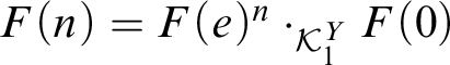 $F(n) = F(e)^n \cdot _{\mathcal {K}_1^Y} F(0)$
for every n. Write
$F(n) = F(e)^n \cdot _{\mathcal {K}_1^Y} F(0)$
for every n. Write
 $a = F(e)$
and
$a = F(e)$
and
 $b = F(0)$
. Notice then that
$b = F(0)$
. Notice then that
 $F \leqslant _{\mathrm {T}} Y$
via the computation
$F \leqslant _{\mathrm {T}} Y$
via the computation
 $n \mapsto a^n \cdot _{\mathcal {K}_1^Y} b$
.
$n \mapsto a^n \cdot _{\mathcal {K}_1^Y} b$
.
The characteristic function of X is X-computable, so there is an index
 $c \in \mathcal {K}_1^X$
such that for every n,
$c \in \mathcal {K}_1^X$
such that for every n,
 $$ \begin{align*} c \cdot_{\mathcal{K}_1^X} n = \begin{cases} 0 & \text{if }n \notin X, \\ 1 & \text{if }n \in X. \end{cases} \end{align*} $$
By applying F, we obtain an index
 $d = F(c)$
in
$d = F(c)$
in
 $\mathcal {K}_1^Y$
such that for every n,
$\mathcal {K}_1^Y$
such that for every n,
 $$ \begin{align*} d \cdot_{\mathcal{K}_1^Y} F(n) = \begin{cases} F(0) & \text{if }n \notin X, \\ F(1) & \text{if }n \in X. \end{cases} \end{align*} $$
It follows that
 $X \leqslant _{\mathrm {T}} Y$
because
$X \leqslant _{\mathrm {T}} Y$
because
 $F \leqslant _{\mathrm {T}} Y$
.⊣
$F \leqslant _{\mathrm {T}} Y$
.⊣
We now show that, for every
 $X \subseteq \omega $
,
$X \subseteq \omega $
,
 $\mathcal {K}_1^X$
embeds into
$\mathcal {K}_1^X$
embeds into
 $\mathcal {K}_2$
in a way that preserves
$\mathcal {K}_2$
in a way that preserves
 $\sim _\alpha $
for every ordinal
$\sim _\alpha $
for every ordinal
 $\alpha $
. An embedding
$\alpha $
. An embedding
 $F \colon \mathcal {A} \rightarrow \mathcal {B}$
of a pca
$F \colon \mathcal {A} \rightarrow \mathcal {B}$
of a pca
 $\mathcal {A}$
into a pca
$\mathcal {A}$
into a pca
 $\mathcal {B}$
extends to map from the closed terms over
$\mathcal {B}$
extends to map from the closed terms over
 $\mathcal {A}$
to the closed terms over
$\mathcal {A}$
to the closed terms over
 $\mathcal {B}$
by setting
$\mathcal {B}$
by setting
 $F(st) = F(s)F(t)$
for all closed terms s and t of
$F(st) = F(s)F(t)$
for all closed terms s and t of
 $\mathcal {A}$
. We define an embedding
$\mathcal {A}$
. We define an embedding
 $F \colon \mathcal {K}_1^X \rightarrow \mathcal {K}_2$
so that for every ordinal
$F \colon \mathcal {K}_1^X \rightarrow \mathcal {K}_2$
so that for every ordinal
 $\alpha $
and all closed terms s and t of
$\alpha $
and all closed terms s and t of
 $\mathcal {K}_1^X$
,
$\mathcal {K}_1^X$
,
 $s \sim _\alpha t$
in
$s \sim _\alpha t$
in
 $K_1^X$
if and only if
$K_1^X$
if and only if
 $F(s) \sim _\alpha F(t)$
in
$F(s) \sim _\alpha F(t)$
in
 $\mathcal {K}_2$
.
$\mathcal {K}_2$
.
Theorem 8.5. For every
 $X \subseteq \omega $
, there is an X-computable embedding
$X \subseteq \omega $
, there is an X-computable embedding
 $F \colon \mathcal {K}_1^X \rightarrow \mathcal {K}_2$
such that for all ordinals
$F \colon \mathcal {K}_1^X \rightarrow \mathcal {K}_2$
such that for all ordinals
 $\alpha $
and all closed terms s and t of
$\alpha $
and all closed terms s and t of
 $\mathcal {K}_1^X$
,
$\mathcal {K}_1^X$
,
 $s \sim _\alpha t$
in
$s \sim _\alpha t$
in
 $K_1^X$
if and only if
$K_1^X$
if and only if
 $F(s) \sim _\alpha F(t)$
in
$F(s) \sim _\alpha F(t)$
in
 $\mathcal {K}_2$
. The analogous statement with
$\mathcal {K}_2$
. The analogous statement with
 $\mathcal {K}_1$
in place of
$\mathcal {K}_1$
in place of
 $\mathcal {K}_1^X$
holds as well.
$\mathcal {K}_1^X$
holds as well.
Proof. We define an X-computable sequence
 $(f_n : n \in \omega )$
of elements of
$(f_n : n \in \omega )$
of elements of
 $\mathcal {K}_2$
with
$\mathcal {K}_2$
with
 $\langle n \rangle \sqsubseteq f_n$
for each n such that for all
$\langle n \rangle \sqsubseteq f_n$
for each n such that for all
 $a, b, c \in \mathcal {K}_1^X$
:
$a, b, c \in \mathcal {K}_1^X$
:
 $$ \begin{align*} a \cdot_{\mathcal{K}_1^X} b = c \quad&\Longrightarrow\quad \forall g \sqsupseteq \langle b \rangle \; (f_a \cdot_{\mathcal{K}_2} g = f_c), \\ (a \cdot_{\mathcal{K}_1^X} b){\uparrow} \quad&\Longrightarrow\quad \forall g \sqsupseteq \langle b \rangle \; (f_a \cdot_{\mathcal{K}_2} g){\uparrow}. \end{align*} $$
It follows that the map
 $F(a) = f_a$
embeds
$F(a) = f_a$
embeds
 $\mathcal {K}_1^X$
into
$\mathcal {K}_1^X$
into
 $\mathcal {K}_2$
because
$\mathcal {K}_2$
because
 $f_b \sqsupseteq \langle b \rangle $
for every b.
$f_b \sqsupseteq \langle b \rangle $
for every b.
It suffices to think of an element of
 $\mathcal {K}_2$
as a code for a total map
$\mathcal {K}_2$
as a code for a total map
 $\omega ^{<\omega } \rightarrow \omega ^{<\omega }$
, where if
$\omega ^{<\omega } \rightarrow \omega ^{<\omega }$
, where if
 $\sigma _0 \mapsto \tau _0$
,
$\sigma _0 \mapsto \tau _0$
,
 $\sigma _1 \mapsto \tau _1$
, and
$\sigma _1 \mapsto \tau _1$
, and
 $\sigma _0 \sqsubseteq \sigma _1$
, then also
$\sigma _0 \sqsubseteq \sigma _1$
, then also
 $\tau _0 \sqsubseteq \tau _1$
. If f codes such a map, then
$\tau _0 \sqsubseteq \tau _1$
. If f codes such a map, then
 $f \cdot _{\mathcal {K}_2} g = h$
if for every n there are a
$f \cdot _{\mathcal {K}_2} g = h$
if for every n there are a
 $\sigma \sqsubseteq g$
and a
$\sigma \sqsubseteq g$
and a
 $\tau \sqsubseteq h$
with
$\tau \sqsubseteq h$
with
 $|\tau | \geqslant n$
such that
$|\tau | \geqslant n$
such that
 $\sigma \mapsto \tau $
. If there is no such h for a given g, then
$\sigma \mapsto \tau $
. If there is no such h for a given g, then
 $(f \cdot _{\mathcal {K}_2} g) {\uparrow }$
. In the same way, finite strings are thought of as coding finite partial maps on strings. The only necessary detail from the encoding of
$(f \cdot _{\mathcal {K}_2} g) {\uparrow }$
. In the same way, finite strings are thought of as coding finite partial maps on strings. The only necessary detail from the encoding of
 $\mathcal {K}_2$
from [Reference Longley and Normann13, Section 3.2.1] we need is that if we assume
$\mathcal {K}_2$
from [Reference Longley and Normann13, Section 3.2.1] we need is that if we assume
 $0$
codes the empty string
$0$
codes the empty string
 $\epsilon $
, then the partial map coded by
$\epsilon $
, then the partial map coded by
 $\langle n \rangle $
is empty for every n.
$\langle n \rangle $
is empty for every n.
We define an X-computable sequence of finite strings
 $(f_{n,s} : n, s \in \omega )$
so that for each n,
$(f_{n,s} : n, s \in \omega )$
so that for each n,
 $\langle n \rangle = f_{n, 0} \sqsubseteq f_{n, 1} \sqsubseteq f_{n, 2} \sqsubseteq \cdots $
. In the end,
$\langle n \rangle = f_{n, 0} \sqsubseteq f_{n, 1} \sqsubseteq f_{n, 2} \sqsubseteq \cdots $
. In the end,
 $f_n = \bigcup _s f_{n, s}$
is the desired
$f_n = \bigcup _s f_{n, s}$
is the desired
 $f_n$
for each n. Start with
$f_n$
for each n. Start with
 $f_{n, 0} = \langle n \rangle $
for each n. At stage
$f_{n, 0} = \langle n \rangle $
for each n. At stage
 $s+1$
, consider each
$s+1$
, consider each
 $a \leqslant s$
and each string
$a \leqslant s$
and each string
 $\tau $
with code
$\tau $
with code
 $\leqslant s$
that is not yet in the domain of the partial map coded by
$\leqslant s$
that is not yet in the domain of the partial map coded by
 $f_{a, s}$
. If there are
$f_{a, s}$
. If there are
 $b, c \leqslant s$
with
$b, c \leqslant s$
with
 $\tau \sqsupseteq \langle b \rangle $
and
$\tau \sqsupseteq \langle b \rangle $
and
 $\Phi _{a,s}^X(b) {\downarrow } = c$
, then extend
$\Phi _{a,s}^X(b) {\downarrow } = c$
, then extend
 $f_{a, s}$
so as to map
$f_{a, s}$
so as to map
 $\tau $
to
$\tau $
to
 $f_{c,s}$
. Otherwise, extend
$f_{c,s}$
. Otherwise, extend
 $f_{a, s}$
so as to map
$f_{a, s}$
so as to map
 $\tau $
to
$\tau $
to
 $\epsilon $
. Let
$\epsilon $
. Let
 $f_{a, s+1}$
be the result of these extensions. Also, let
$f_{a, s+1}$
be the result of these extensions. Also, let
 $f_{n, s+1} = f_{n, s}$
for all
$f_{n, s+1} = f_{n, s}$
for all
 $n> s$
.
$n> s$
.
Suppose that
 $a \cdot _{\mathcal {K}_1^X} b = c$
, and let
$a \cdot _{\mathcal {K}_1^X} b = c$
, and let
 $s \geqslant a, b, c$
be large enough so that
$s \geqslant a, b, c$
be large enough so that
 $\Phi _{a, s}^X(b) = c$
. Then at every stage
$\Phi _{a, s}^X(b) = c$
. Then at every stage
 $t +1> s$
,
$t +1> s$
,
 $f_{a, t}$
is extended to map
$f_{a, t}$
is extended to map
 $\tau $
to
$\tau $
to
 $f_{c, t}$
whenever
$f_{c, t}$
whenever
 $\tau \sqsupseteq \langle b \rangle $
,
$\tau \sqsupseteq \langle b \rangle $
,
 $\tau \leqslant t$
, and
$\tau \leqslant t$
, and
 $\tau $
is not already in the domain of the partial map coded by
$\tau $
is not already in the domain of the partial map coded by
 $f_{a,t}$
. Therefore
$f_{a,t}$
. Therefore
 $f_a \cdot _{\mathcal {K}_2} g = f_c$
for all
$f_a \cdot _{\mathcal {K}_2} g = f_c$
for all
 $g \sqsupseteq \langle b \rangle $
.
$g \sqsupseteq \langle b \rangle $
.
Conversely, suppose that
 $(a \cdot _{\mathcal {K}_1^X} b){\uparrow }$
. Then for every s,
$(a \cdot _{\mathcal {K}_1^X} b){\uparrow }$
. Then for every s,
 $f_{a,s}$
maps
$f_{a,s}$
maps
 $\tau $
to
$\tau $
to
 $\epsilon $
whenever
$\epsilon $
whenever
 $\tau \sqsupseteq \langle b \rangle $
is in the domain of the partial function coded by
$\tau \sqsupseteq \langle b \rangle $
is in the domain of the partial function coded by
 $f_{a,s}$
. Thus
$f_{a,s}$
. Thus
 $(f_a \cdot _{\mathcal {K}_2} g){\uparrow }$
for all
$(f_a \cdot _{\mathcal {K}_2} g){\uparrow }$
for all
 $g \sqsupseteq \langle b \rangle $
.
$g \sqsupseteq \langle b \rangle $
.
We now show that the embedding F preserves
 $\sim _\alpha $
. First, we have that for every closed term t over
$\sim _\alpha $
. First, we have that for every closed term t over
 $\mathcal {K}_1$
and every
$\mathcal {K}_1$
and every
 $b, c \in \mathcal {K}_1^X$
:
$b, c \in \mathcal {K}_1^X$
:
 $$ \begin{align*} t \cdot_{\mathcal{K}_1^X} b = c \quad&\Longrightarrow\quad \forall g \sqsupseteq \langle b \rangle \; (F(t) \cdot_{\mathcal{K}_2} g = F(c)), \\ (t \cdot_{\mathcal{K}_1^X} b){\uparrow} \quad&\Longrightarrow\quad \forall g \sqsupseteq \langle b \rangle \; (F(t) \cdot_{\mathcal{K}_2} g){\uparrow}. \end{align*} $$
This is because if
 $t{\downarrow } = a$
then
$t{\downarrow } = a$
then
 $F(t){\downarrow } = F(a)$
, so the implications for t follow from the corresponding implications for a. On the other hand, if
$F(t){\downarrow } = F(a)$
, so the implications for t follow from the corresponding implications for a. On the other hand, if
 $t {\uparrow }$
, then
$t {\uparrow }$
, then
 $F(t) {\uparrow }$
as well, from which the implications follow. Therefore, if t is a closed term over
$F(t) {\uparrow }$
as well, from which the implications follow. Therefore, if t is a closed term over
 $\mathcal {K}_1^X$
and
$\mathcal {K}_1^X$
and
 $g \in \mathcal {K}_2$
, then
$g \in \mathcal {K}_2$
, then
 $F(t) \cdot _{\mathcal {K}_2} g \sim _0 F(t) \cdot _{\mathcal {K}_2} F(b)$
, where
$F(t) \cdot _{\mathcal {K}_2} g \sim _0 F(t) \cdot _{\mathcal {K}_2} F(b)$
, where
 $b = g(0)$
.
$b = g(0)$
.
Now proceed by transfinite induction on
 $\alpha $
. For the base case, we have that
$\alpha $
. For the base case, we have that
 $s \sim _0 t$
in
$s \sim _0 t$
in
 $\mathcal {K}_1^X$
if and only if
$\mathcal {K}_1^X$
if and only if
 $F(s) \sim _0 F(t)$
in
$F(s) \sim _0 F(t)$
in
 $\mathcal {K}_2$
for all closed terms s and t of
$\mathcal {K}_2$
for all closed terms s and t of
 $\mathcal {K}_1^X$
because F is an embedding.
$\mathcal {K}_1^X$
because F is an embedding.
For the successor case, assume that
 $s \sim _\alpha t$
in
$s \sim _\alpha t$
in
 $\mathcal {K}_1^X$
if and only if
$\mathcal {K}_1^X$
if and only if
 $F(s) \sim _\alpha F(t)$
in
$F(s) \sim _\alpha F(t)$
in
 $\mathcal {K}_2$
for all closed terms s and t of
$\mathcal {K}_2$
for all closed terms s and t of
 $\mathcal {K}_1^X$
. Now consider two closed terms s and t of
$\mathcal {K}_1^X$
. Now consider two closed terms s and t of
 $\mathcal {K}_1^X$
. Suppose that
$\mathcal {K}_1^X$
. Suppose that
 $s \sim _{\alpha + 1} t$
in
$s \sim _{\alpha + 1} t$
in
 $\mathcal {K}_1^X$
. We want to show that
$\mathcal {K}_1^X$
. We want to show that
 $F(s) \sim _{\alpha + 1} F(t)$
in
$F(s) \sim _{\alpha + 1} F(t)$
in
 $\mathcal {K}_2$
. Let
$\mathcal {K}_2$
. Let
 $g \in \mathcal {K}_2$
, and let
$g \in \mathcal {K}_2$
, and let
 $b = g(0)$
. Then
$b = g(0)$
. Then
 $s b \sim _\alpha t b$
because
$s b \sim _\alpha t b$
because
 $s \sim _{\alpha + 1} t$
, so therefore
$s \sim _{\alpha + 1} t$
, so therefore
 $F(s b) \sim _\alpha F(t b)$
. Thus,
$F(s b) \sim _\alpha F(t b)$
. Thus,
 $$ \begin{align*} F(s) \cdot_{\mathcal{K}_2} g \sim_0 F(s) \cdot_{\mathcal{K}_2} F(b) \sim_0 F(s b) \sim_\alpha F(t b) \sim_0 F(t) \cdot_{\mathcal{K}_2} F(b) \sim_0 F(t) \cdot_{\mathcal{K}_2} g. \end{align*} $$
Thus
 $F(s) \cdot _{\mathcal {K}_2} g \sim _\alpha F(t) \cdot _{\mathcal {K}_2} g$
for every
$F(s) \cdot _{\mathcal {K}_2} g \sim _\alpha F(t) \cdot _{\mathcal {K}_2} g$
for every
 $g \in \mathcal {K}_2$
, so
$g \in \mathcal {K}_2$
, so
 $F(s) \sim _{\alpha + 1} F(t)$
. Conversely, suppose that
$F(s) \sim _{\alpha + 1} F(t)$
. Conversely, suppose that
 $s \not \sim _{\alpha + 1} t$
in
$s \not \sim _{\alpha + 1} t$
in
 $\mathcal {K}_1^X$
. Then there is a
$\mathcal {K}_1^X$
. Then there is a
 $b \in \mathcal {K}_1^X$
such that
$b \in \mathcal {K}_1^X$
such that
 $s b \not \sim _\alpha t b$
. Then
$s b \not \sim _\alpha t b$
. Then
 $F(s b) \not \sim _\alpha F(t b)$
by the induction hypothesis, so
$F(s b) \not \sim _\alpha F(t b)$
by the induction hypothesis, so
 $$ \begin{align*} F(s) \cdot_{\mathcal{K}_2} F(b) \sim_0 F(s b) \not\sim_\alpha F(t b) \sim_0 F(t) \cdot_{\mathcal{K}_2} F(b). \end{align*} $$
Thus
 $F(s) \not \sim _{\alpha + 1} F(t)$
.
$F(s) \not \sim _{\alpha + 1} F(t)$
.
The limit case follows easily from the inductive hypothesis, which completes the proof.
The proof for
 $\mathcal {K}_1$
in place of
$\mathcal {K}_1$
in place of
 $\mathcal {K}_1^X$
is the same, with plain Turing machines in place of oracle Turing machines.⊣
$\mathcal {K}_1^X$
is the same, with plain Turing machines in place of oracle Turing machines.⊣
Definition 8.6. For a pca
 $\mathcal {A}$
and closed terms s and t over
$\mathcal {A}$
and closed terms s and t over
 $\mathcal {A}$
, let
$\mathcal {A}$
, let
 $$ \begin{align*} \mathrm{ord}_{\mathcal{A}}(s, t) = \begin{cases} \text{the least ordinal }\alpha\text{ such that }s \sim_\alpha t & \text{if }s \approx t, \\ \infty & \text{if }s \not\approx t. \end{cases} \end{align*} $$
Here
 $\infty $
is a new symbol, and we define
$\infty $
is a new symbol, and we define
 $\alpha < \infty $
for every ordinal
$\alpha < \infty $
for every ordinal
 $\alpha $
. Notice that
$\alpha $
. Notice that
 $$ \begin{align*} \mathrm{ord}(\mathcal{A}) = \sup\{\mathrm{ord}_{\mathcal{A}}(s, t) : s \text{ and } t \text{ are closed terms over }\mathcal{A} \text{ with } \mathrm{ord}_{\mathcal{A}}(s, t) < \infty\}, \end{align*} $$
by the discussion following Definition 3.6. Furthermore, if
 $\mathcal {A}$
is not extensional, then
$\mathcal {A}$
is not extensional, then
 $$ \begin{align*} \mathrm{ord}(\mathcal{A}) = \sup\{\mathrm{ord}_{\mathcal{A}}(a, b) : a, b \in \mathcal{A} \wedge \mathrm{ord}_{\mathcal{A}}(a, b) < \infty\}. \end{align*} $$
If
 $\mathcal {A}$
is a sub-pca of
$\mathcal {A}$
is a sub-pca of
 $\mathcal {B}$
, then
$\mathcal {B}$
, then
 $\mathrm {ord}(\mathcal {A}) \leqslant \mathrm {ord}(\mathcal {B})$
, provided that
$\mathrm {ord}(\mathcal {A}) \leqslant \mathrm {ord}(\mathcal {B})$
, provided that
 $\mathrm {ord}_{\mathcal {B}}(s, t) < \infty $
whenever s and t are closed terms over
$\mathrm {ord}_{\mathcal {B}}(s, t) < \infty $
whenever s and t are closed terms over
 $\mathcal {A}$
with
$\mathcal {A}$
with
 $\mathrm {ord}_{\mathcal {A}}(s, t) < \infty $
.
$\mathrm {ord}_{\mathcal {A}}(s, t) < \infty $
.
Proposition 8.7. Let
 $\mathcal {A}$
and
$\mathcal {A}$
and
 $\mathcal {B}$
be pca’s with
$\mathcal {B}$
be pca’s with
 $\mathcal {A}$
a sub-pca of
$\mathcal {A}$
a sub-pca of
 $\mathcal {B}$
.
$\mathcal {B}$
.
-
(i) For all closed terms s and t over
$\mathcal {A}$
,
$\mathrm {ord}_{\mathcal {A}}(s,t) \leqslant \mathrm {ord}_{\mathcal {B}}(s,t)$
. -
(ii) If
$\mathrm {ord}_{\mathcal {A}}(s,t) < \infty \Longrightarrow \mathrm {ord}_{\mathcal {B}}(s,t) < \infty $
for all closed terms s and t over
$\mathcal {A}$
, then
$\mathrm {ord}(\mathcal {A}) \leqslant \mathrm {ord}(\mathcal {B})$
. -
(iii) If
$\mathcal {A}$
and
$\mathcal {B}$
are non-extensional and
$\mathrm {ord}_{\mathcal {A}}(a,b) < \infty \Longrightarrow \mathrm {ord}_{\mathcal {B}}(a,b) < \infty $
for all
$a, b \in \mathcal {A}$
, then
$\mathrm {ord}(\mathcal {A}) \leqslant \mathrm {ord}(\mathcal {B})$
.


Proof. For i, a straightforward transfinite induction on
 $\alpha $
shows that for all ordinals
$\alpha $
shows that for all ordinals
 $\alpha $
and all closed terms s and t over
$\alpha $
and all closed terms s and t over
 $\mathcal {A}$
, if
$\mathcal {A}$
, if
 $s \sim _\alpha t$
in
$s \sim _\alpha t$
in
 $\mathcal {B}$
, then
$\mathcal {B}$
, then
 $s \sim _\alpha t$
in
$s \sim _\alpha t$
in
 $\mathcal {A}$
. Thus for any fixed closed terms s and t over
$\mathcal {A}$
. Thus for any fixed closed terms s and t over
 $\mathcal {A}$
, either
$\mathcal {A}$
, either
 $\mathrm {ord}_{\mathcal {B}}(s,t) = \infty $
, in which case i trivially holds; or
$\mathrm {ord}_{\mathcal {B}}(s,t) = \infty $
, in which case i trivially holds; or
 $\mathrm {ord}_{\mathcal {B}}(s,t) < \infty $
, in which case
$\mathrm {ord}_{\mathcal {B}}(s,t) < \infty $
, in which case
 $s \sim _{\mathrm {ord}_{\mathcal {B}}(s,t)} t$
in both
$s \sim _{\mathrm {ord}_{\mathcal {B}}(s,t)} t$
in both
 $\mathcal {A}$
and
$\mathcal {A}$
and
 $\mathcal {B}$
, so
$\mathcal {B}$
, so
 $\mathrm {ord}_{\mathcal {A}}(s,t) \leqslant \mathrm {ord}_{\mathcal {B}}(s, t)$
.
$\mathrm {ord}_{\mathcal {A}}(s,t) \leqslant \mathrm {ord}_{\mathcal {B}}(s, t)$
.
For ii, assume that
 $\mathrm {ord}_{\mathcal {A}}(s,t) < \infty \Longrightarrow \mathrm {ord}_{\mathcal {B}}(s,t) < \infty $
for all closed terms s and t over
$\mathrm {ord}_{\mathcal {A}}(s,t) < \infty \Longrightarrow \mathrm {ord}_{\mathcal {B}}(s,t) < \infty $
for all closed terms s and t over
 $\mathcal {A}$
. Then by i:
$\mathcal {A}$
. Then by i:
 $$ \begin{align*} \mathrm{ord}(\mathcal{A}) &= \sup\{\mathrm{ord}_{\mathcal{A}}(s, t) : s \text{ and }t \text{ are closed terms over } \mathcal{A} \text{ with }\mathrm{ord}_{\mathcal{A}}(s, t) < \infty\} \\ &\leqslant \sup\{\mathrm{ord}_{\mathcal{B}}(s, t) : s \text{ and }t \text{ are closed terms over } \mathcal{A} \text{ with } \mathrm{ord}_{\mathcal{B}}(s, t) < \infty\} \\ &\leqslant \sup\{\mathrm{ord}_{\mathcal{B}}(s, t) : s \text{ and }t \text{ are closed terms over }\mathcal{B} \text{ with } \mathrm{ord}_{\mathcal{B}}(s, t) < \infty\} \\ &=\mathrm{ord}(\mathcal{B}). \end{align*} $$
For iii, if
 $\mathcal {A}$
and
$\mathcal {A}$
and
 $\mathcal {B}$
are non-extensional, then we can give the same argument as in ii but with elements of the algebras in place of more general closed terms.⊣
$\mathcal {B}$
are non-extensional, then we can give the same argument as in ii but with elements of the algebras in place of more general closed terms.⊣
9 Ordinal analysis of
$\mathcal {K}_2$

In this section we use the results of Section 8 to prove that the closure ordinal of Kleene’s second model
 $\mathcal {K}_2$
is equal to
$\mathcal {K}_2$
is equal to
 $\omega _1$
.
$\omega _1$
.
Theorem 9.1.
 $\mathrm {ord}(\mathcal {K}_2) = \omega _1$
.
$\mathrm {ord}(\mathcal {K}_2) = \omega _1$
.
Proof. The proof that
 $\mathrm {ord}(\mathcal {K}_2) \leqslant \omega _1$
follows the proof of Theorem 5.4. Let
$\mathrm {ord}(\mathcal {K}_2) \leqslant \omega _1$
follows the proof of Theorem 5.4. Let
 $\Omega $
denote the set of closed terms over
$\Omega $
denote the set of closed terms over
 $\mathcal {K}_2$
, coded as elements of
$\mathcal {K}_2$
, coded as elements of
 $\omega ^\omega $
in some effective way. Notice that
$\omega ^\omega $
in some effective way. Notice that
 $s \simeq t$
is an arithmetical property of (the codes for) s and t.
$s \simeq t$
is an arithmetical property of (the codes for) s and t.
Consider the operator
 $\Gamma \colon {\mathcal P}(\Omega \times \Omega ) \rightarrow {\mathcal P}(\Omega \times \Omega )$
defined by
$\Gamma \colon {\mathcal P}(\Omega \times \Omega ) \rightarrow {\mathcal P}(\Omega \times \Omega )$
defined by
 $$ \begin{align*} \Gamma(X) = \big\{ (s, t) \in \Omega\times\Omega : \forall x \in \mathcal{K}_2 \; (s x, t x) \in X \big\}. \end{align*} $$
Define
 $\Gamma _\alpha $
for every ordinal
$\Gamma _\alpha $
for every ordinal
 $\alpha $
by
$\alpha $
by
 $$ \begin{align*} \Gamma_0 &= \big\{ (s,t) : s \simeq t \big\}, \\ \Gamma_{\alpha+1} &= \Gamma(\Gamma_\alpha), \\ \Gamma_\gamma &= \bigcup_{\alpha < \gamma} \Gamma_\alpha, \hspace{1cm} \text{for }\gamma\text{ a limit ordinal.} \end{align*} $$
Then for closed terms s and t,
 $s \sim _\alpha t$
if and only if
$s \sim _\alpha t$
if and only if
 $(s, t) \in \Gamma _\alpha $
.
$(s, t) \in \Gamma _\alpha $
.
We observe that the operator
 $\Gamma $
is
$\Gamma $
is
 $\Pi ^1_1$
and monotone. Since X is now a subset of
$\Pi ^1_1$
and monotone. Since X is now a subset of
 $\omega ^\omega $
, this has to be understood in terms of Kleene’s recursion in higher types. The predicate
$\omega ^\omega $
, this has to be understood in terms of Kleene’s recursion in higher types. The predicate
 $(s x, t x) \in X$
is indeed recursive in X, as it requires only one oracle query to X. The closure ordinal for
$(s x, t x) \in X$
is indeed recursive in X, as it requires only one oracle query to X. The closure ordinal for
 $\Pi ^1_1$
monotone operators such as
$\Pi ^1_1$
monotone operators such as
 $\Gamma $
is at most
$\Gamma $
is at most
 $\omega _1$
by Cenzer [Reference Cenzer7, Theorem 4.1] (see also [Reference Sacks21, Corollary III.8.10]), so
$\omega _1$
by Cenzer [Reference Cenzer7, Theorem 4.1] (see also [Reference Sacks21, Corollary III.8.10]), so
 $\mathrm {ord}(\mathcal {K}_2) \leqslant \omega _1$
.
$\mathrm {ord}(\mathcal {K}_2) \leqslant \omega _1$
.
One may show that
 $\omega _1 \leqslant \mathrm {ord}(\mathcal {K}_2)$
by constructing for each
$\omega _1 \leqslant \mathrm {ord}(\mathcal {K}_2)$
by constructing for each
 $\alpha < \omega _1$
elements
$\alpha < \omega _1$
elements
 $f_\alpha $
and
$f_\alpha $
and
 $g_\alpha $
of
$g_\alpha $
of
 $\mathcal {K}_2$
such that
$\mathcal {K}_2$
such that
 $f_\alpha \not \sim _\alpha g_\alpha $
and
$f_\alpha \not \sim _\alpha g_\alpha $
and
 $f_\alpha \sim _{\alpha +1} g_\alpha $
in a similar spirit to the proof of Theorem 5.1. At successor stages, take
$f_\alpha \sim _{\alpha +1} g_\alpha $
in a similar spirit to the proof of Theorem 5.1. At successor stages, take
 $f_{\alpha + 1} = K f_\alpha $
and
$f_{\alpha + 1} = K f_\alpha $
and
 $g_{\alpha + 1} = K g_\alpha $
as before. At limit stages, choose a sequence of ordinals
$g_{\alpha + 1} = K g_\alpha $
as before. At limit stages, choose a sequence of ordinals
 $\beta _0 < \beta _1 < \beta _2 < \cdots $
with
$\beta _0 < \beta _1 < \beta _2 < \cdots $
with
 $\alpha = \lim _n \beta _n$
, and directly define
$\alpha = \lim _n \beta _n$
, and directly define
 $f_\alpha $
and
$f_\alpha $
and
 $g_\alpha $
so that
$g_\alpha $
so that
 $f_\alpha \cdot h = f_{\beta _{h(0)}}$
and
$f_\alpha \cdot h = f_{\beta _{h(0)}}$
and
 $g_\alpha \cdot h = g_{\beta _{h(0)}}$
for all
$g_\alpha \cdot h = g_{\beta _{h(0)}}$
for all
 $h \in \mathcal {K}_2$
. Instead, we use the embeddings of
$h \in \mathcal {K}_2$
. Instead, we use the embeddings of
 $\mathcal {K}_1^X$
into
$\mathcal {K}_1^X$
into
 $\mathcal {K}_2$
for
$\mathcal {K}_2$
for
 $X \subseteq \omega $
to show that
$X \subseteq \omega $
to show that
 $\omega _1 \leqslant \mathrm {ord}(\mathcal {K}_2)$
. Thus consider any
$\omega _1 \leqslant \mathrm {ord}(\mathcal {K}_2)$
. Thus consider any
 $X \subseteq \omega $
and the embedding
$X \subseteq \omega $
and the embedding
 $F \colon \mathcal {K}_1^X \rightarrow \mathcal {K}_2$
of Theorem 8.5. Identify
$F \colon \mathcal {K}_1^X \rightarrow \mathcal {K}_2$
of Theorem 8.5. Identify
 $\mathcal {K}_1^X$
with its image under F in order to view
$\mathcal {K}_1^X$
with its image under F in order to view
 $\mathcal {K}_1^X$
as a sub-pca of
$\mathcal {K}_1^X$
as a sub-pca of
 $\mathcal {K}_2$
. Then Theorem 8.5 tells us that for all ordinals
$\mathcal {K}_2$
. Then Theorem 8.5 tells us that for all ordinals
 $\alpha $
and all closed terms s and t over
$\alpha $
and all closed terms s and t over
 $\mathcal {K}_1^X$
,
$\mathcal {K}_1^X$
,
 $s \sim _\alpha t$
in
$s \sim _\alpha t$
in
 $\mathcal {K}_1^X$
if and only if
$\mathcal {K}_1^X$
if and only if
 $s \sim _\alpha t$
in
$s \sim _\alpha t$
in
 $\mathcal {K}_2$
. In particular,
$\mathcal {K}_2$
. In particular,
 $\mathrm {ord}_{\mathcal {K}_1^X}(s,t) < \infty \Longrightarrow \mathrm {ord}_{\mathcal {K}_2}(s,t) < \infty $
for all closed terms s and t over
$\mathrm {ord}_{\mathcal {K}_1^X}(s,t) < \infty \Longrightarrow \mathrm {ord}_{\mathcal {K}_2}(s,t) < \infty $
for all closed terms s and t over
 $\mathcal {K}_1^X$
. Therefore
$\mathcal {K}_1^X$
. Therefore
 $\mathrm {ord}(\mathcal {K}_1^X) \leqslant \mathrm {ord}(\mathcal {K}_2)$
by Proposition 8.7. Furthermore,
$\mathrm {ord}(\mathcal {K}_1^X) \leqslant \mathrm {ord}(\mathcal {K}_2)$
by Proposition 8.7. Furthermore,
 $\mathrm {ord}(\mathcal {K}_1^X) = \omega _1^X$
by Theorem 5.5 relativized to X. Thus
$\mathrm {ord}(\mathcal {K}_1^X) = \omega _1^X$
by Theorem 5.5 relativized to X. Thus
 $\omega _1^X \leqslant \mathrm {ord}(\mathcal {K}_2)$
for every X. Now the supremum of the
$\omega _1^X \leqslant \mathrm {ord}(\mathcal {K}_2)$
for every X. Now the supremum of the
 $\omega _1^X$
is
$\omega _1^X$
is
 $\omega _1$
, because every
$\omega _1$
, because every
 $\alpha <\omega _1$
is X-computable for some X, hence
$\alpha <\omega _1$
is X-computable for some X, hence
 $\omega _1 \leqslant \mathrm {ord}(\mathcal {K}_2)$
.⊣
$\omega _1 \leqslant \mathrm {ord}(\mathcal {K}_2)$
.⊣
Consider any f and g in
 $\mathcal {K}_2$
, and let
$\mathcal {K}_2$
, and let
 $\Gamma $
be as in the proof of Theorem 9.1. By Cenzer [Reference Cenzer7, Proposition 4.9] (see also [Reference Sacks21, Theorem III.8.9]), if
$\Gamma $
be as in the proof of Theorem 9.1. By Cenzer [Reference Cenzer7, Proposition 4.9] (see also [Reference Sacks21, Theorem III.8.9]), if
 $(f, g) \in \Gamma _\alpha $
for some
$(f, g) \in \Gamma _\alpha $
for some
 $\alpha $
, then
$\alpha $
, then
 $(f, g) \in \Gamma _\alpha $
for an
$(f, g) \in \Gamma _\alpha $
for an
 $\alpha < \omega _1^{f \oplus g}$
. That is, if
$\alpha < \omega _1^{f \oplus g}$
. That is, if
 $f \approx g$
in
$f \approx g$
in
 $\mathcal {K}_2$
, then
$\mathcal {K}_2$
, then
 $f \sim _{\omega _1^{f \oplus g}} g$
. It would be interesting to give a fine analysis of the
$f \sim _{\omega _1^{f \oplus g}} g$
. It would be interesting to give a fine analysis of the
 $\sim _\alpha $
relations for
$\sim _\alpha $
relations for
 $\alpha < \omega _1$
on
$\alpha < \omega _1$
on
 $\mathcal {K}_2$
, but we do not pursue this direction here.
$\mathcal {K}_2$
, but we do not pursue this direction here.
We conclude this section with a remark about the effective version of
 $\mathcal {K}_2$
. This version is called
$\mathcal {K}_2$
. This version is called
 $\mathcal {K}_2^{\mathrm {eff}}$
in Longley and Norman [Reference Longley and Normann13], and it is obtained by restricting
$\mathcal {K}_2^{\mathrm {eff}}$
in Longley and Norman [Reference Longley and Normann13], and it is obtained by restricting
 $\mathcal {K}_2$
to total computable elements
$\mathcal {K}_2$
to total computable elements
 $f\in \omega ^\omega $
. This is again a pca because the combinators K and S in
$f\in \omega ^\omega $
. This is again a pca because the combinators K and S in
 $\mathcal {K}_2$
are computable.
$\mathcal {K}_2$
are computable.
Theorem 9.2.
 $\mathrm {ord}(\mathcal {K}_2^{\mathrm {eff}}) = {\omega _1^{\textit {CK}}}$
.
$\mathrm {ord}(\mathcal {K}_2^{\mathrm {eff}}) = {\omega _1^{\textit {CK}}}$
.
Proof. Using
 $\emptyset ^{\prime \prime }$
, we can index the total computable functions and partially compute the partial application operation of
$\emptyset ^{\prime \prime }$
, we can index the total computable functions and partially compute the partial application operation of
 $\mathcal {K}_2^{\mathrm {eff}}$
. Therefore
$\mathcal {K}_2^{\mathrm {eff}}$
. Therefore
 $\mathrm {ord}(\mathcal {K}_2^{\mathrm {eff}}) \leqslant \omega _1^{\emptyset ^{\prime \prime }} = {\omega _1^{\textit {CK}}}$
, where the inequality is by Theorem 5.8 and the equality is by [Reference Sacks21, Corollary II.7.4]. The reverse inequality
$\mathrm {ord}(\mathcal {K}_2^{\mathrm {eff}}) \leqslant \omega _1^{\emptyset ^{\prime \prime }} = {\omega _1^{\textit {CK}}}$
, where the inequality is by Theorem 5.8 and the equality is by [Reference Sacks21, Corollary II.7.4]. The reverse inequality
 ${\omega _1^{\textit {CK}}} \leqslant \mathrm {ord}(\mathcal {K}_2^{\mathrm {eff}})$
can be proved in the same way as Theorem 9.1. The embedding
${\omega _1^{\textit {CK}}} \leqslant \mathrm {ord}(\mathcal {K}_2^{\mathrm {eff}})$
can be proved in the same way as Theorem 9.1. The embedding
 $F \colon \mathcal {K}_1 \rightarrow \mathcal {K}_2$
of Theorem 8.5 produces computable elements of
$F \colon \mathcal {K}_1 \rightarrow \mathcal {K}_2$
of Theorem 8.5 produces computable elements of
 $\mathcal {K}_2$
. Thus F embeds
$\mathcal {K}_2$
. Thus F embeds
 $\mathcal {K}_1$
into
$\mathcal {K}_1$
into
 $\mathcal {K}_2^{\mathrm {eff}}$
. By inspecting the proof of Theorem 8.5, we see that again for all ordinals
$\mathcal {K}_2^{\mathrm {eff}}$
. By inspecting the proof of Theorem 8.5, we see that again for all ordinals
 $\alpha $
and all closed terms s and t of
$\alpha $
and all closed terms s and t of
 $\mathcal {K}_1$
,
$\mathcal {K}_1$
,
 $s \sim _\alpha t$
in
$s \sim _\alpha t$
in
 $\mathcal {K}_1$
if and only if
$\mathcal {K}_1$
if and only if
 $F(s) \sim _\alpha F(t)$
in
$F(s) \sim _\alpha F(t)$
in
 $\mathcal {K}_2^{\mathrm {eff}}$
. The proof now proceeds as in that of Theorem 9.1, and we conclude that
$\mathcal {K}_2^{\mathrm {eff}}$
. The proof now proceeds as in that of Theorem 9.1, and we conclude that
 ${\omega _1^{\textit {CK}}} = \mathrm {ord}(\mathcal {K}_1) \leqslant \mathrm {ord}(\mathcal {K}_2^{\mathrm {eff}})$
.⊣
${\omega _1^{\textit {CK}}} = \mathrm {ord}(\mathcal {K}_1) \leqslant \mathrm {ord}(\mathcal {K}_2^{\mathrm {eff}})$
.⊣
Acknowledgments
The authors thank Emanuele Frittaion, Russell Miller, and Michael Rathjen for helpful discussions. This project was partially supported by a grant from the John Templeton Foundation (A new dawn of intuitionism: mathematical and philosophical advances ID 60842). The opinions expressed in this work are those of the authors and do not necessarily reflect the views of the John Templeton Foundation.


 Open access