


1. Introduction
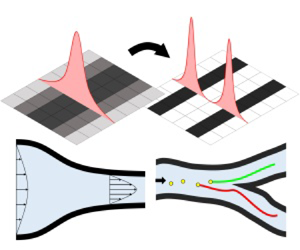
This study develops a new density filter for designing pipe-shaped structures for fluid topology optimization. The pipe-shaped structure consisted of a pipe wall, an outer pipe region and an inner pipe region where fluid flows (figure 1). In traditional fluid topology optimization, the resulting structure consists of pseudo-solid and fluid domains. A postprocessing step is usually required to transform this design into a manufacturable structure. However, with the scheme presented in this paper, a manufacturable design is directly obtained without additional postprocessing. Moreover, unlike the approach of simply optimizing and then postprocessing, this scheme allows the optimization of parameters such as pipe thickness and cross-sectional area. An inherent feature of this approach makes it possible to impose constraints pertaining to the thickness and cross-sectional area. This paper presents a topology optimization method that can be used to directly design optimal pipe-shaped structures.

Figure 1. Concept of the pipe density filter and its application to fluid problems. (a) Conventional fluid topology optimization, (b) pipe structure, (c) two topology optimizations with the pipe density filter and (d) pipe wall thickness and pipe cross-sectional thickness.
Topology optimization is a versatile scheme extensively used in various fields. Several topology optimization schemes have been developed for structural optimization, such as the solid isotropic material with penalization (SIMP), the level-set and the moving morphable component methods (Bendsøe & Kikuchi Reference Bendsøe and Kikuchi1988; Wang, Wang & Guo Reference Wang, Wang and Guo2003; Zhang et al. Reference Zhang, Yuan, Zhang and Guo2016). Additionally, topology optimization has been extensively studied in multiphysics systems, including fluid systems, fluid–particle interaction and fluid–structure interaction (Borrvall & Petersson Reference Borrvall and Petersson2003; Gersborg-Hansen, Sigmund & Haber Reference Gersborg-Hansen, Sigmund and Haber2005; Aage et al. Reference Aage, Poulsen, Gersborg-Hansen and Sigmund2008; Yoon Reference Yoon2010, Reference Yoon2022; Deng et al. Reference Deng, Liu, Zhang, Liu and Wu2011; Andreasen & Sigmund Reference Andreasen and Sigmund2013; Jenkins & Maute Reference Jenkins and Maute2015, Reference Jenkins and Maute2016; Chen Reference Chen2016; Picelli, Vicente & Pavanello Reference Picelli, Vicente and Pavanello2017; Lundgaard et al. Reference Lundgaard, Alexandersen, Zhou, Andreasen and Sigmund2018; Andreasen Reference Andreasen2020; Picelli et al. Reference Picelli, Ranjbarzadeh, Sivapuram, Gioria and Silva2020; Yoon Reference Yoon2020; Yoon & So Reference Yoon and So2021). In Borrvall & Petersson (Reference Borrvall and Petersson2003), topology optimization was proposed to minimize the fluid energy dissipation in Stokes flow. In Gersborg-Hansen et al. (Reference Gersborg-Hansen, Sigmund and Haber2005), fluid topology optimization was considered in steady-state incompressible viscous flow. In Aage et al. (Reference Aage, Poulsen, Gersborg-Hansen and Sigmund2008), it was applied to the large-scale fluid problem. In Deng et al. (Reference Deng, Liu, Zhang, Liu and Wu2011), topology optimization for unsteady flow was proposed. A variety of other fluid topology optimization schemes were reviewed in Chen (Reference Chen2016). Recently, topology optimization has been used to control particles suspended in fluid (Andreasen Reference Andreasen2020; Yoon Reference Yoon2020; Yoon & So Reference Yoon and So2021; Yoon Reference Yoon2022; Choi & Yoon Reference Choi and Yoon2023). In Yoon (Reference Yoon2020) and Andreasen (Reference Andreasen2020), a topology optimization was conducted to control particles in steady-state fluid, and the sensitivity was derived. Multiple particles in fluid were controlled through topology optimization using the SHAKE algorithm (Yoon & So Reference Yoon and So2021). The topology optimization of particles in unsteady fluid flow was presented in Yoon (Reference Yoon2022). As stated above, fluid topology optimization is an actively studied field. Among these investigations, the new density filter can be applied to both traditional fluid topology optimization and fluid–particle topology optimization, which is also actively being researched (Andreasen Reference Andreasen2020; Yoon Reference Yoon2020; Yoon & So Reference Yoon and So2021; Yoon Reference Yoon2022; Choi & Yoon Reference Choi and Yoon2023). Recent studies in the field of topology optimization have explored a wide range of areas, including the optimization of fluid systems and the control of particles within a fluid.
As previously mentioned, there has been much progress in topology optimization, and more recently, studies have focused on manufacturability. The focus on manufacturability has already been actively investigated in the field of structural topology optimization, such as coating structures and a thin-wall-shaped structure (Clausen, Aage & Sigmund Reference Clausen, Aage and Sigmund2015; Wang & Kang Reference Wang and Kang2018; Fu et al. Reference Fu, Li, Gao and Xiao2019a,Reference Fu, Li, Xiao, Gao and Chub; Yoon & Yi Reference Yoon and Yi2019; Zhou et al. Reference Zhou, Nomura, Dede and Saitou2022). In Clausen et al. (Reference Clausen, Aage and Sigmund2015), the topology optimization of coating structures was presented. Level-set methods for coating structures were proposed (Wang & Kang Reference Wang and Kang2018; Fu et al. Reference Fu, Li, Gao and Xiao2019a,Reference Fu, Li, Xiao, Gao and Chub). Coating structures were designed using density-based topology optimization with a coating filter (Yoon & Yi Reference Yoon and Yi2019). Moreover, topology optimization for a thin-wall-shaped foldable structure was studied (Zhou et al. Reference Zhou, Nomura, Dede and Saitou2022). Furthermore, to prevent the structure from becoming too thin, the use of a geometric constraint to control the minimum length scale was investigated (Zhou et al. Reference Zhou, Lazarov, Wang and Sigmund2015; Zhao et al. Reference Zhao, Zhou, Sigmund and Andreasen2018). Controlling the maximum length scale was also researched (Zhang, Zhong & Guo Reference Zhang, Zhong and Guo2014; Lazarov & Wang Reference Lazarov and Wang2017). In Kim & Yoon (Reference Kim and Yoon2000), the wavelet transform and  $S$-shape function were employed for multi-resolution multi-scale topology optimization. Using this wavelet approach, Yoon et al. (Reference Yoon, Kim, Bendsøe and Sigmund2004) controlled the minimum length scale of a hinge structure. With a significant amount of research addressing manufacturability in the field of structural topology optimization, it has become increasingly important to extend a consideration of manufacturability to the field of fluid topology optimization.
This study focuses on the manufacturability of structures in fluid. In fluid topology optimization for obtaining fluid channels, a consideration of the pipe wall may not be an indispensable and formidable factor. However, from a manufacturing perspective, a postprocess may be required to convert the solid domain to a pipe-shaped structure with equivalent performance. The approach presented in this paper offers improvements over the conventional methods, which require additional postprocessing. Moreover, it enables consideration of the pipe cross-sectional and wall thicknesses in the optimization process. To convert the solid domain into a pipe-shaped structure, this study employs and modifies the idea of a coating filter presented in Yoon (Reference Yoon2013) and Yoon & Yi (Reference Yoon and Yi2019). In these studies, the design variables were mapped to represent the coating outline. These design variables were used as substrates, while the outline was treated as a coating layer. Adopting the coating and outline concept, the design variables are mapped to represent the fluid domain and model its outline within the pseudo-solid domain. By utilizing the present pipe density filter, an optimal pipe-shaped layout can be obtained without any further treatment. Additionally, numerical methods are introduced to adjust the cross-section of the pipe. In the present work, pipes with nearly constant cross-section area are designed by simultaneously controlling both the minimum and maximum length scales. Traditional methods often employ a density filter combined with a Heaviside function to control the minimum length scale (Zhou et al. Reference Zhou, Lazarov, Wang and Sigmund2015; Zhao et al. Reference Zhao, Zhou, Sigmund and Andreasen2018). They also introduce additional constraints to obtain smoother shapes with a controlled minimum length scale. However, in this study, only a density filter and the  $S$-shape function are applied. No further constraint is introduced because minimizing the dissipated power of fluid inherently results in smooth shapes. A new constraint is introduced to control the maximum length. The pipe density filter allows the optimization of the fluid domain as well as the consideration of various parameters of the solid domain during the optimization process.
The remainder of the paper is organized as follows. Section 2 presents the new pipe filter and its sensitivity. Section 3 provides several numerical examples of the pipe density filter. Section 4 presents the conclusions and suggestions for future research. In Appendix A, additional explanations are provided regarding the fluid topology optimization and topology optimization of particles with SIMP-based interpolation of Darcy's force in steady-state laminar flow.
2. Pipe density filter for topology optimization
2.1. Development of a new pipe density filter
This section introduces the pipe density filter, as shown in figure 2, which will be applied for fluid-based topology optimization. Detailed information about fluid topology optimization can be found in Appendix A. Most fluid devices for various engineering applications are created from narrow channels or pipes for fluid motion. While the existing schemes yield optimal topological layouts, some limitations exist during their manufacture and application because the optimized design may differ from the actual device. To overcome these limitations, this study aimed to develop a density filter that generated a layout with a pipe by extending the concept of the coating density filter of Yoon & Yi (Reference Yoon and Yi2019) and Yoon (Reference Yoon2013). To verify the concept of the pipe density filter, we considered both fluid and particle optimization (see Appendix A for more details). In addition to providing the filter equation, the derivative of the filter is calculated by the chain rule.

Figure 2. Process of the pipe density filter. (a) Pipe-shaped structure in fluid related problems, (b) pipe density filter and (c) process of the pipe density filter in one dimension.
Before developing the pipe density filter, it is essential to lay out the mathematical foundation, including the interpolation of inverse permeability and the use of operators for outline extraction. This study adapts the traditional inverse permeability method commonly used in fluid topology optimization to generate a pipe layout. In the conventional approach, the inverse permeability is interpolated using design variables to optimize the structure within the fluid, which is defined as follows:
 \begin{equation} \alpha = {\alpha _{{{max}}}}{\gamma ^n} .\end{equation}
This study aims to develop a density filter that maps the design variables,  $\gamma$, to new variables, $\gamma _{{p}}$. This mapping constrains the design space to ensure the resulting design has a pipe shape. One of the key steps used in the development of the density filter is extracting the outline of the design. To obtain the outline, as shown in figure 2(a), we employ the following operators. The first operator is the $p$-norm density filter in (2.2)
 \begin{equation} {\text{$p$-norm density filter: }} \varPhi_{{O}}^j ( {{\gamma _i}} ) = {\left({\sum_{e \in {{{N}}}_i^j} {\gamma _e^p} } \right)^{{1}/{p}}}.\end{equation}
While applying the  $p$-norm density filter, different neighbour sets are applied based on superscript $j$. This study considers three distinct neighbour sets
 \begin{equation} \left.\begin{array}{c@{}} {{N}}_i^1 = \{ {e \mid dist(e,i) \le {r_{{{thick}}}}} \}, \\ {{N}}_i^2 = \{ {e \mid dist(e,i) \le {\tau_{{{thick}}}}} \}, \\ {{N}}_i^3 = \{ {e \mid dist(e,i) \le {r_{{{cross}}}}} \}. \\ \end{array}\right\} \end{equation}
The set of the neighbour elements of the  $i$th element (i.e. $\{ {e|dist(e,i) \le \textrm {{filter~radius}}} \}$) is denoted by ${{{N}}_i}$. The distance between the $e$th and $i$th elements is denoted by $dist(e,i)$. The different neighbour sets are defined based on the radius. After applying this operator, the variables are mapped using the second operator, the $S$-shape sigmoid function (2.4), whose effect on topology optimization was initially discussed in Yoon & Kim (Reference Yoon and Kim2003)
 \begin{equation} {\text{$S$-shape function: }}{\varPsi _{{s}}}({\boldsymbol{\gamma }}) = \frac{1}{{1 + {e^{a({\boldsymbol{\gamma }} - b)}}}}.\end{equation}
Using the  $S$-shape function, the design variables are mapped into values close to zero or one. Through the utilization of these operators, a pipe structure or thin envelope structure within the fluid can be generated.
The detailed procedure for the pipe density filter is illustrated in figures 2(b) and 2(c) provides a one-dimensional representation of the same procedure. First, the design variables undergo the filtering process using the  $p$-norm density filter. This operation results in a design that is thickened by a specified distance, $r_{{thick}}$. Subsequently, these variables are mapped by the $S$-shape function, resulting in the first filtered variable. A similar procedure is repeated to create the second filtered variable by thickening the design by $\tau _{{thick}}$. The final design is then obtained by multiplying the second filtered variable by the complement of the first as the final step of figure 2(b). This ensures that the resulting filtered design has the predefined wall thickness, regardless of the initial design variables. With the above process, the following pipe density filter, $\varPhi _{{Pipe}}$, can be newly defined:
 \begin{align} \boldsymbol{\gamma}_{{p}}&= \varPhi_{{Pipe}} ( {\boldsymbol{\gamma }} )
\nonumber\\ &=\varPsi_{{S}}( {\varPhi _{{O}}^{{2}}} (
{\varPsi_{{S}}( {\varPhi _{{O}}^{{1}}} ( {\boldsymbol{\gamma}} )
) } ) ) \times ( 1- \varPsi_{{S}}( {\varPhi _{{O}}^{{1}}} (
{\boldsymbol{\gamma}} ) ) ).
\end{align}
\begin{align} \boldsymbol{\gamma}_{{p}}&= \varPhi_{{Pipe}} ( {\boldsymbol{\gamma }} )
\nonumber\\ &=\varPsi_{{S}}( {\varPhi _{{O}}^{{2}}} (
{\varPsi_{{S}}( {\varPhi _{{O}}^{{1}}} ( {\boldsymbol{\gamma}} )
) } ) ) \times ( 1- \varPsi_{{S}}( {\varPhi _{{O}}^{{1}}} (
{\boldsymbol{\gamma}} ) ) ).
\end{align}
Subsequently, the inverse permeability of the pipe elements is interpolated with the new variable,  ${\boldsymbol {\gamma }}_{{p}}$, instead of $\boldsymbol {\gamma }$ and denoted by $\alpha _{{p}}$ as follows:
 \begin{equation} \alpha_{{p}} = \alpha_{{max}} \gamma_{{p}}^{n}.\end{equation}
Figure 3 provides elementary examples of the application of the pipe density filter. It illustrates the detailed process of the present density filter and demonstrates its versatility in generating pipe structures with different thicknesses and cross-sections.

Figure 3. (a) Each step of the process of the pipe density filter and (b) examples of the pipe density filter ( $p = 6, a = -30, b = 0.5$ and design domain $= 100 \times 100$).
In topology optimization, it is important to conduct a sensitivity analysis. By using the chain rule, the sensitivity of function  $f$, i.e. the objective or constraint function, with respect to $\gamma$ is obtained as follows:
 \begin{equation} \frac{{{\rm d}f}}{{{\rm d}{\boldsymbol{\gamma }}}} = \frac{{\partial f}}{{\partial {{\boldsymbol{\gamma }}_{{p}}}}}\frac{{\partial {{\boldsymbol{\gamma }}_{{p}}}}}{{\partial {\boldsymbol{\gamma }}}}.\end{equation}
2.2. Uniform pipe with pipe cross-sectional thickness constraint
A uniform pipe cross-sectional area, as illustrated in figure 1(d), is also a critical aspect of this study. The pipe density filter described in (2.5) enables precise control of the thicknesses of both the pipe wall and pipe cross-section. This capability is essential for practical applications, as actual pipes typically have a uniform thickness.
To achieve a uniform pipe cross-section, it is important to satisfy the following two inequalities:
 $$\begin{gather} 2 {r_{{{thick}}}} \leq {D_{{{pipe}}}}, \end{gather}$$
 $$\begin{gather}{D_{{pipe}}} \leq 2 {r_{{{cross}}}}, \end{gather}$$
where the pipe cross-sectional thickness is denoted by  ${D_{{{pipe}}}}$, the upper bound is denoted by $2 {r_{{{cross}}}}$ and the lower bound is denoted by $2 {r_{{{thick}}}}$. When these bounds become similar, the pipe cross-sectional thickness achieves near constant values.
To ensure that both equations are satisfied, (2.8) and (2.9), this study introduces a new constraint. In the pipe density filter described in (2.5), design variable  $\boldsymbol {\gamma }$ is always mapped by the density filter, ${\varPsi _{{S}}} \circ \varPhi _{{O}}^1$. Because the filtering radius of this density filter is $r_{{thick}}$, it naturally satisfies the inequality in (2.8). However, to satisfy the inequality in (2.9), a constraint for the maximum value of the pipe cross-sectional thickness is presented. As illustrated in figure 4, the thickness exceeds $2r_{{cross}}$ if none of the neighbouring elements within a distance of $r_{{cross}}$ contain any white elements. Conversely, if there is at least one white element, then the thickness is less than $2r_{{cross}}$. The presence of the white element in the third neighbourhood in (2.3) can be determined using the following equation, as illustrated in figure 4(a):
 \begin{equation} \phi ( {\boldsymbol{x }} ) \approx \mathop{\max}_i \left( {\mathop{\min }_{e \in {{N}}_i^3} ({x _e})} \right)\!,\end{equation}
where the maximum is taken over all the elements. The minimum and maximum operators are then replaced with  $p$-norm. The pseudo-minimum and pseudo-maximum operators are defined as follows:
 \begin{align} \mathop {\max }_i \left( {\mathop {\min }_{e \in {{N}}_i^3} ({x_e})} \right) & \approx {\left( {\frac{1}{{{N_{E}}}}\sum_{i = 1}^{{N_{E}}} {{{\left( {\mathop {\min }_{e \in {{N}}_i^3} ({x_e})} \right)}^p}} } \right)^{{1}/{p}}} \nonumber\\ &\approx {\left( {\frac{1}{{{N_{E}}}}\sum_{i = 1}^{{N_{E}}} {{{\left( {{{\left( {\sum_{e \in {{N}}_i^3} {\frac{1}{{{x_e}^p}}} } \right)}^{ - {1}/{p}}}} \right)}^p}} } \right)^{{1}/{p}}}, \end{align}
where  $N_{E}$ denotes the number of elements and $p$ is set to 30. By combining the above operators, the approximation function, $\phi$, in (2.10) can be defined as follows:
 \begin{equation} \phi ( {\boldsymbol{x}} ) = {\left( {\frac{1}{{{{N_{E}}}}}{{\sum_{i = 1}^{{{N_{E}}}} {\left( {\sum_{e \in {{N}^3_i}} {\frac{1}{{{x_e}^p}}} } \right)}}^{ - 1}}} \right)^{{1}/{p}}}. \end{equation}
In (2.12), variable  $\boldsymbol {x}$ is replaced with $\varPsi _{{S}}( {\varPhi _{{O}}^{{1}}} ( {\boldsymbol {\gamma }} ) )$ because the inner pipe is represented by $\varPsi _{{S}}( {\varPhi _{{O}}^{{1}}} ( {\boldsymbol {\gamma }} ) )$, as shown in figure 4(b). We observe that, without the first density filtering, $\varPsi _{{S}}( {\varPhi _{{O}}^{{1}}} ( {\boldsymbol {\gamma }} ) )$, i.e. $r_{{thick}} = 0$, oscillations can occur in the pipe wall, as shown in figure 5. Imposing similar values on $r_{{thick}}$ and $r_{{cross}}$ can prevent this phenomenon. The maximum pipe cross-sectional thickness constraint is then defined as follows:
 \begin{equation} \phi ( \varPsi_{{S}}( {\varPhi _{{O}}^{{1}}} ( {\boldsymbol{\gamma}} ) ) ) \leq \varepsilon ,\end{equation}
where  $\epsilon$ is a small number. The sensitivity of the maximum thickness constraint is derived as follows:
 $$\begin{gather} \frac{\partial }{{\partial {x_j}}}\phi ( {\boldsymbol{x}} ) = \frac{{{\phi ( {\boldsymbol{x}} )} ^{1 - p}}}{{{N_{E}}} {x_j^{p + 1}}}{\sum_{i \in {{{N}}_{j}^{3}}} {\left( {\sum_{e \in {{N}_{i}^{3}}} {\frac{1}{{{x_e}^p}}} } \right)} ^{ - 2}}, \end{gather}$$
 $$\begin{gather}\frac{\partial }{{\partial {\boldsymbol{\gamma }}}}\phi \left( {\boldsymbol{x}} \right) = \frac{{\partial \phi }}{{\partial {\boldsymbol{x}}}}\frac{{\partial {\boldsymbol{x}}}}{{\partial {\boldsymbol{\gamma}}}}. \end{gather}$$
This constraint makes it possible to control the pipe cross-section.

Figure 4. Process of designing a pipe with a uniform thickness. (a) Schematic drawing of the maximum thickness constraint and (b) schematic drawing of a uniformly thick pipe.

Figure 5. Pipe design without density filtering with a radius of  $r_{{thick}}$. (a) Schematic drawing and (b) an example of the difficulty of controlling the pipe cross-sectional thickness using only the maximum thickness constraint.
After developing the pipe density filter, the optimization process shown in figure 6 was implemented in the framework of the MATLAB. The optimization was considered to have converged when the change in the design variables was below 0.001 and all the constraints were met, or when the iteration count exceeded 200 and all the constraints were satisfied. The next section will present several optimization problems to demonstrate the validity of the pipe density filter.

Figure 6. Optimization process using the pipe density filter.
3. Numerical examples
To demonstrate the applicability of the present pipe density filter, several fluid topology optimization problems are solved. The analysis and topology optimization codes for controlling particles in fluid are available in Choi & Yoon (Reference Choi and Yoon2023). In this study, the pipe density filter is incorporated into these codes. The application of the present filter makes it possible to control both the pipe wall and pipe cross-sectional thicknesses (figure 1d). The following examples show how optimal pipe-shaped structures are designed by imposing the pipe density filter.
3.1. Example 1: fluid topology optimization with the pipe filter
In the first numerical example, the fluid topology optimization problem of minimizing the dissipated power is considered. Initially, the conventional problem is solved without the use of the pipe density filter
 \begin{equation}
\left.\begin{array}{rl@{}} \displaystyle
\textbf{Conventional TO: } \mathop {{\text{Minimize}}}
_{\boldsymbol{\gamma }} & \displaystyle \int_\varOmega
{\left( {\dfrac{\mu }{2}{{\| {\boldsymbol{\nabla}
{\boldsymbol{u}} + \boldsymbol{\nabla}
{{\boldsymbol{u}}^{{T}}}} \|}^2} + \alpha {{\|
{\boldsymbol{u}} \|}^2}} \right)\, {\rm d}\varOmega},
\\ \displaystyle {\text{Subject to}} &
\displaystyle \sum_e {{v_e} ( {1 - {\gamma _e}} )}
\leq {{{V}}_0},\\ & 0 \leq {\gamma _e} \leq 1,
\end{array}\right\}
\end{equation}
\begin{equation}
\left.\begin{array}{rl@{}} \displaystyle
\textbf{Conventional TO: } \mathop {{\text{Minimize}}}
_{\boldsymbol{\gamma }} & \displaystyle \int_\varOmega
{\left( {\dfrac{\mu }{2}{{\| {\boldsymbol{\nabla}
{\boldsymbol{u}} + \boldsymbol{\nabla}
{{\boldsymbol{u}}^{{T}}}} \|}^2} + \alpha {{\|
{\boldsymbol{u}} \|}^2}} \right)\, {\rm d}\varOmega},
\\ \displaystyle {\text{Subject to}} &
\displaystyle \sum_e {{v_e} ( {1 - {\gamma _e}} )}
\leq {{{V}}_0},\\ & 0 \leq {\gamma _e} \leq 1,
\end{array}\right\}
\end{equation}
where  $\boldsymbol {u}$ satisfies the Navier–Stokes equation shown in (A1), $\alpha$ is defined as in (2.1) and the element volume is denoted by $v_e$. With the present density filter, the formulation is modified as follows:
 \begin{equation}
\left.\begin{array}{rl@{}} \displaystyle \textbf{Present
topology optimization: } \mathop
{{\text{Minimize}}}_{\boldsymbol{\gamma }} & \displaystyle
\int_\varOmega {\left( {\dfrac{\mu }{2}{{\|
{\boldsymbol{\nabla} {\boldsymbol{u}} + \boldsymbol{\nabla}
{{\boldsymbol{u}}^{{T}}}} \|}^2} + {\alpha _{{p}}}{{\|
{\boldsymbol{u}} \|}^2}} \right)\, {\rm d} \varOmega}
,\\ {\text{Subject to}} & \displaystyle
\sum_e {{v_e} {\varPsi_{{s}}}{{( {\varPhi _O^1(
{\boldsymbol{\gamma }} )} )}_e}} \leq {{{V}}_0}, \\ & 0
\leq {\gamma _e} \leq 1,
\end{array}\right\}\end{equation}
\begin{equation}
\left.\begin{array}{rl@{}} \displaystyle \textbf{Present
topology optimization: } \mathop
{{\text{Minimize}}}_{\boldsymbol{\gamma }} & \displaystyle
\int_\varOmega {\left( {\dfrac{\mu }{2}{{\|
{\boldsymbol{\nabla} {\boldsymbol{u}} + \boldsymbol{\nabla}
{{\boldsymbol{u}}^{{T}}}} \|}^2} + {\alpha _{{p}}}{{\|
{\boldsymbol{u}} \|}^2}} \right)\, {\rm d} \varOmega}
,\\ {\text{Subject to}} & \displaystyle
\sum_e {{v_e} {\varPsi_{{s}}}{{( {\varPhi _O^1(
{\boldsymbol{\gamma }} )} )}_e}} \leq {{{V}}_0}, \\ & 0
\leq {\gamma _e} \leq 1,
\end{array}\right\}\end{equation}
where the volume of the inner pipe is constrained to be less than  $V_{0}$, and ${{\alpha _{{p}}}}$, defined in (2.6), is used for Darcy's force term instead of $\alpha$.
Initially, fluid topology optimization with an inlet width of 20.4 mm and outlet width of 3.6 mm is conducted as illustrated in figure 7. Similar problems have previously been solved in some relevant studies (Borrvall & Petersson Reference Borrvall and Petersson2003; Guest & Prévost Reference Guest and Prévost2006). Figures 7(b) and 7(c) show an optimized layout and the magnitude of the fluid velocity, respectively. As expected, this optimization results in a nozzle-shaped configuration where the white region represents the area through which the fluid flows. Conversely, the black region represents the pseudo-rigid domain, which is only used to define the boundaries of the fluid domain. Consequently, postprocessing is necessary for practical applications when using traditional fluid topology optimization.

Figure 7. Example 1. (a) Problem definition of fluid topology optimization for the diffuser ( ${\alpha _{max}} = {10^{10}}$, $n = 3$, input velocity: ${{\boldsymbol {u}}_{{{in}}}} = (u, 0)$, $u = - {u_{max }}( {y - 0.0048} )( {y - 0.0252} )$, ${u_{max }} = 1.80625\ \textrm {m}\ \textrm {s}^{-1}$, fluid properties: density = $1\ \textrm {kg}\ \textrm {m}^{-3}$ and viscosity = $1\ \textrm {{Pa}} \times \textrm {{s}}$), (b) an optimized result of the conventional fluid topology optimization and (c) the fluid velocity (the volume of the structure: 55 % and the dissipation energy: 319.4 W).
The present approach can optimize both the fluid domain and pseudo-rigid domain, whereas traditional fluid topology optimization primarily focuses on the fluid domain. Using the present pipe density filter, the optimized layout shown in figure 8 is obtained with a 45 % mass constraint. Figure 8(a) shows the optimized layout, and figure 8(b) depicts the fluid motion. The fluid motion in figure 8(b) is nearly identical to that in figure 7(c), as expected. A thin layer defined by the pseudo-rigid domain for the fluid domain is successfully obtained, as shown in figure 8(a). This thin domain is defined by the auxiliary design variable introduced by the present density filter. The distribution of the design variable in figure 8(c) defines the fluid domain, while the pipe density filter determines the envelope of the domain. The objective values in figures 7 and 8 are 319.4 W and 326.2 W, respectively. The increase in the objective function is partially due to the small difference in the layout, and the thin layer in figure 8(a) allows for fluid penetration because it represents the pseudo-rigid body. In this example, the present method yields a result that is nearly identical to the outcome of applying the postprocessing step to the design in figure 7(b).

Figure 8. Optimization result with the pipe density filter in figure 7 (the pipe volume: 45 % of the design domain, the objective: 326.2 W and the density filter:  $p=6, a=-30, b=0.5$, ${\tau _{{{thick}}}} = 1.2$). (a) Optimized design ${\boldsymbol {\gamma }}_{{p}}$, (b) design variables ${\boldsymbol {\gamma }}$ and (c) fluid velocity in the optimized design.
The thickness of the present pipe density filter can be controlled. Figure 9 provides several results obtained by varying the pipe wall thickness,  $\tau _{{thick}}$. By increasing $\tau _{{thick}}$, we can achieve fluid designs with the specified thickness values, as illustrated. Increasing the thickness value results in the objective function converging to that of the design obtained by conventional fluid topology optimization. This is an expected outcome because thin pipe walls permit fluid penetration. In addition, because the $S$-shape function transitions sharply, a larger absolute value of $a$ results in a pipe wall with a sharper interface. Figure 10 displays the optimization histories of the designs in figure 9. As shown in figure 9, it is confirmed that, as long as the pipe wall thickness is not too thin, it has little impact on the performance and leads to similar optimization outcomes. Through the application of this technique, structures with a prescribed thickness can be designed without affecting the fluid.

Figure 9. Optimized layouts, objectives, streamlines and fluid velocities with different parameters ( $a$,
$a$,  $b$,
$b$,  ${\tau _{{{thick}}}}$) in figure 8.

Figure 10. Optimization histories of figure 9: (a)  $a=-60$, $b=0.1$, ${\tau _{{{thick}}}=1.5}$ pixels, (b) $a=-30$, $b=0.5$, ${\tau _{{{thick}}}=1.5}$ pixels, (c) $a=-30$, $b=0.5$, ${\tau _{{{thick}}}=2.5}$ pixels and (d) $a=-30$, $b=0.5$, ${\tau _{{{thick}}}=3.5}$ pixels.
3.2. Example 2: fluid topology optimization with a uniform thickness pipe
This example demonstrates various ways to control the pipe cross-sectional thickness. However, unnecessary structures are formed in the process of adjusting the thickness. This section provides a method to not only control the pipe cross-sectional area, but also to remove these unnecessary structures
 \begin{equation} \left.\begin{array}{rl}
\mathop{{\text{Minimize}}}\limits_{\boldsymbol{\gamma }} &
\displaystyle \int_\varOmega {\left( {\dfrac{\mu }{2}{{\|
{\boldsymbol{\nabla} {\boldsymbol{u}} + \boldsymbol{\nabla}
{{\boldsymbol{u}}^{{T}}}} \|}^2} + \alpha_{{p}} {{\|
{\boldsymbol{u}} \|}^2}} \right) {\rm d}\varOmega } ,
\\ {\text{Subject to}} & \displaystyle
\sum_e {{v_e} {\varPsi _{{S}}}{{( {\varPhi
_{{O}}^1( {\boldsymbol{\gamma }} )} )}_e}} \leq {{{V}}_0},
\\ & \phi ( {{\varPsi _{{S}}}( {\varPhi
_{{O}}^1( {\boldsymbol{\gamma }} )} )} ) \le \varepsilon,
\\ & 0 \leq {\gamma _e} \leq 1.
\end{array}\right\}\end{equation}
\begin{equation} \left.\begin{array}{rl}
\mathop{{\text{Minimize}}}\limits_{\boldsymbol{\gamma }} &
\displaystyle \int_\varOmega {\left( {\dfrac{\mu }{2}{{\|
{\boldsymbol{\nabla} {\boldsymbol{u}} + \boldsymbol{\nabla}
{{\boldsymbol{u}}^{{T}}}} \|}^2} + \alpha_{{p}} {{\|
{\boldsymbol{u}} \|}^2}} \right) {\rm d}\varOmega } ,
\\ {\text{Subject to}} & \displaystyle
\sum_e {{v_e} {\varPsi _{{S}}}{{( {\varPhi
_{{O}}^1( {\boldsymbol{\gamma }} )} )}_e}} \leq {{{V}}_0},
\\ & \phi ( {{\varPsi _{{S}}}( {\varPhi
_{{O}}^1( {\boldsymbol{\gamma }} )} )} ) \le \varepsilon,
\\ & 0 \leq {\gamma _e} \leq 1.
\end{array}\right\}\end{equation}
For this example, the optimization problem in (3.3) is solved in the design domain with one inlet on the left side and two outlets on the top and bottom sides (figure 11). In the optimization formulation, the left-hand side of the first constraint in (3.3), which is the volume constraint, represents the total volume of the internal part of the pipe. To obtain an optimized layout with a uniform-thickness pipe, the constraint (2.13) that limits the pipe cross-section is employed as the second constraint. In this problem, both the internal pipe volume and pipe diameter can be constrained simultaneously.

Figure 11. Example 2. A fluid topology optimization problem with one inlet and two outlets. (a) Problem definition ( $L = 0.03$ m, ${\alpha _{max }} = {10^{10}}$, $n = 3$, input velocity: ${{\boldsymbol {u}}_{{{in}}}} = (u, 0)$, $u = - {u_{max }}( {y - 2L/5} )( {y - 3L/5} )$, ${u_{max }} = 0.1\ \textrm {m}\ \textrm {s}^{-1}$, fluid properties: density = $1\ \textrm {kg}\ \textrm {m}^{-3}$ and viscosity $= 1\ \textrm {Pa} \times \textrm {s}$), (b) an optimized result of conventional fluid topology optimization (volume of the structure: 50 %) and (c) fluid velocity (the objective $= 6.352\times 10^{-2}~\textrm {{{W}}}$).
Before controlling the thickness, a comparison between the traditional and present methods is made. In figures 11(b) and 11(c), an optimized layout and its fluid velocity with the conventional scheme are illustrated, while figure 12 displays the result with the present density filter. Comparing figures 11 and 12, the overall shapes of the fluid domain and fluid motion are similar. Additionally, the cross-sectional thickness of the structure is relatively narrow at the inlet and outlet and becomes thicker in the middle domain.

Figure 12. Optimized result of fluid topology optimization without the thickness constraint (parameters of the density filter:  $p=6, a=-30, b=0.5$, ${\tau _{{{{thick}}}}} = 1.5$, volume of the inner pipe: 50 %). (a) Pipe filtered variables, (b) design variables and (c) fluid velocity (the objective $= 6.616\times 10^{-2}\ \textrm {W}$).
To achieve the thickness control, the maximum thickness constraint (2.10) is imposed on the optimization formulation, which results in the optimized layout shown in figure 13. The parameters of the filter are set as  ${\tau _{{{thick}}}} = 1.5$ pixels, ${r_{{{thick}}}} = 9.5$ pixels, ${r_{{{cross}}}} = 10.5$ pixels, $a=-30$, $b=0.5$ and $p=6$. As a nearly constant pipe cross-section is obtained by imposing the constraint, it results in a higher objective function, i.e. 0.1810 W. Interestingly, circular-shape structures appear at the beginning of the channel to satisfy the constraint on the pipe cross-sectional thickness. By investigating the optimization procedure and its fluid motion, we observe that this design is due to the appearance of an unnecessary structure, as shown in figure 14. During the optimization process, some intermediate design variables appear outside of the main structure and can cause these structures. To resolve this problem, we add the penalty term, $\beta \sum {{\gamma _e}}$, to the objective function as follows:
 \begin{equation} \int_\varOmega {\left( {\frac{\mu }{2}{{\| {\boldsymbol{\nabla} {\boldsymbol{u}} + \boldsymbol{\nabla} {{\boldsymbol{u}}^{{T}}}} \|}^2} + \alpha_{{p}} {{\| {\boldsymbol{u}} \|}^2}} \right){\rm d}\varOmega } + \beta \sum {{\gamma _e}} ,\end{equation}
where the scaling factor is denoted by  $\beta$. By incorporating this additional penalty term, we can remove some isolated designs and the side effect. As shown in figure 15, optimized layouts with a nearly uniform thickness are obtained. Figures 15(a) and 15(b) show designs with different parameters (figure 15(a): $\beta =10^{-7}$, ${\tau _{{{thick}}}} = 1.5$ pixels, ${r_{{{thick}}}} = 9.5$ pixels and ${r_{{{cross}}}} = 10.5$ pixels and figure 15(b): $\beta =10^{-7}$, ${\tau _{{{thick}}}} = 1.5$ pixels, ${r_{{{thick}}}} = 9.5$ pixels and ${r_{{{cross}}}} = 15.5$ pixels). Figure 15(c) shows the optimization histories of the designs that exhibit stable convergences with the present pipe density filter and constraint.

Figure 13. Result with unnecessary structures obtained by optimization with the maximum thickness constraint (radius of the density filter  $= 9.5$ pixels, ${r_{{cross}}} = 10.5$ pixels, $p=6, a=-30, b=0.5$, ${\tau _{{{{thick}}}}} = 1.5$, volume of the inner pipe: 50 %, the objective $=0.1810~\textrm {{{W}}}$). (a) An optimized design, (b) design variables, (c) density filtered design and (d) fluid velocity.

Figure 14. Example of the unnecessary structure.

Figure 15. Optimized results of fluid topology optimization with the pipe density filter, maximum thickness constraint and penalty term ( ${r_{{thick}}} = 9.5$ pixels, $\beta = 10^{-7}$, $p=6, a=-30, b=0.5$, ${\tau _{{{{thick}}}}} = 1.5$ and volume of the inner pipe: 50 %). (a) A result with $r_{{cross}}$ value of 10.5 pixels (the modified objective $=0.18190$ W, dissipated power $= 0.18188$ W), (b) a result with $r_{{cross}}$ value of 15.5 pixels (the modified objective $=6.9548 \times 10^{-2}$ W, dissipated power $=6.9437 \times 10^{-2}$ W) and (c) their optimization histories.
3.3. Example 3: topology optimization controlling trajectories of particles with the pipe density filter
From this example, to demonstrate another application of the present pipe filter, we explore the fluid topology optimization to control the trajectories of particles. In this example, the maximum thickness constraint is not imposed, and only the density filter is applied. The impact of the thickness constraint will be discussed in the next example. Figure 16(a) shows the initial condition where three particles are released from the left inlet pipe. The sizes of the left inlet and right outlet pipes are 50 mm by 6 mm. The left, middle and right domains are discretized using 100 by 12, 100 by 60 and 100 by 12 elements, respectively. A uniform margin (5 pixels or 2.5 mm) is set to generate the pipe wall structure on the outside of the design domain. The design variables in the front and rear of the design domain are set to 1 to generate the fluid domain.

Figure 16. Example 3. (a) Problem definition of the separation of the three particles ( ${\alpha _{max }} = {10^{10}}$, $n = 4$, ${t_f} = 8\ \textrm {s}$, $\Delta t=10^{-5}$ s, ${u_{max }} = 0.02\ \textrm {m}\ \textrm {s}^{-1}$, fluid properties: density = $1000\ \textrm {kg}\ \textrm {m}^{-3}$ and viscosity $= 5 \times {10^{ - 3}}\ \textrm {{Pa}} \times \textrm {{s}}$, properties of the particles: $F_D$ = $200$, $40$ and $20\ ({{{\textrm {N}} \times {\textrm {s}}}})\ ({{{\textrm {kg}} \times {\textrm {m}}}})^{-1}$), (b) an optimized result without the pipe density filter (Choi & Yoon Reference Choi and Yoon2023) and (c) fluid velocity.
The objective is to determine an optimized layout that effectively separates the particles at the right channels by utilizing the differences in the coefficients of each particle. The drag force coefficients ( $F_D$) of the three particles are set to 200, 40 and 20 $({{{\textrm {N}} \times {\textrm {s}}}})\ ({{{\textrm {kg}} \times {\textrm {m}}}})^{-1}$, respectively. The constraints for the positions of the particles are defined as follows:
 \begin{equation} \left.\begin{array}{c@{}} 0.1\ {\text{m}} \le {p_{x1}} \le 0.125\ {\text{m}}, 0.1\ {\text{m}} \le {p_{x2}} \le 0.125\ {\text{m}}, 0.1\ {\text{m}} \le {p_{x3}} \le 0.125\ {\text{m}} \\ 0.024\ {\text{m}} \le {p_{y1}} , 0.012\ {\text{m}} \le {p_{y2}} \le 0.018\ {\text{m}} , {p_{y3}} \le 0.006\ {\text{m}} \end{array}\right\}\!,\end{equation}
where  $p_{xi}$ and $p_{yi}$ for $i \in \{ {1, 2, 3} \}$ denote the $x$-directional and $y$-directional positions of the $i$th particle at time $t$ =
$t$ =  $t_{f}$, respectively. These positions are determined using the following equations:
 \begin{equation} \left.\begin{array}{c@{}} \displaystyle {p_{xi}} = \int_0^{{t_f}} {{v_{xi}}\,{\rm d} t} , \\ \displaystyle {p_{yi}} = \int_0^{{t_f}} {{v_{yi}}\,{\rm d} t} , \quad i \in \{ {1, 2, 3} \}, \\ \end{array}\right\}\end{equation}
where  $v_{xi}$ and $v_{yi}$ denote the $x$- and $y$-directional velocities of the $i$th particle, respectively. In the figures, the trajectories are depicted in blue, red and green representing particles 1, 2 and 3, respectively. The following optimization formulation can be solved using these constraints:
 \begin{equation}
\left.\begin{array}{rl@{}} \mathop {{\text{
Minimize}}}\limits_{\boldsymbol{\gamma }} & \displaystyle
\int_\varOmega {\left( {\dfrac{\mu }{2}{{\|
{\boldsymbol{\nabla} {\boldsymbol{u}} + \boldsymbol{\nabla}
{{\boldsymbol{u}}^{{T}}}} \|}^2} + \alpha_{{p}} {{\|
{\boldsymbol{u}} \|}^2}} \right) \, {\rm d} \varOmega },
\\ {{\text{Subject to}}} &
\displaystyle{\sum_e {{v_e} {\varPsi _{{S}}}{{(
{\varPhi _{{O}}^1 ( {\boldsymbol{\gamma }} )} )}_e}} \leq
{{{V}}_0}}, \\ & 0 \leq {\gamma _e} \leq 1,\\ & 0.1\
{\text{m}} \leq {p_{x1}} \leq 0.125\ {\text{m}}, \\ & 0.1\
{\text{m}} \leq {p_{x2}} \leq 0.125\ {\text{m}}, \\ & 0.1\
{\text{m}} \leq {p_{x3}} \leq 0.125\ {\text{m}}, \\ &
0.024\ {\text{m}} \leq {p_{y1}}, \\ & 0.012\ {\text{m}}
\leq {p_{y2}} \leq 0.018\ {\text{m}}, \\ & {p_{y3}} \leq
0.006\ {\text{m}}. \end{array}
\right\}\end{equation}
\begin{equation}
\left.\begin{array}{rl@{}} \mathop {{\text{
Minimize}}}\limits_{\boldsymbol{\gamma }} & \displaystyle
\int_\varOmega {\left( {\dfrac{\mu }{2}{{\|
{\boldsymbol{\nabla} {\boldsymbol{u}} + \boldsymbol{\nabla}
{{\boldsymbol{u}}^{{T}}}} \|}^2} + \alpha_{{p}} {{\|
{\boldsymbol{u}} \|}^2}} \right) \, {\rm d} \varOmega },
\\ {{\text{Subject to}}} &
\displaystyle{\sum_e {{v_e} {\varPsi _{{S}}}{{(
{\varPhi _{{O}}^1 ( {\boldsymbol{\gamma }} )} )}_e}} \leq
{{{V}}_0}}, \\ & 0 \leq {\gamma _e} \leq 1,\\ & 0.1\
{\text{m}} \leq {p_{x1}} \leq 0.125\ {\text{m}}, \\ & 0.1\
{\text{m}} \leq {p_{x2}} \leq 0.125\ {\text{m}}, \\ & 0.1\
{\text{m}} \leq {p_{x3}} \leq 0.125\ {\text{m}}, \\ &
0.024\ {\text{m}} \leq {p_{y1}}, \\ & 0.012\ {\text{m}}
\leq {p_{y2}} \leq 0.018\ {\text{m}}, \\ & {p_{y3}} \leq
0.006\ {\text{m}}. \end{array}
\right\}\end{equation}
The traditional method produces an optimized layout and the corresponding fluid motion, as shown in figure 16(b,c). As expected, a complex geometry is achieved. By applying the present approach, we can obtain a pipe-shaped structure as shown in figure 17. This optimized design and the trajectories differ from the conventional results shown in figure 16. The three particles move together inside the pipe-shaped structure and are separated. The particle with an  $F_D$ of 200 is separated from the others, and then the two remaining particles are separated successively. The optimization history is provided in figure 18. In the initial iteration, the pipe wall structure surrounds the design domain because of the effect of the margin, and all the particles enter the middle outlet pipe. After several optimization iterations, a structure design separating the particles is obtained. Figure 17 shows the optimized layouts without the thickness control. When the maximum thickness constraint is not imposed, a design with non-uniform thickness can be obtained (see figure 1(d) for the definitions of the pipe wall and pipe cross-sectional thickness).

Figure 17. Optimized result with the pipe density filter (the  ${\textrm {margin}} = 0.0025\ {\textrm {m}}$ (5 pixels), volume fraction of pipe: $0.45$ and parameters of the density filter: $p=6, a=-30, b=0.5$, ${r_{{thick}}} = 3.9$, ${\tau _{{{thick}}}} = 1.5$). (a) An optimized design, (b) design variables, (c) density filtered design and (d) fluid velocity.

Figure 18. Optimization history of figure 17.
3.4. Example 4: particle topology optimization with a uniform-thickness pipe
For the final example, the maximum thickness constraint is imposed in the fluid topology optimization with particles for the problem described in figure 16. To maintain a uniform pipe cross-sectional area, the constraint (2.13) can be added to the optimization formulation presented in the previous example
 \begin{equation}
\left.\begin{array}{rl@{}} \mathop
{{\text{Minimize}}}\limits_{\boldsymbol{\gamma }} &
\displaystyle \int_\varOmega {\left( {\dfrac{\mu }{2}{{\|
{\boldsymbol{\nabla} {\boldsymbol{u}} + \boldsymbol{\nabla}
{{\boldsymbol{u}}^{{T}}}} \|}^2} + \alpha_{{p}} {{\|
{\boldsymbol{u}} \|}^2}} \right) {\rm d} \varOmega } +
\beta \sum {{{\gamma }_e}},
\\ {{\text{Subject to}}} & \displaystyle
{\sum_e {{v_e} {\varPsi _{{S}}}{{( {\varPhi
_{{O}}^1( {\boldsymbol{\gamma }} )} )}_e}} \leq {{{V}}_0}},
\\ & {\phi ( {{\varPsi _{{S}}}( {\varPhi _{{O}}^1 (
{\boldsymbol{\gamma }} )} )} ) \le \varepsilon }, \\ & 0
\leq {\gamma _e} \leq 1,\\ & 0.1\ {\text{m}} \leq {p_{x1}}
\leq 0.125\ {\text{m}}, \\ & 0.1\ {\text{m}} \leq {p_{x2}}
\leq 0.125\ {\text{m}}, \\ & 0.1\ {\text{m}} \leq {p_{x3}}
\leq 0.125\ {\text{m}}, \\ & 0.024\ {\text{m}} \leq
{p_{y1}}, \\ & 0.012\ {\text{m}} \leq {p_{y2}} \leq 0.018\
{\text{m}}, \\ & {p_{y3}} \leq 0.006\ {\text{m}}.
\end{array}
\right\}\end{equation}
\begin{equation}
\left.\begin{array}{rl@{}} \mathop
{{\text{Minimize}}}\limits_{\boldsymbol{\gamma }} &
\displaystyle \int_\varOmega {\left( {\dfrac{\mu }{2}{{\|
{\boldsymbol{\nabla} {\boldsymbol{u}} + \boldsymbol{\nabla}
{{\boldsymbol{u}}^{{T}}}} \|}^2} + \alpha_{{p}} {{\|
{\boldsymbol{u}} \|}^2}} \right) {\rm d} \varOmega } +
\beta \sum {{{\gamma }_e}},
\\ {{\text{Subject to}}} & \displaystyle
{\sum_e {{v_e} {\varPsi _{{S}}}{{( {\varPhi
_{{O}}^1( {\boldsymbol{\gamma }} )} )}_e}} \leq {{{V}}_0}},
\\ & {\phi ( {{\varPsi _{{S}}}( {\varPhi _{{O}}^1 (
{\boldsymbol{\gamma }} )} )} ) \le \varepsilon }, \\ & 0
\leq {\gamma _e} \leq 1,\\ & 0.1\ {\text{m}} \leq {p_{x1}}
\leq 0.125\ {\text{m}}, \\ & 0.1\ {\text{m}} \leq {p_{x2}}
\leq 0.125\ {\text{m}}, \\ & 0.1\ {\text{m}} \leq {p_{x3}}
\leq 0.125\ {\text{m}}, \\ & 0.024\ {\text{m}} \leq
{p_{y1}}, \\ & 0.012\ {\text{m}} \leq {p_{y2}} \leq 0.018\
{\text{m}}, \\ & {p_{y3}} \leq 0.006\ {\text{m}}.
\end{array}
\right\}\end{equation}With the additional constraint, a thickness with small variations can be designed. The penalty term of the objective in (3.4) is also included to prevent the formation of unnecessary structures. Other geometric information is set identically to example 3.
Using the pipe density filter with  ${r_{{{thick}}}} = 5.5$ pixels, ${r_{{{cross}}}} = 6.5$ pixels and $\beta = {10^{ - 7}}$, which were determined through several numerical tests, an optimized result is presented in figure 19(a). While maintaining the thickness, the optimized pipe layout can separate each particle. The two pipes appear in the middle part of the design and become unified. Depending on the value of $\beta$, several different designs can be obtained. For example, changing $\beta$ from $10^{-7}$ to $10^{-8}$ results in another design, as shown in figure 19(b). The optimization histories of these two designs are presented in figure 19.

Figure 19. Example 4. Optimized results with the pipe density filter and thickness constraint ( ${r_{{thick}}} = 5.5$ pixels, ${r_{{cross}}} = 6.5$ pixels, the ${{margin}} = 0.0035\ {\textrm {m}}$ (7 pixels), ${\tau _{{{{thick}}}}} = 1.5$, $p=6, a=-30, b=0.5$). Optimized pipe results and optimization histories with $\beta$ values of (a) $10^{-7}$ and (b) $10^{-8}$.
4. Conclusions
A new pipe density filter was developed for pipe design in fluid topology optimization. In fluid optimization, pseudo-rigid blocks are commonly designed, whereas in actual applications, pipe structures are commonly employed. From an optimization perspective, the design of the pipe structure is an intricate problem because geometrical information, objectives and constraints should be considered. To achieve this, this study developed a new density filter that combines the  $p$-norm density filter and $S$-shape function, along with a new constraint to adjust the thickness of the pipe cross-section. The design variables are filtered by applying the $p$-norm density filter and $S$-shape function and then multiplying by the value of one minus the design variables to obtain the design that encloses the area of the design variables or pipe structure. Using the pipe density filter, the solid domain also can be considered. To verify the concept of the pipe density filter, we solved several fluid optimization problems. In the results obtained with the pipe density filter, we observed that imposing this filter had a negligible effect on the fluid but could induce changes in the structure. Therefore, it may be possible to utilize the pipe density filter in topology optimization considering the fluid–structure interaction. Future research should consider the pipe density filter in fluid–structure interaction, transient fluid flow or turbulent flow problems.
Funding
This work was supported by a National Research Foundation of Korea (NRF) grant funded by the Korean government (MSIT) (NRF-2019R1A2C2084974).
Declaration of interest
The authors report no conflict of interest.
Appendix A. Fluid topology optimization
This appendix explains the topology optimization scheme and formulas for controlling fluid or particles. The two optimization formulations, i.e. topology optimization for the Navier–Stokes equation and topology optimization to control the trajectory of particles suspended in fluid, are considered to demonstrate the validity of the pipe density filter. The objective value of the fluid topology optimization is the viscous energy dissipation of the fluid to obtain a smooth optimized layout. The constraint is set as the volume of the pseudo-rigid structure in the fluid topology optimization. The Navier–Stokes equation of the steady-state laminar flow is numerically analysed using the finite element method. For the particle problem, the motion of the particle suspended in fluid is calculated using Newton's second law with the drag force applied by the fluid. In the topology optimization controlling particles in fluid, the location of the particle is considered additionally to the constraint. For the sensitivity of the location of the particle, the transient sensitivity analysis is performed. The design variables are updated with the method of moving asymptotes (Svanberg Reference Svanberg1987).
A.1. Topology optimization for steady-state laminar fluid
The rigid structure inside fluid is modelled with the fictitious force (Darcy's force) as follows:
 \begin{equation} \left.\begin{array}{c@{}} {\rho ({\boldsymbol{u}} \boldsymbol{\cdot} \boldsymbol{\nabla} ){\boldsymbol{u}} = \boldsymbol{\nabla} \boldsymbol{\cdot} [ { - p{\boldsymbol{I}} + \mu (\boldsymbol{\nabla} {\boldsymbol{u}} + \boldsymbol{\nabla} {{\boldsymbol{u}}^{{T}}})} ] - \alpha {\boldsymbol{u}}\ {\rm{on}}\ \varOmega },\\ {\boldsymbol{\nabla} \boldsymbol{\cdot} (\rho {\boldsymbol{u}}) = 0}, \end{array}\right\}\end{equation}
where  ${\boldsymbol {u}}$ and $p$ are the velocity and pressure of the fluid, respectively, $\rho$ and $\mu$ are the fluid density and viscosity, respectively, and $\alpha {\boldsymbol {u}}$ is the coefficient of the Darcy force
 \begin{equation} \alpha = {\alpha _{{{max}}}}{{\boldsymbol{\gamma }}^n} .\end{equation}
The Darcy force is interpolated with the spatial design variables  $\gamma$. In this paper, the SIMP method is adopted with $n$ for the penalization factor. The maximum of the inverse permeability is denoted as $\alpha _{{max}}$. The design domain is discretized using finite elements. The domains where elements have $\gamma$ values of zero and one indicate the fluid and pseudo-rigid domains, respectively. The design domain is denoted as $\varOmega$, and the boundary conditions are assumed as follows:
 \begin{equation} \left.\begin{array}{c@{}} \text{No-slip b.c.: } {\boldsymbol{u}} = {\boldsymbol{0}}\ {\rm{on}}\ {\varGamma_{{u^0}}}\\ \text{Inflow/outflow b.c.: } {\boldsymbol{u}} = {{\boldsymbol{u}}^*}\ {\rm{on}}\ {\varGamma_{{u^*}}}\\ \text{Pressure b.c.: } [ { - p{\boldsymbol{I}} + \mu (\boldsymbol{\nabla} {\boldsymbol{u}} + \boldsymbol{\nabla} {{\boldsymbol{u}}^{{T}}})} ] \boldsymbol{\cdot} {\boldsymbol{n}} = {\boldsymbol{0}}\ {\rm{on}}\ {\varGamma _{{p^*}}} \end{array}\right\}\!.\end{equation}
The no-slip boundary condition is defined along  ${\varGamma _{{u^0}}}$, and the inflow/outflow boundary condition is defined as ${{\boldsymbol {u}}^*}$ along the ${\varGamma _{{u^*}}}$. Along ${\varGamma _{{p^*}}}$, the pressure boundary condition (Neumann boundary condition) is imposed. The above equations can be solved using finite element analysis. The design domain is discretized using the Q2–Q1 Taylor–Hood elements with nine nodes for fluid velocity and four for pressure satisfying the Ladyzhenskaya–Babuška–Brezzi condition. The equation is numerically solved using the Newton–Raphson scheme. More detailed explanations and the educational MATLAB code for the finite element analysis for fluid and transient analysis for particles can be found in Choi & Yoon (Reference Choi and Yoon2023).
The viscous energy dissipation is set as the objective function as follows:
 \begin{equation} \text{Objective function: } \int_\varOmega {\left( {\frac{\mu }{2}{{\| {\boldsymbol{\nabla} {\boldsymbol{u}} + \boldsymbol{\nabla} {{\boldsymbol{u}}^{{T}}}} \|}^2} + \alpha {{\| {\boldsymbol{u}} \|}^2}} \right){\rm d}\varOmega}.\end{equation}
In the topology optimization, using the minimization of the energy dissipation as an objective enables us to obtain a smooth pseudo-rigid layout. The volume of the pseudo-rigid structure limited by the volume constraint is expressed as follows:
 \begin{equation} {\text{Volume constraint: }}\frac{1}{{{{N_{E}}}}}\sum_{e = 1}^{{{N_{E}}}} {{\gamma _e}} \geq {{V}_0}, \end{equation}
where  ${N_{E}}$ is the number of elements in the design domain, and ${V}_0$ is the volume fraction. The adjoint sensitivity analysis is performed. After obtaining the sensitivity, the sensitivity filter is applied to the objective functions in all the examples. The sensitivity filter is follows:
 \begin{equation} \left.\begin{array}{c} \displaystyle {\left( {\dfrac{{\partial c}}{{\partial {\gamma _e}}}} \right)_{{{filtered}}}} = \dfrac{{\displaystyle \sum_{i = 1}^{{N_{E}}} {{H_{ei}}{\gamma _i}\dfrac{{\partial c}}{{\partial {\gamma _i}}}} }}{{{\gamma _e}\displaystyle \sum_{i = 1}^{{N_{E}}} {{H_{ei}}} }}, \\ {H_{ei}} = {\text{min}}( {{r_{{{min}}}} - dist(e, i), 0} ), \end{array}\right\} \end{equation}
where the filtering radius  $r_{{min}}$ is 1.5 pixels and the objective function is denoted by $c$.
$c$.
A.2. Topology optimization for particles suspended in fluid
For the application of the pipe density filter, the fluid topology optimization controlling the particles is also considered. To control the particle trajectory, we must also analyse the motion of the particle suspended in fluid. For simplicity, we assume that the rotation of particles and the contact among the particles are negligible. In addition, one-way coupling is assumed. With these assumptions, Newton's second law with the drag force can be represented as follows:
 $$\begin{gather} \frac{{\rm d}}{{{\rm d} t}}({m_p}{\boldsymbol{v}}) = {m_p}{F_D}({\boldsymbol{u}} - {\boldsymbol{v}}), \end{gather}$$
 $$\begin{gather}{F_D} = \frac{{18\mu }}{{{\rho _p}d_p^2}}, \end{gather}$$
where  $F_{D}$ denotes the drag force coefficient, and $\boldsymbol {v}$, $m_{p}$, $d_{p}$ and $\rho _{p}$ denote the velocity, mass, diameter and density of a particle, respectively. A force proportional to the difference between the velocities of the fluid and particle is modelled (Walsh Reference Walsh1976). The velocity of the fluid at the current particle location, $\boldsymbol {u}$, which is interpolated using the shape function, and the velocity of particle, $\boldsymbol {v}$, are denoted as follows:
 \begin{equation} {\boldsymbol{u}} = {{\boldsymbol{N}}^{{T}}}{\boldsymbol{U}}, \quad {\boldsymbol{v}} = \frac{{{\rm d}{\boldsymbol{X}}}}{{{\rm d}t}} = {\boldsymbol{\dot X}},\end{equation}
where  $\boldsymbol {N}$, $\boldsymbol {U}$ and $\boldsymbol {X}$ are the shape function, fluid velocities at the nodal points in the finite element and current location of the particle, respectively. The drag force that is applied to particles is computed using (A10), and the final location of the particle is calculated using (A11)
 $$\begin{gather} {\boldsymbol{F}} = {F_D}{\boldsymbol{M}}({{\boldsymbol{N}}^{{T}}}{\boldsymbol{U}} - {\boldsymbol{v}}) , \end{gather}$$
 $$\begin{gather}{{\boldsymbol{p}}_0} + \int_0^{{t_f}} {{\boldsymbol{v}}\, {\rm d} t}, \end{gather}$$
where the initial location of the particle is denoted as  ${\boldsymbol {p}}_0$, and the time of particle simulation is denoted as $t_{f}$.
To control the trajectory of the particle, we add the final location of the particle to the constraint of the fluid topology optimization. The final location is generalized as follows:
 \begin{equation} {\text{Particle constraint: }}\int_0^{{t_f}} c ({\boldsymbol{\dot X}})\, {\rm d} t ,\end{equation}
where the function  $c({\boldsymbol {\dot X}})$ is ${\boldsymbol {\dot X}}+{\boldsymbol {p}}_0/{t}_{f}$. The sensitivity of the particle constraint can be analysed using the two Lagrange multipliers, $\lambda$ and $\psi$. The Lagrangian $L$ is defined as follows:
 \begin{equation} \left.\begin{array}{c@{}} \displaystyle L = \int_0^{{t_f}} {c({\boldsymbol{\dot X}}) \, {\rm d}t} + \int_0^{{t_f}} {{\lambda^{{T}}}( {{\boldsymbol{M\ddot X}} - {\boldsymbol{F}}({\boldsymbol{\dot X}},{\boldsymbol{u}})} )\,{\rm d} t} + \int_0^{{t_f}} {{\psi ^{{T}}}{\boldsymbol{R}} \, {\rm d} t} \\ {\boldsymbol{F}} ({\boldsymbol{\dot X}},{\boldsymbol{u}}) = {\boldsymbol{M}}{F_D}({\boldsymbol{u}} - {\boldsymbol{\dot X}}) \end{array}\right\}\!. \end{equation}
For the sensitivity analysis, the differentiation of the Lagrangian  $L$ is evaluated as follows:
 \begin{align} \frac{{\partial
L}}{{\partial {\gamma _e}}} &= \left[ {\left( {\left(
{\frac{{\partial c}}{{\partial {\boldsymbol{\dot X}}}}}
\right) - {{\dot \lambda }^{{T}}}{\boldsymbol{M}}}
\right)\frac{{\partial {\boldsymbol{X}}}}{{\partial {\gamma
_e}}} + {\lambda^{{T}}}\bigg(
{{\boldsymbol{M}}\frac{{\partial {\boldsymbol{\dot
X}}}}{{\partial {\gamma _e}}} - \frac{{\partial
{\boldsymbol{F}}}}{{\partial {\boldsymbol{\dot
X}}}}\frac{{\partial {\boldsymbol{X}}}}{{\partial {\gamma
_e}}}} \bigg)} \right]_0^{{t_f}}\nonumber\\ &\quad +
\int_0^{{t_f}} {\left( { - \frac{{\rm d}}{{{\rm d}t}}\left(
{\frac{{\partial c}}{{\partial {\boldsymbol{\dot X}}}}}
\right) + {{\ddot \lambda }^{{T}}}{\boldsymbol{M}} + {{\dot
\lambda }^{{T}}}\frac{{\partial
{\boldsymbol{F}}}}{{\partial {\boldsymbol{\dot X}}}}}
\right)\frac{{\partial {\boldsymbol{X}}}}{{\partial {\gamma
_e}}} \, {\rm d}t}\nonumber\\ &\quad + \int_0^{{t_f}} { -
{\lambda ^{{T}}}\frac{{\partial
{\boldsymbol{F}}}}{{\partial
{\boldsymbol{u}}}}\frac{{\partial
{\boldsymbol{u}}}}{{\partial {\gamma _e}}} \, {\rm d} t} +
\int_0^{{t_f}} {{\psi ^{{T}}}\left( {\frac{{\partial
{\boldsymbol{R}}}}{{\partial
{\boldsymbol{U}}}}\frac{{\partial
{\boldsymbol{U}}}}{{\partial {\gamma _e}}} +
\frac{{\partial {\boldsymbol{R}}}}{{\partial
{\boldsymbol{P}}}}\frac{{\partial
{\boldsymbol{P}}}}{{\partial {\gamma _e}}}} \right)\, {\rm
d} t} \nonumber\\ &\quad + \int_0^{{t_f}} {{\psi
^{{T}}}\frac{{\partial {\boldsymbol{R}}}}{{\partial {\gamma
_e}}}\, {\rm d} t}.
\end{align}
\begin{align} \frac{{\partial
L}}{{\partial {\gamma _e}}} &= \left[ {\left( {\left(
{\frac{{\partial c}}{{\partial {\boldsymbol{\dot X}}}}}
\right) - {{\dot \lambda }^{{T}}}{\boldsymbol{M}}}
\right)\frac{{\partial {\boldsymbol{X}}}}{{\partial {\gamma
_e}}} + {\lambda^{{T}}}\bigg(
{{\boldsymbol{M}}\frac{{\partial {\boldsymbol{\dot
X}}}}{{\partial {\gamma _e}}} - \frac{{\partial
{\boldsymbol{F}}}}{{\partial {\boldsymbol{\dot
X}}}}\frac{{\partial {\boldsymbol{X}}}}{{\partial {\gamma
_e}}}} \bigg)} \right]_0^{{t_f}}\nonumber\\ &\quad +
\int_0^{{t_f}} {\left( { - \frac{{\rm d}}{{{\rm d}t}}\left(
{\frac{{\partial c}}{{\partial {\boldsymbol{\dot X}}}}}
\right) + {{\ddot \lambda }^{{T}}}{\boldsymbol{M}} + {{\dot
\lambda }^{{T}}}\frac{{\partial
{\boldsymbol{F}}}}{{\partial {\boldsymbol{\dot X}}}}}
\right)\frac{{\partial {\boldsymbol{X}}}}{{\partial {\gamma
_e}}} \, {\rm d}t}\nonumber\\ &\quad + \int_0^{{t_f}} { -
{\lambda ^{{T}}}\frac{{\partial
{\boldsymbol{F}}}}{{\partial
{\boldsymbol{u}}}}\frac{{\partial
{\boldsymbol{u}}}}{{\partial {\gamma _e}}} \, {\rm d} t} +
\int_0^{{t_f}} {{\psi ^{{T}}}\left( {\frac{{\partial
{\boldsymbol{R}}}}{{\partial
{\boldsymbol{U}}}}\frac{{\partial
{\boldsymbol{U}}}}{{\partial {\gamma _e}}} +
\frac{{\partial {\boldsymbol{R}}}}{{\partial
{\boldsymbol{P}}}}\frac{{\partial
{\boldsymbol{P}}}}{{\partial {\gamma _e}}}} \right)\, {\rm
d} t} \nonumber\\ &\quad + \int_0^{{t_f}} {{\psi
^{{T}}}\frac{{\partial {\boldsymbol{R}}}}{{\partial {\gamma
_e}}}\, {\rm d} t}.
\end{align}After the arrangement of the terms in the (A14), the sensitivity can be summarized as (A15) with the adjoint sensitivity (A16) and (A17). See Yoon (Reference Yoon2020) and Yoon & So (Reference Yoon and So2021) for more detailed derivations
 \begin{gather} \frac{{\partial L}}{{\partial {\gamma _e}}} = \int_0^{{t_f}} {{\psi ^{{T}}}\frac{{\partial {\boldsymbol{R}}}}{{\partial {\gamma _e}}}\, {\rm d} t}.\end{gather}
 \begin{gather} \left.\begin{array}{l} {\text{Adjoint system 1:}}\\ \displaystyle \ddot \lambda - {F_D}\dot \lambda - {F_D}{\left( {\dfrac{{\partial {\boldsymbol{u}}}}{{\partial {\boldsymbol{x}}}}} \right)^{{T}}}\lambda = {{\boldsymbol{M}}^{ - 1}}\dfrac{{\rm d}}{{{\rm d}t}}\left( {\dfrac{{\partial c}}{{\partial {\boldsymbol{\dot x}}}}} \right)\\ \displaystyle {\rm{with\ }}\lambda = {\boldsymbol{0}}\ {\rm{and}}\ \dot \lambda = {{\boldsymbol{M}}^{ - 1}}\left( {\dfrac{{\partial c}}{{\partial {\boldsymbol{\dot x}}}}} \right)\ {\rm{at}}\ t = {t_f} \end{array}\right\}\!. \end{gather}
 \begin{gather} {\text{Adjoint system 2: }}\psi = {F_D}{( {{{\boldsymbol{J}}^{{T}}}} )^{-1}}{\boldsymbol{M}} \left[ {\begin{array}{@{}c@{}} {\boldsymbol{N}}\\ 0 \end{array}} \right]\lambda.\end{gather}
For the numerical calculation of the time integration, the Newmark scheme ( $\beta = 1/6$, $\gamma = 1/3$) is implemented in this paper. In the computation of the transient particle motion and the adjoint variable, the Newmark scheme is also employed. To maintain the numerical stability, we set the incremental time of the Newmark scheme to a small value and artificially select the drag force coefficient $F_D$.


