


1 Introduction
Understanding the hydrology of alpine glaciers, and in particular the geometry and dynamics of the channels that form within and beneath glacier ice, has been an important research interest since at least the 1950s (Fountain and Walder, Reference Fountain and Walder1998). It is well-established that subglacial drainage may occur via semicircular Röthlisberger channels carved into glacier ice (Röthlisberger, Reference Röthlisberger1972), Nye channels eroded into bedrock (Nye, Reference Nye1959), channels carved into both subglacial sediments and ice (Walder and Fowler, Reference Walder and Fowler1994) or some combination thereof. Although we know that subglacial channels may be either pressurized or open to the atmosphere, their geometry and behavior under given flow conditions are not well understood. Learning more about the pathways of channels close to the terminus of glaciers may provide important knowledge about their origin and dynamics. For instance, if a channel meanders strongly, its shape is likely a result of interactions with the glacier bed such as erosion, deposition, sediment transport and deviation by bedrock outcrops (Alley and others, Reference Alley1997). Such knowledge is critically important for understanding how glaciers transfer eroded sediment through their marginal zones and for parameterizing models of subglacial sediment export (Beaud and others, Reference Beaud, Flowers and Venditti2018; Perolo and others, Reference Perolo2019).
Despite the importance of quantifying subglacial channels, the last 25 years have not changed the fundamental observation of Walder and Fowler (Reference Walder and Fowler1994) that little data are available to provide details on their geometry. This is not surprising as accessing such channels is difficult. Glacial speleological methods have yielded valuable information (Benn and others, Reference Benn, Gulley, Luckman, Adamek and Glowacki2009a, Reference Benn, Kristensen and Gulley2009b; Gulley and others, Reference Gulley, Benn, Screaton and Martin2009, Reference Gulley2012a, Reference Gulley2012b, Reference Gulley2014; Mankoff and others, Reference Mankoff2017; Temminghoff and others, Reference Temminghoff, Benn, Gulley and Sevestre2019), but entry during the melt season may not be possible and channels must be large and stable enough for physical access.
One alternative is ground-penetrating radar (GPR). GPR has a long history of use in the field of glaciology, which began over a half century ago in the form of radio-echo sounding (~1–40 MHz) to map the thickness of glaciers and ice sheets (e.g. Steenson, Reference Steenson1951; Cook, Reference Cook1960). Since that time, GPR has grown to become a standard glaciological tool and its applications have greatly expanded (e.g. Plewes and Hubbard, Reference Plewes and Hubbard2001; Bingham and Siegert, Reference Bingham and Siegert2007; Schroeder and others, Reference Schroeder2020). In the context of alpine glaciers, the GPR method has been successfully used (i) to map internal layering; (ii) to identify crevasses and shear zones; (iii) to assess and to monitor the nature of the glacier bed; (iv) to map internal water bodies; (v) to estimate ice water content; (vi) to distinguish between regions of cold and temperate ice and (vii) to identify, characterize and monitor englacial and subglacial channels. Many of these applications require GPR antenna frequencies of 50 MHz or higher (i.e. greater than those typically employed for ice thickness determination) as our ability to resolve subsurface detail increases with the antenna frequency, albeit at the cost of a reduced depth of investigation (Davis and Annan, Reference Davis and Annan1989).
With respect to identifying the location and geometry of en- and subglacial channels using GPR, virtually all previous attempts have been based upon two-dimensional (2-D) profiles, or at the very most quasi-three-dimensional (3-D) surveys involving multiple parallel 2-D acquisitions with a large spacing between the survey lines (e.g. Zirizzotti and others, Reference Zirizzotti2010; Bælum and Benn, Reference Bælum and Benn2011; Church and others, Reference Church2019, Reference Church, Grab, Schmelzbach, Bauder and Maurer2020; Temminghoff and others, Reference Temminghoff, Benn, Gulley and Sevestre2019). Although these types of surveys can provide highly useful information, they are limited in the sense that the corresponding data cannot be properly imaged and visualized in 3-D because of the strong sampling bias in the along-line direction and the high degree of spatial aliasing in the cross-line direction. As a result, previous research has successfully detected en- and subglacial channels, but has only rarely been able to confirm continuous pathways or provide detailed information on channel planform geometries (Church and others, Reference Church, Grab, Schmelzbach, Bauder and Maurer2020). Densely-spaced parallel GPR survey lines, processed within a fully 3-D framework, have the potential to overcome this limitation. Such surveys, which have become common and are highly valued in environmental and archeological applications of GPR (e.g. Grasmueck and others, Reference Grasmueck, Weger and Horstmeyer2005; Booth and others, Reference Booth, Linford, Clark and Murray2008) are now feasible for glaciological applications thanks to the increased acquisition speed and portability of modern real-time-sampling GPR instruments, combined with improvements to real-time differential GPS navigation.
The objective of this study is the detection and the characterization of ice-marginal subglacial channels using high-resolution, densely spaced, GPR measurements. To this end, we acquire and present ~70 MHz data from two temperate glaciers in the southwestern Swiss Alps having similar geological and climatic settings, but different bed sediment thicknesses and topographies: the Haut Glacier d'Arolla (HGdA) and the Glacier d'Otemma (GdO). Detailed 3-D processing and analysis of the amplitude characteristics of the GPR reflections from the glacier beds allow us to map the position of subglacial channels. Aerial imagery of the HGdA and drone-acquired imagery of the GdO, acquired over two successive summers, along with the partial collapse of a snout marginal channel at the GdO site, provide validation of the GPR results. Maps of the Shreve hydraulic potential (Shreve, Reference Shreve1972) are also used for comparative purposes.
2 Methodology
2.1 Field sites
The HGdA and GdO are temperate valley glaciers located in the southwestern Swiss Alps (Fig. 1). The glaciers are separated by a distance of ~3 km. Due to their proximity, both glaciers have a similar climate forcing.

Fig. 1. Location of the field sites in southwestern Switzerland. The black square on the insert map indicates the region covered by the satellite photo showing (1) the Haut Glacier d'Arolla and (2) the Glacier d'Otemma. The glacier outlines correspond to the most recent GLIMS data (Paul and others, Reference Paul2019), and are based on satellite imagery from 2015. The red squares near the end of each glacier tongue indicate the location of the GPR datasets analyzed in this study. The background satellite image was obtained from 2019 imagery (Planet Team, https://api.planet.com). The insert map was obtained from the Swiss Federal Office of Topography (http://map.geo.admin.ch). Please note that all coordinates in the figures of this paper are given in meters in the local Swiss coordinate system ‘CH1903+’.
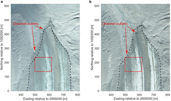
The HGdA is 3.3 km long and extends from 3500 to 2600 m a.s.l., with its terminus located at 45°58′58.366″ N / 7°31′24.979″ E in the summer of 2020. The glacier initially flows from southeast to northwest from the Mont Brûlé, turning to flow from south to north toward the terminus. The subglacial hydrology of the HGdA has been investigated extensively in the scientific literature (e.g. Hubbard and others, Reference Hubbard, Sharp, Willis, Nielsen and Smart1995; Nienow and others, Reference Nienow, Sharp and Willis1996; Nienow and others, Reference Nienow, Sharp and Willis1998; Mair and others, Reference Mair, Nienow, Sharp, Wohlleben and Willis2002a, Reference Mair, Sharp and Willis2002b). For several years, the glacier has had two main subglacial outlet channels, located along the eastern side of the glacier terminus (Fig. 2). More recently, the sediment dynamics have also been studied (Swift and others, Reference Swift, Nienow and Hoey2005; Perolo and others, Reference Perolo2019). The bedrock underlying the glacier is composed of schistose granites, gneiss and metagranitoides (Tranter and others, Reference Tranter2002; Geological Atlas of Switzerland, 2020). This is covered by a layer of sediment, which in most places is several decimeters thick (Mair and others, Reference Mair2003). The ice volume of the HGdA in the year 1999 was estimated to be 0.25 ± 0.07 km3 based on topographic data (Farinotti and others, Reference Farinotti, Huss, Bauder and Funk2009a, Reference Farinotti, Huss, Bauder, Funk and Truffer2009b). By far the biggest part of the glacier volume is located below the equilibrium-line altitude (ELA), meaning that the HGdA is highly sensitive to increases in average air temperature. Indeed, the tongue of the HGdA has retreated by more than 400 m in length over the past 20 years (Gabbud and others, Reference Gabbud, Micheletti and Lane2016) and serves as a proxy for alpine glaciers at medium to low elevations having a proportionately small accumulation area. Such glaciers are expected to continue to retreat rapidly over the next few decades (Salzmann and others, Reference Salzmann, Machguth and Linsbauer2012; Huss and others, Reference Huss, Jouvet, Farinotti and Bauder2010).

Fig. 2. Aerial orthoimagery of the tongue of the Haut Glacier d'Arolla taken in (a) September 2014 and (b) September 2015. The red square indicates the area over which high-density GPR measurements were acquired in August 2015. The GPR survey lines were oriented east–west. The dashed black line represents the most recent GLIMS glacier outline based on satellite imagery from 2015 (Paul and others, Reference Paul2019).
The much-less-studied GdO is 7 km long and extends from 3790 to 2500 m a.s.l., flowing from northeast to southwest from the summit of the Pigne d'Arolla, with its terminus located at 45°56′18.908″ N / 7°25′20.212″ E in the summer of 2020. There are two active tributary glaciers: de Blanchen and du Petit Mont Collon. The bedrock underlying the glacier is composed of a mixture of metagranitoides and metagabbros (Geological Atlas of Switzerland, 2020). Field observations where the glacier has recently receded show that this is typically covered by a thin layer of sediment, having a thickness of between a few centimeters and a few decimeters. The ice volume of the GdO was determined in 2009 to be 1.05 ± 0.08 km3 based on airborne GPR and topographic data (Farinotti and others, Reference Farinotti, Huss, Bauder, Funk and Truffer2009b; Gabbi and others, Reference Gabbi, Farinotti, Bauder and Maurer2012). Since, similar to the HGdA, most of the glacier volume is currently located below the ELA, the GdO is sensitive to increases in average air temperature and has been retreating rapidly at an average rate of 40 m in length per year over the past 60 years (GLAMOS, 1881–2019).
2.2 GPR measurements
Zero-offset, high-density GPR data were acquired on both the HGdA and GdO using a lightweight, real-time-sampling GPR instrument manufactured by Radarteam, Sweden. The single transmitter–receiver antenna employed for the surveys has a nominal center frequency in air of ~70 MHz with a bandwidth between 20 and 140 MHz. To maximize portability, the GPR system was suspended from a backpack with the antenna located 0.4 m above the ground, which was found to provide good antenna coupling and a measurement quality that was virtually the same as that obtained with the antennas located directly on the ice surface. Data were collected on foot following parallel lines that were spaced either 1- or 2-m apart. GPR traces were recorded continuously at a frequency of ~3.5 Hz using a time-sampling interval of 3.125 ns, the latter of which was sufficient to avoid temporal aliasing. The system has a fixed scan time of 1600 ns, which corresponds to a depth of investigation of ~134 m assuming a radar wave speed in glacier ice of 0.167 m ns−1 (Murray and others, Reference Murray, Stuart, Fry, Gamble and Crabtree2000). In the current study we focus on areas where the ice thickness was <60 m.
GPR lines spaced 1-m apart were surveyed over a 120 m × 100 m region of the snout marginal zone of the HGdA in August 2015 (Fig. 2). On the GdO, an ~200 m × 100 m region was surveyed using a 2-m line spacing in August 2017 (Fig. 3). Over the latter period, a 200-m-long GPR line was also repeatedly measured over 24 h (hourly from 7 a.m. to 9 p.m. and every 3 h from 9 p.m. to 6 a.m.) in order to investigate the repeatability of the measurements over the course of a summer day (Fig. 3). Although previous work has suggested that radar velocity, attenuation and reflectivity in porous near-surface ice may vary strongly because of changing water content (Kulessa and others, Reference Kulessa, Booth, Hobbs and Hubbard2008), no significant changes in the positions of the glacier bed or other major reflectors were detected, and relative reflection amplitudes remained stable (Figs S1 and S2 in Supplementary material). The influence of the orientation of the GPR antenna on the detectability of the glacier bed was also studied for the GdO (Langhammer and others, Reference Langhammer, Rabenstein, Bauder and Maurer2017), with results suggesting that GPR survey lines are best run perpendicular to ice flow with the radar antenna oriented perpendicular to the line direction. We adopted the latter strategy when acquiring the GPR data in this study, meaning that the parallel survey lines were oriented east–west at the HGdA, and northwest–southeast at the GdO.

Fig. 3. Drone-based orthoimagery of the tongue of the Otemma glacier taken in (a) August 2017 and (b) August 2018. The red polygon indicates the area over which high-density 3-D GPR measurements were acquired in August 2017. The GPR survey lines were oriented northwest–southeast. The black line indicates the location of the GPR repeat profile analyzed in the Supplementary material (Figs S1 and S2). The red dot displays the location of a moulin. The region not covered by the drone survey is indicated in white. The dashed black line represents the most recent GLIMS glacier outline based on satellite imagery from 2015 (Paul and others, Reference Paul2019).
For the GPR surveys on both the HGdA and the GdO, accurate positioning was achieved along each profile line using real-time dGPS navigation. A dGPS base station was installed at both sites close to the glacier terminus. Two operators were used to collect the GPR data, each of whom carried a dGPS rover antenna. One operator walked ahead and navigated along a pre-programmed path, whereas the other followed with the GPR system. The position of the GPR antenna was logged at a frequency of 10 Hz in order to provide GPS coordinates for each recorded trace with ~±10 cm precision. GPR survey lines were found to deviate from the pre-programmed paths by no more than 25 cm.
2.3 Data processing
Processing of the data from the HGdA and the GdO consisted of an initial series of steps to obtain a migrated 3-D GPR data volume, which was followed by picking and attribute analysis of the reflection from the glacier bed in order to identify subglacial channels. Note that, in general, such channels are not easily seen on the individual GPR profile lines because of the limited vertical resolution of the data. That is, for our 70-MHz antenna with a dominant radar wavelength in ice of over 2 m, it is generally not possible to image separately the channel roofs and floors and thus unambiguously identify these features (Fig S3 in Supplementary material), in particular if the channels are at least partially air-filled. However, as the channels represent a strong contrast in radar reflection coefficient compared to their surroundings, they can be imaged via amplitude analysis along the bed. All processing was done in the MATLAB computing environment using customized codes. Table 1 summarizes the initial steps carried out on the data. During the GPR data acquisition, the dGPS rover antenna logging the GPR instrument position experienced occasional drops in precision leading to local shifts in recorded elevation which had to be manually removed and replaced using linear interpolation. An acquisition pattern adjustment of 0.4 m was also necessary between GPR lines run in opposite directions (i.e. a position shift of 0.2 m in each direction) in order to correct for positioning errors related to system timing delays and the angle of the GPS rover antenna.
Table 1. Initial processing steps applied to the 3-D GPR data

Figure 4 shows the results of applying the processing steps described in Table 1 to a single east–west GPR survey line from the HGdA dataset collected along 1 092 150-m northing. In Figure 4a, we see that the GPS-corrected and binned raw data do not allow for easy identification of subglacial structure due to the presence of: (i) the emitted GPR pulse; (ii) unwanted low frequencies (‘wow’) upon which the GPR reflections are superimposed and (iii) amplitude variations due to signal attenuation and differences in antenna coupling. After amplitude normalization, removal of the emitted pulse, dewow, gain and time interpolation (Fig. 4b), the data become easier to interpret but are still contaminated by numerous hyperbolic diffraction events related to the presence of small scatterers (water pockets, air voids and boulders) within the ice. Figure 4c shows the result of 3-D topographic time migration using the algorithm of Allroggen and others (Reference Allroggen, Tronicke, Delock and Böniger2015) with a migration aperture of 10 m and assuming a constant radar wave velocity of 0.16 m ns−1. The latter value was found to provide the best collapse of diffraction hyperboloids in the 3-D volume and is appropriate for temperate ice (Plewes and Hubbard, Reference Plewes and Hubbard2001; Murray and others, Reference Murray, Booth and Rippin2007). Finally, Figure 4d shows the final GPR image after time-to-depth conversion and topographic correction, where we see in blue and red the glacier surface topography and position of the bed, respectively.

Fig. 4. Demonstration of the GPR processing described in Table 1 for one east–west survey line from the HGdA acquired along 1 092 150 m northing: (a) binned and time-zero-corrected raw data (steps 1–4); (b) after trace normalization, direct arrival removal, dewow, gain and trace interpolation (steps 5–9); (c) after subsequent 3-D topographic Kirchhoff time migration (step 10) and (d) after time-to-depth conversion and correcting for topography (steps 11 and 12). The blue line shows the ice surface whereas the red line indicates the picked glacier bed reflection.
After the initial processing described above, the migrated 3-D GPR image was analyzed to quantify the amplitude characteristics of the reflection along the glacier bed. Subglacial channel locations are expected to correspond with anomalously high bed reflection amplitudes because they represent a strong contrast in dielectric permittivity (e.g. ice/air or ice/water) compared to their surroundings (e.g. ice/bedrock) (Wilson and others, Reference Wilson, Flowers and Mingo2014; Church and others, Reference Church2019). To this end, we first performed a manual line-by-line picking of the glacier bed reflection (Fig. 4d), the results of which were used to fit a thin plate smoothing spline to the glacier bed surface. For the HGdA, the mean deviation between this modeled surface and the glacier-bed picks was 0.27 m. For the GdO, it was 0.39 m. Next, the 3-D GPR image was ‘flattened’ along the modeled bed surface by applying a linear Fourier phase shift to each trace, the latter of which allowed us to conform the data smoothly to the picked bed topography. Although not essential for the amplitude analysis described below, flattening the data in this manner greatly facilitated the extraction of bed reflection profiles, in the sense that they could be obtained by slicing horizontally through the 3-D data matrix. Next, we calculated the magnitude of the Hilbert transform of each trace (i.e. the so-called ‘instantaneous amplitude’), which provides the trace amplitude envelope and is commonly used in seismic data processing to quantify reflection strength (e.g. Taner and others, Reference Taner, Koehler and Sheriff1979). Finally, the maximum of this result was computed over a small (2-m) window containing the bed reflection in order to compensate for any errors in our determination of the precise location of the bed. The resulting 2-D map of maximum reflection strength along the glacier bed can be examined for spatial patterns indicative of subglacial channels.
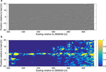
In Figure 5, we show the application of our amplitude processing to the single GPR profile from the HGdA dataset presented in Figure 4. Figure 5a shows the GPR image from Figure 4d after flattening the data to the picked glacier bed surface. In Figure 5b, we plot the absolute value of the Hilbert transform, where a strong increase in reflection strength around the location of the bed can be seen. Note, however, that the distribution of amplitudes along the bed is highly non-uniform due to the variability in reflectivity at this interface. An image plot of the maximum instantaneous amplitude over a small window containing the bed reflection, for all of the survey lines in the 3-D dataset, is used to identify coherent trends related to the presence of subglacial channels. These latter results are presented and described in Sections 3.1 and 3.2 for the HGdA and GdO datasets, respectively.

Fig. 5. Illustration of our amplitude analysis of the glacier bed reflection: (a) processed GPR survey line from Figure 4d ‘flattened’ to the bed reflection event and (b) corresponding normalized absolute value of the Hilbert transform along each trace, which quantifies reflection strength.
2.4 Validation of results
The results of our analysis were assessed using two different strategies. The first one involved comparison with aerial orthoimagery acquired at some time after the GPR surveys, where it was possible to either see directly the investigated subglacial channels, or evidence thereof, due to glacier retreat and ice-marginal breakup. At the HGdA, although glacier retreat between 2014 and 2015 was rapid (30 m in length), it was not enough to reveal directly the channels identified with GPR. However, we could compare our results with the location of subglacial channels exiting the glacier snout in 2014 and 2015. Ortho-rectified aerial imagery acquired by Flotron SA in two consecutive years (September 2014 and September 2015) also indicated the development of two large fractures on the HGdA surface within 1 month of our GPR survey. These were later verified in the field to be places where the ice ruptured, which we believe occurred due to instabilities related to surface melting and the enlargement of marginal subglacial channels below. At the GdO, drone imagery was acquired in August 2017 and August 2018 using DJI Phantom 3 and Phantom 4 drones, respectively. The corresponding orthoimages documented the collapse of a large portion of the main outlet channel in the summer of 2018 along with rapid glacier retreat, which provided direct validation of the GPR findings ~1 year after the measurements.
As a second validation method, we estimated the hydraulic potential at the glacier bed (Shreve, Reference Shreve1972) in order to predict the theoretically most likely trajectories of subglacial channels. This was done by summing contributions to the potential related to elevation and ice overburden pressure as follows:

where φ is the hydraulic potential, ρ w = 1000 kg m−3 is the density of water, g = 9.81 m s−2 is the acceleration of gravity, z is the glacier bed elevation, ρ i = 910 kg m−3 is the density of ice, H is the ice surface elevation and c is a constant that accounts for the degree of pressurization of the channels. A value of c = 0 represents unpressurized flow, whereas a value of c = 1 represents fully pressurized flow where the ice overburden pressure significantly influences the hydraulic gradient and thereby the flow paths. Ice surface topography data for the HGdA and GdO were obtained from the SwissAlti3D Digital Elevation Model for the summers of 2012 and 2009, respectively (SwissTopo, 2020). These data have horizontal and vertical resolutions of 2 m and were derived from aerial imagery. Glacier bed elevations for the HGdA at 20-m horizontal resolution, derived from irregularly spaced GPR surveys, were supplied by Dr Ian Willis at the University of Cambridge (Sharp and others, Reference Sharp1993). For the GdO, bed elevations at 50-m horizontal resolution were obtained from Dr Mauro Werder at ETH Zurich and derived from helicopter-borne GPR surveys conducted in 2009 (Gabbi and others, Reference Gabbi, Farinotti, Bauder and Maurer2012). Considerations by Hooke (Reference Hooke1984) show that, given high enough discharge and bed slope, especially when ice thicknesses are small (i.e. <50 m), the flow in subglacial channels may not be pressurized. It is also unlikely that such channels close during winter due to insufficient ice overburden weight. Channel positions, however, may be inherited from when they formed under deeper ice in pressurized conditions. As these aspects remain uncertain, we apply Eqn (1) using values of c = 0, c = 0.5 and c = 1 in our analysis.
The gradient of the Shreve potential yields the local flow direction, which is used to compute flow accumulation and estimate the most likely subglacial flow pathways. The latter was done using the Topotoolbox package in MATLAB (Schwanghart and others, Reference Schwanghart, Groom, Kuhn and Heckrath2013; Schwanghart and Scherler, Reference Schwanghart and Scherler2014). To form a channel feature, flow accumulation thresholds of 180 upstream cells for the HGdA (cell size 20 m × 20 m) and 60 upstream cells for the GdO (cell size 50 m × 50 m) were considered. These values are different for each glacier because of the different sizes of the bed topography grid cells in each case; a lower number of larger cells is needed to achieve the same amount of flow as when using smaller cells. Note that the computed channel features reflect the hydraulic conditions according to the Shreve potential at the times when the SwissAlti3D DEMs for each glacier were acquired, which are not the same as the acquisition dates of the GPR datasets. However, given the fact that neither the overall surface topography nor the contributing areas of each glacier changed substantially between the DEM and GPR acquisitions, we do not expect a significant change in the predicted subglacial channel locations. Therefore, the considered DEM and bed topography datasets and resulting Shreve calculations provide the best available theoretical insight into the hydraulic potential underneath the two glacier tongues for comparison with our GPR data.
3 Results
3.1 Haut glacier d'Arolla
In Figure 6, we present the results of our analysis of the HGdA GPR dataset. Figure 6a shows the measured ice surface topography over the GPR survey region. The local slope of the glacier surface can be seen to be approximately constant and is oriented toward the northwest. In Figure 6b, we plot the GPR-derived glacier bed topography. Unlike the ice surface topography, the glacier bed is seen to slope toward the north in the western half of the profile and toward the northeast in the eastern half of the profile, with a faint rise separating these two regions. Figure 6c shows the calculated ice thickness over the survey region, which was obtained by subtracting the elevations in Figure 6b from those in Figure 6a.

Fig. 6. GPR data analysis results for the HGdA site: (a) glacier surface elevation (m a.s.l.); (b) glacier bed elevation (m a.s.l.); (c) ice thickness (m); (d) maximum normalized reflection strength along the glacier bed; (e) zoom of September 2014 orthophoto from Figure 2a and (f) zoom of September 2015 orthophoto from Figure 2b.
Here, we observe that the ice thickness decreases both in the direction of the glacier terminus toward the north, as well as strongly toward the western edge of the glacier where thinning is more significant. The eastern part of the zone of interest has more bare ice whose higher albedo leads to less melting in this region. Further east outside of the GPR survey region, a morainic debris cover of up to several decimeters thick reduces melting due to insulation (Fig. 2b).
Figure 6d shows the maximum absolute value of the Hilbert transform of the GPR data in the location of the glacier bed for the HGdA dataset, which again quantifies the reflection strength. In this image, higher values are expected to correspond with the location of subglacial channels due to a stronger contrast in dielectric permittivity. We see in the figure that there are two main zones where the amplitude increases significantly; one with small bends on the western side of the survey grid and another primarily linear zone on the eastern side. Both of these zones are oriented approximately north–south and measure several meters in width. The fact that they show continuity perpendicular to the direction of the GPR survey lines (which were run east–west) suggests that they are not artifacts of the data acquisition or processing, but rather represent real differences in GPR bed reflectivity. The western-most zone ends at the glacier terminus at a channel outlet (Fig. 2) and is aligned with the topographic gradient of the bedrock topography (Fig. 6b). It is situated in a region of shallow ice having a thickness of <15 m. The zone on the eastern side, on the other hand, is located in region having ice thickness between 20 and 35 m. It is wider and appears to be associated with a higher bed reflectivity, and may represent a subglacial channel that continues toward the northeast, ending at the second, eastern channel outlet (Fig. 2). Both zones are separated by the rise in bed topography near the center of the glacier tongue (Fig. 6b).
Figures 6e and 6f show zooms of the orthoimages from Figures 2a and 2b over the GPR survey region, respectively. The image in Figure 6e was acquired in September 2014, and reflects quite well the conditions of the glacier surface when the GPR data were acquired in August 2015, aside from some recession near the glacier terminus. The image in Figure 6f, on the other hand, was acquired in September 2015 ~1 month after the GPR acquisition. Here, we see that two notable fractures have developed on the glacier surface in the western and eastern parts of the survey region, which were not present during the GPR survey. A subsequent visit to the HGdA in October 2015 confirmed that the ice ruptured in these locations and that the fractures continued all the way to the glacier bed, where the sound of rushing water could be heard. With regard to the western-most fracture, we observe that its overall trend is remarkably similar to that of the western zone of increased reflection amplitude in Figure 6d. This suggests that the fracture represents the beginning of the collapse of unstable ice over a shallow subglacial channel, and that the GPR survey allowed for detection of this channel before the fracturing occurred. With regard to the eastern-most fracture, we see that it loosely corresponds to a region of high reflectivity in roughly the same location (Fig. 6d), which suggests that it may represent a small branch of the larger eastern-most subglacial channel that has ruptured to the surface.
Figure 7 shows the results of our Shreve hydraulic potential analysis for the HGdA site, which was performed over a broad region encompassing the entire glacier tongue (Fig. 7a). In Figure 7b we plot the Shreve potential computed for c = 0 in Eqn (1), which corresponds to the case of unpressurized (open-channel) flow. The main drainage pathways obtained via flow accumulation, as well as the suspected channel locations digitized from the GPR results in Figure 6d, are shown as red and yellow lines, respectively. Similarly, Figures 7c and 7d plot the results obtained for values of c = 0.5 (partially pressurized flow) and c = 1 (fully pressurized flow). We observe that the GPR-derived channel locations correspond well with the Shreve hydraulic potential scenarios for unpressurized and partly pressurized flow, although the best correspondence would result from a combination of these two scenarios. The location of the western channel also corresponds to the Shreve hydraulic potential for fully pressurized flow. In the location of the GPR survey, the glacier ice was relatively shallow with a maximum thickness of 45 m, which suggests that pressurized flow there is unlikely. Further upstream, however, the flow may be (or have been) pressurized several years ago due to greater ice thicknesses, which may have established the channels in their present positions (Sharp and others, Reference Sharp1993), explaining the current location of channels further downstream. Also note that the Shreve potential was computed based on glacier surface elevation data from 2012, whereas the GPR data were recorded in 2015, which may account for some of the differences between the two results.

Fig. 7. (a) Zoom of September 2015 orthophoto from Figure 2b in the region of the tongue of the HGdA, upon which the GPR amplitude analysis results from Figure 6d are superposed; (b–d) calculated Shreve hydraulic potential along with the theoretically most likely flow paths (red lines) and the manually digitized GPR-derived subglacial channel positions (yellow lines). The Shreve hydraulic potential is presented for (b) open-channel flow (c = 0); (c) partly pressurized flow (c = 0.5) and (d) fully pressurized flow (c = 1). The dashed black line represents the GLIMS glacier outline for the summer of 2015 (Paul and others, Reference Paul2019).
3.2 Glacier d'Otemma
In Figure 8, we present the results of our analysis of the GdO GPR dataset. Figures 8a, 8b and 8c show the measured ice surface topography, GPR-derived glacier bed elevations and calculated ice thickness over the survey region, respectively. All of these are superposed on a drone orthophoto from August 2018. We see in the figure that the local surface topography slopes uniformly toward the glacier terminus, but on the lower part of this slope there is a slight surface depression which was developing into a channel collapse at the time of the GPR survey. Compared to the HGdA, the bed topography at the GdO is relatively flat over most of the survey region, with the exception of a ~3-m-deep depression toward the northeast. Toward the southern edge of the survey area, there are strong increases in the elevation of both the glacier bed and the ice surface, which are related to the valley's U-shape and reduced melting in this location due to the large amount of debris cover. The ice thickness is seen to follow the commonly observed pattern of decreasing toward the glacier terminus, and is roughly constant across the glacier width with the exception of the zone near the terminus associated with the developing channel collapse.

Fig. 8. GPR data analysis results for the GdO site: (a) glacier surface elevation (m a.s.l.); (b) glacier bed elevation (m a.s.l.); (c) ice thickness (m); (d) maximum normalized reflection strength along the glacier bed; (e) zoom of August 2017 orthophoto from Figure 3a and (f) zoom of August 2018 orthophoto from Figure 3b.
Figure 8d shows the maximum absolute value of the Hilbert transform of the GPR data in the location of the glacier bed for the GdO dataset. In contrast to the HGdA, we see that there is a single clear zone showing a strong increase in reflection strength that extends across the entire GPR survey region. This zone, which we believe represents a large subglacial channel, appears to be up to 10 m in width. It originates in the east near the center of the glacier, makes a turn toward the northern boundary of the survey region, and then continues along the northern glacier margin before making a relatively sharp turn back toward the center of the glacier. The latter trajectory appears logical in the sense that it tends to avoid the higher areas of the bedrock topography (Fig. 8b). Similar to the HGdA, the fact that the high-amplitude region shows continuity perpendicular to the direction of the GPR survey lines (which were run roughly south–north) indicates that it is not an artifact of the data acquisition or processing, but rather reflects real differences in bed reflectivity.
Figures 8e and 8f show zooms of the orthophotos presented in Figures 3a and 3b, respectively. The image in Figure 8e was acquired in August 2017 during the acquisition of the GPR data, whereas the image in Figure 8f was acquired ~1 year later. Between these acquisition dates, the GdO retreated by ~40 m on its northern side. A large portion of the region surveyed in 2017 also collapsed sometime between mid-July 2018 and early August 2018, revealing a cavity ~60-m long, 20-m wide and 10-m deep. The position of this cavity coincides well with the suspected subglacial channel location from Figure 8d, and we believe that surface downwasting combined with channel melting from the inside led to the ice becoming unstable. We also see in Figure 8f that the channel enters from the northeast into the collapsed area and continues toward the south before turning westward out of the collapsed area, which is consistent with the GPR results in Figure 8d. Note that collapse of the channel roof during the autumn of 2018 was observed in the field and confirms the channel outflow and inflow positions downstream and upstream of the collapsed section in Figure 8f, respectively. Finally, a moulin was detected further upstream of the main channel (Fig. 3), whose location may provide further validation for the location of the subglacial channel.
Figure 9 shows the results of our Shreve hydraulic potential analysis for the GdO site, which, like the HGdA, was performed over a broad region encompassing the entire glacier tongue (Fig. 9a). Figures 9b, 9c and 9d show the hydraulic potential calculated for c values of 0, 0.5 and 1, respectively. The main drainage pathways obtained via flow accumulation, as well as the suspected channel location digitized from the GPR results in Figure 8d, are again shown as red and yellow lines, respectively. We see that the three flow scenarios lead to reasonably similar drainage patterns that correspond quite well with the GPR results, except for the fact that they do not predict the meandering shape of the identified channel. This may be a result of the significantly lower (50-m) resolution bed topography measurements used for the generation of the Shreve hydraulic potential maps in this case. Indeed, we believe that the meandering shape of the subglacial channel identified in the GPR results reflects strong bedrock control on flow at the GdO via local changes in bed topography and roughness (Alley, Reference Alley1992; Gulley and others, Reference Gulley2014).

Fig. 9. (a) August 2018 orthophoto from Figure 3b overlain on a 2019 satellite image in the region of the tongue of the GdO, upon which the GPR amplitude analysis results from Figure 8d are superposed; (b–d) calculated Shreve hydraulic potential along with the theoretically most likely flow paths (red lines) and the manually digitized GPR-derived subglacial channel position (yellow lines). The Shreve hydraulic potential is presented for (b) open-channel flow (c = 0); (c) partly pressurized flow (c = 0.5) and (d) fully pressurized flow (c = 1). The dashed black line represents the GLIMS glacier outline for the summer of 2015 (Paul and others, Reference Paul2019).
4 Discussion
4.1 Substantive findings
Marginal subglacial channels at the HGdA and GdO were mapped via amplitude analysis of the glacier bed reflection identified in high-resolution 3-D GPR data. The corresponding results were validated using aerial orthoimagery acquired after the GPR surveys, as well as calculation and analysis of the Shreve hydraulic potential. In the case of the HGdA, two subglacial channels were identified; a slightly tortuous one on the western side of the glacier tongue, and a second larger and more linear channel on the eastern side (Fig. 6d). At the GdO, one main, tortuous channel was detected (Fig. 8d), which follows the northern edge of the glacier tongue before turning toward the center of the glacier.
The locations of en- and subglacial channels within temperate alpine glaciers have been previously identified with GPR measurements. However, existing data were generally not acquired at high enough density for processing and analysis in 3-D, which here allows for the mapping of subglacial channels continuously with meter-scale resolution. Indeed, past research has largely involved channel detection along 2-D GPR survey lines and subsequent interpolation of flow pathways when multiple line data were available (e.g. Bælum and Benn, Reference Bælum and Benn2011; Temminghoff and others, Reference Temminghoff, Benn, Gulley and Sevestre2019). Our study, in contrast, focuses on analysis of the amplitude characteristics of the glacier bed reflection in order to create a detailed map of the suspected channel pathways. This also has the advantage of being able to detect channels that may not be easily seen as distinct reflections on individual GPR profiles. Although the acquisition of such high-density GPR data for 3-D analysis is highly laborious, in particular with regard to surveying areas much larger than those considered here on foot, recent technological developments in lightweight, real-time-sampling GPR instruments and drone-based sensing provide promise for carrying out such surveys over larger regions in an automated manner.
The western marginal subglacial channel detected beneath the HGdA (Fig. 6d) corresponds well with the position of a western channel outlet visible on the aerial orthoimages from both 2014 and 2015 (Fig. 2), whereas the wider eastern channel appears to lead toward an eastern channel outlet. Previous subglacial hydrological studies noted two main flow pathways in this area of the HGdA glacier tongue (Sharp and others, Reference Sharp1993). Perhaps most importantly, fractures appearing on the glacier surface ~1 month after the GPR data acquisition (Fig. 6f) follow closely the western subglacial channel trajectory identified in the GPR data. These fractures were later verified in the field and are likely to be the result of ice weakening in the marginal zone due to surface downwasting combined with channel melting.
In contrast to the eastern channel location, the western channel location at the HGdA was found to agree with the Shreve hydraulic potential results for fully pressurized and partially pressurized flow (c = 1, Fig. 7d; c = 0.5, Fig. 7c). Based on this result, it may be possible that the marginal channel positions are inherited from when the ice was thicker and flow conditions were predominantly pressurized. Once established and eroded into the sediment and bedrock, they could only migrate a small amount during the relatively short summer season. In winter, creep closure due to ice overburden pressure would not be strong enough to close the pre-existing channels entirely as the ice is too thin in this zone. Calculation using Glen's flow law (Glen, Reference Glen1958; Hooke, Reference Hooke1984) for an ice thickness of 45 m and a subglacial channel diameter of 4 m yields a channel closure rate of 1.2 m per year meaning that, assuming an 8-month-long winter season, channels would close only by up to one-fifth of their total estimated height.
The detected approximate channel planform geometry at the GdO is different from that at the HGdA in that the channel is more tortuous and resembles a meandering river (Fig. 8d). It eventually reaches a principal outlet at the glacier terminus, which is not directly visible in the orthoimage in Figure 3b but was verified in the field in the autumn of 2018. The channel position was also confirmed by aerial imagery acquired in 2017 and 2018 (Figs 8e and 8f), which document the progressive collapse of the glacier at the precise location where the channel was identified using GPR. The fact that the detected channel roughly coincides with the drainage pathway determined from the Shreve potential calculations, but deviates from the main pathway in a large meandering turn, suggests that local bedrock topography and sediment dynamics may be important factors controlling its course, rather than ice overburden pressure as suggested by Shreve (Reference Shreve1972) and the simplest form of the theory of Röthlisberger (Reference Röthlisberger1972).
Both the HGdA and GdO were found to have similar ice thicknesses at their glacier tongues (Figs 6c and 8c), and are underlain by similar types of bedrocks. However, their glacier bed compositions differ. At the GdO, field observations indicate that the glacier bed consists of uneven bedrock partly covered by a thin sediment layer (i.e. hummocky terrain) whereas at the HGdA it consists of bedrock covered by a thicker and more even sediment layer (Fischer and Hubbard, Reference Fischer and Hubbard1999). This leads to a more uniform glacier bed topography at the HGdA and to less tortuous subglacial channel planforms.
Both the cracks in the ice above the identified subglacial channels at the HGdA, visible on the aerial photo of September 2015 (Fig. 6f), and the channel breakdown at the GdO, shown on the orthophoto of August 2018 (Fig. 8f) point to a potentially important mechanism that has been rarely documented. It appears that temperate alpine glaciers in a rapidly warming climate are not only losing mass due to melting at the surface and via basal melting, but also due to the removal of large volumes of ice via the collapse and disintegration of subglacial channels. Subglacial channel collapse has indeed been observed in a small number of other studies (Konrad, Reference Konrad1998; Bartholomaus and others, Reference Bartholomaus, Anderson and Anderson2011; Stocker-Waldhuber and others, Reference Stocker-Waldhuber, Fischer, Keller, Morche and Kuhn2017), and the research presented here leads us to the hypothesis that the collapse is related to a situation where surface melt reduces ice thickness at the snout margin and thereby also the extent of winter closure of the subglacial channel. Continued surface melt eventually leads to structural weaknesses in the ice and collapse. If this hypothesis can be confirmed with a detailed analysis of surface displacement and melt, it would corroborate the findings of the above studies, as well as suggest that the effects of subglacial channel collapse may be more important for rapid glacier retreat on a global scale than previously assumed.
Our results for the HGdA and GdO show that 3-D analysis of high-resolution, densely acquired GPR data is useful for detecting channel planforms underneath temperate alpine glaciers. Such channel planforms are important for understanding the role that snout marginal channels play in the export of sediment. Depending on the channel geometry and glacier bed topography, the shear stress distribution at the glacier bed varies and this in turn will influence the sediment transport capacity of the conduit (Chen and others, Reference Chen, Liu, Gulley and Mankoff2018; Perolo and others, Reference Perolo2019). With future glacier retreat and thinning, the subglacial drainage networks underneath the HGdA and the GdO are likely to extend further up-glacier due to an upward shift of the ELA, leading to more meltwater input at higher elevations (Nienow and others, Reference Nienow, Sharp and Willis1998; Beaud and others, Reference Beaud, Flowers and Venditti2018). The drainage networks will thereby access new sediment sources underneath the glaciers (Nienow and others, Reference Nienow, Sharp and Willis1998; Swift and others, Reference Swift, Nienow and Hoey2005; Gulley and others, Reference Gulley2012a), leading to changes in sediment fluxes further downstream.
4.2 Methodological challenges
Reliable identification of the glacier bed reflection is critical for the successful detection of subglacial channels using the methodology described in this paper. In this regard, a number of factors can affect the quality and interpretability of this reflection. First, englacial scattering due to inclusions of water or voids in temperate ice may strongly attenuate the GPR signal, thereby reducing the radar energy reaching the bed as well as adding significant complexity to the corresponding data (Plewes and Hubbard, Reference Plewes and Hubbard2001; Fig. 4b). Second, the combination of GPR antenna radiation pattern, survey line orientation, and underlying bedrock topography may lead to poor visibility and detection of the glacier bed in some cases (Moran and others, Reference Moran, Greenfield and Arcone2003; Rutishauser and others, Reference Rutishauser, Maurer and Bauder2016; Langhammer and others, Reference Langhammer, Rabenstein, Bauder and Maurer2017). Finally, internal layering of the glacier ice, including sediment layers, may complicate the interpretation of the GPR data because layering close to the glacier bed may be difficult to distinguish from the bed reflection (Lapazaran and others, Reference Lapazaran, Otero, Martín-Español and Navarro2016). Despite these challenges, we found that we were able to easily identify the glacier bed in both the HGdA and GdO datasets along most of our survey lines. Indeed, GPR measurements made using the same real-time-sampling instrument much higher up on the HGdA (data not shown) indicated that identification of the bed reflection was even possible where the ice thickness was on the order of 100 m. Note that, in instances where identification of the bed reflection was difficult, analysis of the 3-D GPR datasets in both the survey in-line and cross-line directions proved to be helpful.
Another important consideration for the success of the methodology presented in this paper is the reliability of the amplitude information extracted at the glacier bed. A number of factors can influence the spatial pattern of such amplitudes, which include the quality of the data migration as well as spatial variations in englacial attenuation and scattering that are not taken into account when using a standard, spatially invariant gain function. Furthermore, even in a best-case scenario where the data have been perfectly migrated and attenuation and scattering in the ice have been perfectly compensated, the horizontal resolution of the GPR image at the glacier bed will still be on the order of the dominant wavelength of the GPR pulse (e.g. Stolt and Benson, Reference Stolt and Benson1986), which for our 70-MHz system is ~2 m. This means that, at the very least, the images of bed reflection amplitude obtained from the GPR data will represent laterally smeared versions of reality, and that the results presented in Figures 6d and 8d must therefore be considered as noisy, low-pass-filtered versions of the true bed reflectivity distribution. Nevertheless, the research presented in this paper demonstrates that such GPR-derived amplitude maps can still offer clear and insightful information regarding the location of subglacial channels. Indeed, the uncertainties that we observed through our repeat-line analysis at the GdO (Figs S1 and S2 in Supplementary material) showed that variations in the recovered amplitudes along the line with time were significantly less than those associated with the presence of subglacial channels.
A further factor influencing the accuracy of our processed GPR images is spatial variability in the subsurface radar wave velocity, the latter of which we assumed to be equal to a constant value of 0.16 m ns−1 in our analysis. Because of the common-offset nature of the acquired data, more detailed velocity information was not available and the selected value, which is consistent with other velocities published for temperate ice (Plewes and Hubbard, Reference Plewes and Hubbard2001; Murray and others, Reference Murray, Booth and Rippin2007), tended to provide the best collapse of diffraction hyperboloids. As a result, errors may exist in the identified location of the glacier bed due to localized velocity variations caused by zones of increased ice water content and the presence of water- and air-filled channels. Nevertheless, these types of errors do not impact the determined planform geometry of the subglacial channels because reflection amplitudes are analyzed along the manually picked glacier-bed reflection.
Finally, despite the fact that we have considered 3-D GPR datasets consisting of densely spaced parallel survey lines in this study, a strong spatial sampling bias exists in these data in the sense that the line spacing (1 m for the HGdA and 2 m for the GdO) is significantly greater than the spacing of measurements along the lines (~0.2 m for both datasets). Consequently, migration will not perfectly collapse hyperboloids into points and artifacts may exist in the processed data (Grasmueck and others, Reference Grasmueck, Weger and Horstmeyer2005). Close examination of GPR profiles before and after migration (Fig. 4) was performed in order to check for major artifacts that may have significantly altered our results. In future studies, the line spacing for such 3-D analyses should be kept as small as possible (ideally 0.5–1.0 m), although the corresponding surveys would become extremely laborious for regions larger than those considered here. One potential solution is to perform the GPR work via drone, following a precise grid with dGPS navigation and maintaining a minimum distance from the glacier surface.
5 Conclusions
The use of densely spaced survey lines in conjunction with dGPS navigation enabled us to record high-resolution 3-D GPR datasets in the snout marginal zones of two alpine glaciers. Amplitude analysis of the GPR reflection along the glacier bed made it possible to reveal areas with a significant change in bed reflectivity, which allows for the identification of subglacial channels that may otherwise be difficult to detect on individual GPR profiles.
The subglacial channels detected at the HGdA and GdO sites measure several meters in width but exhibit different planform geometries. The two channels observed at the HGdA are only slightly meandering, whereas the channel detected at the GdO meanders strongly. We suspect that this difference is a result of differences in glacier bed topography, with the GdO bed being composed of bedrock outcrops and a thin sediment layer, and the HGdA bed being overlain by a thicker sediment layer and presenting a more uniform topography.
Assessment of aerial imagery acquired before and after the GPR surveys, as well as computation and analysis of the Shreve hydraulic potential, allowed us to validate the channel positions identified in the GPR results. The occurrence of cracks at the glacier surface at the HGdA and the collapse of a subglacial channel at the GdO coincide perfectly with the GPR-derived channel positions. The principal flowpaths computed from the Shreve potential closely match these channel positions, despite the relatively coarse grid size available for the Shreve analysis.
The results presented in this paper show the potential for 3-D analysis of high-density GPR data acquired on temperate alpine glaciers to provide detailed information about subglacial hydrology. Future drone-supported GPR surveys with a larger spatial extent may yield valuable knowledge about en- and subglacial channel pathways, possibly in 3-D, underneath rapidly retreating alpine glaciers. This information is critical for better understanding of the drainage pathways, hydraulic properties and sediment export potential of such channels as glaciers retreat and new sediment sources at the glacier bed become accessible due to upstream extension of the subglacial drainage network. With further atmospheric warming, the disintegration and collapse of subglacial channels may become an even more important mechanism contributing to the rapid retreat of temperate alpine glaciers in the near future.
Supplementary material
The supplementary material for this article can be found at https://doi.org/10.1017/jog.2021.26
Acknowledgements
We thank Ludovic Baron for help with development of the GPR acquisition system and fieldwork at the HGdA, as well as Boris Ouvry and Martino Sala for help with fieldwork at the GdO. GPR-derived bed topography data for the HGdA were provided by Ian Willis at the University of Cambridge. GPR-derived bed topography data for the GdO were provided by Mauro Werder at ETH Zurich. This research was supported by the University of Lausanne and the Canton de Vaud, Switzerland. Two anonymous reviewers and Editor Dustin Schroeder provided very valuable comments on a previous version of this manuscript.


 Open access