


1. Introduction
The current evidence of a warming climate, expected to have greatest impacts in the high northern latitudes, may increase Greenland ice-sheet surface melting and dynamic losses with associated contributions to sea-level rise (Reference WalshWalsh and others, 2005; Reference Meehl and SolomonMeehl and others, 2007) up to an increase of 0.1–0.5 m possible by 2100 (Reference Pfeffer, Harper and O’NeelPfeffer and others, 2008). Recent studies show an increasingly negative mass balance (Reference ZwallyZwally and others, 2005; Reference BoxBox and others, 2006; Reference LuthckeLuthcke and others, 2006; Reference Rignot, Box, Burgess and HannaRignot and others, 2008) observed from both inland and outlet glacier thinning (Reference AbdalatiAbdalati and others, 2001; Reference Rignot and ThomasRignot and Thomas, 2002; Reference KrabillKrabill and others, 2004; Reference Howat, Joughin, Fahnestock, Smith and ScambosHowat and others, 2008b) and accelerating ice flows along the margins of the ice sheet (Reference Rignot and KanagaratnamRignot and Kanagaratnam, 2006; Reference Howat, Joughin and ScambosHowat and others, 2007). In addition, remote-sensing observations of the ice-sheet surface are widely used to assess melt extent and timing with passive microwave, thermal and scatterometer satellite data and show melt increases over recent decades (Reference Abdalati and SteffenAbdalati and Steffen, 1997; Reference Smith, Sheng, Forster, Steffen, Frey and AlsdorfSmith and others, 2003; Reference MoteMote, 2007; Reference TedescoTedesco, 2007; Reference Hall, Williams, Luthcke and DigirolamoHall and others, 2008). A study has also identified that enhanced melting on the ice sheet may be partly driven by Arctic sea-ice retreat (Reference Rennermalm, Smith, Stroeve and ChuRennermalm and others, 2009). Glacier dynamics may be affected by meltwater reaching the bedrock from surface melt or supraglacial lake drainages (Reference Lüthje, Pedersen, Reeh and GreuellLüthje and others, 2006; Reference Box and SkiBox and Ski, 2007; Reference DasDas and others, 2008), lubricating the ice–bedrock interface to accelerate velocities of outlet glaciers (Reference Zwally, Abdalati, Herring, Larson, Saba and SteffenZwally and others, 2002; Reference McMillan, Nienow, Shepherd, Benham and SoleMcMillan and others, 2007) and by basal melting influencing the buttressing effect of floating glacial tongues (Reference Thomas, Abdalati, Frederick, Krabill, Manizade and SteffenThomas and others, 2003). At least two studies have since confirmed a link between surface melt and ice-sliding velocity, especially in late summer and on the ice sheet proper rather than in outlet glaciers (Reference JoughinJoughin and others, 2008a; Reference Shepherd, Hubbard, Nienow, McMillan and JoughinShepherd and others, 2009). However, it remains poorly understood whether the generated meltwater leaves the ice sheet quickly via moulins, disperses englacially or even refreezes within the ice sheet without exiting. A prime reason for this is a lack of hydrologic measurements of meltwater leaving the ice sheet and entering the ocean. As remote-sensing platforms capable of monitoring river and lake fluctuations are still in their infancy (Reference Alsdorf, Rodríguez and LettenmaierAlsdorf and others, 2007) and direct river discharge measurements are rare (e.g. Reference Mernild, Hasholt, Kane and TidwellMernild and others, 2008), alternative methods of observing meltwater losses to the ocean are needed.
Here we explore using remotely sensed extent and concentration of suspended sediments in the Kangerlussuaq estuary, downstream from the Russell Glacier catchment and several other outlet glaciers of the Greenland ice sheet, as a proxy for ice-sheet meltwater discharge. This estuary is fed by two major glacier-fed rivers draining a large area of the ice sheet. River runoff forms a visible and buoyant surface plume, rich in suspended sediments, upon entering the denser marine water.
The linkage between terrestrial hydrology and estuary plumes has been investigated elsewhere using satellites, but not in Greenland. Visible/near-infrared remote sensing has a long history of quantifying water quality in both terrestrial and coastal waters by developing empirical algorithms describingthe relationships between remotely sensed reflectance and in situ data, including suspended sediment concentration (SSC) (Reference Ritchie, Cooper and SchiebeRitchie and others, 1990; Reference Chen, Curran and HansomChen and others, 1992; Reference Doxaran, Froidefond, Lavender and CastaingDoxaran and others, 2002; Reference Miller and McKeeMiller and McKee; 2004). Although various algorithms and spectral bands are used to calibrate the satellite imagery, each site-specific study has shown successful quantification of SSC. While SSC is a traditional measure of estuary suspended sediment and is related to discharge, plume area is also found to be a robust indicator of discharge (Reference Halverson and PawlowiczHalverson and Pawlowicz, 2008). For Greenland, we propose that plume development is driven by hydrologic outputs from the ice sheet, as driven by surface-melt extent and supraglacial lake outburst drainage events.
Here we ask: Can estuary sediment plumes be detected remotely using MODIS satellite imagery? Does overall developed plume size reflect year-to-year variations in total ice-sheet surface melting? How important are short-term hydrologic events (e.g. intense melt episodes and supraglacial lake drainages) to plume dynamics? We hypothesize that increased meltwater outputs from the ice sheet will register in the downstream estuary as an increase in plume area or reflectivity, SSC, or both, thus enabling sediment plumes to be exploited as a proxy for ice-sheet meltwater discharge to the ocean. To test this hypothesis, 8 years of Moderate Resolution Imaging Spectroradiometer (MODIS) satellite imagery are calibrated with field measurements of water quality and spectral reflectance to characterize and quantify sediment plume behavior in Kangerlussuaq Fjord, southwest Greenland.
2. Data and Methods
2.1. Study area
Our study area is the western Greenland ice sheet and adjacent coastal area in the vicinity of the Kangerlussuaq settlement (Fig. 1). A 66 000 km2 ice-sheet drainage basin was determined from a new dataset on potential hydrologic networks of Greenland, based on a hydrostatic potentiometric pressure field computed for the entire ice sheet (Reference Lewis and SmithLewis and Smith, 2009). Surface-melt extent in the basin and supra-glacial lake drainages, examined over a 15 000 km2 area within the basin (Fig. 1, dashed box), represent the potential sources of new meltwater produced by snow and ice melt. Water exits this basin via several outlet glaciers and rivers, with seven tributaries 30–50 km in length coalescing to form the Watson River and an unnamed major river entering Kangerlussuaq Fjord, a 165 km estuary emptying into the Davis Strait. Meltwater entering the estuary forms a buoyant plume of sediment-laden water that develops annually after disappearance of seasonal ice cover on the estuary. A 100 km2 region in the estuary was defined for in situ and remote-sensing study of plume dynamics (Fig. 1, circled black region).

Fig. 1. The study region encompasses Kangerlussuaq Fjord and the corresponding 66 000 km2 ice-sheet drainage basin (dark shading). Measured hydrologic phenomena on the ice sheet are surface-melt extent in the Kangerlussuaq drainage basin and supraglacial lake drainages that form and drain inside a 15 000 km2 subset of the basin (dashed box). Downstream estuary sediment plumes were monitored within a 100 km2 region of Kangerlussuaq Fjord (circled black region).
2.2. Field campaign
In situ water quality data were collected to construct an empirical model relating remotely sensed reflectance to SSC and to examine whether sediment plumes are of terrestrial or oceanic origin. A field campaign was carried out on 3 June 2008 between 13:00 and 20:00 UTC, coincident with a clear-sky MODIS overpass at 14:05 UTC. Surface-water samples of 500 mL and in situ measurements of salinity, temperature, optical depth and spectral reflectance were collected at 22 locations along a 22 km transect through the sediment plume and into clear water (Fig. 2). Water-quality measurements of salinity and temperature were collected using an Oakton® Acorn SALT 6 Meter, and optical depths were measured by Secchi dish. Spectral reflectance from 350 to 2500 nm in 1 nm intervals was measured simultaneously with the water sampling at each location using Analytical Spectral Devices Inc. FieldSpec®. The instrument acquired raw digital number (DN) surface measurements that were calibrated with measurements from a Spectralon white reference before and after each surface-water measurement. To reduce the potential effects of variable imaging geometry from boat and water surface motion, multiple measurements from the water and reference were made and averaged. For each water sample, SSC was later extracted by filtering through a pre-weighed Millipore® 1.2 μm mixed cellulose esters filter, then dried and reweighed on a high-precision balance to measure SSC.
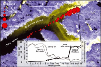
Fig. 2. MODIS satellite image of Kangerlussuaq Fjord (MODIS bands 1, 1, 2 = RGB) showing land, water and sediment-rich water exiting from the Watson River and an unnamed river, overlain by a transect of 22 in situ measurements of SSC (red circles) and other water-quality parameters collected on 3 June 2008. Inset graph shows satellite-derived MODIS reflectance, in situ field reflectance, salinity and optical depth along the transect. The estuary has three distinct water masses (see Table 1): clear water, brackish plume and plume. The plume is most responsive to inputs of glacial meltwater.
2.3. Remote sensing of suspended sediment
Plume characteristics were extracted from remotely sensed MODIS surface reflectance data. The MODIS instrument on NASA’s Terra satellite offers daily coverage over the study area, with seven bands in the visible and infrared spectra at 500 m spatial resolution and two bands at 250 m resolution. MOD09 MODIS 500 m surface reflectance product (Reference Vermote, El Saleous and JusticeVermote and others, 2002), atmospherically corrected for gases, aerosols and thin cirrus clouds, was used from 2000 to 2007 during the melt season (1 May–30 September). MODIS data are freely available and were downloaded from the NASA Warehouse Inventory Search Tool (https://wist.echo.nasa. gov/api/). A 100 km2 region of interest (ROI) larger than the maximum expected extent of the most turbid part of the plume was defined for remote-sensing analysis within the estuary.
A subset of high-quality ‘clear-sky’ MODIS images was extracted from the full MODIS dataset. High-quality clear-sky images were defined as having within the ROI: (1) a near-nadir view with adequate solar illumination (i.e. satellite overpass between 13:00 and 17:00 UTC); (2) minimal cloud cover; and (3) minimal atmospheric interference. Cloud cover was flagged using MODIS band 6 (1628–1652 nm) reflectance >0.08 to restrict the influence of thin clouds on plume reflectance. Atmospheric interference was flagged using MODIS Quality Assurance (QA) datasets that detailed various quality levels of the corrected product for each band. All images were processed in their native sinusoidal projection and a minimum of 90% quality assurance in all above descriptors.
MODIS surface reflectance was calibrated to ground-truth data by developing an empirical fit between field reflectance and field SSC. Field spectra were integrated over the spectral response of MODIS bands and compared with field SSC measurements to determine the optimal MODIS band(s) or band ratios for distinguishing the sediment-rich plume from clear water. An empirical model was developed by testing and identifying the best-fit regression model to relate various MODIS bands and band ratios to SSC.
The empirical model was applied to MODIS surface reflectance data to derive datasets of maximum plume SSC and plume area for the ROI, capturing the most turbid and optically reflective part of the plume. The maximum plume SSC was defined as the average reflectance of the 20 highest reflectance pixels of MODIS band 1 (shown in section 3; MODIS band 1 was determined to be optimal for SSC retrieval), then converted into mg L−1 to describe SSC. The plume area was defined as all pixels above a minimum MODIS band 1 (620–670 nm) reflectance value of 0.12 to characterize the extent of the most turbid areas of the plume.
2.4. Tidal influence
While other factors such as wind and sediment particle size influence sediment dispersal and surface-water circulation in estuaries, sediment plume characteristics are dominated by river discharge and tidal cycles (Reference Castaing and AllenCastaing and Allen, 1981; Reference Syvitski, Asprey, Clattenburg and HodgeSyvitski and others, 1985). Tides have been observed to influence plume behavior due to the sinking of the denser incoming ocean water spreading out the surface layer plume (Reference Dowdeswell and CromackDowdeswell and Cromack, 1991). To examine the effect of tides on remotely sensed plume area and SSC in Kangerlussuaq Fjord, the MODIS data were separated into those acquired during incoming tide and those acquired during outgoing tide at the time of satellite overpass. Time series of tidal heights were obtained for Camp Lloyd (66.97° N, 50.95° W) near the mouth of the Watson River in Kangerlussuaq Fjord (http://tbone.biol.sc.edu/tide; heights obtained through XTide version 2.8.2 software, http://www.flaterco.com). Image overpass times were compared with corresponding tidal heights to assess the importance of tidal influence on plume dynamics.
2.5. Remote sensing of supraglacial melt phenomena
Daily surface-melt extent and supraglacial lake outburst drainage are the examined supraglacial melt phenomena. Surface-melt extent was quantified using a daily ice-sheet surface-melt product previously derived from Special Sensor Microwave/Imager (SSM/I) passive microwave data (Abdalati and Steffen, 2007). The data represent melting in the surface and near-surface, but the data product is referred to hereafter as ‘surface melting’ to distinguish it from ice-sheet basal melting. Each gridcell of this product measures 25 km × 25 km and presents a binary indicator, that is melt or no melt. A daily time series of total surface-melt area was constructed by counting the number of melt pixels occurring within the 66000 km2 ice-sheet drainage basin (Fig. 1), with a maximum of 103 pixels possible, on each day. Additionally, a subset time series of rapid melt ‘expansion’ and ‘contraction’ events was also extracted from the daily surface-melt product. To qualify as a melt expansion or contraction, the melt area had to increase or decrease more than 0.75 standard deviation over the preceding day’s melt area.
Supraglacial lake drainages within the 15 000 km2 subarea of the ice sheet where lakes form (Fig. 1) were identified through image classification of MODIS surface reflectance data and confirmed by manual inspection using the methods of Reference Box and SkiBox and Ski (2007). A blue/red band ratio of band 3 (459–479 nm)/band 1 (620–670 nm) was used with a minimum threshold of 1.20 to classify lakes and measure their areas. To attain a higher spatial resolution dataset, the 500 m band 3 data were sharpened to 250 m using a band 1 ratio of (band 1 at 250 m)/(band 1 at 500 m) (L.E. Gumley and others, http://rapidfire.sci.gsfc.nasa.gov/faq/MODIS_True_Color.pdf). Lakes >0.5 km2 were classified as drained if at least 80% of their surface area was lost between clear-sky images. The same MODIS cloud-clearing criteria used for sediment plumes are applied to determine lake drainages. Due to the uncertainty from data gaps, a lake drainage ‘date’ was defined as the midpoint date between two clear-sky images, with the associated bracket in temporal uncertainty also recorded. Because multiple lake drainages can occur, lake drainage ‘events’ were defined as dates when one or more individual lake drainages was detected.
2.6. Comparison of ice-sheet surface-melt phenomena with sediment plume response
The plume datasets were analyzed with respect to the daily time series of surface melt, as well as discrete events of rapid surface-melt expansions/contractions and lake drainages, to test how sediment plumes respond to ice-sheet hydrology on long and short timescales and to distinguish between the effects of the two surface phenomena. Recall that melt expansions/contractions were defined as any increase/decrease exceeding 0.75 standard deviation over the preceding day’s melt extent. Due to data gaps in the plume time series, a further subset of melt expansions/contractions uniquely bracketed by plume data was culled from the melt events dataset. This bracketed subset was arbitrarily defined as any expansion/contraction occurring between two plume observations separated by no more than 14 days to restrict the temporal resolution of the MODIS dataset. Further, the event must be unique, that is with no other expansion/contraction occurring during this time. Based on the 30–50 km river distances between the ice margin and the estuary and an average in situ velocity measurement of 0.3 m s−1,the meltwater is expected to require over 24 hours to reach the estuary. Therefore, plume response was determined as an increase or decrease in plume area >2 days after the ice-sheet melt event. Supraglacial lake drainage events were also subset with the same restrictions, with the uncertainty of the lake drainage dates further restricting the available plume observations bracketing the event within a 14 day period.
3. Results
3.1. Plume characteristics from field campaign
The terrestrial, that is ice-sheet, origin of the Kangerlussuaq Fjord sediment plume is confirmed by the in situ water-sampling data. Low salinities, high SSC, low optical depth and high spectral reflectance are all associated with the plume feature captured in the 3 June 2008 MODIS image (Fig. 2). Furthermore, the results indicate that the estuary water masses can be divided into three types: (1) ocean-dominated clear water (hereafter called ‘clear water’) with high salinity >15 ppt, high optical depth >5 m, very low SSC <2 mg L−1 and very low spectral reflectance across all wavelengths; (2) intermediate mixing-zone waters (hereafter called ‘brackish plume’) with low salinity <7 ppt, low optical depth <2 m, low SSC <5 mg L−1 and low spectral reflectance peaking at ∼550 nm; and (3) turbid terrestrial waters (hereafter called ‘plume’) with very low salinity <3 ppt, very low optical depth <0.1 m, very high SSC >80 mg L−1 and high spectral reflectance with two peaks at ∼650 and ∼820 nm wavelength (Fig. 2; Table 1). The plume represents the most turbid and optically reflective water mass where sediment-rich meltwater first enters the estuary and rests buoyantly above the saline ocean water for some distance before mixing occurs. The brackish plume is a diffuse, spatially variable mixing zone persisting 5–65 km down-estuary from the plume. Clear water represents saline ocean water with little suspended sediment. As observed in the field and from MODIS imagery, the boundary between the plume and the brackish plume is usually sharp and distinguishable, whereas the boundary between the brackish plume and clear water is not.
Table 1. Summary of the surface-water samples collected on 3 June 2008 (see Fig. 2) for clear water, brackish plume and plume water masses. A total of 22 samples was taken along a 22 km transect and averaged into the three groups. The high-reflectance plume is used to extract temporal variations of plume area and plume SSCmax from MODIS surface reflectance imagery

3.2. MODIS retrievals of plume SSCmax and area
MODIS band 1 and a non-linear fit model relating SSC and spectral reflectance is optimal for retrievals of plume SSC (Fig. 3). The optimal spectral band for plume mapping is 620–670 nm (MODIS band 1), useful for separating plume, brackish plume and clear water as illustrated for three sample field spectra (Fig. 3a). An additional peak in plume field reflectance corresponds to MODIS band 2 (841–876 nm), but the higher percentage of pixels flagged for atmospheric correction problems in this near-infrared band ruled out the inclusion of band 2 in the final empirical model. The relationship between SSC and MODIS band 1 reflectance, developed using the field SSC and field spectra integrated over the MODIS band 1 wavelength range, is:
with R(band 1) as the reflectance (%) for MODIS band 1 and SSC measured in mg L−1. This empirical model describes the relationship between MODIS-derived reflectance and SSC very well, with the model accounting for 90% of the variability (Fig. 3b). Note that for SSC> 80 mg L−1, the MODIS band 1 reflectance saturates. This saturation likely precludes the successful quantification of very high SSC from MODIS reflectance, thus reducing the sensitivity of the maximum plume SSC measurement, hereafter called SSCmax, within the plume. However, this saturation is helpful for quantifying plume area because it allows use of a simple reflectance threshold (Fig. 3b, dashed line) to discern the plume from other water masses. Owing to its highly terrestrial origin, the plume area, A p, is used for further analysis and ‘plumes’ hereafter refer to A p unless otherwise stated.

Fig. 3. (a) Three sample field spectra representing the three water masses identified in Figure 2: plume, brackish plume and clear water. The plume was distinguished from the other two water masses by using MODIS band 1 (620–670 nm). (b) Empirical relationship between field SSC and simultaneous MODIS band 1 reflectance established from field data in Kangerlussuaq Fjord on 3 June 2008 (R 2 = 0.90). The dotted line represents the reflectance threshold (12%) used to map the plume to calculate plume area, A p.
3.3. Plume response to hydrology: interannual and seasonal
Temporal variations in the plume area A p are retrieved successfully from clear-sky MODIS images (Figs 4 and 5). A total of 235 clear-sky images is extracted from 1224 potential target days from 1 May to 30 September 2000–07 (passive microwave melt data were not available for 2008). Data gaps result from our strict high-quality definition of what constitutes a clear-sky MODIS image. The highest-quality MOD09 surface reflectance images are integral in a study relying on variations in spectral reflectance to quantify a physical water-quality process.

Fig. 4. Average seasonal development of ice-sheet surface-melt area and estuary plume area, A p, from 2000 to 2007. Melt area is averaged across the same day of the year for 8 years to produce a seasonal climatology of melt, and A p is similarly averaged over clear-sky days. A drop in A p relative to melt in late August and September suggests sediment-supply depletion towards the end of the melt season.

Fig. 5. Daily measurements of remotely sensed melt area (gray line) and plume area, A p (solid circles), from 2000 to 2007 (bottom frame), and the total area of each lake drainage event and the date of the drainage(s) (top frame) (the width of the bar indicates the range of days within which the drainage could have taken place). A total of 54 dates of lake drainage events occurred within the 8 year study.
The average seasonal evolutions of both plume area, A p, and melt area broadly co-vary (Fig. 4). The daily melt area values are averaged across the same day over 8 years to produce a seasonal climatology of melt, and the A p values were similarly averaged across clear-sky days for comparison. A relatively strong overall correlation between the seasonal averages of melt and A p (R = 0.64, p = 0.001) suggests that the estuary sediment plumes are generally synchronized with its surface-melt drivers on a seasonal scale. Figure 4 shows that, on average, plume onset quickly follows melt onset and that A p starts to decline earlier relative to melt area in September. Detailed time series of plume area, A p, and melt area for all 8 years are shown in Figure 5. In 2000, 2001, 2003, 2004 and 2007, plumes appear immediately in response to the first onset of melting on the ice sheet (Figs 5 and 6). The concurrent appearance of plumes with ice-sheet surface-melt onset only takes place when the seasonal landfast sea ice in the estuary clears up approximately at the end of May before melting begins. Otherwise, if the estuary sea ice is still present during melt onset, plume detection is delayed as seen in 2002, 2005 and 2006 (Fig. 6). Extraction of any plume information is prevented until the estuary opens up, after which the first clear-sky MODIS observation captures an already large plume area (e.g. 2005, Fig. 5). A drop in A p at the end of the season while melt extent is still high (e.g. 2003 and 2006, Fig. 5), which is very apparent in the seasonal average (Fig. 4), indicates late-season hysteresis in the relationship between melt extent and A p. Tidal influence on remotely sensed plume area in Kangerlussuaq Fjord is negligible as shown by the nearly identical plume area probability distribution functions during incoming and outgoing tides (Fig. 7).
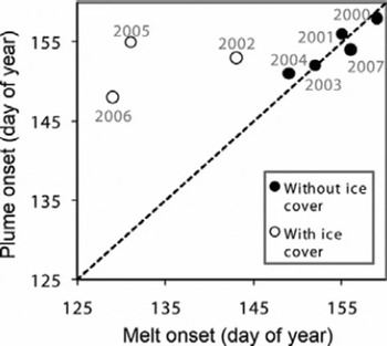
Fig. 6. Plumes appear immediately in response to ice-sheet surface-melt onset, provided the estuary is free of landfast sea ice when melting begins on the ice sheet (solid circles, grouped around a 1 : 1 line). The three years in which the estuary sea ice is still present in the estuary past melt onset exhibit later plume onset dates relative to the melt onset dates (open circles).

Fig. 7. Frequency histograms of plume area, A p, during incoming and outgoing tide, respectively, suggest little or no tidal influence upon plume area. Tidal cycles are represented by a binary indicator of incoming or outgoing tide at the MODIS image acquisition time. The frequency distributions of A p show no significant difference between incoming and outgoing tides.
Similar interannual variations in annually averaged plume and melt areas suggest that large plumes occur in high-melt years and small plumes occur in low-melt years (Fig. 8). A p is averaged annually over data gaps by interpolating between observations to allow for comparison with the average annual melt area. Figure 8 suggests that despite the seasonal hysteresis, broadly speaking the total amount of sediment-rich meltwater delivered to the ocean is proportional to the total amount of ice-sheet surface melting upon the ice sheet during that year.

Fig. 8. Interannual variations of annually averaged plume area, A p (gray circles), track those of annually averaged ice-sheet surface-melt area (black triangles) over the 2000–07 study period.
3.4. Plume response to hydrology: short-term events
Based on a small dataset, plumes appear less responsive to abrupt supraglacial hydrologic phenomena. Owing to a limited availability of high-quality clear-sky MODIS images, just 16 melt expansions and 13 melt contractions are uniquely bracketed by plume data (i.e. MODIS data are available ±1–7 days around each peak melt event) over the study area between 2000 and 2007. Of the 16 melt expansions, 11 (69%) of the melt expansions are followed by an increase in A p. Of the 13 melt contractions, 7 (54%) of the melt contractions are followed by a decrease in A p.
Similarly, supraglacial lake drainages do not clearly affect the plume area. A total of 54 lake drainage events was identified over the 8 years with 207 individual lakes (recall that lake drainage events are dates with one or more individual lake drainages) >0.5 km2 (Fig. 9; Table 2). On average, lake drainage events occurred on approximately 23 July ± 17 days with an average area of 7.7 ± 6.4 km2, and the largest individual lake drainage occurred in 2006 with a surface area of 12.3 km2 (Fig. 5; Table 2). The temporal uncertainty of the lake drainage dates, in addition to the gaps in A p, further subsets the dataset into 26 events with clear plume responses. Of these 26 lake drainage events, 10 events are followed by an increase in A p while 16 events are followed by a decrease in A p.

Fig. 9. Remotely sensed spatial distribution (MODIS bands 1, 1, 2 = RGB) of supraglacial lakes within the 15 000 km2 ice-sheet area (Fig. 1) on 8 August and 17 August in 2005. Several lakes remain intact between 8 and 17 August, except for two lakes ∼11 km2 (red circles) that drained.
Table 2. Summary of lake drainages and interannual variability of melt area and plume area, A p. Lake drainage events are dates with one or more individual lake drainages >0.5 km2 and summarized as a total surface area for each date. Interannual variability of both melt area and A p is determined by averaging over each year

4. Discussion and Conclusion
Hydrologic observations are needed to assess the discharge of water from the Greenland ice sheet, but field-based measurements are difficult to procure or simply unavailable. This first remote-sensing study of Greenland sediment plume dynamics suggests they offer a unique metric of ice-sheet meltwater discharge.
The response of estuary plumes to ice-sheet meltwater production is clearest on the seasonal or interannual scales (Fig. 8). Plumes appear quickly upon initial onset of surface melting (Fig. 6), indicating a rapid coupling between the ice sheet and the estuary each spring. This observation lends support to the idea of a rapid linkage between surface and basal hydrology (Reference Zwally, Abdalati, Herring, Larson, Saba and SteffenZwally and others, 2002; Reference Bartholomaus, Anderson and AndersonBartholomaus and others, 2008; Reference Van de WalVan de Wal and others, 2008; Reference Shepherd, Hubbard, Nienow, McMillan and JoughinShepherd and others, 2009) and suggests meltwater rapidly escapes to the ocean. Furthermore, the surface and proglacial ‘exit’ hydrology are coupled at the interannual scale, meaning there is no evidence that large volumes of water generated on the ice-sheet surface are stored within the ice sheet only to escape in some following year. In general, the meltwater exported to the ocean appears to be proportional to the meltwater produced, with highest-melt years associated with the highest export of meltwater.
While abrupt melt fluctuations on the ice sheet appear less perceptible, 11 out of 16 melt pulses on the ice sheet did trigger an increase in plume area, A p. Melt contractions did not clearly trigger a decrease in A p, but they should not have been expected to because contractions in Ap are mainly due to mixing of the plume with marine water rather than short-term reductions in meltwater input. Put another way, plume development might be expected to expand more readily in response to new infusions of meltwater rather than to contract in response to declines in meltwater. Other short-term phenomena (e.g. rainfall, early season terrestrial snowmelt and outburst floods from proglacial lakes along the ice margin) were not explored and may also influence plume dynamics.
Our data suggest that few if any lake drainages result in sudden releases of meltwater to the ocean: only 10 of 26 drainage events (38%) produced perceptible increases in plume area. Although this finding suggests that plumes are not sensitive to short-term lake drainage events, it is plausible that a more comprehensive dataset, or another technique better suited for detecting short-term phenomena, may show stronger links between lake drainages and meltwater export. For example, a lake drainage event (0.044 km3) observed by Reference DasDas and others (2008) had a volume fourfold greater than that of a recorded burst of meltwater (0.011 km3) into the Watson River, and in principle was more than large enough to influence plume area. Another possibility is that water from lake drainages is either diffused within well-distributed subglacial drainage networks, which is hypothesized to produce a spatially uniform increase in ice-sheet velocities (Reference DasDas and others, 2008; Reference JoughinJoughin and others, 2008a), or is stored englacially or at the bed, thus failing to exit the ice sheet within the timescales investigated here. How meltwater moves through the ice sheet is an important unresolved question addressing the mechanism of melt-induced acceleration, as lake drainages have been linked to the speed-up of Russell Glacier within our study region (Reference McMillan, Nienow, Shepherd, Benham and SoleMcMillan and others, 2007).
The estuary plumes and ice-sheet melt co-vary broadly from the early to mid-season, but the earlier drop in A p relative to melt area occurs by September of each year (Fig. 4). Two possible explanations for this hysteresis are: (1) water retention within the ice sheet; or (2) late-season sediment-supply exhaustion. In the first case, ice-sheet runoff may decline despite continued surface melting, indicating that water produced by surface melt becomes retained or densified (Reference Pfeffer, Meier and IllangasekarePfeffer and others, 1991; Reference ReehReeh, 2008). This may occur at the end of the melt season, with greater freezing at night (Reference Nghiem, Steffen, Kwok and TsaiNghiem and others, 2001; Reference Ramage and IsacksRamage and Isacks, 2003), which may not be perceptible in the daily melt extent dataset. Additionally, the passive microwave melt time series is a measure of melt area and not intensity, which may be more directly related to sediment flux. The second case presents another possibility, namely that the observed hysteresis indicates a late-season exhaustion of transportable sediments. Sediment-supply hysteresis is found in proglacial streams across a range of temporal scales (Reference Willis, Richards and SharpWillis and others, 1996), including seasonal (Reference Schneider and BrongeSchneider and Bronge, 1996). Loose sediments available following freezing and thawing during the winter would flush immediately during melt onset and while the subglacial drainage network is reopened each year, leaving the more resistant materials and decreasing the availability of transportable sediment as the melt season progresses (Reference Hammer and SmithHammer and Smith, 1983). Long-term discharge data and SSC measurements are needed to further evaluate these hypotheses.
Our study shows that plumes are best identified as the surface area of the plume, A p. The highly turbid plume, with sharp fronts clearly visible dividing it from the dispersed plume, derives nearly wholly from terrestrial meltwater sources and is most immediately responsive to changes in freshwater discharge. It is also highly reflective in MODIS band 1 (620–670 nm), and while red and near-infrared bands (Reference Hu, Chen, Clayton, Swarzenski, Brock and Muller-KargerHu and others, 2004) and band ratios (Reference Doxaran, Froidefond and CastaingDoxaran and others, 2003) are conventionally used to identify mineral sediment, we find that MODIS band 1 is sufficient to determine sediment in agreement with Reference Miller and McKeeMiller and McKee (2004). Though quantification of SSC is successful for waters with very low sediment concentrations (<60 mg L−1) (Reference Hu, Chen, Clayton, Swarzenski, Brock and Muller-KargerHu and others, 2004; Reference Miller and McKeeMiller and McKee, 2004) where the relationship with reflectance is linear, it does not work as well in an estuary with high sediment concentrations like Kangerlussuaq Fjord where the relationship is non-linear and shows saturation. Fortuitously, the reflectance saturation that occurs with high sediment concentrations provides a threshold for quantifying A p (Fig. 3b), allowing the plume area to be measured easily.
While this study explored land-terminating outlet glaciers, the technique could also be applied to marine-terminating glaciers. However, in the case of marine-terminating glaciers, the presence of calving ice in the water will confound the remotely sensed signal. Reference Lewis and SmithLewis and Smith (2009) estimate 350 outlets where runoff from the Greenland ice sheet reaches the ocean, either through rivers or directly from tidewater glaciers. Although 324 of those are land-terminating glaciers and only 26 are marine-terminating glaciers (that are confirmed by observations of sediment output as meltwater outlets), studies of marine-terminating outlet glaciers are of utmost value because they contribute the majority of the ice mass discharge (Reference Rignot and KanagaratnamRignot and Kanagaratnam, 2006; Reference Howat, Smith, Joughin and ScambosHowat and others, 2008a; Reference Joughin, Das, King, Smith, Howat and MoonJoughin and others, 2008b). Future work should examine the spatial and temporal characteristics of meltwater release for all potential hydrologic exits from the Greenland ice sheet, including marine-terminating outlet glaciers.
Sediment plumes from Greenland outlet glaciers are an indicator of ice-sheet meltwater export to the estuary, with the plume area increasing (decreasing) in response to increasing (decreasing) surface-melt area. The strength of the relationship is most robust at the interannual scale, while shorter-term ice-sheet events are more difficult to distinguish in the plumes. The limited measurements of discharge have hindered efforts to understand the temporal and spatial variations of ice-sheet meltwater release into the ocean, but now remote sensing provides a technique for describing the hydrologic output from remote areas by observing sediment plumes as an indicator of water flow. The ramification of this study is that now the relationship between ice-sheet melt and meltwater reaching the ocean can be characterized for outlet glaciers around Greenland, providing insights into future contributions to sea-level rise.
Acknowledgements
This work was supported by the NASA Cryospheric Sciences Program grant NNG05GN89G and grant NNGO6GB70G, and the MODIS imagery was also provided by NASA. We thank Kangerlussuaq International Science Support for providing logistical support for fieldwork. We also thank R. Carlos for laboratory processing of field samples, P. Levine for data-processing code, and L. Apper, E. Lyons and two reviewers for their careful reading of the manuscript.


