


1. Introduction
Mass transfer between a dispersed gas and a liquid phase is a general phenomenon encountered in industrial processes (bubbly columns, chemical or bio-reactors) as well as environmental flows (breaking waves, lake aeration systems,  $\ldots$). Both the bubble deformation and the surface contamination influences the rate of gas dissolution (Levich Reference Levich1962; Clift, Grace & Weber Reference Clift, Grace and Weber1978; Takemura & Yabe Reference Takemura and Yabe1999), it is therefore crucial to address their coupled effects on the bubble dynamics and mass transfer performance.
The bubble shape, during its rise motion, results from the competition between deforming stresses due to the outer flow, which are of inertial nature at high Reynolds number  $Re$ (based on the bubble rise velocity), and the capillary stresses which resist to deformation. For ellipsoidal bubbles, the distortion can be well characterised by the aspect ratio $\chi$. In the case of clean bubbles, several theories or correlations have been proposed to quantify $\chi$: the potential flow theory with a rotational correction to include dissipation from the boundary layer by Moore (Reference Moore1965); or predictions issued from experimental or numerical investigations by Clift et al. (Reference Clift, Grace and Weber1978), Ryskin & Leal (Reference Ryskin and Leal1984a,Reference Ryskin and Lealb), Duineveld (Reference Duineveld1995), Loth (Reference Loth2008), Rastello, Marié & Lance (Reference Rastello, Marié and Lance2011), Legendre, Zenit & Rodrigo Velez-Cordero (Reference Legendre, Zenit and Rodrigo Velez-Cordero2012) and Sharaf et al. (Reference Sharaf, Premlata, Tripathi, Karri and Sahu2017). In these works, $\chi$ is a function of two dimensionless parameters among the Weber, Morton, Reynolds or Eötvös numbers. Besides, the drag coefficient $C_{D}$ of clean bubbles at large Reynolds number has also been widely studied (Moore Reference Moore1963, Reference Moore1965; Duineveld Reference Duineveld1995; Veldhuis Reference Veldhuis2007; Dijkhuizen et al. Reference Dijkhuizen, Roghair, Van Sint Annaland and Kuipers2010; Rastello et al. Reference Rastello, Marié and Lance2011) in the case of either spherical or oblate bubble shapes.
Regarding the gas–liquid mass transfer around ellipsoidal bubbles, it has been theoretically investigated by Lochiel & Calderbank (Reference Lochiel and Calderbank1964) in the case of either fully mobile or immobile interfaces, at high Schmidt ( $Sc$) and Péclet numbers. In the case of very large Reynolds number, for interfaces with a slip condition, the authors provided an analytical expression of the Sherwood number $Sh$ based on the potential flow theory: they introduced a correction based on $\chi$ to the Sherwood number of a spherical bubble from Boussinesq (Reference Boussinesq1905), which revealed that the effect of bubble eccentricity is very small provided that the bubble is an oblate spheroid. Later, Figueroa-Espinoza & Legendre (Reference Figueroa-Espinoza and Legendre2010) investigated the external mass transfer around a clean ellipsoidal bubble based on boundary-fitted numerical simulations. The authors confirmed this unexpected finding: the $Sh$ for clean deformed bubbles can be reasonably well evaluated by the Boussinesq solution for spheres in a large range of Schmidt and Reynolds numbers, provided that the equivalent diameter is used as the characteristic length to define the Péclet number. They proposed corrective functions $f(\chi )$ in order to adjust the solution for ellipsoidal bubbles with $\chi \leq 3$ at several $Re$, by noting that the correction is less than 10 $\%$ for $Re \geq 100$.
For the applications, configurations of interest are, however, generally rich in contaminants and surfactants, i.e. amphiphilic molecules which adsorb to the interfaces and affect the surface tension. At large concentration, surfactants can confer complex rheological properties to the interfacial film, which are elastic and viscous properties, either due to the variation of the chemical composition of the interface or to interactions between the adsorbed surfactants, as classified by Verwijlen, Imperiali & Vermant (Reference Verwijlen, Imperiali and Vermant2014). As bubble surfaces are particularly sensitive to their surroundings (Dollet, Marmottant & Garbin Reference Dollet, Marmottant and Garbin2019), this induces huge consequences on the bubbly flows. In this way, even when only traces of surfactants are present, in such a way that the surface tension remains very close to that of a clean interface, contaminants provide a Gibbs elasticity to the bubble surface, and significantly affects the interfacial motion (Lakshmanan & Ehrhard Reference Lakshmanan and Ehrhard2010; Lalanne, Masbernat & Risso Reference Lalanne, Masbernat and Risso2020; Manikantan & Squires Reference Manikantan and Squires2020) through Marangoni stresses. As a consequence, a small concentration of adsorbed surfactants is sufficient to drastically impact the hydrodynamics and rates of transfer across the interface, including significant effects on the drag force (Levich Reference Levich1962; Cuenot, Magnaudet & Spennato Reference Cuenot, Magnaudet and Spennato1997; Zhang & Finch Reference Zhang and Finch2001; Pesci et al. Reference Pesci, Weiner, Marschall and Bothe2018), the lift force (Takagi & Matsumoto Reference Takagi and Matsumoto2011; Hessenkemper et al. Reference Hessenkemper, Ziegenhein, Lucas and Tomiyama2021; Atasi et al. Reference Atasi, Ravisankar, Legendre and Zenit2023) or the bubble path instabilities that surfactants can trigger (Tagawa, Takagi & Matsumoto Reference Tagawa, Takagi and Matsumoto2014) since they depend on the vorticity production at the interface.
Surfactants are known to decrease the bubble rise velocity down to the one of a solid sphere of the same size in the worst case (Zhang & Finch Reference Zhang and Finch2001): the velocity of the fluid at the interface is retarded due to the Marangoni stresses, caused by the surface tension gradients resulting from the advection of the surfactants along the surface (Levich Reference Levich1962; Clift et al. Reference Clift, Grace and Weber1978; Bel Fdhila & Duineveld Reference Bel Fdhila and Duineveld1996; Takemura Reference Takemura2005; Takagi & Matsumoto Reference Takagi and Matsumoto2011). In practical conditions, surfactants are soluble: they adsorb continuously from the bulk phase to the interface, mostly at the front of the bubble, then are convected towards the rear of the bubble where the locally high concentration leads to desorption (Cuenot et al. Reference Cuenot, Magnaudet and Spennato1997; Palaparthi, Demetrios & Maldarelli Reference Palaparthi, Demetrios and Maldarelli2006). The present study focuses on the configuration where the rate of surface convection of surfactants is much higher than (i) the rate of exchange between the bulk and the interface (limited by either transport in the bulk or adsorption kinetics) and (ii) the rate of surface diffusion. In that case, surfactants can be assumed to be insoluble: the adsorption/desorption rates are neglected. This regime results in a characteristic stagnant-cap angle  $\theta _{cap}$ formed by the advected surfactants at the rear of the bubble, which splits the surface into a part with mobile interface and another one with immobile interface, as illustrated in figure 1. In the case of contaminated spherical bubbles, the reduced drag coefficient is known to be a function of $\theta _{cap}$ from the works of Sadhal & Johnson (Reference Sadhal and Johnson1983), Zhang & Finch (Reference Zhang and Finch2001) and Piedfert et al. (Reference Piedfert, Lalanne, Masbernat and Risso2018). Concerning the case of oblate bubbles, Dijkhuizen et al. (Reference Dijkhuizen, Roghair, Van Sint Annaland and Kuipers2010) reported that experimental drag coefficients are mostly higher than in pure systems, due to the presence of impurities. From comparisons between numerical simulations and experiments, they suggested that contamination induces much less deformed bubbles. Empirical models have been proposed for the drag coefficient of deformed bubbles in the presence of surfactants, depending on $(Re,Eo)$ by Tomiyama et al. (Reference Tomiyama, Kataoka, Zun and Sakaguchi1998) or on $(Re,\chi )$ by Chen et al. (Reference Chen, Hayashi, Hosokawa and Tomiyama2019) for a fully contaminated interface, but there is no general correlation relating the drag coefficient to the stagnant-cap angle of contamination for intermediate cases. Regarding the aspect ratio, Aoyama et al. (Reference Aoyama, Hayashi, Hosokawa and Tomiyama2018) analysed the bubbles’ shapes in liquid solutions where Triton X-100 and 1-octanol were added as surfactants: the interfaces were considered as fully immobile since the point where the drag coefficient is independent on the surfactant concentration was reached. They proposed an empirical correlation $\chi (Re,Eo)$ to predict the aspect ratio, validated in the basis of experimental data involving other types of surfactants: sodium dodecyl sulphate (SDS), 1-decanol. Generality of their correlation in the case of contaminated bubbles is still an open question. A systematic investigation on the influence of surfactants on the bubble deformation is therefore not yet achieved.

Figure 1. Deformed rising bubble in a quiescent liquid: representation of the contamination angle  $\theta _{cap}$ in the stagnant-cap regime.
Regarding gas–liquid mass transfer in the presence of surfactants, it has been reported by several experimental or numerical investigations that the rate of transfer declines for an interface which includes a (partial) no-slip condition (Garner & Hale Reference Garner and Hale1953; Takemura & Yabe Reference Takemura and Yabe1999; Vasconcelos, Orvalho & Alves Reference Vasconcelos, Orvalho and Alves2002; Jimenez et al. Reference Jimenez, Dietrich, Grace and Hebrard2014; Weiner et al. Reference Weiner, Timmermann, Pesci, Grewe, Hoffmann, Schlüter and Bothe2019; Dani et al. Reference Dani, Cockx, Legendre and Guiraud2021; Lebrun et al. Reference Lebrun, Xu, Le Men, Hébrard and Dietrich2021; Abadie et al. Reference Abadie2022): when increasing the contamination rate, the Sherwood number of a spherical bubble decreases from the prediction for a clean bubble, given by Colombet et al. (Reference Colombet, Legendre, Cockx and Guiraud2013) and Takemura & Yabe (Reference Takemura and Yabe1998), until the value for a solid sphere, estimated by Ranz & Marshall (Reference Ranz and Marshall1952) and Frössling (Reference Frössling1938). In particular, provided that the bubbles are spherical, and in a case where the adsorption and desorption rates of surfactants are very slow (leading to the stagnant-cap regime), the decline of the Sherwood number was previously investigated, by means of direct numerical simulations by Kentheswaran et al. (Reference Kentheswaran, Dietrich, Tanguy and Lalanne2022). This work revealed that the mass transfer decrease results from both (i) the decrease of the bubble rise velocity due to the partial interface immobilisation, and (ii) local phenomena related to the progressive change of hydrodynamics, even in the remaining mobile part of the interface. Indeed, on the one hand, in the mobile part, the tangential velocity of the fluid is lower than for a clean bubble at the same  $Re$, which reduces mass transport: this was characterised by a dimensionless maximum tangential velocity $u_{max}^{*}$, normalised by that around a bubble with slip condition. On the other hand, the part of the interface which is immobilised induces a thicker mass boundary layer for the transfer of the solute, i.e. a lower contribution of $Sc$ in the global Sherwood number. Finally, a correlation to predict $Sh$ around contaminated bubbles has been proposed, based on both global ( $Re$,
$Re$,  $Sc$) and local parameters ( $\theta _{cap}$, $u_{max}^{*}$). However, such a correlation has been established only in the case of spherical gas bubbles, without taking into account the impact of distortion on the transfer rate.
Here, direct numerical simulations of rising deformable bubbles in the stagnant-cap regime are performed, in order to mimic the effect of a monolayer of surfactants present in dilute concentration at the interface (no interaction between surfactant molecules at the interface is modelled). Surfactants are considered as insoluble: they are already adsorbed on the interface and are only transported along the bubble surface. The numerical approach consists in solving the Navier–Stokes equations with the Marangoni stresses as a jump condition on the tangential stresses at the interface. A parametric study is carried out, by defining seven cases at given Archimedes and Eötvös numbers, and by increasing the amount of surfactant so as to vary the Marangoni number. In this way, each case represents the progressive contamination of rising bubbles of given properties, in the inertial regime where oblate shapes are obtained. The contamination angle  $\theta _{cap}$, the bubble aspect ratio $\chi$ and the Reynolds number are not imposed but result from the numerical computation.
Axisymmetric conditions are assumed: as the range of investigated Reynolds numbers is between 10 and 70, the flow is always stable, below the limit of path instability known for an ellipsoidal clean bubble, given by Magnaudet & Mougin (Reference Magnaudet and Mougin2007), or reported for oblate bubbles in the presence of surfactants by Tagawa et al. (Reference Tagawa, Takagi and Matsumoto2014).
Besides, the mass transfer of a passive scalar dissolving from the gas to the liquid phase is also computed around the contaminated distorted bubble, at several Schmidt numbers. It is assumed that the solute is dilute enough (low mass flux) so that the bubble volume remains constant. The rate of mass transfer is then computed at steady state, in the form of a Sherwood number.
The main objectives of this paper are to investigate the impact of surfactants on the drag coefficient and the bubble distortion, then to analyse the consequences on the Sherwood number describing the gas–liquid mass transfer rate, in the case of bubbles with a portion of the interface which is immobile.
2. Governing equations and numerical methods
2.1. Mathematical formalism, simulation conditions
In this study, an incompressible flow is considered, described by the following mass and momentum conservation laws, in a one-fluid approach:
 \begin{gather} \rho \left( \frac{{\rm D}\boldsymbol{u}}{{\rm D}t} + (\boldsymbol{u} \boldsymbol{\cdot} \boldsymbol{\nabla}) \boldsymbol{u} \right) ={-} \boldsymbol{\nabla} p + \boldsymbol{\nabla} \boldsymbol{\cdot} (2 \mu \boldsymbol{\mathsf{D}}) + \rho \boldsymbol{g} + \sigma \kappa \delta_{I} \boldsymbol{n} , \end{gather}
 \begin{gather} \boldsymbol{\nabla} \boldsymbol{\cdot} \boldsymbol{u} = 0 , \end{gather}
where  $\rho$ and $\mu$ are, respectively, the fluid density and viscosity, $\boldsymbol {u}$ the velocity field, $p$ the pressure, $\boldsymbol{\mathsf{D}}$ the rate of deformation tensor, $\boldsymbol {g}$ the gravity acceleration, $\sigma$ the surface tension, $\kappa = - \boldsymbol {\nabla } \boldsymbol {\cdot } \boldsymbol {n}$ the interface curvature, $\delta _{I}$ the Dirac distribution centred on the interface, and $\boldsymbol {n}$ the interface normal vector. The jump condition on the normal stresses due to the capillary force is considered according to the following equation:
 \begin{equation} [\boldsymbol{n} \boldsymbol{\cdot} \boldsymbol{\tau} \boldsymbol{\cdot} \boldsymbol{n}] = \sigma \kappa , \end{equation}
where  $\boldsymbol {\tau } = -p \boldsymbol{\mathsf{I}} + 2\mu \boldsymbol{\mathsf{D}}$ is the stress tensor, and $[\boldsymbol {\cdot }]$ stands for the interface jump condition operator between liquid and gas. As both the tangential and the normal velocity (no phase change due to mass transfer is considered) are continuous across the interface, the following equation is satisfied:
 \begin{equation} [\boldsymbol{u}] = \boldsymbol{0}. \end{equation}
The transport of surfactants along the deforming bubble surface is considered, through the surface advection–diffusion equation (Levich Reference Levich1962; Stone Reference Stone1990),
 \begin{equation} \frac{\partial \varGamma}{\partial t} + \boldsymbol{u_{s}} \boldsymbol{\cdot} \boldsymbol{\nabla}_{s} \varGamma + \varGamma \boldsymbol{\nabla}_{s} \boldsymbol{\cdot} \boldsymbol{u} = D_{s} \Delta_{s} \varGamma, \end{equation}
where  $\varGamma$ is the surface concentration of surfactants, $\boldsymbol {u_{s}}$ the tangential velocity of the fluid at the interface, $\boldsymbol {\nabla }_{s} = ( \boldsymbol{\mathsf{I}} - \boldsymbol {n} \otimes \boldsymbol {n} ) \boldsymbol {\nabla }$ the surface gradient operator, $D_{s}$ the surface diffusion coefficient and $\Delta _{s}$ the surface Laplacian operator. Note that the partial time derivative of (2.5) is written along the normal direction to the interface. Equation (2.5) is solved by using an extended $\tilde {\varGamma }$ field in the normal direction to the interface, as defined in the following section. Note that an infinite surface Péclet number for the surfactant transport is assumed, based on typical values of the surface diffusion coefficient as given by Valkovska & Danov (Reference Valkovska and Danov2000), allowing us to neglect the surface diffusion term. The Marangoni interfacial stresses are taken into account as a jump condition of the tangential viscous stresses across the interface,
 \begin{equation} [\boldsymbol{t} \boldsymbol{\cdot} \boldsymbol{\tau} \boldsymbol{\cdot} \boldsymbol{n}] ={-}\boldsymbol{t} \boldsymbol{\cdot} \boldsymbol{\nabla}_{s} \sigma, \end{equation}
with  $\boldsymbol {t}$ the tangential vector to the interface.
The surface tension  $\sigma$ depends on the local surfactant concentration. Here, it is assumed to follow a Henry isotherm,
 \begin{equation} \sigma = \sigma_{0} - R_{g} T \varGamma, \end{equation}
where  $\sigma _{0}$ is the surface tension of reference around which its variations are linearised, $R_{g}$ the gas constant and $T$ the temperature. Note that (2.7) corresponds to a perfect gas model, which does not take into account any interaction between the adsorbed molecules. All the computations are performed by using this model for the surface tension.
Regarding the mass transfer of a single species from the gas to the bulk liquid, the concentration field  $C$ in the liquid phase is computed by means of the convection–diffusion equation (resistance to mass transfer is considered to be only in the external liquid phase),
 \begin{equation} \frac{\partial C}{\partial t} + \boldsymbol{u} \boldsymbol{\cdot} \boldsymbol{\nabla} C = D \boldsymbol{\nabla} \boldsymbol{\cdot} (\boldsymbol{\nabla} C) , \end{equation}
where  $D$ is the diffusion coefficient associated with the dilute binary mixture.
Here, axisymmetric simulations are performed. The system of (2.1), (2.2), (2.5) is computed until steady-state in the frame moving with the bubble, with their jump and boundary conditions, to compute the hydrodynamics of the deformed bubbles in the presence of surfactants. Then (2.8) is solved on the converged hydrodynamics.
2.2. Numerical methods
The equations presented in the previous section are implemented in the in-house code DIVA (Tanguy, Menard & Berlemont Reference Tanguy, Menard and Berlemont2007; Lalanne et al. Reference Lalanne, Rueda Villegas, Tanguy and Risso2015b; Lepilliez et al. Reference Lepilliez, Popescu, Gibou and Tanguy2016; Rueda Villegas et al. Reference Rueda Villegas, Tanguy, Castanet, Caballina and Lemoine2017). The latter has been validated on problems involving the shape oscillation dynamics of rising bubbles in Lalanne et al. (Reference Lalanne, Abi Chebel, Vejražka, Tanguy, Masbernat and Risso2015a), mass transfer around bubbles in Butler et al. (Reference Butler, Cid, Billet and Lalanne2021) and the effect of surfactants by Piedfert et al. (Reference Piedfert, Lalanne, Masbernat and Risso2018) and Kentheswaran et al. (Reference Kentheswaran, Dietrich, Tanguy and Lalanne2022).
The interface is captured by a level set distance function  $\phi$, and its evolution is obtained by solving the following convection equation:
 \begin{equation} \frac{\partial \phi}{\partial t} + \boldsymbol{u} \boldsymbol{\cdot} \boldsymbol{\nabla} \phi = 0 , \end{equation}
where negative and positive values of  $\phi$, respectively, correspond to the gas and liquid phases. In order to maintain $\phi$ as a signed distance function, a reinitialisation step is used at each time step, as proposed in Sussman, Smereka & Osher (Reference Sussman, Smereka and Osher1994).
An extrapolation  $\tilde {\varGamma }$ of the surfactant concentration $\varGamma$ is defined on both side of the interface at each time step, so as to be constant in the normal direction, by solving the following equation during a fictitious time $\tau$:
 \begin{equation} \frac{\partial \tilde{\varGamma}}{\partial \tau} + {\rm sign}(\phi)\boldsymbol{n} \boldsymbol{\cdot} \boldsymbol{\nabla} \tilde{\varGamma} = 0 . \end{equation}
Then, in the numerical implementation, (2.5) is solved on the field  $\tilde {\varGamma }$, which enables us to compute the time derivative as the usual Eulerian derivative, as developed in Pereira & Kalliadasis (Reference Pereira and Kalliadasis2008), and which facilitates the calculation of the surface convection term from the gradient of $\tilde {\varGamma }$ as its derivative in the normal direction is zero (see validation of this implementation in Piedfert et al. (Reference Piedfert, Lalanne, Masbernat and Risso2018)).
The incompressible Navier–Stokes equations are solved by a projection method. In order to ensure a sharp description of the jump conditions across the interface, both in the normal and tangential direction, the discontinuities are taken into account by the ghost fluid method (Fedkiw et al. Reference Fedkiw, Aslam, Merriman and Osher1999). In the normal direction (2.3), the pressure and viscous normal stress discontinuities are computed following the ghost fluid conservative viscous method presented in Lalanne et al. (Reference Lalanne, Rueda Villegas, Tanguy and Risso2015b), or Lepilliez et al. (Reference Lepilliez, Popescu, Gibou and Tanguy2016) with implicit formulation. In the tangential direction (2.6), the jump condition due to the Marangoni stress is computed by means of the ghost fluid primitive viscous method, originally proposed by Kang, Fedkiw & Liu (Reference Kang, Fedkiw and Liu2000), and further described in Lalanne et al. (Reference Lalanne, Rueda Villegas, Tanguy and Risso2015b). In this way, the tangential force at the interface, calculated from the gradients of surface tension, is included in the viscous stress tensor jump, on the basis of the expression provided by Piedfert et al. (Reference Piedfert, Lalanne, Masbernat and Risso2018) or Kentheswaran et al. (Reference Kentheswaran, Dietrich, Tanguy and Lalanne2022). A detailed validation of this methodology is shown in Dalmon et al. (Reference Dalmon, Kentheswaran, Mialhe, Lalanne and Tanguy2020).
In the equations, all the convection terms are computed with a fifth-order weighted essentially non-oscillatory (WENO-Z) scheme while the diffusion terms are discretised by using second-order schemes, and temporal derivatives are treated with a second-order Runge–Kutta scheme. A blackbox multigrid (BBMG) solver from Dendy (Reference Dendy1982) permits us to efficiently compute the Poisson equation resulting from the projection step.
Finally, concerning the resolution of (2.8) for the solute mass transfer from the gas to the liquid, the concentration  $C_{int}$ is assumed to be known at the interface and to remain constant, following the standard Henry law. In this paper, any potential hindrance effect associated with the presence of surfactants at the bubble surface, as discussed by Bothe (Reference Bothe2022), is neglected. In the simulation, $C_{int}$ is set by an immersed Dirichlet boundary condition at the interface (Gibou et al. Reference Gibou, Fedkiw, Cheng and Kang2002). In order to propose an accurate calculation of the concentration gradients and their transport around the interface, quadratic extrapolations of the concentration field in the liquid phase are computed inside the bubble, following the methodology from Aslam (Reference Aslam2003).
2.3. Numerical procedure and boundary conditions
In the simulations, the bubble is initialised as spherical, but only the final state is analysed, once the bubble is steadily deformed. The rising bubble is maintained at the centre of the domain of size  $l_{r} \times l_{z} = 8 R_{eq} \times 16 R_{eq}$ (it has been verified that the domain size is sufficient to neglect the confinement in the channel for the bubble Reynolds number values of the present simulations), by means of a method similar to Mougin & Magnaudet (Reference Mougin and Magnaudet2002).
For the velocity field, symmetric and wall conditions are, respectively, imposed at  $r = 0$ and $r = l_{r}$, and free boundary conditions are imposed at the top and bottom boundaries.
First, the hydrodynamics of the rising bubble in the presence of the adsorbed surfactants is computed at steady-state. Then, mass transfer is solved based on the converged velocity field. The following boundary conditions are imposed for the concentration field of the solute: a Dirichlet condition  $C_{int} = 1$ at the bubble surface, a Neumann condition with a zero flux at $r = 0$ and Dirichlet conditions with $C_{\infty } = 0$ at $r = l_{r}$, $z = 0$ and $z = l_{z}$.
3. Statement of the problem
The simulations are performed at constant density and viscosity ratios of  $815$ and $63$, respectively, which corresponds to an air bubble in water. Three other dimensionless parameters are required to characterise the hydrodynamics of contaminated and deformable bubbles: the Archimedes number $Ar$,
$Ar$,
 \begin{equation} Ar = \frac{g {d_{eq}}^{3} \rho_{liq} (\rho_{liq} - \rho_{gas})}{{\mu_{liq}}^{2}} ; \end{equation}
the Eötvos (or Bond) number  $Eo$ as the ratio between gravitational to capillary forces,
 \begin{equation} Eo = \frac{(\rho_{liq} - \rho_{gas}) g d_{eq}^2}{\bar{\sigma}} ; \end{equation}
and the Marangoni number  $Ma$ as the ratio between the Marangoni over the viscous stresses,
 \begin{equation} Ma = \frac{R_{G} T \bar{\varGamma}}{\mu_{liq} U_{\infty} } . \end{equation}
These are chosen to define the cases, where  $\bar {\sigma }$ is the average surface tension, $\bar {\varGamma }$ the average surfactant concentration obtained once the bubble shape is converged, $U_{\infty }$ the rising velocity at steady state, and $d_{eq}$ the equivalent diameter (i.e. the diameter that a spherical bubble of same volume would have). Other parameters are relevant to analyse the results, such as the Reynolds number $Re$,
$Re$,
 \begin{equation} Re = \frac{\rho_{liq} U_{\infty} d_{eq}}{\mu_{liq}} , \end{equation}
the Weber number  $We$ as the ratio between inertial and capillary stresses,
 \begin{equation} We = \frac{\rho_{liq} U_{\infty}^{2} d_{eq}}{\bar{\sigma}} \end{equation}
and the bubble aspect ratio  $\chi$ as the ratio between the large axis and the small one.
The set of parameters are chosen to obtain ellipsoidal bubble shapes from the diagram of Clift et al. (Reference Clift, Grace and Weber1978). First, simulations of different bubbles with fully mobile interfaces ( $Ma = 0$) have been performed at different couples $(Ar,Eo)$, to define seven cases, listed in table 1, with $Re^{clean}$ and $\chi ^{clean}$ as reference values for each one.
Table 1. Simulation conditions for the clean bubble cases. Each one serves as a basis for the simulations in the presence of different concentration of adsorbed surfactants, for which the parameters are shown in the Appendix.

Then, for each case at given  $Ar$, simulations are carried out in the presence of insoluble surfactants by considering a surface concentration of the latter at the interface, leading to a value of the Marangoni number $Ma$ and an Eötvös number $Eo$ which is nearly conserved compared with $Eo^{clean}$. Indeed, note that, based on the chosen values (see the Appendix), $Eo$ varies less than 5 $\%$ when varying the surfactant concentration (due to the variation of the average surface tension), except for Case 4 for which $Eo$ differs from $Eo^{clean}$ by 16 % at most.
Let us also remark that, as the bubble is initialised spherical, of diameter  $d_{eq}$, and covered by a given concentration of insoluble surfactants, both its surface area $S(t)$ and its average concentration $\bar {\varGamma }(t)$ evolve during the simulation, as the total mass of adsorbed surfactant $\bar {\varGamma }(t) S(t)$ is conserved.
In this study,  $500 \leq Ar \leq 5600$, $0.7 \leq Eo \leq 11.4$ and $0 \leq Ma \leq 20$, leading to rising bubbles in inertial conditions at moderate Reynolds numbers $10 \leq Re \leq 70$, with aspect ratios $1 \leq \chi \leq 3$. The contamination angle $\theta _{cap}$ is a direct result from the numerical resolution, cases between $\theta _{cap} = 0$ and $\theta _{cap} = {\rm \pi}$ are obtained for each simulation case.
In order to quantify the variations of surface tension along an interface when it is submitted to a deformation, the Gibbs elasticity is defined as
 \begin{equation} -\bar{\varGamma} \dfrac{{\rm d} \sigma}{{\rm d} \varGamma} = R_G T \bar{\varGamma} , \end{equation}
in the case of insoluble surfactants and based on the isotherm used for this study (2.7). The Gibbs elasticity is then normalised by the average surface tension, leading to the dimensionless elasticity number  $E$,
$E$,
 \begin{equation} E = \frac{R_{g} T \bar{\varGamma}}{\sigma_0} . \end{equation}
Here, from the values of  $\bar {\varGamma }$ at steady state, the elasticity number varies from $E = 0.02$ to $E = 0.66$, giving a wide range of applicability: from weak surface-active effects (very small $E$), which correspond to the case of residual contaminants at an interface like impurities, to stronger impacts on surface tension due to a higher surfactant concentration.
Regarding the gas–liquid mass transfer computation, the concentration field of the solute is solved at different Schmidt numbers  $Sc$ by varying the molecular diffusivity, from $Sc = 1$ to $Sc = 100$. Simulations then allow us to compute the global mass transfer rate around the deformed bubble.
4. Results on the hydrodynamics
In this section, the hydrodynamics of the contaminated bubbles issued from the different cases is investigated.
First, results on the drag coefficient and the aspect ratio of extreme interface conditions (clean and fully immobile interface) are presented, i.e., respectively, when  $\theta _{cap} = {\rm \pi}$ and $\theta _{cap} = 0$, and compared with existing works. Then, an analysis of the different parameters is proposed for partially contaminated bubbles, including the Marangoni stresses over the interface.
The drag coefficient is calculated with the equivalent diameter  $d_{eq}$ as follows:
 \begin{equation} C_{D} = \frac{\| \boldsymbol{F_{D}} \|}{\frac{1}{2} ({\rm \pi} d_{eq}^{2} / 4) \rho_{liq} U_{\infty}^{2}} , \end{equation}
where  $F_{D}$ is calculated as the sum of the pressure and the viscous drag forces,
 \begin{equation} \boldsymbol{F_{D}} = \oint_{S} - p \boldsymbol{\mathsf{I}} \boldsymbol{\cdot} \boldsymbol{n} \, \mathrm{d}S + \oint_{S} 2 \mu \boldsymbol{\mathsf{D}} \boldsymbol{\cdot} \boldsymbol{n} \, \mathrm{d}S. \end{equation}
4.1. Validations: fully mobile and immobile interfaces
This section focuses on the extreme cases of the clean (fully mobile) interface and the fully immobile one. Existing correlations from either experimental or numerical works are used to benchmark the code and identify scaling laws of reference to further analyse the intermediate cases in terms of interface mobility.
4.1.1. Drag coefficient
The spatial convergence of our simulations is shown in table 2 for the drag coefficient of clean and deformed bubbles. The mesh  $1024 \times 2048$, i.e. with approximately 64 nodes per radius, is used for all the simulations in this study.
Table 2. Spatial convergence on the drag coefficient at  $\theta _{cap} = {\rm \pi}$ (clean interface) for Case 3 and Case 6, compared with the correlations of (4.3) from Dijkhuizen et al. (Reference Dijkhuizen, Roghair, Van Sint Annaland and Kuipers2010) and (4.6) from Chen et al. (Reference Chen, Hayashi, Hosokawa and Tomiyama2019) for a clean ellipsoidal bubble.

Concerning the case of clean bubbles with mobile interface, the analytical expression  $C_{D} (\chi )$ from Moore (Reference Moore1965) is found to overestimate the drag coefficient when the aspect ratio is larger than 1.6, the prediction being consistent with our simulations for Cases 1, 2 and 5 (less distorted bubbles). Indeed, this expression is not the most suitable at moderate Reynolds numbers (the maximal value considered here is $Re=66$).
Empirical correlations have been proposed as alternatives, such as that of Dijkhuizen et al. (Reference Dijkhuizen, Roghair, Van Sint Annaland and Kuipers2010),
 \begin{equation} {C_{D}}_{1}^{clean} (Re,Eo) = \sqrt{C_{D}^{clean}(Re)^{2} + C_{D}(Eo)^{2}} , \end{equation}
which is based on the drag coefficient of a spherical bubble  $C_{D}^{clean}(Re)$ from Mei, Klausner & Lawrence (Reference Mei, Klausner and Lawrence1994)
 \begin{equation} C_{D}^{clean}(Re) = \frac{16}{Re} \left[ 1 + \left( \frac{8}{Re} + \frac{1}{2} \left( 1 + \frac{3.315}{Re^{1/2}} \right) \right)^{{-}1} \right], \end{equation}
and which is corrected by a function of  $Eo$ defined on the basis of their numerical results and the experimental data from Duineveld (Reference Duineveld1995) and Veldhuis (Reference Veldhuis2007),
 \begin{equation} C_{D} (Eo) = \frac{4 Eo}{Eo + 9.5} . \end{equation}
Another correlation was proposed by Chen et al. (Reference Chen, Hayashi, Hosokawa and Tomiyama2019), based on the experimental data of Aoyama et al. (Reference Aoyama, Hayashi, Hosokawa and Tomiyama2016, Reference Aoyama, Hayashi, Hosokawa and Tomiyama2018):
 \begin{equation} {C_{D}}_{2}^{clean} (Re, \chi) = \frac{16}{Re} [ 1 + 0.25 Re^{0.32} \chi^{1.9} ] . \end{equation}
Numerical results of the present study are compared with (4.3) in figure 2(a). The obtained drag coefficients are in good agreement with the correlation of Dijkhuizen et al. (Reference Dijkhuizen, Roghair, Van Sint Annaland and Kuipers2010) with  $\pm 10\,\%$ of disparity, whereas the average discrepancy is of 15 % with (4.6).

Figure 2. Parity curves: (a) comparison between the obtained drag coefficient and (4.3) from Dijkhuizen et al. (Reference Dijkhuizen, Roghair, Van Sint Annaland and Kuipers2010) for a deformed clean bubble; (b) comparison between our numerical results and (4.9) from Chen et al. (Reference Chen, Hayashi, Hosokawa and Tomiyama2019) for a deformed and fully contaminated bubble ( $--$ correspond to $\pm 10\,\%$).
Concerning the case of bubbles for which the entire interface is immobilised, the hydrodynamics is similar to the one of a spheroid (oblate) particle, but the latter has been less investigated than for spheres. Kishore & Gu (Reference Kishore and Gu2011) studied the drag force on oblate particles at moderate Reynolds numbers and proposed a correction based on  $\chi$ to the law of Schiller & Naumann (Reference Schiller and Naumann1935) for spherical particles,
 \begin{equation} {C_{D}}^{solid}_{1} (Re, \chi) = \frac{24}{Re} \chi^{0.49} [ 1.05 + 0.152 Re^{0.687} \chi^{0.671} ]. \end{equation}
The comparison of (4.7) with our numerical results obtained at  $\theta _{cap} = 0$ gives an average disparity of 10 %, with a maximum of 24 % for Case 4. Another correlation was proposed by Chen et al. (Reference Chen, Hayashi, Hosokawa and Tomiyama2019) on the basis of experimental results from Aoyama et al. (Reference Aoyama, Hayashi, Hosokawa and Tomiyama2018) with ellipsoidal bubbles for which the drag is found to be independent on the concentration of surfactants,
 \begin{equation} {C_{D}}^{solid} (Re, \chi) = \frac{24}{Re} [ 1 + 0.15 Re^{0.687} \chi^{0.65} ] , \end{equation}
valid for  $-8.0 \leq \log (Mo) \leq -3.2$, $0.53 \leq Re \leq 166$ and $0.12 \leq Eo \leq 8.2$. An average error of $11\,\%$ is found between (4.8) and our results and, since the range of $Eo$ of the present simulations is out of the limits of validation of this correlation as reported by the authors, a slight correction is introduced here,
 \begin{equation} {C_{D}}_{2}^{solid} (Re, \chi) = \frac{24}{Re} [ 1 + 0.17 Re^{0.687} \chi^{0.48} ] . \end{equation}
Figure 2(b) compares the prediction from (4.9) with the numerical results of this study, and a very good matching is obtained, within 5 % of discrepancy.
Therefore, for the drag coefficient of a clean ellipsoidal bubble, (4.3) is retained, whereas for a fully contaminated ellipsoidal bubble, (4.9) is preferred.
4.1.2. Aspect ratio
Spatial convergence of the aspect ratio issued from our simulations is proved in table 3 in the case of clean bubbles, where the results are found to be grid-independent.
Table 3. Spatial convergence of the aspect ratio of clean bubbles, with different meshes. Results are compared with (4.11) from Legendre et al. (Reference Legendre, Zenit and Rodrigo Velez-Cordero2012) and (4.12) from Aoyama et al. (Reference Aoyama, Hayashi, Hosokawa and Tomiyama2016).

Regarding the distortion of clean bubbles, Moore (Reference Moore1965) wrote the balance between the dynamic pressure and capillary pressure at the stagnation point and at the bubble equator, and introduced an analytical relation between the Weber number and the aspect ratio,
 \begin{equation} We = \frac{4}{\chi^{4/3}} \frac{(\chi^{3} + \chi - 2)}{(\chi^{2} -1)^{3}} [ \chi^{2}\sec^{{-}1} \chi - (\chi^{2} -1)^{1/2} ]^{2}. \end{equation}
However, Duineveld (Reference Duineveld1995) and Dijkhuizen et al. (Reference Dijkhuizen, Roghair, Van Sint Annaland and Kuipers2010) observed that (4.10) overestimates the bubble deformation. Then, Legendre et al. (Reference Legendre, Zenit and Rodrigo Velez-Cordero2012) gathered a large number of experimental results on  $\chi$ by using a function of the Weber number corrected by the Morton number $Mo$ in order to take into account the liquid properties, in the form
 \begin{equation} \chi^{clean}_{1} (We,Mo) = \frac{1}{1 - \frac{9}{64} We (1 + 0.2 Mo^{0.1} We)^{{-}1}} , \end{equation}
this expression being valid for  $-8 \leq \log (Mo) \leq 0$. Another correlation was proposed by Aoyama et al. (Reference Aoyama, Hayashi, Hosokawa and Tomiyama2016) in terms of $Re$ and $Eo$, with a wider validation range of $Mo$ ( $-11 \leq \log (Mo) \leq 0.63$, $3.2.10^{-3} \leq Re \leq 1.3.10^{2}$ and $4.2.10^{-2} \leq Eo \leq 29$),
 \begin{equation} \chi^{clean}_{2} (Re,Eo) = [1 + 0.016 Eo^{1.12} Re]^{0.388} . \end{equation}
In figure 3(a), our numerical results are compared with (4.11) and (4.12). A very good agreement is obtained with (4.11), within 10 % of discrepancy, and an excellent agreement is found with (4.12) with less than 6 % of disparity. Both correlations give similar predictions, close to the numerical results.

Figure 3. Parity curves: (a) aspect ratio values from our simulations against the values predicted either by (4.11) with blue symbols, or by (4.12) with red symbols, for clean ellipsoidal bubbles; (b) aspect ratio values from our simulations against the values given by (4.13), for ellipsoidal and fully contaminated bubbles ( $--$ correspond to $\pm 10\,\%$).
Regarding fully contaminated bubbles, Aoyama et al. (Reference Aoyama, Hayashi, Hosokawa and Tomiyama2018) also proposed a correlation of the aspect ratio depending on  $Re$ and $Eo$,
$Eo$,
 \begin{equation} \chi^{solid} (Re,Eo) = [1 + 0.024 Eo(\bar{\sigma})^{1.17} Re^{0.44}]^{0.57} , \end{equation}
based on the average value of the surface tension  $\bar {\sigma }$, which gathers experimental data with different types of surfactants (ionic, anionic and surfactants with two different lengths of carbon chain). Numerical results of fully contaminated bubbles of this study are compared with (4.13) in figure 3(b). An excellent agreement is found between the obtained aspect ratios and the correlation prediction, within 5 % of discrepancy. It is worth noting that this comparison confirms the generalisation of (4.13) since there is no dependency on the nature of the surfactant, on which there is no assumption in the simulations performed here.
Thus, regarding the aspect ratio of oblate bubbles, (4.11) or (4.12) are retained for clean ellipsoidal bubbles, and (4.13) for fully contaminated bubbles.
4.2. Hydrodynamics of a partially contaminated bubble
For a partially contaminated bubble, the evolution of the drag coefficient and the aspect ratio is analysed, compared with the extreme cases previously presented, and depending on the Marangoni stress intensity at the bubble surface.
4.2.1. Coupling between velocity, interface contamination and shape
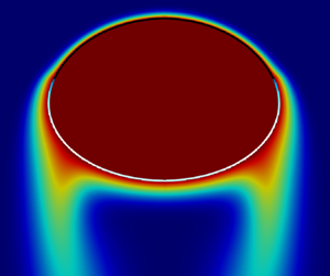
Velocity fields and surfactant distribution along the interface are plotted in figures 4(a) and 4(b), which correspond, respectively, to Case 7 at  $Ma = 0.7$ and Case 3 at $Ma = 2$. The insoluble surfactants are convected to the rear of the bubble, creating a surface tension gradient which induces Marangoni stresses along the interface: at equilibrium, in the final state of the simulations, the presence of the angle of contamination $\theta _{cap}$ is evidenced, which sharply separates areas with slip and no-slip condition at the interface. This state is referred to a partial interface immobilisation, for which the volume and intensity of the circulation inside the bubble is reduced.

Figure 4. Velocity field: (a) Case 7 ( $Re = 23.4$, $Ma = 0.7$, $\theta _{cap} = 1.68$, $\chi = 1.61$); (b) Case 3 ( $Re = 53.0$, $Ma = 2$, $\theta _{cap} = 1.36$, $\chi = 1.45$).
The bubble shapes reported in these two figures are typical of what is observed in the present simulations. One can notice that the rear of the bubble is flatter in figure 4(a), presenting a larger asymmetry between the two halves than in figure 4(b). This is generally different from what is observed with clean oblate bubbles at comparable Weber number, which are always more flattened in the front part, as shown in Aoyama et al. (Reference Aoyama, Hayashi, Hosokawa and Tomiyama2016). Here, the presence of surfactants, which accumulate at the rear, makes the surface tension locally decline, which results in an increase of deformability of this part of the interface.
In the wake, the onset of a recirculation is barely noticeable in figure 4(b), since  $Re$ is higher. Let us comment on the conditions where such a flow separation occurs. In the case of a fully immobile interface, a translating sphere presents a circulation in its wake when $Re \geq 20$ (Johnson & Patel Reference Johnson and Patel1999). In the opposition condition of a mobile interface, a standing eddy is present only provided that the bubble distortion is sufficient, for instance for an aspect ratio larger than $2.2$ at $Re = 20$ and larger than 1.7 at $Re = 60$ (Blanco & Magnaudet Reference Blanco and Magnaudet1995; Magnaudet & Mougin Reference Magnaudet and Mougin2007). In intermediate interface mobility cases, the ability of surfactants to control the wake at the trailing edge has been shown by Wang, Papageorgiou & Maldarelli (Reference Wang, Papageorgiou and Maldarelli2002) for spherical bubbles, and depends on the $\theta _{cap}$ value in the stagnant-cap regime (Dani et al. Reference Dani, Cockx, Legendre and Guiraud2022). In the present simulation cases with distorted bubbles, we observe the same: surfactants are able to make appear a standing eddy in the bubble wake in cases where the latter should not be present in condition of a fully mobile interface, which is for instance the case in figure 4(b). It is interesting to note that a very small surface concentration (i.e. a small portion of the interface with no-slip condition) can be sufficient to allow a circulation to develop. The only condition for which recirculation is not observed in the present study corresponds to the case where both the bubble remains very close to a sphere ( $\chi \leq$1.2) and its Reynolds number is smaller than 20 (as in Case 5).
Profiles of the tangential velocity  $u_s$ and the surfactant concentration $\varGamma$ along the bubble surface are plotted in figure 5 for Case 3, at $Ma = 0.7$. The velocity is zero at the stagnation point $\theta = 0$, then increases and finally drops to zero at the contamination angle ( $\theta = \theta _{cap}$). A strong gradient of $\varGamma$ is observed at this point, where the Marangoni stresses are therefore the highest. At the rear of the bubble, the surfactant distribution does, however, not evolve monotonically since a weak decrease is observed towards the south pole: this is the signature of the recirculation zone in the bubble wake, which convects surfactants in the opposite direction of the downward liquid flow due to the rise motion, making them to accumulate around $\theta \approx 5{\rm \pi} /8$ (where $\varGamma$ is maximal). However, for cases where no recirculation zone is present in the bubble wake, the maximal surface concentration value is still found at $\theta = {\rm \pi}$.

Figure 5. Profiles of normalised fluid velocity  $u_{s} / U_{\infty }$ at the interface, and surfactant concentration $\varGamma$ normalised by the average concentration $\bar {\varGamma }$, along the polar angle $\theta$, for Case 3 at $Ma = 0.7$. Here $\theta = 0$ and $\theta = {\rm \pi}$ correspond, respectively, to the apex and the rear of the bubble.
In figure 6(a,b), for the different cases, the evolution of the Reynolds number and the aspect ratio are shown when increasing the Marangoni number, i.e. decreasing the contamination angle  $\theta _{cap}$, from the clean case ( $\theta _{cap} = 0$) to the fully contaminated condition ( $\theta _{cap} = {\rm \pi}$). The Reynolds number is divided by the clean reference $Re^{clean}$ obtained, when $Ma = 0$ at same $Ar$ and nearly constant $Eo$ (note that the bubble aspect ratio is not conserved in these different conditions, as in an experimental configuration).

Figure 6. Evolution of the Reynolds number and the aspect ratio from a clean to a fully contaminated interface at different  $Ar$, depending either (a,b) on the contamination angle $\theta _{cap}$ or (c,d) on the portion of the surface $S^{*}(\theta _{cap})$ which is surfactant-free (or mobile).
It is observed that the ratio  $Re / Re^{clean}$ declines while the coverage rate of the interface increases, for each case. It can be emphasised that, once $\theta _{cap}$ is lower than ${\rm \pi} /2$, the bubble velocity changes very slowly, being close to its minimal value (the same as for a spheroidal particle of same aspect ratio). However, surprisingly one can notice that the larger the bubble distortion, the smaller the decrease of $Re / Re^{clean}$: the curves of the different cases are ordered according to the value of the aspect ratio, by comparing figure 6(a,b). For Case 4, the rise velocity seems even unaffected by contamination, by a change of only $\pm 5\,\%$ between the different $\theta _{cap}$ conditions, at the same $(Ar, Eo)$; surprisingly, for this case, $Re$ is even slightly larger than $Re_{clean}$ for some $\theta _{cap}$ values. To understand this observation, let us remember that a crucial parameter is not conserved here, when comparing the bubble velocity with or without surfactants: the distortion of the bubble changes, as there is a strong interplay between the rise velocity, contamination and the aspect ratio. For each case, figure 6(b) reveals that when the bubble is progressively contaminated, $\chi$ declines. Actually, the evolution of $Re$ for a bubble in the presence of surfactants is the result of competing effects: (i) as a contaminated bubble has a partially immobile interface, it rises slower than a clean bubble of same size (the drag force is increased), leading to a smaller Weber number – the decrease of dynamic pressure responsible for the bubble distortion is much larger than the reduction of the average surface tension due to the surfactants – so, consequently a smaller bubble distortion is obtained; (ii) this smaller deformation reduces the drag between the liquid and the bubble, which tends in turn to mitigate the velocity decline compared with the clean case. Such competing effects explain the unusual observation on Case 4, of a close or slightly larger velocity for the contaminated bubble compared with the clean one. This result will be further discussed in § 4.2.2.
Regarding the bubble deformation evolution, when increasing the contamination,  $\chi$ first slightly decreases, then strongly drops while $\theta _{cap}$ approaches the equator. However, once the latter is crossed for $\theta _{cap}$, the aspect ratio becomes surprisingly constant, whatever the location of the contamination angle and for all the cases in terms of $(Ar, Eo)$. One can therefore observe that the hydrodynamic behaviour of the bubble evolves significantly when the cap angle is in the southern hemisphere, whereas the main quantities are fixed once it is in the northern one.
To properly analyse such a strong coupling between the rising velocity, interface contamination and bubble deformation, it is required to work with dimensionless quantities such as the drag coefficient, which is the object of the next section.
An alternative plot is introduced in order to better compare the behaviour of oblate bubbles of different aspect ratios: evolutions of the rise velocity and the aspect ratio are presented as a function of the portion of the interface which is surfactant-free (i.e. mobile), rather than  $\theta _{cap}$. In this way, the percentage of mobile surface $S^{*}(\theta _{cap})$ is introduced, hence $S^{*}=1$ when the interface is clean whereas $S^{*}=0$ when the bubble is fully covered by surfactants. At a given $\theta _{cap}$, the $S^{*}$ function directly depends on the bubble shape. Figure 6(c,d) show $Re / Re^{clean}$ and $\chi$ depending on the surface ratio $S^*$. For instance, for cases at high $\chi$, such as Cases 3 and 7, it can be seen that $Re/Re_{clean}$ drops in a narrow range of $\theta _{cap}$ (figure 6a) whereas, when plotting this curve along $S^{*}(\theta _{cap})$, the evolution is not so abruptly centred around $\theta _{cap} = {\rm \pi}/2$. In the same way, the evolution of the aspect ratio is smoother when plotted as a function of $S^*$. The sudden decrease of $Re/Re_{clean}$ or $\chi$ is therefore a bias induced by a different distribution of the surface of the interface, depending on the bubble flatness. The parameter $S^{*}$ will be further used to quantify the drag coefficient variation when the interface is partially immobilised.
4.2.2. Drag coefficient
In the same way as it was proposed for a spherical bubble by Sadhal & Johnson (Reference Sadhal and Johnson1983), we define the reduced drag coefficient for an oblate bubble as
 \begin{equation} C_{D}^{*} (Re, \chi) = \frac{C_{D} - C_{D}^{clean} (Re, \chi)}{C_{D}^{solid} (Re, \chi) - C_{D}^{clean} (Re, \chi)} , \end{equation}
where  $C_{D}^{clean}$ and $C_{D}^{solid}$ are given by the correlations selected in the validation section, (4.6) and (4.9), respectively. For all the cases, figure 7 reveals that the $C_{D}^{*} (Re, \chi )$ values lead to a master curve when plotted as a function of surfactant-free surface ratio $S^{*}$. Note that the collapse is much better when using $S^{*}$ instead of $\theta _{cap}$ in the abscissa, whereas both representations are equivalent for spherical bubbles. Thus, it is found that the evolution of the reduced drag coefficient is startlingly similar whatever $Re$,
$Re$,  $\chi$ and $Ma$. It is confirmed on this plot that the bubble velocity is close to its minimal value ( $1 \geq C_D^{*} \geq 0.75$) provided that half of the interface is immobile $S^{*} \leq 0.5$. The analytical expression given by Sadhal & Johnson (Reference Sadhal and Johnson1983) for spherical bubbles in the Stokes regime is shown for comparison, being plotted by associating the $\theta _{cap}$ value in the original expression with the corresponding $S^{*}(\theta _{cap})$ computed on a sphere. This analysis points out that the evolution of the reduced drag coefficient of an oblate bubble can be estimated with good accuracy by using the same expression as for spherical bubbles, provided that the $S^{*}$ function is introduced. From a practical point of view, it enables a direct estimation of the stagnant-cap angle (with interest for mass transfer rate prediction for instance, as shown in the section dedicated to that point) when both the bubble velocity and its aspect ratio are measured: $C_D^*$ can be calculated, allowing to deduce $S^*$ thanks to the expression of Sadhal & Johnson (Reference Sadhal and Johnson1983) (figure 7), then to predict $\theta _{cap}$ by using a geometrical relationship on an oblate shape of known $\chi$.

Figure 7. Reduced drag coefficient  $C_{D}^{*}$ depending on the contaminated surface $S^{*}(\theta _{cap})$. The results are compared with the expression given by Sadhal & Johnson (Reference Sadhal and Johnson1983) evaluated on a sphere. Note that the points at $\theta _{cap} = {\rm \pi}$ are set to 0 to avoid data scattering for the $C_D^{*}$ of clean bubbles.
The coupling between velocity, partial interface immobilisation, and shape is now analysed. It has been emphasised in figure 6 that, by considering  $Ar$ constant, and progressively increasing $Ma$,
$Ma$,  $Re$ decreases compared with the case at ${Ma=0}$, the decrease being less important for a highly distorted bubble. For a better understanding, the force balance on the bubble at equilibrium is considered: the drag force $\tfrac {1}{2} \rho _{liq} U_{\infty }^{2} {\rm \pi}({d_{eq}^{2}}/{4}) C_{D}(Re, \chi )$ balances the buoyancy force $(\rho _{liq} - \rho _{gas}) g {\rm \pi}({d_{eq}^{3}}/{6})$. Therefore, the following relationship is established:
 \begin{equation} \quad Re = \sqrt{\frac{4}{3} \frac{1}{C_{D}(Re,\chi)}} \sqrt{Ar} . \end{equation}
Note that, in (4.15), the effect of surfactants on the bubble dynamics is accounted for by the expression used for  $C_{D}$, which depends on the interface mobility. At constant $Ar$, when considering the presence of surfactants at an interface which induces Marangoni stresses, two competing phenomena occur with opposite effects on $C_D$, based on figure 6: (i) the interface becomes (partially) immobilised, making $C_{D}$ increase; (ii) the bubble deformation decreases, thus making $C_{D}$, which also depends on $\chi$, decline. Finally, the dimensionless force balance, (4.15), shows that the consequence on $Re$ is directly related to the dominant effect in the variation of $C_D$. For most of the cases presented here, $C_D$ finally increases with $Ma$, as the result of these two competing effects. However, an outstanding case is that of Case 4: its rise velocity is unaffected by the presence of adsorbed surfactants. Indeed, the Reynolds number of the contaminated bubble remains close to that of the clean bubble of the same size whatever $\theta _{cap}$ (figure 6a). The decrease in bubble distortion before and after contamination is therefore so significant that it is able to compensate the increase of $C_D$ due to the interface immobilisation. For this case, the drag coefficients $C_{D}$ for the different $\theta _{cap}$ values are plotted only as a function of $\chi$ in figure 8 (since $Re$ is nearly constant), and are computed from both the simulations and the predictions of (4.6) and (4.8) for the extreme cases of fully mobile and immobile interface, respectively.

Figure 8. Drag coefficient  $C_{D}$ depending on the aspect ratio $\chi$ from (4.6) (red solid line) and (4.8) (blue solid line), evaluated at $Re = 60$. Red and blue symbols correspond, respectively, to $\theta _{cap} = {\rm \pi}$ and $\theta _{cap} = 0$, and white symbols correspond to intermediate $\theta _{cap}$, for Case 4.
It can be concluded from this plot that  $C_{D}$ remains similar whatever $\theta _{cap}$, because both $\chi$ and the interface immobilisation are changing simultaneously. Equation (4.15) justifies that this compensation is consistent with the result of a nearly constant $Re$ for all the flow conditions of Case 4. The evolution of $Re$ with contamination, shown in figures 6(a) or 6(c), is correlated to that of $C_D$ given in figure 8: for Case 4, the slight non-monotonic evolution of $Re$ when increasing the coverage rate of the interface is similar on both representations. Therefore, the dimensionless force balance, given by (4.15), constitutes a solid basis to interpret the evolution of the bubble velocity for contaminated bubbles by including the interplay between the different effects induced by the presence of surfactants.
4.2.3. Marangoni stresses
To analyse the intensity of the Marangoni effect along the interface, a local Marangoni number is introduced, as in Piedfert et al. (Reference Piedfert, Lalanne, Masbernat and Risso2018), as a function of the polar angle  $\theta$:
 \begin{equation} Ma_{loc}(\theta) = \frac{ \| {\boldsymbol{\nabla}_{s} \sigma} \|}{\mu_{liq} \frac{U_{\infty}}{R}} . \end{equation}
Here  $Ma_{loc}$ compares the magnitude of the local surface tension gradient with the viscous stress at the interface, and $Ma_{loc}$ is maximum around the contamination angle $\theta _{cap}$ where the viscous dissipation is the highest, as pointed out by Piedfert et al. (Reference Piedfert, Lalanne, Masbernat and Risso2018), except for fully immobile interfaces where the maximum is reached around ${\rm \pi} /4$. For all the cases, figure 9 reports the maximal value of $\max (Ma_{loc})$ at the surface of each oblate bubble, as a function of the contamination angle. When increasing contamination, i.e. increasing $Ma$ and decreasing $\theta _{cap}$, the Marangoni stress intensity does not monotonically increase. Indeed, as $\theta _{cap}$ decreases from ${\rm \pi}$, (by reading figure 9 from right to left), $\max (Ma_{loc})$ first increases until reaching its highest value when $\theta _{cap}$ is at the equator, then drops at a non-zero value while $0 \leq \theta _{cap} \leq {\rm \pi}/2$. It is remarkable to note that this evolution is the same whatever the case and the bubble deformation, and that the maximal gradient is always reached for the case at which $\theta _{cap} = {\rm \pi}/2$. Indeed, the balance of the tangential stress at the interface yields
 \begin{equation} \left. \mu_{liq} \frac{\partial u_{s}}{\partial n} \right|_{liq} \approx \| {\boldsymbol{\nabla}_{s} \sigma} \|, \end{equation}
since the viscosity ratio is large for a gas bubble leading us to neglect the tangential stress on the gas side. By using the potential flow prediction around an oblate spheroid,  $({\partial u_{s}}/{\partial n}) \sim ({U_{pot} (\theta _{cap})}/{\delta })$, where $U_{pot}$ is the potential flow velocity, taken at $r = R$ and $\theta = \theta _{cap}$, corresponding to the velocity outside the boundary layer and $\delta$ its thickness. Therefore,
 \begin{equation} \max(Ma_{loc}) \sim \frac{U_{pot}(\theta_{cap})}{U_{\infty}} \frac{R}{\delta}. \end{equation}
In the case of an oblate spheroid of aspect ratio  $\chi$, the theoretical calculation of Favelukis & Hung Ly (Reference Favelukis and Hung Ly2005) shows that the maximal value of $U_{pot}$ is located at $\theta = {\rm \pi}/2$ whatever the aspect ratio. Therefore, the scaling given by (4.18) permits us to justify that the Marangoni stresses at the surface of a contaminated bubble are maximal in the case where $\theta _{cap}$ is at the equator. In the stagnant-cap regime, it can be concluded that the intensity of the surface tension gradient does not always increase with the adsorbed surfactant concentration, but its magnitude is strongly sensitive on the $\theta _{cap}$ value.

Figure 9. Maximal intensity of the Marangoni stress along the interface, max $(Ma_{loc})$, depending on the contamination angle $\theta _{cap}$.
4.2.4. Aspect ratio
The bubble shape results from the balance between dynamic and capillary pressures. The analysis from figure 6 has already revealed that a contaminated bubble is less distorted than a clean bubble, for cases at a given  $Ar$ and same $Eo$ (same bubble size and liquid properties, but not the same rise velocity). Besides, it has been emphasised from the simulations of the present study that $\chi$ declines when $\theta _{cap}$ is located in the southern hemisphere ( $\theta _{cap} \leq {\rm \pi}/2$) but, surprisingly, no longer evolves when $\theta _{cap}$ lies in the northern hemisphere. From these results, it has been observed that predictions of $\chi$ from experimental correlations valid for clean bubbles (such as that of Legendre et al. (Reference Legendre, Zenit and Rodrigo Velez-Cordero2012) as a function of both $We$ and $Mo$), overestimate the aspect ratio of a contaminated bubble: the decrease of $We$, due to interface contamination, is not enough to account for the lower deformation compared with a clean bubble at same $(We,Mo)$. Indeed, different experimental correlations exist in the literature to predict the shape of clean or fully contaminated bubbles. Among them, those of Aoyama et al. (Reference Aoyama, Hayashi, Hosokawa and Tomiyama2016) ((4.12) for mobile interfaces) and Aoyama et al. (Reference Aoyama, Hayashi, Hosokawa and Tomiyama2018) ((4.13) for immobile interfaces) constitute a convenient basis of analysis since both are formulated with the couple $(Re, Eo)$.
In order to separate the contribution of these two parameters, the evolution of (i)  $\chi$ as a function of $Eo$ when $Re$ is almost constant (Case 4) is plotted in figure 10(a), and (ii) $\chi$ as a function of $Re$ when $Eo$ barely evolves (Case 2) is plotted in figure 10(b). The theoretical predictions for the extreme cases in terms of interface mobility are also given. From these two figures, one can observe that when ${\rm \pi} /2 \leq \theta _{cap} \leq {\rm \pi}$, the aspect ratio drops from that of clean bubbles to that of a fully contaminated interface, the latter being already reached as soon as $\theta _{cap} \approx {\rm \pi}/2$. Hence, the aspect ratio of a bubble of which the contamination angle is lower than ${\rm \pi} /2$ can be accurately predicted by the correlation for fully immobile interfaces (4.13). The slope of $\chi$ as a function of $Eo$ is 0.3 while it is of 4.3 as a function of $Re$, which means that the variations of the aspect ratio are mostly correlated to those of the Reynolds number. This is consistent with the observation that the bubble velocity is nearly constant once $\theta _{cap}$ lies in the northern hemisphere.

Figure 10. (a) Aspect ratio  $\chi$ depending on the Eötvös number $Eo$ for Case 4 where $Re$ is almost constant. Brown symbols correspond ${\rm \pi} /2 \leq \theta _{cap} \leq {\rm \pi}$. Note that for sake of readability, white colour is used here to illustrate points where $0 \leq \theta _{cap} \leq {\rm \pi}/2$. Red and blue solid lines are calculated from, respectively, (4.12) and (4.13). (b) Aspect ratio $\chi$ depending on the Reynolds number $Re$ for Case 2 where $Eo$ is almost constant. Black and green symbols corresponds, respectively, to $0 \leq \theta _{cap} \leq {\rm \pi}/2$ and ${\rm \pi} /2 \leq \theta _{cap} \leq {\rm \pi}$. Red and blue solid lines are calculated from, respectively, (4.12) and (4.13).
With the objective to explain the evolution of  $\chi$ depending on the location of $\theta _{cap}$, the pressure distribution around the bubbles is now analysed: the pressure difference $\Delta P = P_{A} - P_{E}$, between the apex (A, of pressure $P_A$ in the liquid side) and the equator (E, of pressure $P_E$ in the liquid side), is the main deforming stress due the outer flow (with $P_A > P_E$). The viscous normal stress contribution is not taken into account in the present analysis since it has been verified that its difference between $\theta = 0$ and $\theta = {\rm \pi}/ 2$ is negligible compared with $\Delta P$.
For Case 2, the dimensionless pressures  $P_{A}^{*}$ and $P_{E}^{*}$, normalised by $1/2 \rho _{liq} U_{\infty }^2$, are plotted for different $\theta _{cap}$ in figure 11(a). In the region where ${\rm \pi} / 2 \leq \theta _{cap} \leq {\rm \pi}$, both $P_{A}^{*}$ and $P_{E}^{*}$ vary. In particular, even $P_{A}^{*}$ drops whereas A is located far from $\theta _{cap}$, i.e. the region where the fluid velocity vanishes: the abrupt deceleration that occurs at $\theta = \theta _{cap}$ in the southern zone also impacts the velocity and pressure fields at the apex. The normalised pressure difference between A and E, $\Delta P^{*}$, is shown in figure 11(b). Note that the resisting stress to deformation related to surface tension, $\bar {\sigma } / d_{eq}$, is nearly identical when varying contamination in this case. When $\theta _{cap}$ decreases, provided that it is located in the southern hemisphere, it is found that $\Delta P^{*}$ also declines. This evolution therefore enables us to understand that the bubble is less distorted, while its interface is partially mobile. The Bernoulli principle between A and E, applied here by neglecting the pressure loss along the interface streamline, justifies this decline. Indeed, it leads to
 \begin{equation} \Delta P^{*} = \left(\dfrac{U_E}{U_{\infty}}\right)^2 + \dfrac{\rho_{liq} g \Delta z}{\frac{1}{2} \rho_{liq} U_{\infty}^2}, \end{equation}
where  $\Delta z$ is the height difference between $A$ and $E$. Equation (4.19) predicts that the evolution of $\Delta P^{*}$ when $\theta _{cap}$ varies is related to that of $(U_{E}/U_{\infty })^2$ (the last term due to the variation of hydrostatic pressure between A and E is small and barely evolves). As illustrated in figure 11(b), when $\theta _{cap}$ decreases, $(U_E/U_{\infty })^2$ significantly drops, consistently with the evolution of $\Delta P^{*}$. Thus, provided that $\theta _{cap}$ lies in the southern hemisphere, the dynamic pressure difference inducing the bubble distortion is smaller for a partially mobile interface than for a clean bubble, which is mainly due to the partial decrease of kinetic energy of the fluid at the equator.

Figure 11. Case 2: (a) dimensionless pressure  $P^{*}$ at point $A$ at the front of the bubble, and at point $E$ at the equator, according to the contamination angle; (b) dimensionless velocity $U_{E}$ at the equator at point $E$, and pressure difference $\Delta P^{*} = P_{A}^{*} - P_{E}^{*}$ depending on the contamination angle.
When  $\theta _{cap}$ is in the northern hemisphere, as shown with the reduced drag coefficient, the rise velocity is close to that of a particle with full no-slip condition. For illustration, dimensionless pressure fields $P^{*}$ are presented in figure 12 for Case 3 at $Ma = 2, 4$ and 20 (the latter value being the case of a fully immobile interface), for which $Re$ and $\chi$ are similar. The cap angle is known to be a location where the hydrodynamic conditions abruptly vary (Cuenot et al. Reference Cuenot, Magnaudet and Spennato1997). For instance, at $Ma = 2$ or 4, one can observe an overpressure at $\theta = \theta _{cap}$, as it is a new stagnation point at the interface. Behind $\theta _{cap}$, the interface is immobile and the pressure suddenly decreases: the figure shows that the pressure field around the equator at $Ma=2$ or 4 is similar to the one of a fully immobile interface like for the case $Ma=20$. This region of low pressure corresponds to the location where the velocity is maximal outside the boundary layer. Figure 11(a) confirms that $P_{E}^{*}$ is notably independent of $\theta _{cap}$ when the latter lies in the north pole, and reveals that $P_A^{*}$ also barely evolves with $\theta _{cap}$. Therefore, a constant $\Delta P^{*}$ is reached (figure 11b), which is smaller than for cases where $\theta _{cap}$ lies in the south pole. Finally, for cases where $\theta _{cap} \leq {\rm \pi}/2$, the dimensionless pressure stress, due to the outer flow and causing the bubble distortion, is shown to be independent of $\theta _{cap}$ because some of the flow features, $P_{A}^{*}$ and $P_{E}^{*}$, are sufficiently close to those around an oblate solid sphere despite the remaining interface mobility between A and E, allowing us to understand that $\chi$ is matching the prediction for fully immobile interfaces in that case.

Figure 12. Case 3: dimensionless pressure  $P^{*}$ field and dimensionless interface velocity $u_{s}^{*}$ (normalised by the maximal tangential velocity of each case), at different Marangoni numbers where the stagnant-cap angle lies in the northern hemisphere.
To rationalise these different evolutions, a general correlation is proposed for the aspect ratio  $\chi ^{cont}$ of contaminated bubbles, whatever the $\theta _{cap}$ location, in the form
 \begin{equation} \chi^{cont} = (1 - \alpha) \chi^{solid} + \alpha \chi^{clean}, \end{equation}
where  $\alpha$ is given by
 \begin{equation} \alpha = (1 - {{C_{D}}^{*}}^{2.5})^{5}. \end{equation}
This correlation describes the transition of the aspect ratio from that around a bubble with mobile interface, provided by (4.12), to that around a bubble with fully immobile interface, provided by (4.13), considering  $C_D^{*}$. The large exponent used in (4.21) is employed to figure out that $\alpha$ becomes negligible when $\theta _{cap} \leq {\rm \pi}/2$, i.e. $C_D^{*} \geq 0.75$, leading to aspect ratios close to the limit of fully immobile interfaces. A parity curve is displayed in figure 13 for all the numerical data provided in this study, and a good matching is observed between the numerical simulations and the proposed correlation, with a discrepancy below 10 % for these oblate contaminated bubbles with aspect ratios until 3. In this way, the correlation (4.20), is able to explain the variations of the bubble aspect ratio $\chi$ (figure 6b,d) when the contamination rate increases (this also stands for the slight non-monotonic evolution of $\chi$ visible in Case 4 while $\theta _{cap}$ decreases, for which $Re$,
$Re$,  $Eo$ and $C_D^*$ slightly vary between the different $\theta _{cap}$ values).

Figure 13. Parity curve to compare the obtained aspect ratios of contaminated bubbles of all cases with (4.20).
5. Results on the mass transfer rate
For each case, by considering different interface contamination levels, the external mass transfer of a solute from the gas to the liquid is computed, from  $Sc = 1$ to 40 for Cases 1 to 3, and $Sc = 1$ to 100 for Cases 5 to 7. The range of variation of $Sc$ is defined in order to maintain enough mesh points in the thin mass boundary layer which develops around the bubble, to enable an accurate resolution.
In this section, the dimensionless mass flux rate is computed in the form of a global Sherwood number, defined with  $d_{eq}$ as the characteristic length scale,
 \begin{equation} Sh = \frac{d_{eq}}{D (C_{int}-C_{\infty})} \frac{1}{S} \iint_{S} - D \boldsymbol{\nabla} C \boldsymbol{\cdot} \boldsymbol{n} \, \mathrm{d}S . \end{equation}
The local Sherwood number,
 \begin{equation} Sh_{loc} = \frac{- d_{eq} \boldsymbol{\nabla} C \boldsymbol{\cdot} \boldsymbol{n}}{(C_{int}-C_{\infty})} , \end{equation}
is also introduced for an analysis of the local values of the mass flux along the interface.
First,  $Sh$ is analysed for clean oblate bubbles, and compared with existing works. Then, results for a contaminated interface are presented.
5.1. Validation: mass transfer around a clean bubble
The results of  $Sh$ for oblate clean bubbles are shown in figure 14. The spatial convergence has first been verified in table 4 where cases at the highest Péclet number $Pe = U_{\infty } d_{eq} / D$ of the present study are listed. The numerical results are properly converged for the mesh $1024 \times 2048$, for $Pe \approx 2500$.

Figure 14. Global and local Sherwood number for clean deformed bubbles. (a) Global Sherwood number  $Sh$ depending the maximum Péclet number $Pe_{max}$. The obtained results are compared with the correlation (5.3) given by Colombet et al. (Reference Colombet, Legendre, Cockx and Guiraud2013). Dashed lines - - correspond to limits $\pm 10\,\%$. (b) Profiles of the local Sherwood number $Sh_{loc}$ along the bubble surface, for Case 3 at $Sc = 30$ and Case 7 at $Sc = 60$.
Table 4. Spatial convergence of the global Sherwood number for a clean deformed bubble ( $\chi \approx 2$), on three different meshes: Case 3 at $Pe \approx 2500$ and Case 7 at $Pe \approx 2400$. Results are compared with (5.3) from Colombet et al. (Reference Colombet, Legendre, Cockx and Guiraud2013).

As mentioned in the introduction, Figueroa-Espinoza & Legendre (Reference Figueroa-Espinoza and Legendre2010) found that the global Sherwood number around a clean ellipsoidal bubble can be reasonably well estimated by the same prediction as for a clean spherical bubble ( $Sh$ is affected by $\chi$ by less than 10 $\%$ at large $Re$). In their work, they compared their results with the calculation from Boussinesq (Reference Boussinesq1905), valid at large $Re$ and $Pe$. In the present study, the correlation given by Colombet et al. (Reference Colombet, Legendre, Cockx and Guiraud2013), later proposed to predict $Sh$ for spherical bubbles whatever $Re$ and $Sc$, is chosen as the reference for the case of a clean interface,
 \begin{equation} Sh^{clean} = 1 + \left[ 1 + \left( \frac{4}{3 {\rm \pi}} \right)^{2/3} (2 Pe_{max})^{2/3} \right]^{3/4} , \end{equation}
where  $Pe_{max}$ is the Péclet number based on the maximum tangential velocity $u_{s \, max}$ of the fluid along the interface. The comparison between this correlation and the obtained Sherwood number is plotted in figure 14(a) for clean bubbles. The numerical results of the present study, with oblate bubbles of aspect ratio $1 \leq \chi \leq 2.1$, $20 \leq Re \leq 60$, $1 \leq Sc \leq 100$ for these cases, are in good agreement with the prediction for spherical bubbles, within 10 % of discrepancy. This conclusion is consistent with the findings from Figueroa-Espinoza & Legendre (Reference Figueroa-Espinoza and Legendre2010), and permits us to validate the numerical resolution of mass transfer.
Profiles of local Sherwood number  $Sh_{loc}$ are plotted in figure 14(b) for Case 3 at $Sc = 30$ ( $Pe \approx 1800$) and Case 7 at $Sc = 60$ ( $Pe \approx 1200$), with bubbles of aspect ratio close to 2. The local Sherwood number is much higher at the front of the bubble ( $\theta \leq {\rm \pi}/ 2$) than at the rear of the bubble. On the contrary to the case of a spherical bubble where the highest value of the mass flux is always located at $\theta = 0$ (see profiles in Kentheswaran et al. (Reference Kentheswaran, Dietrich, Tanguy and Lalanne2022)), for Case 3, the maximal flux position lies just before $\theta = {\rm \pi}/ 2$ due to the deformation, and, for the Case 7, a plateau is noticed in the whole upper part of the bubble. Besides, both configurations present a recirculation zone at the rear of the bubble when $\theta \geq 3 {\rm \pi}/ 4$: the vortex in the wake favours slightly the mass flux at the rear of the bubble. However, it is clear from figure 14(a) that the positive effect of the recirculation on the mass transfer rate does not significantly affect the global $Sh$, which still reasonably follows the same law as for a spherical bubble that does not present any circulation vortex when the interface is fully mobile. This is due to the fact that the major part of the transfer occurs at the front of the bubble, in any case.
Note that the obtained profiles of  $Sh_{loc}$ have similar features to the ones presented by Figueroa-Espinoza & Legendre (Reference Figueroa-Espinoza and Legendre2010) for oblate bubbles at $\chi = 2$, regarding the location of the maximal flux or the presence of a plateau in $Sh_{loc}$ at the front of the bubble, even if they have been obtained at larger $Pe$ than in the present study.
In the next section, results on the mass transfer rate around partially contaminated bubbles are presented.
5.2. Sherwood number around a partially contaminated bubble
The dimensionless solute concentration in the liquid phase and the dimensionless surfactant concentration on the bubble surface are both plotted in figure 15 for Case 7 at  $Ma = 0.7$ and Case 3 at $Ma = 2$, both at $Sc = 10$. The mass boundary layer is again the thinnest in the upper part of the interface, which is free of surfactants. Besides, a sudden increase of the mass boundary layer is noticeable around $\theta _{cap}$, when switching from a mobile to an immobile interface: in the region covered by surfactants where the tangential velocity at the interface is zero, the local mass flux is similar to the one around a solid particle, as shown by Dani et al. (Reference Dani, Cockx, Legendre and Guiraud2021) and Kentheswaran et al. (Reference Kentheswaran, Dietrich, Tanguy and Lalanne2022) in the case of a spherical bubble. At the rear of the bubble, the recirculation vortex contributes to improve mixing of the solute in the bubble wake, making it slightly decrease the thickness of the mass boundary layer around the south pole.

Figure 15. Surface concentration fields of surfactants and of the dissolved solute in the liquid phase at  $Sc = 10$: (a) Case 7 ( $Re = 23.4$, $Ma = 0.7$, $\theta _{cap} = 1.68$, $\chi = 1.61$), (b) Case 3 ( $Re = 53.0$, $Ma = 2$, $\theta _{cap} = 1.36$, $\chi = 1.45$).
A local analysis is proposed based on the profiles of local Sherwood number, plotted in figure 16 for Case 7, at  $Sc = 10$, at different Marangoni numbers, i.e. different $\theta _{cap}$. Previous observations on the concentration fields are confirmed: similarly to a clean oblate bubble, the mass flux is much higher at the upper part of the bubble, and the positive impact of the circulation vortex at the rear is small. Besides, the discontinuity of the mass flux around $\theta _{cap}$ is also clear in these profiles.

Figure 16. Profiles of local Sherwood number  $Sh_{loc}$ for Case 7 at three different Marangoni numbers, at $Sc = 10$. Positions of $\theta _{cap}$ are indicated for both partially contaminated bubbles. Note that bubbles at $Ma = 2$ and $Ma = 20$ are almost at same $Re$ and $\chi$.
An important observation is obtained from comparing the cases at  $Ma=2$ and $Ma=20$: the profiles of $Sh_{loc}$ are noticeably different while $Re$ and $\chi$ are the same (the two $Re$ differ only by 4 $\%$). Moreover, the global Sherwood number between these two cases presents a discrepancy of 33 %. This underlines that the three parameters $Re$,
$Re$,  $Sc$ and $\chi$ are not sufficient to describe the transfer rate around a contaminated bubble, even though they can themselves be affected by the contamination (which is not the case on the example taken here). Therefore, the same conclusion as for spherical bubbles (Kentheswaran et al. Reference Kentheswaran, Dietrich, Tanguy and Lalanne2022) is established: at same $Re$,
$Re$,  $Sc$ and $\chi$, a parameter describing the change in interface mobility must be introduced to quantify $Sh$, based for example on the $\theta _{cap}$ value which is not the same in the cases of figure 16. In this previous study for spherical bubbles, it was proposed to quantify such a modification in the hydrodynamics induced by surfactants by considering the maximum tangential velocity at the interface $u_{max}$, normalised by the value for a clean interface at same $Re$ (given by Legendre (Reference Legendre2007)), leading to the dimensionless ratio $u_{max}^{*}$ which has been shown to be a unique function of $\theta _{cap}$ in Kentheswaran et al. (Reference Kentheswaran, Dietrich, Tanguy and Lalanne2022).
Finally, as the impact of surfactants on the mass transfer flux around a contaminated ellipsoidal bubble presents the same features as for the spherical case, and following the result that, for clean bubbles,  $Sh$ depends very weakly on $\chi$, the global Sherwood number is now compared with the correlation proposed by Kentheswaran et al. (Reference Kentheswaran, Dietrich, Tanguy and Lalanne2022) for spherical contaminated bubbles,
 \begin{equation} Sh^{cont} = 2 + Re^{1/2} Sc^{f(\theta_{cap})} \left[ {u_{max}^{*}}^{1.5} \frac{2}{\sqrt{\rm \pi}} g^{clean} + \left( 1 - u_{max}^{*} \right)^{1.2} g^{solid} \right] - \left(1 - u_{max}^{*} \right)^{1.2}, \end{equation}
with
 \begin{gather} g^{clean} = \left( 1 - \frac{2}{3} \frac{1}{(1 + 0.09 Re^{2/3})^{1.1}} \right)^{0.45} , \end{gather}
 \begin{gather} g^{solid} = Re^{{-}0.09} \left( 1 + \frac{1}{Re \, Sc} \right)^{1/3} , \end{gather}
 \begin{gather} f(\theta_{cap}) = \frac{1}{3} - 0.014 \theta_{cap}^{2} + \frac{1}{\rm \pi} \left(\frac{1}{6} + 0.014 {\rm \pi}^{2} \right) \theta_{cap} . \end{gather}
The dimensionless maximal velocity  $u_{max}^{*}$ at the interface which quantifies the magnitude of the tangential flow along the interface compared with the case of a clean and spherical bubble at same $Re$, and which therefore lies between 0 and 1 as an indicator of the decrease in internal circulation inside the bubble, is given by the following fitting function from Kentheswaran et al. (Reference Kentheswaran, Dietrich, Tanguy and Lalanne2022):
 \begin{equation} u_{max}^{*} = 0.5216 \tanh\left(1.8 \theta_{cap}^{0.85} - \frac{\rm \pi}{2}\right) + 0.4784. \end{equation}
Note that (5.8) has been established in the case of spherical bubbles, and is not modified here to be introduced into (5.4) for sake of simplicity (even though the maximal tangential velocity of the fluid at the interface actually also depends on  $\chi$ for oblate bubbles).
The correlation for  $Sh$, given by (5.4), predicts the transition between the Sherwood number of a clean bubble (Takemura & Yabe Reference Takemura and Yabe1998) and that of a solid particle (Clift et al. Reference Clift, Grace and Weber1978), by having an exponent of the Schmidt number that varies between $1/2$ and $1/3$ (which are the respective values for these two extreme cases), and by using $u_{max}^{*}$ as a weighting parameter of the prefactors from the respective scaling laws of each extreme case.
For the oblate bubbles of this study, the comparison of the prediction from (5.7) with the values from the numerical simulations is shown in figure 17 for our different cases in the range  $20 \leq Pe \leq 2400$, $1 \leq \chi \leq 3$, $0 \leq \theta _{cap} \leq {\rm \pi}$. A good agreement is noted, and a maximal discrepancy of 16 % is present. This result confirms that the correlation proposed in the case of spherical contaminated bubbles (Kentheswaran et al. Reference Kentheswaran, Dietrich, Tanguy and Lalanne2022) is also still surprisingly valid for oblate bubbles in a large range of bubble distortion.

Figure 17. Parity curve to compare the obtained global Sherwood number  $Sh$ with the correlation (5.4) (solid line), for Cases 1, 3, 4, 5 and 7. Dashed lines - - correspond to limits $\pm 10\,\%$.
In this way, surfactants impact  $Sh$ for a rising bubble, either spherical or oblate, by affecting both the Reynolds number of the bubble, and the velocity profile in the clean part of the interface ( $u_{max}^{*}$ is decreased) where the mass transfer rate is the highest.
6. Conclusions
In this paper, axisymmetric numerical simulations have been performed to investigate the impact of surfactants on both the interface immobilisation, the bubble deformation and the gas–liquid mass transfer. Such a study has been carried out under the assumption of a stagnant-cap regime, i.e. with insoluble surfactants at a constant mass at the interface, which corresponds to the most common case of a surfactant with slow adsorption/desorption compared with their rate of surface convection. Simulations have been carried out at given  $Ar$, nearly constant $Eo$, and variable $Ma$ leading to different $\theta _{cap}$. Regarding the external mass transfer of a solute from the gas to the liquid, the associated Sherwood number is also analysed, at variable $Sc$.
$Sc$.
For the extreme cases of fully mobile and immobile interfaces, the drag coefficient and aspect ratio have been compared with existing works, with excellent agreement. In particular, for highly contaminated and deformed bubbles (fully immobile interfaces), for which only a few results exist, the present study proves that the experimental correlation of the aspect ratio from Aoyama et al. (Reference Aoyama, Hayashi, Hosokawa and Tomiyama2018) is general since it requires no assumption about the type of surfactant, as suggested by Chen et al. (Reference Chen, Hayashi, Hosokawa and Tomiyama2019).
Regarding partially contaminated bubbles, the reduced drag coefficient  $C_D^{*}$ can still be predicted by the analytical function of Sadhal & Johnson (Reference Sadhal and Johnson1983), even in inertial conditions and for oblate bubbles, provided that it is defined as a function of $S^{*}(\theta _{cap})$, the percentage of surfactant-free surface area, instead of $\theta _{cap}$. The Marangoni stresses do not monotonically increase with the surfactant concentration, but reach a maximal value when $\theta _{cap}$ lies at the equator. It has also been observed that the bubble velocity is very close to that of a solid particle, of same size and aspect ratio, as soon as $\theta _{cap}$ belongs to the northern hemisphere. It has been emphasised that the distortion of a contaminated rising bubble is smaller than that of a clean bubble at same parameters (same couple $(We, Mo)$ or $(Re, Eo)$). The aspect ratio changes significantly with contamination, depending on the stagnant-cap angle position. When $\theta _{cap}$ lies in the southern hemisphere, the dimensionless dynamic pressure causing the bubble deformation is decreasing, as is the kinetic energy of the fluid at the equator (because of the retarded interfacial velocity profile). However, when $\theta _{cap}$ belongs to the northern hemisphere, the pressure difference between the apex and the equator, causing the bubble distortion, becomes constant and is similar to that around a spheroidal particle, which explains that the bubble aspect ratio matches the case of a fully immobile interface. A general correlation, (4.20), is proposed to predict $\chi$ for a contaminated bubble.
Concerning mass transfer, the Sherwood number characterising the external transfer around an oblate bubble can still be predicted with a good accuracy by the same correlation as for a contaminated spherical bubble, (5.4) from Kentheswaran et al. (Reference Kentheswaran, Dietrich, Tanguy and Lalanne2022), for  ${1 \leq \chi \leq 3}$. The bubble distortion does not significantly impact the mass transfer rate, like for oblate clean bubbles at large Reynolds number.
Note that the average surfactant concentration at the interface, involved in the Marangoni number in the present investigation, is generally unknown in practical conditions. However, it can be related to the bulk transport properties of the surfactant. For this purpose, at first glance,  $\bar {\varGamma }$ can be estimated by balancing the adsorption and desorption fluxes of surfactant between the bulk and the interface, assuming equilibrium (Palaparthi et al. Reference Palaparthi, Demetrios and Maldarelli2006; Dukhin et al. Reference Dukhin, Kovalchuk, Gochev, Lotfi, Krzan, Malysa and Miller2015). For instance, the adsorption term can be written in the limit of a uniform bulk concentration of surfactant $C_0$ and by using a linear kinetics (consistently with (2.7)), i.e. assuming an adsorption flux in the form $\beta C_0 \varGamma _{\infty }$ with $\beta$ the adsorption constant and $\varGamma _{\infty }$ the maximum packing concentration, while the desorption rate is expressed as $\alpha \bar {\varGamma }$ with $\alpha$ the desorption constant; it results that $\bar {\varGamma }/\varGamma _{\infty } = \beta C_0 / \alpha$ under these assumptions. Such an expression provides an estimate for $\bar {\varGamma }$ in steady state, allowing us to compare with the numerical results from this study. Note also that the present simulations could be extended by considering the mass exchange processes of soluble surfactants between the bulk and the interface, as a perspective, with the aim of analysing the dynamics of bubble distortion during its progressive contamination (transient evolution for $\bar {\varGamma }$).
Conversely, the results provided here offer a way to evaluate the level of contamination of the surface of a distorted bubble, through the measurement of several parameters related to the bubble dynamics (rise velocity, aspect ratio, rate of bubble dissolution) since they are differently impacted by the presence of adsorbed surfactants.
For instance, one can wonder about the presence of residual contaminants adsorbed at the surface, which weakly affect the surface tension but are sufficient to partially or fully immobilise the interface (Lalanne et al. Reference Lalanne, Masbernat and Risso2020). In that case, the present work shows that the rise velocity is generally reduced compared with the case of a clean interface, but not systematically, contrary to the case of spherical bubbles: it is possible that a contaminated bubble rises at same velocity as a clean one of same size, because the presence of adsorbed surfactants induces a smaller distortion. As the drag coefficient is both increased by a partial immobilisation, and reduced when the bubble is less deformed, these two competing phenomena can compensate in some cases. Therefore, in the case of an ellipsoidal rising bubble, a measurement of the sole rise velocity is not sufficient to conclude on a possible interface contamination, but it is also required to analyse the aspect ratio. Besides, the rate of mass transfer during gas dissolution is smaller for a contaminated bubble than around a clean bubble. However, as a matter of consequence of the previous remark that the bubble Reynolds number may not be affected by contamination, the impact of surfactants on mass transfer around an oblate bubble will be smaller than around a sphere, based on (5.4) which rationalises the evolution of the Sherwood number whatever the contamination degree.
Finally, the simultaneous measurement of different parameters and comparisons to the correlations provided in this study offers a way to conclude on the possible contamination of a bubble interface, in the case of an oblate bubble rising with axisymmetric path.
Acknowledgments
The authors thank Professor O. Masbernat and Dr S. Tanguy for fruitful discussions on the results.
Funding
This work was granted access to the HPC resources of CALMIP supercomputing center under the allocations 2021-[P19066] and 2022-[P19066].
The authors would like to acknowledge the financial support provided by Région Occitanie. This research was carried out in collaboration with the FERMaT federation.
Declaration of interests
The authors report no conflict of interest.
Appendix. Numerical data
The following tables 5–11 present the parameters of all simulations that consider the presence of insoluble surfactants adsorbed at the bubble surface, for each case described in table 1 in their reference state with a clean interface.
Table 5. Case 1.

Table 6. Case 2.

Table 7. Case 3.

Table 8. Case 4.

Table 9. Case 5.

Table 10. Case 6.

Table 11. Case 7.


