


1. Introduction
The surface of young sea ice is covered by a thin, highly saline layer of slush. The presence of this moist surface layer is frequently mentioned in the journals of early explorers and scientists working in both Arctic (Reference VrangelVrangel’, 1840; Reference De LongDe Long, 1883; Reference GreelyGreely, 1886; Reference CollinsonCollinson, 1889; Reference Malmgren and SverdrupMalmgren, 1927) and Antarctic (Reference ScottScott, 1905; Reference Arctowski and BelgicaArctowski, 1908; Mawson, 1909; Reference Wright and PriestleyWright and Priestley, 1922) regions, and has been known to the indigenous peoples of the Arctic for centuries (Reference NelsonNelson, 1969). However, references to such a surface layer in modern scientific literature are rare, largely due to the standard technique of measuring sea-ice salinity profiles, whereby cores are cut into 0.05–0.10 m sections and fail to show the finer detail of the profile near the surface (Reference MartinMartin, 1979), and to the general paucity of field studies on thin ice during winter. Reference MartinMartin (1979) measured salinities on newly formed sea ice in the Beaufort Sea as high as 95%, while Crocker (unpublished) found salinities on fast ice in Resolute Passage, N.W.T., as high as 110%, and on leads in the Arctic Ocean up to 150%. As the ice thickens, frost flowers (a form of hoar frost) begin to appear on its surface and, gradually increasing in size and number, can develop into a continuous snow cover without mass inputs from blowing or falling snow. The frost flowers contain considerable quantities of salt and through capillary suction draw additional brine from the surface, resulting in a highly saline snow cover (particularly in the near-surface layers) containing large amounts of liquid even at very low temperatures. Normally, within 1 or 2 weeks of formation, the structure of the frost-flower layer is modified by strong winds, often accompanied by falling or drifting snow, and constructive and destructive metamorphosis, but it maintains some of its original characteristics, most importantly the high brine volume.
Although comprising only a few centimetres, this moist snow layer is by no means insignificant. The wetness and high salinity affect heat and vapour transfers (Reference Ono and KasaiOno and Kasai, 1985), the reflectivity and emissivity of the ice (Reference Ramseier, Gloersen, Campbell, Chang, Kondrat’yev, Rabinovich and NordbergRamseier and others, 1975; Reference GrenfellGrenfell, 1986; Reference Lohanick and GrenfellLohanick and Grenfell, 1986), and brine drainage and air-bubble patterns during spring melting (Reference MartinMartin, 1979). Despite this, measurements of snow-cover salinities are rare. Spot measurements have been reported by Reference MartinMartin (1979), and some time-series data can be found in Lapp and Prashker (unpublished) and Reference TakizawaTakizawa (1985), but to the authors' knowledge the only detailed study of the spatial and temporal variations in snow-cover properties, including brine volume, is that of Crocker (unpublished). The influence of the brine on the thermal conductivity of snow has been modelled by Reference CrockerCrocker (1984), but the presence of brinesoaked snow is also of direct significance to active microwave radar remote-sensing techniques. These data therefore provide us with an opportunity to investigate the dielectric and scattering properties of such surfaces. In the following sections, we present a simple theoretical analysis of the effect of brine on the complex dielectrics of a shallow snow cover, focussing on the effects of temporal variations in the physical and electromagnetic properties of the surface layers upon scattering of incident energy over the microwave range of frequencies. The implications of these changing snow properties for active microwave remote sensing of ice characteristics are investigated.
2. Snow-Cover Properties
The snow-cover data used in this paper are from Crocker (unpublished) and have been summarized in Reference Crocker and LewisCrocker and Lewis (1985). The measurements were made on young sea ice in Resolute Passage, N.W.T., during November and December 1982. Daily averages of snow temperature, density, salinity, and brine volume were computed at 1 cm depth intervals from nine samples taken from a 3 × 3 grid on a uniform fast-ice sheet. Temperatures were measured with a calibrated Fenwal GB32P2 glass probe thermistor and Data Precision model 245 digital multimeter. A purpose-built snow sampler was used to collect known volumes of snow from each layer, which were bagged and returned to Resolute for weighing, and the salinity of the melt determined with a YSI model 32 conductivity meter calibrated against standard ocean water. The ice first began to form on 7 November, and detailed measurements were started on 15 November when the ice was 0.40 m thick and the frost-flower cover had grown sufficiently to be considered a continuous snow cover. Although some measurements of the ice-surface and frost-flower salinities, and the frost-flower density, were made during the first week of ice growth, difficulties in sampling and interpreting the data make them of limited use in the current study. Therefore, only data from 15 November onward will be used here, and the analysis should be considered applicable only to periods when a continuous, frost-flower-based snow cover is present.
From the snow temperature, density, and salinity, the volume fractions of air, pure ice, and brine (the quantities of interest in modelling the snow-cover dielectric properties) can be calculated from the phase relations for sea ice. After measuring the salinity of a melted snow sample and subtracting the proportion of salt which will be in a solid form (the cryohydrates) at the measured snow temperature (see Reference AssurAssur, 1960), the brine volume of the salt/ice mixture can be determined from tables (Reference AssurAssur, 1960) or equations (Reference Frankenstein and GarnerFrankenstein and Garner, 1967). As the densities of brine and ice are different, the brine volume determined in this manner cannot be directly converted to the volume fraction of brine in the snow-pack. First, the weight ratios of brine (Rb) and ice (R i) must be calculated
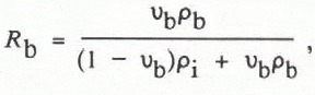
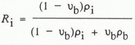
where pi is the density of pure ice, and pb is the density of brine, approximated using
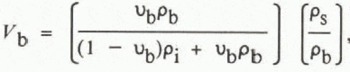
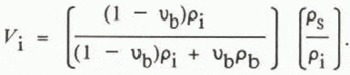
where p0 is the density of pure water, γ is a constant (roughly 10−2), and Tis the temperature in degrees Celsius (Reference Eide and MartinEide and Martin, 1975). The mass of each component is found by multiplying its weight ratio by the snow density (ps), and the true volume fractions of brine (V b) and ice (V b) are found by dividing this mass by the appropriate density giving
The volume fraction of air is then simply
The volume fractions of brine, ice, and air are plotted against snow temperature in Figure 1, for a snow density of 300 kg m−3 and salinity of 40%, values found to be typical of the lowest centimetre of the snow-pack.
The most significant feature of the graph with regard to dielectrics is that the volume fraction of brine remains fairly large down to –22.9°C, when sodium chloride dihydrate begins to come out of solution. Below this temperature, V bfalls off rapidly but some liquid remains in the snow at temperatures below –40°C. It should be noted that the volume fraction of cryohydrates has not been calculated. Removing the appropriate amount of salt from the measured salinity before determining V b has the effect of increasing (1 - V b) and thereby causing a small erroneous increase in V b When modelling the dielectric properties of the snow-pack, this effect is negligible since it is the liquid fraction which is dominant; however, for other uses it may be necessary to calculate the cryohydrate fraction as well.
The volume fractions of air, ice, and brine for the Resolute Passage data are shown in Figure 2. The consistent increase in density with time in layer 2 indicates the presence of constructive metamorphosis and mass transfers from the base of the snow-pack into the upper layers, a feature confirmed by the observation of a thin depth-hoar layer developing at the snow/ice interface. Although V iin the bottom layer also increases slightly, this is primarily the result of reduced brine volumes caused by decreasing surface temperatures as the ice thickens. The relatively high brine fractions, particularly in the lowest layer, are clearly evident as are the increases in V bin all layers between days 24 and 32. The reasons for this increase are not immediately evident, but may be associated with additional brine being drawn up from the surface by increased capillary tension after the input of new, more angular, crystals of wind-blown snow during a storm which occurred on days 23 and 24. It is interesting to see that there is a distinct lag in the brine-fraction increase with distance from the ice surface, indicating that the upward flux of brine is slow, taking about a week to reach layer 3. The gap in the time series in the upper layer represents a period when no snow was present at that level, having been scoured by strong wind.
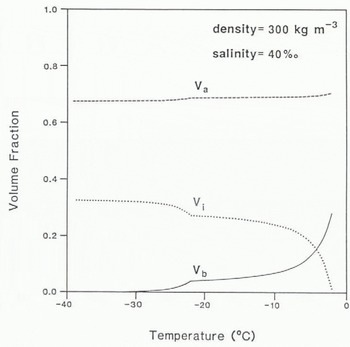
Fig. 1. Variation in the volume fractions of brine (b). ice (i) and air (a) with snow temperature. for a constant snow density of 300 kg m−3 and salinity 40%.
3. Modelling The Dielectric Properties Of Saline Snow
The complex dielectric constant (ε*) of a medium may be represented simply by ε* = ε’ – iε”, where ε’ is the real part of the dielectric constant or permittivity, ε” is the imaginary part or dielectric loss, and i = (–1)1/2. The loss occurring when electromagnetic energy passes through the medium is commonly represented in terms of the loss tangent (tan δ), where tan δ = ε”/ε’.
The snow on young sea ice is a mixture of air, ice, and brine, and its effective complex dielectric constant (ε*) is a weighted average of the complex dielectric constants of the constituent parts. Theoretical studies have shown that the dielectric constant of heterogeneous materials is strongly influenced by the way in which the various components are distributed in the mixture, indicating that any rigorous approach to the problem must include both the dielectric properties of the constituent parts and their distribution. This is the approach adopted here, and we begin by looking at the dielectric properties of ice and saline water.
3.1 Microwave Dielectrics of Ice and Saline Water
Throughout the metre and centimetre wavelength range, the relative complex dielectric constant of ice is invariant (Reference CummingCumming, 1952; Reference EvansEvans, 1965). The real part of the relative complex dielectric constant (εice) is 3.15, and the dielectric loss is so low that it may be ignored (thus, ![]() ). The electromagnetic loss tangent (tan δ) is typically of the order of 10−2 to 10−4, depending on the temperature of the ice, and is several orders of magnitude smaller than the loss tangent of brine. Reference Tiuri, Sihvola, Nyfors and HallikainenTiuri and others (1984) and Reference Hallikainen, Ulaby and Abdel–Razik.Hallikainen and others (1982) found that the relative permittivity
). The electromagnetic loss tangent (tan δ) is typically of the order of 10−2 to 10−4, depending on the temperature of the ice, and is several orders of magnitude smaller than the loss tangent of brine. Reference Tiuri, Sihvola, Nyfors and HallikainenTiuri and others (1984) and Reference Hallikainen, Ulaby and Abdel–Razik.Hallikainen and others (1982) found that the relative permittivity ![]() , the real part of the complex dielectric constant, of dry snow mixtures of air and ice can be represented by the simple linear empirical relationship
, the real part of the complex dielectric constant, of dry snow mixtures of air and ice can be represented by the simple linear empirical relationship
where ![]() is the relative permittivity of dry snow and pdry is its density.
is the relative permittivity of dry snow and pdry is its density.
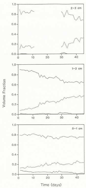
Fig. 2. Variations in the volume fractions of air, ice, and brine for the 46 d observation period in layers 02–1. 1–2. and 2–3 cm measured vertically from the snow/ice interface.
The dielectric behaviour of water as a function of frequency is known in first approximation to conform to a simple Debye relaxation spectrum. The dielectric constant falls off in the dispersion region, whereas the dielectric losses reach a maximum. Salts drastically alter the dielectric loss of water by adding to the free-charge carriers and increasing its conductivity, but the influence on the dielectric constant is small (Reference Hoekstra and CappillinoHoekstra and Cappillino, 1971).
Equations for computing the complex dielectric constant of saline water have been developed by Reference StogrynStogryn (1971), based on an equation of the Debye form, in which the dielectric properties have a salinity and temperature dependence. The term “saline water” is strictly applicable only to water containing Na+ and Cl− ions but, since NaCl is the primary salt in sea-water, Stogryn’s equations for saline water can be used for the brine inclusions in young sea ice and snow without significant error.
To calculate the complex dielectric properties of brine, we have used the following equation (after Reference StogrynStogryn, 1971):
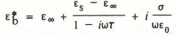
where ![]() is the relative complex dielectric constant of the mixture, and ε∞, εs, ε0, ω, τ, and σ are the high-frequency and static relative dielectric constants of the saline water, the permittivity of free space (i.e. 8.85 × 1O−12farad m−1), the angular frequency, the relaxation time, and the ionic conductivity of the dissolved salts, respectively.
is the relative complex dielectric constant of the mixture, and ε∞, εs, ε0, ω, τ, and σ are the high-frequency and static relative dielectric constants of the saline water, the permittivity of free space (i.e. 8.85 × 1O−12farad m−1), the angular frequency, the relaxation time, and the ionic conductivity of the dissolved salts, respectively.
To obtain values for the parameters in Equation (8), Stogryn developed a series of simple polynomial fits to real dielectric data for saline water, with temperature and salinity as input variables. Results from Stogryn’s equations at a fixed temperature of –2°C and for salinities of 30 and 100% are displayed across the GHz range of frequencies in Figure 3. Reference Vant, Ramseier and MakiosVant and others (1978) discussed these equations and their applicability to the problem of calculating the complex dielectric properties of different sea-ice types.
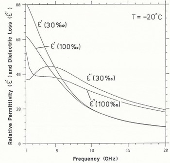
Fig. 3. Behaviour of the relative permittivity ![]() and dielectric loss
and dielectric loss ![]() of brine in the GHz range: measured at salinities of 30% and 100%. and a temperature of –20°C.
of brine in the GHz range: measured at salinities of 30% and 100%. and a temperature of –20°C.
3.1.1. Application of a Mixture Formula
The complex dielectric constant of saline snow (i.e. a mixture of air, ice, and brine) can be determined by a mixing formula which takes into account the specific depolarization due to the liquid inclusions. Interstitial liquid in snow collects around the contact points of the crystals (Reference Drinkwater and InHoltDrinkwater, 1987), forming complex geometric shapes. Although the shape of brine inclusions in the snow matrix does not conform either to perfect ellipsoids or spheroids, Reference DenothDenoth (1980) suggested that, in the case of low liquid fractions, the arrangement of free water may be assumed to approximate to discs. Therefore, the water menisci will be modelled here as oblate spheroids. Reference DenothDenoth (1980) studied snow of varying water content and derived a formula for calculating the specific depolarization factor of liquid inclusions of known dimensions. He also suggested that, as the liquid fraction in a snow cover increases, both the shape of the liquid inclusions and the depolarization factor change. In this paper, however, we discuss only snow of low density and low liquid-volume fractions, and therefore assume that oblate spheroids adequately represent the brine-fraction geometry. A dielectric mixture formula, developed for heterogeneous systems containing dispersed ellipsoids, has been discussed by Reference Beek, van and BirksVan Beek (1967), and a simplified form of this equation, generalized for a uniform distribution of orientations of liquid inclusions in space, was utilized with success by Reference Chaloupka, Ostwald and SchiekChaloupka and others (1980), and more recently by Reference Aebischer and SchandaMätzler and others (1984), for wet snow. Reference Polder van and SantenPolder and van Santen (1946) showed that this type of formulation holds true for low volume fractions of water, and may also accommodate shapes of water inclusions such as those described by Reference DenothDenoth (1980). The formula used to calculate the complex dielectric constant of the mixture ![]() is
is
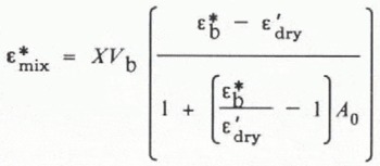
where A
0is the dominant depolarization factor, V
b is the volume fraction of brine, ![]() is complex dielectric constant of brine,
is complex dielectric constant of brine, ![]() is the relative permittivity of dry snow (from Equation (7)), and ί is a coupling factor representing the fraction of brine that can be represented by A
0. For isotropically oriented oblate spheroids, the coupling factor (X)is 2/3. In the case of snow in the pendular regime, Denoth observed a depolarization factor A
0 of approximately 0.053.
is the relative permittivity of dry snow (from Equation (7)), and ί is a coupling factor representing the fraction of brine that can be represented by A
0. For isotropically oriented oblate spheroids, the coupling factor (X)is 2/3. In the case of snow in the pendular regime, Denoth observed a depolarization factor A
0 of approximately 0.053.
The temporal variations in the dielectric properties of the snow cover on young sea ice are modelled using Equation (9), along with the calculated volume fractions of air, ice, and brine from the Resolute Passage data.
3.2. Discussion of Results From Mixture Formula
As temperature, salinity, brine volume, and density vary over the 45 d period (Fig. 2), we see marked changes in the modelled complex dielectrics of the surface snow medium. This is shown in Figures 4 and 5, at 1 GHz (L-band) and 13.6 GHz (Ku-band), respectively, where the gradual evolution of the layer is reflected in the changing electromagnetic properties.
The changes in the imaginary part (ε″) of the relative complex dielectric constant, albeit small, are indicative of the amount of brine in the snow. Although the dielectric loss is slightly larger at higher frequencies, owing to the relaxation mechanism in brine, there is a gradual reduction in ε″ with time over all frequencies.
In direct contrast, the dielectric constant (ε′) is larger at lower frequencies due to large increases in the dielectric constant of brine below 10 GHz (X-band). Generally, ε' increases in the upper 2 cm, tending to the values for dry snow by the end of the observation period. This is due to the continual densification of the snow layer and the decline in brine volumes. The dielectric constant in the layer directly above the saline surface of the frazil, however, shows a small decrease; in this case, the reduction in brine volume dominates over the slight change in density and causes ε' to fall by around 0.5.
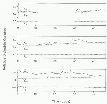
Fig. 4. Predicted variations in ![]() .
. ![]() , and
, and ![]() over the 46 d period. Values are calculated for the snow layers 0–1, 1–2, and 2–3 cm at a frequency of 1 GHz.
over the 46 d period. Values are calculated for the snow layers 0–1, 1–2, and 2–3 cm at a frequency of 1 GHz.
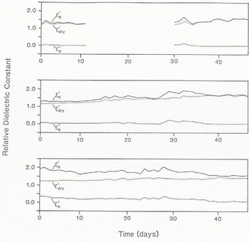
Fig. 5. Predicted variations in ![]() .
. ![]() , and
, and ![]() over the 46 d period. Values are calculated for the snow layers 0–1, 1–2, and 2–3 at a frequency of 13 GHz.
over the 46 d period. Values are calculated for the snow layers 0–1, 1–2, and 2–3 at a frequency of 13 GHz.
In the early part of the measurement period, the difference between the dielectric constants of brine-wetted snow and dry snow will result in increased reflectivity at the air/snow interface. Despite the fact that the mean transmissivity of the snow is generally high (=0.82–0.9), the layer will effectively blanket emission or surface scattering from the saline frazil-ice medium beneath as a result of the high extinction coefficient and lossy nature of saline snow. As time progresses and V b decreases, the snow approaches values observed in higher-density dry snow (εʹ = 1.6 and εʺ = 0.01).
It is clear that the complex dielectric constant of the mixture is largely dependent upon the brine volume and to a lesser extent upon the density of the snow. As brine volume decreases over the observation period, the dielectric properties of the snow cover tend to those of dry snow of similar densities. At lower frequencies, the differences between the relative dielectric constants of brine-wetted snow and dry snow are exacerbated because of the higher dielectric constant of brine.
4. Scattering From Young Ice Surfaces
The radar back-scatter properties of cold, thin first-year ice have been investigated experimentally by Reference Onstott, Moore, Gogineni and DelkerOnstott and others (1982), and in the 8–18 GHz range by Delker and others (1980Reference Delker, Onstott and Moorea, Reference Delker, Onstott and Mooreb), off the Canadian coast at Tuktoyaktuk, N.W.T. The site chosen was a frozen lead, covered with frost flowers of high salinity, a similar situation to that observed in Resolute Passage. Ice-surface temperatures ranged between –20° and –30°C, but a detailed description of the ice or snow densities, surface-roughness properties, snow depth, or snow wetness were unfortunately not given. They observed a strong correlation between radar cross-sections of sea ice and the salinity of the ice surface. In general, higher-salinity thin ice produced higher scattering coefficients than older thicker first-year ice, although the trends of back-scatter coefficient with incidence angle demonstrated parallel responses, i.e. equal angular decays.
Surface roughness is understood to have an important influence on radar scattering from saline-ice surfaces (Reference Kim, Moore, Onstott and GogineniKim and others, 1985), or wet snow surfaces (Reference Stiles and UlabyStiles and Ulaby, 1980). The appearance of any given surface to incident microwave energy may be evaluated using the Rayleigh criterion:
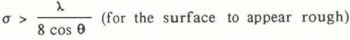
where σ is the standard deviation of surface heights and θ is the incidence angle measured from the normal. The parameters used to describe the snow and ice surfaces are: the standard deviation of small-scale surface height and slope, and the spatial autocorrelation function of the surface, from which the correlation length (l) can be derived. Approximate values derived from close-up photography of early frost-flowered surfaces at the sample site were σ ≃ 0.5 cm and 1 ≃ 5.0 cm. For the frequencies discussed in this study, the snow surface may be considered “rough” for θ > 56° at Ku-band (λ ≈ 2.2cm), θ > 36° at X-band (λ ≈ 3.2 cm), and effectively smooth for all angles at C-band (λ ≈ 5.6 cm) and L-band (λ ≈ 30 cm). Strictly speaking, the separation between specular and diffuse surfaces is not so rigidly defined, and back-scattered energy is almost always distributed over the full range of incidence angles, with a maximum at normal incidence. In addition, the deposition of wind-blown snow changes surface-roughness characteristics throughout the observation period, making characterization difficult without a series of measurements of σ and l.
Kim (unpublished) asserted that surface scattering is liable to be the major back-scattering mechanism for snow-free first-year ice because of the dielectric mismatch between air and a high-salinity ice medium such as frazil ice. The large dielectric constant at the surface of saline ice leads to high reflection coefficients, and thus low trans-missivities or emissivities. At a typical density of 850 kg m−3 and salinity of 4%, the reflection coefficient of frazil ice at normal incidence tends to a minimum of approximately –11.5 dB at temperatures below –40°C, and a maximum of almost 0 dB at 0°C. Several attempts have been made to explain radar back-scatter behaviour for saline ice (Reference Fung and EomFung and Eom, 1982; Kim and others, Reference Kim, Onstott and Moore1984, Reference Kim, Moore, Onstott and Gogineni1985; Parashar, unpublished), all based upon theoretical models of scattering and incorporating work on the physical and electromagnetic properties of ice. Kim (unpublished) demonstrated that physical optics formulations, as reproduced by Reference Ulaby, Moore and FungUlaby and others (1982), can be used to give first-order predictions of the microwave back-scatter of first-year ice. In this paper, we use a similar Kirchoff-type formulation and a “scalar approximation” (Eom, unpublished). The criteria which must be satisfied for the use of such a theoretical model are that the radius of curvature at all points upon the surface are larger than one wavelength, and that the standard deviation of surface heights is small, or of comparable size to the wavelength (Reference EomBeckmann and Spizzichino, 1963; Reference Ulaby, Moore and FungUlaby and others, 1982). Reference Ulaby, Moore and FungUlaby and others (1982) also suggested that, for any general Kirchoff-type formulation to be used, k0l must be greater than or equal to 6, where k 0is the wave number in air (i.e. 2π/λ) and l 2 > 2.76σλ. More specifically, the r.m.s. surface slope must not exceed 0.25 for a scalar approximation to be implemented. For the range of surface characteristics observed at Resolute Passage, these criteria are met at Ku-, X-, and C-band, although not at L-band. This suggests that we are justified in using this approximation in the model to indicate the magnitude of scattering from these surfaces.
Young ice and nilas thicker than a few centimetres might be expected to demonstrate similar emissivity and back-scattering properties. Reference Ramseier, Gloersen, Campbell, Chang, Kondrat’yev, Rabinovich and NordbergRamseier and others (1975) and Reference Ketchum and LohanickKetchum and Lohanick (1980), however, have observed emissivities for young ice which differ significantly from older first-year ice. They attributed these differences to the presence of moisture on the surface of the young ice, which lowers its emissivity. This suggests that the brine content observed in the snow on Resolute Passage may cause significant changes in the emissivity of the mixture, and that the effects of a highly saline snow layer on the microwave signatures of young ice surfaces must be examined more closely. Also, Reference Kim, Onstott and MooreKim and others (1984) and Reference CampbellCampbell and others (1978) have indicated that a dry snow cover has a significant effect on the microwave signature of an ice surface. In the case of active instruments, the effect may increase the back-scatter coefficient by several dB. However, little data are available on the effects of a saline snow cover upon back-scattering mechanisms from young sea-ice forms. In the next section, we model the scattering properties of saline, snow-covered young ice forms, and trace the likely changes in back-scatter signatures as the snow layer upon it evolves. A parametric study is conducted to suggest the possible range of the scattering coefficient σ° over the 46 d period.
4.1. Snow-covered Sea-ice Back-scattering Model
Scattering from snow-covered sea ice has three sources: surface scatter from the air/snow interface, volume scatter by inhomogeneities within the snow layer, and surface scatter from the snow/ice interface (providing the losses in the snow layer are small). Scattering by the uppermost interface is governed by the dielectric mismatch and the surface geometry (Reference Ulaby, Stiles and Abdel–Razik.Ulaby and others, 1984). Despite varying salinities, the dielectric mismatch between air and snow is still relatively small even at day 1 when ![]() and
and ![]() (Fig. 4). The snow-surface back-scattering contribution is therefore likely to be concentrated at near-normal incidence.
(Fig. 4). The snow-surface back-scattering contribution is therefore likely to be concentrated at near-normal incidence.
Application of theoretical models to the back-scattering behaviour of snow-covered young ice is difficult, since a detailed data set on the statistical properties of the upper surfaces of the snow and sea-ice layers, and of the particle-size distribution of the ice crystals, are necessary. Therefore, by modelling the back-scatter response, we intend merely to indicate first-order effects, rather than accurate absolute values. General models ignore diffuse scattering in the snow volume, and multiple scattering and reflection in the region between the air/snow and snow/ice interfaces. The back-scatter coefficient is composed of three terms: (i) a surface component from snow/air interface ![]() , (ii) a volume-scatter component from within the snow layer
, (ii) a volume-scatter component from within the snow layer ![]() , and (iii) a scatter component from the distinct underlying frazil-ice surface
, and (iii) a scatter component from the distinct underlying frazil-ice surface ![]() . Reference Ulaby, Stiles and Abdel–Razik.Ulaby and others (1984) and Drinkwater (unpublished) expressed the total coefficient of back-scatter
. Reference Ulaby, Stiles and Abdel–Razik.Ulaby and others (1984) and Drinkwater (unpublished) expressed the total coefficient of back-scatter ![]() as:
as:
where ![]() is the power-transmission coefficient at the snow-air boundary, L(θ') is the one-way loss factor of the snow layer, and θ' is the complex transmission angle in the snow layer (which is related to the angle of incidence θ through Fresnel formulae). Furthermore,
is the power-transmission coefficient at the snow-air boundary, L(θ') is the one-way loss factor of the snow layer, and θ' is the complex transmission angle in the snow layer (which is related to the angle of incidence θ through Fresnel formulae). Furthermore, ![]() and L(θ')are:
and L(θ')are:
where σν is the volume-scatter coefficient or radar reflectivity of the snow layer, Ke is the extinction coefficient, and d is the depth of the snow layer. The value of σν is found using equations similar to those of Reference Ulaby, Moore and FungUlaby and others (1982) and Reference Kim, Moore, Onstott and GogineniKim and others (1985), based on the radiative-transfer model (Reference Karam and FungKaram and Fung, 1982). Ignoring multiple scattering and assuming that the individual scatterers are spherical equidimensional, and distributed uniformly throughout the layer (Reference Attema and UlabyAttema and Ulaby, 1978), σν is given by:
where N s the number of scatterers per unit volume, and σb is the back-scattering cross-section of a single particle, and the subscripts 1 and 2 denote ice crystals and brine inclusions, respectively. Scattering contributions are made by both ice particles and brine inclusions at the snow-grain boundaries, and are combined to give a total volume-scatter component. Reference Ulaby, Moore and FungUlaby and others (1982) suggested a “particle cloud” analogy of this nature is particularly appropriate for snow volumes, since they consist in reality of scattering particles — the ice crystals — in an air background. We include an additional term for the effects of the brine inclusions as independent scatterers. The relative merits and shortcomings of this approach to modelling snow-volume scatter, or its overall applicability in the context of snow covers on sea ice, will not be discussed here. We merely wish to demonstrate the relative back-scatter contribution of a brine-wetted snow cover upon young ice forms. This approximation is particularly suitable because of its simplicity and, because the size of the scatterer is small relative to a wavelength, we are able to calculate σb1 and σb2 Rayleigh approximations (Reference Hulst van de.Van de Hulst, 1957).
The surface-scattering terms in Equation (11) were calculated using the physical optics model (Reference Ulaby, Moore and FungUlaby and others, 1982). Since no detailed temporal statistics are available for cold saline snow surfaces, we shall assume a Gaussian distributed randomly rough surface with correlation length 1, height elements Λ, and height distribution
where σ2 is the variance of surface heights. The combined equations used for non-coherent scattering may be found in Reference Ulaby, Moore and FungUlaby and others (1982), and so are not reproduced here. Other parameters used to generate model back-scatter signatures include the surface-roughness statistics, the mixture and ice dielectrics, and snow- and ice-density values. The ice surface itself maintained consistent values of salinity and density, and we use static values of 10% and 910 kg m−3 throughout the observation period. From these we are able to calculate the dielectrics of the ice medium (from Reference Vant, Ramseier and MakiosVant and others, 1978), which are not found to vary significantly over the GHz-frequency range. Three scales of surface roughness are used as model inputs. Although derived from summer ice surfaces (Kim, unpublished) they are useful in demonstrating the range of values observed under natural circumstances, and as such assist this parametric exercise. The “smooth” surface we consider has values of σ = 0.15cm and l = 8.9cm, while the “medium rough” and “rough” surfaces have values of σ = 0.37 cm and l = 8.5 cm, and σ = 0.81 cm and l = 8.2 cm, respectively.
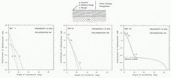
Fig. 6. Theoretical behaviour of σ° with incidence angle at 13 GHz and HH polarization. The ice surface has constant values of σ = 0.37 cm and l = 8.5 cm. and the three plots a. b. and с represent the back-scatter responses for smooth (σ = 0.15 cm. l = 8.5 cm). medium rough (σ = 0.37 cm. l = 8.5 cm), and rough (σ = 0.81cm, l = 8.2 cm) snow surfaces, respectively.
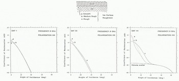
Fig. 7. Theoretical behaviour of σ° with incidence angle at 9 GHz and HH polarization for a snow surface of roughness a - 0.5 cm and l = 5.0 cm. Plots for day 1. day 22, and day 44 indicate the response to three grades of ice-surface roughness corresponding to the rough, medium rough, and rough surfaces described in Figure 6.
4.2. Model Indications
Figures 6 and 7 display the predicted behaviour of σ° with incidence angle, each at three different stages in the period of observations, and at 13 and 9 GHz, respectively. Figure 6 shows that snow-surface roughness changes influence surface scattering only during the early stages of snow-cover development. After 22 d, the effect of varying snow-surface statistics has little effect on the modelled back-scattering. This phenomenon can be explained by the fact that despite high transmissivities at the surface, the penetration depth is minimal owing to the brine content of the snow cover. Back-scatter is high at angles close to normal incidence, and back-scatter fall-off with angle is rapid. Thus, despite increasing dry-snow permittivities due to densification, it appears that the angular back-scatter signature is controlled primarily by the brine content. As the snow cover evolves, the brine content decreases and, despite increases in snow density, the contribution from snow-surface scatter is reduced. At this later stage of snow-cover development, the effects of surface roughness become negligible, as the reduced brine-volume fractions allow incident energy to penetrate as far as the frazil-ice surface beneath.
A very different situation can be seen in Figure 7. Because of extinction and absorption in the snow layer during the first 1Od (when wicking of brine strongly influences permittivities), the ice-surface roughness has a negligible effect on the angular variation in the back-scatter coefficient. However, beyond day 10, our analyses suggest that the effects of brine volume are sufficiently reduced for small variations in the scatter signatures to be observed. Contributions from ice-surface scatter are, nonetheless, only observed between 0° and 20°. For incidence angles greater than about 30°, we calculate that the effects of surface scattering from beneath such a snow layer of 0.03 m or more in depth are negligible. This applies to ice-surface roughness normally encountered on young ice, since most of the energy directed towards the interface at the transmission angle is reflected away from the instrument.
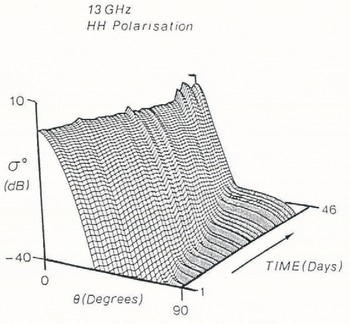
Fig. 8. Trend surface in three-dimensional space illustrating changes of σ with time over the range 0–90° of incidence angles at a frequency of 13GHz.
The upper snow-surface scattering term dominates in the early period (1–10 d), because of the high brine-volume fractions and increased extinction in the snow layer. The angular response of σ° is very narrow and typically falls by 50 dB in the first 20° away from the normal. For rougher surfaces σ does, however, demonstrate lower gradients, but at typical synthetic aperture radar (SAR) or side-looking airborne radar (SLAR) incidence angles of between 30° and 70°, σ° is negligible at C-, X-, and Ku-bands for the first 20 d.
It is not until after 25 d have passed that the volumetric scatter contribution from the snow layer becomes significant (see Figs 6 and 7). The continuing densification and concurrent brine-volume reduction up to day 46 lead to higher volume back-scatter values. Extinction coefficients are minimized and scattering by the snow volume contributes to maximum observed values for ![]() of around −20 dB by day 46.
of around −20 dB by day 46.
The three-dimensional trend surfaces in Figures 8 and 9 describe the predicted transitions occurring in the back-scatter signatures over the 46 d period, for Ku- and C-band (for HH polarization). For 13 GHz (Fig. 8), the overall trend is toward a small increase in σ° at normal incidence, and a fairly stable angular fall-off between 10° and 30°, which is composed entirely of surface scatter from the two dielectric interfaces. In contrast, σ° is seen to increase almost linearly with time in the angular interval 35–90°. Small daily events observed in the original sampled data are also seen to contribute to day-to-day fluctuations, manifested as small undulations in the three-dimensional plot.
In the lower-frequency X- and C-bands, reductions in the magnitude of both the small-scale fluctuations and the long-term increases over 46 d can be seen. At X-band, the volume-scattering contribution does not feature as prominently as at higher frequencies, attaining maximum predicted values of the order of 10 dB lower than at Ku-band by the end of the 46 d period. Increasing the wavelength to 5.66 cm (C-band) leads to the situation where the contrast in scattering conditions over the total observation period is negligible. Figure 9 illustrates this trend with σ° displayed as almost the same linear function of θ throughout the 46 d. Importantly, the volume-scattering contribution remains below –40 dB, since the scattering efficiency of the snow crystals is reduced the longer the wavelength.
Finally, we highlight the respective contributions of both surface and volume scattering for snow surfaces of differing degrees of roughness, at selected stages of the 46 d period. Figure 10 illustrates that a reversal occurs in this 3 cm brine-wetted snow layer, whereupon volume scatter increases above surface scatter. This reversal shifts in frequency as the physical and dielectric properties of the snow layer evolve.
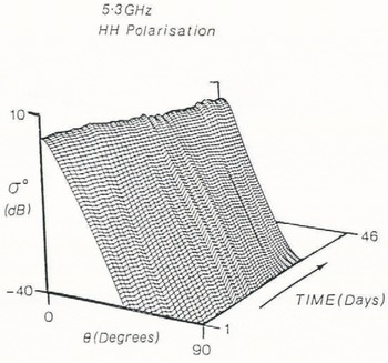
Fig. 9. Trend surface in three-dimensional space illustrating changes of a with time over the range 0—90° of incidence angles at a frequency of 5.3 GHz.
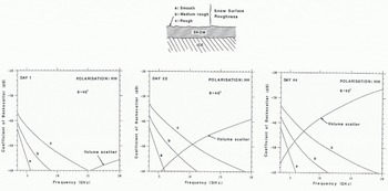
Fig. 10. Relative contributions of surface and volume scatter for the evolving snow Iayter for days 1.22, and 44 over the GHz frequency range. Snow-surface roughness varies while ice-surface roughness remains constant at σ = 0.37 cm, l = 8.5 cm.
5. Conclusions
We have observed a number of important changes in the physical and electromagnetic properties of a snow cover on cold, young sea ice which lead to significant variations in the surface-scattering properties. The modelled back-scatter and dielectric properties are first approximations based on the conditions found in Resolute Passage during the winter of 1982, and cannot be assumed to be representative of all young, snow-covered sea ice. Although the results of Delker and others (1980Reference Delker, Onstott and Moorea, Reference Delker, Onstott and Mooreb) are available for comparison, the ice temperature and salinity conditions at their site, which are critical to scattering, were not exactly the same. We cannot, therefore, draw direct comparisons between our results and their measured back-scatter values.
Small-scale roughness plays an important role in determining the back-scatter coefficient during the early stages of ice and snow-cover development in Resolute Passage, and detailed statistics must evidently be obtained for the roughness of snow-covered young ice forms before more accurate absolute values of σ° can be predicted. Recently, Reference Onstott, Kim and MooreOnstott and others (1983) measured standard deviations of surface heights and surface-correlation lengths on snow-free summer and fall ice surfaces, and found that calculated correlation functions displayed exponential decay. However, since no statistics are available for cold snow-covered thin ice surfaces, there is no a priori justification for using a Gaussian or exponential correlation function in the scattering model at this stage. As even with an exponential correlation function, surface roughness may account for as much as 15 dB difference in σ° at large incidence angles (Kim, unpublished), this is an important problem and one that will only be resolved with the collection of more detailed surface-roughness information. Our models suggest that small variations may also be caused by brine-volume, temperature, and density variations, but not the bulk properties of the ice, which remained nearly constant during the study period.
These findings have a number of implications for the interpretation of SAR and SLAR imagery, particularly where it is necessary to distinguish young ice forms from either open water or thicker first-year ice. The results show that further work on the seasonal variations in the physical and dielectric properties of snow-covered sea ice and their effects on the back-scatter from the surface is required before ice types can be identified, without ambiguity, from radar imagery.
Acknowledgements
M.R.D. acknowledges support from a U.K. Natural Environment Research Council studentship. The field part of the project was funded by the Arctic Institute of North America, the Department of Indian and Northern Affairs (Canada), and the Natural Sciences and Engineering Research Council of Canada. Logistical support was provided by the Polar Continental Shelf Project, and field assistance was provided by A.T. Roberts. We also wish to thank F. Carsey, J.G. Paren, and J. Bamber for helpful discussions and suggestions during this work.


