


1 Introduction and main results
Let $G = \langle S \rangle $
denote the rank-r free group with generating set
$G = \langle S \rangle $
denote the rank-r free group with generating set $S = \{s_{1}, \ldots , s_{r}\}$
and identity e, and let
$S = \{s_{1}, \ldots , s_{r}\}$
and identity e, and let $(X,\mu ,T)$
be a measure-preserving G-system, that is, T is a homomorphism from G to the automorphism group of the standard probability space
$(X,\mu ,T)$
be a measure-preserving G-system, that is, T is a homomorphism from G to the automorphism group of the standard probability space $(X,\mu )$
. We will not need to make explicit use of the
$(X,\mu )$
. We will not need to make explicit use of the $\sigma $
-algebra on X, so we leave it unnamed.
$\sigma $
-algebra on X, so we leave it unnamed.
An observable on X is a measurable map with domain X. In this paper the codomain will be a finite set endowed with the discrete sigma algebra; in this case we call the map a finite observable and the codomain an alphabet.
Any observable $\alpha {\colon}\! X \to \mathtt {A}$
induces a map
$\alpha {\colon}\! X \to \mathtt {A}$
induces a map $\alpha ^{G} {\colon}\! X \to \mathtt {A}^{G}$
by setting
$\alpha ^{G} {\colon}\! X \to \mathtt {A}^{G}$
by setting
 $$ \begin{align*} (\alpha^{G}(x))_{g} = \alpha(T_{g} x) \quad \text{for all } g \in G. \end{align*} $$
We call the $\mathtt {A}$
-coloring
$\mathtt {A}$
-coloring $\alpha ^{G}(x)$
of G the itinerary of x, since it records the observations that will be made over the entire orbit of x under the action of G. We also similarly define the map
$\alpha ^{G}(x)$
of G the itinerary of x, since it records the observations that will be made over the entire orbit of x under the action of G. We also similarly define the map $\alpha ^{H} {\colon}\! X \to \mathtt {A}^{H}$
for any subset H of G. We abbreviate
$\alpha ^{H} {\colon}\! X \to \mathtt {A}^{H}$
for any subset H of G. We abbreviate $\alpha ^{n} := \alpha ^{\mathrm {B}(e,n)}$
, where
$\alpha ^{n} := \alpha ^{\mathrm {B}(e,n)}$
, where $\mathrm {B}(e,n)$
is the closed ball of radius n centered at the identity in G, which is endowed with the word-length metric. If
$\mathrm {B}(e,n)$
is the closed ball of radius n centered at the identity in G, which is endowed with the word-length metric. If $\beta {\colon}\! X \to \mathtt {B}$
is a second finite observable, we denote by
$\beta {\colon}\! X \to \mathtt {B}$
is a second finite observable, we denote by $\alpha \beta {\colon}\! X \to \mathtt {A} \times \mathtt {B}$
the map
$\alpha \beta {\colon}\! X \to \mathtt {A} \times \mathtt {B}$
the map $\alpha \beta (x) = (\alpha (x), \beta (x))$
.
$\alpha \beta (x) = (\alpha (x), \beta (x))$
.
The (Shannon) entropy of a finite observable $\alpha {\colon}\! X \to \mathtt {A}$
is defined by
$\alpha {\colon}\! X \to \mathtt {A}$
is defined by
 $$ \begin{align*} \mathrm{H}_{\mu} (\alpha) = - \sum_{a \in \mathtt{A}} \alpha_{*}\mu (a) \log \alpha_{*} \mu(a) , \end{align*} $$
where $\alpha _{*} \mu \in \operatorname {\mathrm {Prob}}(\mathtt {A})$
is the pushforward measure, with the convention
$\alpha _{*} \mu \in \operatorname {\mathrm {Prob}}(\mathtt {A})$
is the pushforward measure, with the convention $0 \log 0 = 0$
. The entropy of
$0 \log 0 = 0$
. The entropy of $\alpha $
can be interpreted as the expected amount of information revealed by observing
$\alpha $
can be interpreted as the expected amount of information revealed by observing $\alpha $
, assuming its distribution
$\alpha $
, assuming its distribution $\alpha _{*} \mu $
is known.
$\alpha _{*} \mu $
is known.
An early application of Shannon’s entropy to ergodic theory was its use by Kolmogorov and Sinai to show that there exist non-isomorphic Bernoulli shifts over $\mathbb {Z}$
. A Bernoulli shift over
$\mathbb {Z}$
. A Bernoulli shift over $\mathbb {Z}$
is a system of the form
$\mathbb {Z}$
is a system of the form $(\mathtt {A}^{\mathbb {Z}}, \mu ^{\mathbb {Z}}, S)$
for some alphabet
$(\mathtt {A}^{\mathbb {Z}}, \mu ^{\mathbb {Z}}, S)$
for some alphabet $\mathtt {A}$
and
$\mathtt {A}$
and $\mu \in \operatorname {\mathrm {Prob}}(\mathtt {A})$
; S is the shift action of
$\mu \in \operatorname {\mathrm {Prob}}(\mathtt {A})$
; S is the shift action of $\mathbb {Z}$
. They did this by defining an entropy rate for
$\mathbb {Z}$
. They did this by defining an entropy rate for $\mathbb {Z}$
-systems, which can be interpreted as the average information per unit time revealed by observing the system. For a Bernoulli shift
$\mathbb {Z}$
-systems, which can be interpreted as the average information per unit time revealed by observing the system. For a Bernoulli shift $(\mathtt {A}^{\mathbb {Z}}, \mu ^{\mathbb {Z}}, S)$
, the entropy rate is simply the ‘base entropy’
$(\mathtt {A}^{\mathbb {Z}}, \mu ^{\mathbb {Z}}, S)$
, the entropy rate is simply the ‘base entropy’ $\mathrm {H}_{\mu }(\alpha )$
, where
$\mathrm {H}_{\mu }(\alpha )$
, where $\alpha {\colon}\! \mathtt {A}^{n} \to \mathtt {A}$
is the ‘time zero’ observable.
$\alpha {\colon}\! \mathtt {A}^{n} \to \mathtt {A}$
is the ‘time zero’ observable.
Isomorphism invariance of the Kolmogorov–Sinai entropy rate is typically proven using the fact that entropy rate is non-increasing under factor maps (which are surjective homomorphisms of measure-preserving systems). This fact can be interpreted as stating that a system cannot simulate another system that is ‘more random’.
The entropy rate was soon generalized to systems acted on by an arbitrary amenable group (such as $\mathbb {Z}^{d}$
). Extending beyond amenable groups proved more difficult, and in fact it was found to be impossible for such an extension to preserve all desirable properties of the Kolmogorov–Sinai entropy rate. In particular, an entropy rate for non-amenable group actions which assigns Bernoulli shifts their base entropy cannot be non-increasing under factor maps [Reference Ornstein and Weiss13, Appendix C].
$\mathbb {Z}^{d}$
). Extending beyond amenable groups proved more difficult, and in fact it was found to be impossible for such an extension to preserve all desirable properties of the Kolmogorov–Sinai entropy rate. In particular, an entropy rate for non-amenable group actions which assigns Bernoulli shifts their base entropy cannot be non-increasing under factor maps [Reference Ornstein and Weiss13, Appendix C].
The first invariant to distinguish between Bernoulli shifts over free groups is Lewis Bowen’s f-invariant. Following [Reference Bowen2], this can be defined by
 $$ \begin{align*} F_{\mu} (T, \alpha) &= (1-2r) \mathrm{H}_{\mu} (\alpha) + \sum_{i=1}^{r} \mathrm{H}_{\mu} (\alpha^{\{e,s_{i}\}}), \\ f_{\mu} (T, \alpha) &= \inf_{n} F_{\mu} (T, \alpha^{n}) = \lim_{n \to \infty} F_{\mu} (T, \alpha^{n}). \end{align*} $$
The main theorem of [Reference Bowen3] is that $f_{\mu }(T, \alpha )$
depends on the observable
$f_{\mu }(T, \alpha )$
depends on the observable $\alpha $
only through the
$\alpha $
only through the $\sigma $
-algebra it generates. In particular, the common value of
$\sigma $
-algebra it generates. In particular, the common value of $f_{\mu } (T, \alpha )$
among all
$f_{\mu } (T, \alpha )$
among all $\alpha $
which generate the
$\alpha $
which generate the $\sigma $
-algebra of the measurable space X (assuming such
$\sigma $
-algebra of the measurable space X (assuming such $\alpha $
exist) is a measure-conjugacy invariant of the system
$\alpha $
exist) is a measure-conjugacy invariant of the system $(X, \mu , T)$
. In the same paper, Bowen showed that the f-invariant of a Bernoulli shift is the Shannon entropy of the base measure; in particular, Bernoulli shifts with different base entropies are non-isomorphic.
$(X, \mu , T)$
. In the same paper, Bowen showed that the f-invariant of a Bernoulli shift is the Shannon entropy of the base measure; in particular, Bernoulli shifts with different base entropies are non-isomorphic.
In [Reference Bowen2], Bowen gave an alternate formula for the f-invariant, which we now introduce.
For any homomorphism $\sigma {\colon}\! G \to \operatorname {\mathrm {Sym}}(n)$
we have a G-system
$\sigma {\colon}\! G \to \operatorname {\mathrm {Sym}}(n)$
we have a G-system $([n], \operatorname {\mathrm {Unif}}(n), \sigma )$
, and we can consider a labeling
$([n], \operatorname {\mathrm {Unif}}(n), \sigma )$
, and we can consider a labeling $\mathbf {x} \in \mathtt {A}^{n}$
as an
$\mathbf {x} \in \mathtt {A}^{n}$
as an $\mathtt {A}$
-valued observable on this system. We denote the law of its itinerary by
$\mathtt {A}$
-valued observable on this system. We denote the law of its itinerary by $P^{\sigma }_{\mathbf {x}} = \mathbf {x}^{G}_{*}\operatorname {\mathrm {Unif}}(n)$
and call this the empirical distribution of
$P^{\sigma }_{\mathbf {x}} = \mathbf {x}^{G}_{*}\operatorname {\mathrm {Unif}}(n)$
and call this the empirical distribution of $\mathbf {x}$
. We say that
$\mathbf {x}$
. We say that $\mathbf {x}$
is a good model for
$\mathbf {x}$
is a good model for $\alpha $
over
$\alpha $
over $\sigma $
if it is difficult to distinguish the G-systems
$\sigma $
if it is difficult to distinguish the G-systems $(X,\mu , T)$
and
$(X,\mu , T)$
and $([n], \operatorname {\mathrm {Unif}}(n), \sigma )$
via their respective observables
$([n], \operatorname {\mathrm {Unif}}(n), \sigma )$
via their respective observables $\alpha $
and
$\alpha $
and $\mathbf {x}$
. To make this precise, we denote
$\mathbf {x}$
. To make this precise, we denote
 $$ \begin{align*} \Omega(\sigma, \mathcal{O}) := \{ \mathbf{x} \in \mathtt{A}^{n} : P^{\sigma}_{\mathbf{x}} \in \mathcal{O} \}, \end{align*} $$
which is a set of good models for $\alpha $
over
$\alpha $
over $\sigma $
if
$\sigma $
if $\mathcal {O}$
is a weak
$\mathcal {O}$
is a weak $^{*}$
-open neighborhood of
$^{*}$
-open neighborhood of $\alpha ^{G}_{*}\mu \in \operatorname {\mathrm {Prob}}(\mathtt {A}^{G})$
; the particular set
$\alpha ^{G}_{*}\mu \in \operatorname {\mathrm {Prob}}(\mathtt {A}^{G})$
; the particular set $\mathcal {O}$
quantifies how good the models are. The alphabet
$\mathcal {O}$
quantifies how good the models are. The alphabet $\mathtt {A}$
is given the discrete topology and
$\mathtt {A}$
is given the discrete topology and $\mathtt {A}^{G}$
the product topology, so ‘weak
$\mathtt {A}^{G}$
the product topology, so ‘weak $^{*}$
-close’ means marginals on some finite sets are close in total variation norm.
$^{*}$
-close’ means marginals on some finite sets are close in total variation norm.
For each $n \in \mathbb {N}$
, let
$n \in \mathbb {N}$
, let $\mathtt {s}_{n} = \operatorname {\mathrm {Unif}}(\operatorname {\mathrm {Hom}}(G, \operatorname {\mathrm {Sym}}(n)))$
. Bowen showed in [Reference Bowen2] that the f-invariant is given by
$\mathtt {s}_{n} = \operatorname {\mathrm {Unif}}(\operatorname {\mathrm {Hom}}(G, \operatorname {\mathrm {Sym}}(n)))$
. Bowen showed in [Reference Bowen2] that the f-invariant is given by
 $$ \begin{align*} f_{\mu} (T, \alpha) = \inf_{\mathcal{O} \ni \alpha^{G}_{*}\mu} \limsup_{n \to \infty} \frac{1}{n} \log \mathop{\mathbb{E}}\limits_{\sigma \sim \mathtt{s}_{n}} \lvert \Omega(\sigma, \mathcal{O}) \rvert. \end{align*} $$
To make an analogy with statistical physics, we can think of $\alpha ^{G}_{*} \mu $
as a macroscopic statistical distribution of the state of a system; then the f-invariant is the exponential growth rate of the expected number of ‘microstates’ that are consistent with these statistics. What we here call good models are often called microstates for this reason.
$\alpha ^{G}_{*} \mu $
as a macroscopic statistical distribution of the state of a system; then the f-invariant is the exponential growth rate of the expected number of ‘microstates’ that are consistent with these statistics. What we here call good models are often called microstates for this reason.
More generally, given any random or deterministic sofic approximation $\Sigma = \{\mathtt {s}_{n}\}_{n=1}^{\infty }$
, we can define the sofic entropy relative to
$\Sigma = \{\mathtt {s}_{n}\}_{n=1}^{\infty }$
, we can define the sofic entropy relative to $\Sigma $
by
$\Sigma $
by
 $$ \begin{align*} \mathrm{h}_{\Sigma,\mu} (T, \alpha) = \inf_{\mathcal{O} \ni \alpha^{G}_{*}\mu} \limsup_{n \to \infty} \frac{1}{n} \log \mathop{\mathbb{E}}\limits_{\sigma \sim \mathtt{s}_{n}} \lvert \Omega(\sigma, \mathcal{O}) \rvert. \end{align*} $$
Here each $\mathtt {s}_{n}$
is a probability measure on the set of functions
$\mathtt {s}_{n}$
is a probability measure on the set of functions $G \to \operatorname {\mathrm {Sym}}(n)$
which is supported on functions which are approximately free homomorphisms.
$G \to \operatorname {\mathrm {Sym}}(n)$
which is supported on functions which are approximately free homomorphisms.
This paper is motivated by a desire to better understand the dependence of sofic entropy on the sofic approximation $\Sigma $
. For any choice of
$\Sigma $
. For any choice of $\Sigma $
, the sofic entropy agrees with Kolmogorov–Sinai entropy if the acting group is amenable [Reference Bowen6] and with the Shannon entropy of the base if the system is a Bernoulli shift [Reference Bowen4]. For some systems, the sofic entropy can be finite relative to some sofic approximations and
$\Sigma $
, the sofic entropy agrees with Kolmogorov–Sinai entropy if the acting group is amenable [Reference Bowen6] and with the Shannon entropy of the base if the system is a Bernoulli shift [Reference Bowen4]. For some systems, the sofic entropy can be finite relative to some sofic approximations and $-\infty $
relative to others. It is unknown whether two deterministic sofic approximations can yield different finite entropy values for the same system.
$-\infty $
relative to others. It is unknown whether two deterministic sofic approximations can yield different finite entropy values for the same system.
In this paper, we express the entropy relative to a type of stochastic block model in terms of the relative f-invariant, which we now introduce.
If $\alpha ,\beta $
are two finite observables with codomains
$\alpha ,\beta $
are two finite observables with codomains $\mathtt {A},\mathtt {B}$
, the conditional entropy is
$\mathtt {A},\mathtt {B}$
, the conditional entropy is
 $$ \begin{align*} \mathrm{H}_{\mu} (\alpha | \beta) = \mathrm{H}_{\mu} (\alpha \beta) - \mathrm{H}_{\mu} (\beta). \end{align*} $$
This can be interpreted as the expected amount of information revealed by observing $\alpha $
if both the value of
$\alpha $
if both the value of $\beta $
and the joint distribution of
$\beta $
and the joint distribution of $\alpha $
and
$\alpha $
and $\beta $
are known. The relative f-invariant is defined by
$\beta $
are known. The relative f-invariant is defined by
 $$ \begin{align*} F_{\mu}(T, \alpha | \beta) &= F_{\mu} (T, \alpha \beta) - F_{\mu} (T, \beta) \\ &= (1-2r) \mathrm{H}_{\mu} (\alpha|\beta) + \sum_{i=1}^{r} \mathrm{H}_{\mu} (\alpha^{\{e,s_{i}\}} \mid \beta^{\{e,s_{i}\}}), \\ f_{\mu} (T, \alpha | \beta) &= \inf_{k_{1} \in \mathbb{N}} \sup_{k_{2} \in \mathbb{N}} F_{\mu} (T, \alpha^{k_{1}} \mid \beta^{k_{2}}). \end{align*} $$
Both the infimum and supremum can be replaced by limits; this follows from Lemma 3.2 below. It follows from Corollary 3.5 that we could also directly define
 $$ \begin{align*} f_{\mu} (T, \alpha | \beta) = f_{\mu}(T, \alpha {} \beta) - f_{\mu}(T, \beta) , \end{align*} $$
as long as $f_{\mu }(T, \beta )> -\infty $
.
$f_{\mu }(T, \beta )> -\infty $
.
We now define the relevant type of stochastic block model. If H is a finite subset of G, we denote by $d^{H}(\mu , \nu )$
the total variation distance between the marginals of
$d^{H}(\mu , \nu )$
the total variation distance between the marginals of $\mu $
and
$\mu $
and $\nu $
on
$\nu $
on $\mathtt {A}^{H}$
. Our convention for the total variation distance between measures
$\mathtt {A}^{H}$
. Our convention for the total variation distance between measures $\mu , \nu \in \operatorname {\mathrm {Prob}}(\mathtt {A})$
is
$\mu , \nu \in \operatorname {\mathrm {Prob}}(\mathtt {A})$
is
 $$ \begin{align*} \| \mu - \nu \|_{\operatorname{\mathrm{TV}}} = \frac{1}{2} \sum_{a \in \mathtt{A}} \lvert \mu\{a\} - \nu\{a\} \rvert. \end{align*} $$
For each $k \in \mathbb {N}$
we define a pseudometric on
$k \in \mathbb {N}$
we define a pseudometric on $\operatorname {\mathrm {Prob}}(\mathtt {A}^{G})$
by
$\operatorname {\mathrm {Prob}}(\mathtt {A}^{G})$
by
 $$ \begin{align*} d^{*}_{k}(\mu, \nu) = \sum_{i \in [r]} d^{\mathrm{B}(e,k) \cup \mathrm{B}(s_{i},k)}(\mu, \nu). \end{align*} $$
Note that $\{d_{k}^{*}\}_{k \in \mathbb {N}}$
together generate the weak
$\{d_{k}^{*}\}_{k \in \mathbb {N}}$
together generate the weak $^{*}$
topology on
$^{*}$
topology on $\operatorname {\mathrm {Prob}}(\mathtt {A}^{G})$
. These generalize the function
$\operatorname {\mathrm {Prob}}(\mathtt {A}^{G})$
. These generalize the function $d_{\sigma }^{*}$
from [Reference Bowen2], which corresponds to the case
$d_{\sigma }^{*}$
from [Reference Bowen2], which corresponds to the case $k=0$
. For
$k=0$
. For $\mathcal {O} = \{\nu \in \operatorname {\mathrm {Prob}}(\mathtt {A}^{G}) : d^{*}_{k}(\alpha ^{G}_{*} \mu , \nu ) < \varepsilon \}$
we write
$\mathcal {O} = \{\nu \in \operatorname {\mathrm {Prob}}(\mathtt {A}^{G}) : d^{*}_{k}(\alpha ^{G}_{*} \mu , \nu ) < \varepsilon \}$
we write
 $$ \begin{align*} \Omega(\sigma, \mathcal{O}) =: \Omega^{*}_{k}(\sigma, \alpha, \varepsilon) \subseteq \mathtt{A}^{n}. \end{align*} $$
Our stochastic block model is now defined as follows: given $\mathbf {y}_{0} \in \mathtt {B}^{n}$
,
$\mathbf {y}_{0} \in \mathtt {B}^{n}$
, $\sigma _{0} \in \operatorname {\mathrm {Hom}}(G, \operatorname {\mathrm {Sym}}(n))$
, and
$\sigma _{0} \in \operatorname {\mathrm {Hom}}(G, \operatorname {\mathrm {Sym}}(n))$
, and $k \in \mathbb {N}$
, let
$k \in \mathbb {N}$
, let
 $$ \begin{align*} \mathtt{SBM}(\sigma_{0}, \mathbf{y}_{0}, k) := \operatorname{\mathrm{Unif}}(\{ \sigma \in \operatorname{\mathrm{Hom}}(G, \operatorname{\mathrm{Sym}}(n)) : d^{*}_{k}(P_{\mathbf{y}_{0}}^{\sigma}, P_{\mathbf{y}_{0}}^{\sigma_{0}}) = 0 \}). \end{align*} $$
The labeling $\mathbf {y}_{0}$
partitions the elements of
$\mathbf {y}_{0}$
partitions the elements of $[n]$
into
$[n]$
into $\lvert \mathtt {B} \rvert $
communities, and we can think of the random homomorphism
$\lvert \mathtt {B} \rvert $
communities, and we can think of the random homomorphism $\sigma $
as a random choice of directed edges between and within the communities. Certain statistics of these random edge choices are determined by the reference homomorphism
$\sigma $
as a random choice of directed edges between and within the communities. Certain statistics of these random edge choices are determined by the reference homomorphism $\sigma _{0}$
; note that for
$\sigma _{0}$
; note that for $k>0$
these statistics are more precise than those specified by a standard stochastic block model. In §2 we define weights, which are the objects used to record the relevant statistics.
$k>0$
these statistics are more precise than those specified by a standard stochastic block model. In §2 we define weights, which are the objects used to record the relevant statistics.
1.1 Main results
Our main theorems show that the relative f-invariant can be interpreted as the growth rate of the expected number of ways to extend a planted good model for $\beta $
to a good model for
$\beta $
to a good model for $\alpha \beta $
, over a stochastic block model which has statistics determined by
$\alpha \beta $
, over a stochastic block model which has statistics determined by $\beta $
and its planted model.
$\beta $
and its planted model.
We first prove that if $\beta ^{G}_{*}\mu $
is Markov then we can use a stochastic block model which only takes into account ‘one-step statistics’.
$\beta ^{G}_{*}\mu $
is Markov then we can use a stochastic block model which only takes into account ‘one-step statistics’.
Theorem A. Let $\alpha {\colon}\! X \to \mathtt {A}$
and
$\alpha {\colon}\! X \to \mathtt {A}$
and $\beta {\colon}\! X \to \mathtt {B}$
be finite observables, and for each n let
$\beta {\colon}\! X \to \mathtt {B}$
be finite observables, and for each n let $\mathbf {y}_{n} \in \mathtt {B}^{n}$
and
$\mathbf {y}_{n} \in \mathtt {B}^{n}$
and $\sigma _{n} \in \operatorname {\mathrm {Hom}}(G, \operatorname {\mathrm {Sym}}(n))$
be such that
$\sigma _{n} \in \operatorname {\mathrm {Hom}}(G, \operatorname {\mathrm {Sym}}(n))$
be such that
 $$ \begin{align*} \lim_{n \to \infty} d_{0}^{*}(P_{\mathbf{y}_{n}}^{\sigma_{n}}, \beta^{G}_{*}\mu) = 0. \end{align*} $$
Suppose that $\beta ^{G}_{*} \mu $
is a Markov measure. With
$\beta ^{G}_{*} \mu $
is a Markov measure. With $\mathtt {s}_{n} = \mathtt {SBM}(\sigma _{n},\mathbf {y}_{n}, 0)$
, we have
$\mathtt {s}_{n} = \mathtt {SBM}(\sigma _{n},\mathbf {y}_{n}, 0)$
, we have
 $$ \begin{align*} f_{\mu}(T,\alpha \mid \beta) = \inf_{\mathcal{O} \ni (\alpha\beta)^{G}_{*} \mu} \limsup_{n \to \infty} \frac{1}{n} \log \mathop{\mathbb{E}}\limits_{\sigma \sim \mathtt{s}_{n}} \lvert \{ \mathbf{x} \in \mathtt{A}^{n} : (\mathbf{x},\mathbf{y}_{n}) \in \Omega(\sigma, \mathcal{O}) \} \rvert. \end{align*} $$
Proposition A. The assumptions of Theorem A are non-vacuous; that is, for any finite observable $\beta {\colon}\! X \to \mathtt {B}$
there exist sequences
$\beta {\colon}\! X \to \mathtt {B}$
there exist sequences $\{\mathbf {y}_{n} \in \mathtt {B}^{n}\}_{n=1}^{\infty }$
and
$\{\mathbf {y}_{n} \in \mathtt {B}^{n}\}_{n=1}^{\infty }$
and $\{ \sigma _{n} \in \operatorname {\mathrm {Hom}}(G, \operatorname {\mathrm {Sym}}(n)) \}_{n=1}^{\infty }$
such that
$\{ \sigma _{n} \in \operatorname {\mathrm {Hom}}(G, \operatorname {\mathrm {Sym}}(n)) \}_{n=1}^{\infty }$
such that $\lim _{n \to \infty } d_{0}^{*}(P_{\mathbf {y}_{n}}^{\sigma _{n}}, \beta ^{G}_{*}\mu ) = 0$
.
$\lim _{n \to \infty } d_{0}^{*}(P_{\mathbf {y}_{n}}^{\sigma _{n}}, \beta ^{G}_{*}\mu ) = 0$
.
This follows from the fact that free group actions are ‘sofic’, which is proven for example in [Reference Dykema, Kerr and Pichot10, Reference Păunescu14, Reference Popa15]. A more elementary proof is given in §4 below.
If $\beta ^{G}_{*} \mu $
is not Markov, then the same formula holds with a more precise type of stochastic block model.
$\beta ^{G}_{*} \mu $
is not Markov, then the same formula holds with a more precise type of stochastic block model.
Theorem B. Let $\alpha {\colon}\! X \to \mathtt {A}$
and
$\alpha {\colon}\! X \to \mathtt {A}$
and $\beta {\colon}\! X \to \mathtt {B}$
be finite observables. Let
$\beta {\colon}\! X \to \mathtt {B}$
be finite observables. Let $m_{n}$
approach infinity as n goes to infinity while satisfying
$m_{n}$
approach infinity as n goes to infinity while satisfying $m_{n} = o(\log \log n)$
. For each n, let
$m_{n} = o(\log \log n)$
. For each n, let $\mathbf {y}_{n} \in \mathtt {B}^{n}$
and
$\mathbf {y}_{n} \in \mathtt {B}^{n}$
and $\sigma _{n} \in \operatorname {\mathrm {Hom}}(G, \operatorname {\mathrm {Sym}}(n))$
be such that
$\sigma _{n} \in \operatorname {\mathrm {Hom}}(G, \operatorname {\mathrm {Sym}}(n))$
be such that
 $$ \begin{align*} d_{m_{n}}^{*}(P_{\mathbf{y}_{n}}^{\sigma_{n}}, \beta^{G}_{*}\mu) = O \bigg( \frac{1}{\log n} \bigg). \end{align*} $$
Suppose that $f_{\mu }(T, \beta )> -\infty $
. With
$f_{\mu }(T, \beta )> -\infty $
. With $\mathtt {s}_{n} = \mathtt {SBM}(\sigma _{n}, \mathbf {y}_{n}, m_{n})$
,
$\mathtt {s}_{n} = \mathtt {SBM}(\sigma _{n}, \mathbf {y}_{n}, m_{n})$
,
 $$ \begin{align*} f_{\mu} (T, \alpha \mid \beta) = \inf_{\mathcal{O} \ni (\alpha\beta)^{G}_{*}\mu} \limsup_{n \to \infty} \frac{1}{n} \log \mathop{\mathbb{E}}\limits_{\sigma \sim \mathtt{s}_{n}} \lvert \{ \mathbf{x} \in \mathtt{A}^{n} : (\mathbf{x}, \mathbf{y}_{n}) \in \Omega(\sigma, \mathcal{O}) \} \rvert. \end{align*} $$
Proposition B. The assumptions of Theorem B are non-vacuous; that is, for any finite observable $\beta {\colon}\! X \to \mathtt {B}$
and any sequence
$\beta {\colon}\! X \to \mathtt {B}$
and any sequence $\{m_{n} \in \mathbb {N}\}_{n=1}^{\infty }$
approaching infinity while satisfying
$\{m_{n} \in \mathbb {N}\}_{n=1}^{\infty }$
approaching infinity while satisfying $m_{n} = o(\log \log n)$
, there exist sequences
$m_{n} = o(\log \log n)$
, there exist sequences $\{\mathbf {y}_{n} \in \mathtt {B}^{n}\}_{n=1}^{\infty }$
and
$\{\mathbf {y}_{n} \in \mathtt {B}^{n}\}_{n=1}^{\infty }$
and $\{ \sigma _{n} \in \operatorname {\mathrm {Hom}}(G, \operatorname {\mathrm {Sym}}(n)) \}_{n=1}^{\infty }$
such that
$\{ \sigma _{n} \in \operatorname {\mathrm {Hom}}(G, \operatorname {\mathrm {Sym}}(n)) \}_{n=1}^{\infty }$
such that $\lim _{n \to \infty } d_{m_{n}}^{*}(P_{\mathbf {y}_{n}}^{\sigma _{n}}, \beta ^{G}_{*}\mu ) = O ( {1}/{\log n} )$
.
$\lim _{n \to \infty } d_{m_{n}}^{*}(P_{\mathbf {y}_{n}}^{\sigma _{n}}, \beta ^{G}_{*}\mu ) = O ( {1}/{\log n} )$
.
Using Theorem B, we prove the following formula for the growth rate of the expected number of good models over a stochastic block model. This can be compared to the variational principle in [Reference Kerr and Li12], and has a similar proof.
Theorem C. Let $\mathtt {s}_{n}, \alpha , \beta $
be as in the statement of Theorem B. Then
$\mathtt {s}_{n}, \alpha , \beta $
be as in the statement of Theorem B. Then
 $$ \begin{align*} \inf_{\mathcal{O} \ni \alpha^{G}_{*}\mu} \limsup_{n \to \infty} \frac{1}{n} \log \mathop{\mathbb{E}}\limits_{\sigma \sim \mathtt{s}_{n}} \lvert \Omega(\sigma, \mathcal{O}) \rvert = \sup_{\lambda \in \mathsf{J}(\alpha_{*}^{G} \mu,\, \beta_{*}^{G} \mu)} f_{\lambda} (S, \mathtt{a} \mid \mathtt{b}). \end{align*} $$
Here $\mathsf {J}(\alpha _{*}^{G} \mu ,\, \beta _{*}^{G} \mu )$
is the set of joinings of the G-systems
$\mathsf {J}(\alpha _{*}^{G} \mu ,\, \beta _{*}^{G} \mu )$
is the set of joinings of the G-systems $(\mathtt {A}^{G}, \alpha ^{G}_{*}\mu , S)$
and
$(\mathtt {A}^{G}, \alpha ^{G}_{*}\mu , S)$
and $(\mathtt {B}^{G}, \beta ^{G}_{*}\mu , S)$
, that is, shift-invariant probability measures on
$(\mathtt {B}^{G}, \beta ^{G}_{*}\mu , S)$
, that is, shift-invariant probability measures on $(\mathtt {A} \times \mathtt {B})^{G}$
whose
$(\mathtt {A} \times \mathtt {B})^{G}$
whose $\mathtt {A}^{G}, \mathtt {B}^{G}$
marginals are
$\mathtt {A}^{G}, \mathtt {B}^{G}$
marginals are $\alpha _{*}^{G} \mu ,\, \beta _{*}^{G} \mu $
, respectively. S denotes the shift action of G. We use
$\alpha _{*}^{G} \mu ,\, \beta _{*}^{G} \mu $
, respectively. S denotes the shift action of G. We use $\mathtt {a}, \mathtt {b}$
to denote the maps
$\mathtt {a}, \mathtt {b}$
to denote the maps
 $$ \begin{align*} \mathtt{a} {\colon} (\mathtt{A}\times \mathtt{B})^{G} &\to \mathtt{A} \\ ( (a_{g},b_{g}) )_{g \in G} &\mapsto a_{e} \end{align*} $$
and
 $$ \begin{align*} \mathtt{b} {\colon} (\mathtt{A} \times \mathtt{B})^{G} &\to \mathtt{B} \\ ( (a_{g},b_{g}) )_{g \in G} &\mapsto b_{e}, \end{align*} $$
which observe the $\mathtt {A}$
(respectively,
$\mathtt {A}$
(respectively, $\mathtt {B}$
) label at the identity.
$\mathtt {B}$
) label at the identity.
Note that the supremum is always greater than or equal to $f_{\mu } (T, \alpha )$
, with equality attained by the product joining; this means that the expected number of good models for
$f_{\mu } (T, \alpha )$
, with equality attained by the product joining; this means that the expected number of good models for $\alpha $
over a block model with built-in good models for any
$\alpha $
over a block model with built-in good models for any $\beta $
is at least the expected number of good models over a uniformly random homomorphism. It is possible for the supremum to be strictly larger, however. For example, suppose
$\beta $
is at least the expected number of good models over a uniformly random homomorphism. It is possible for the supremum to be strictly larger, however. For example, suppose $f_{\mu } (T, \alpha ) < 0$
and
$f_{\mu } (T, \alpha ) < 0$
and $\alpha = \beta $
, and let
$\alpha = \beta $
, and let $\lambda $
be the diagonal joining. Then
$\lambda $
be the diagonal joining. Then
 $$ \begin{align*} f_{\lambda}(S, \mathtt{a} \mid \mathtt{b}) = 0> f_{\mu} (T, \alpha). \end{align*} $$
1.2 Related work
The expressions appearing on the right-hand sides of Theorems A and B are very closely related to Ben Hayes’ definition of ‘relative sofic entropy in the presence’ [Reference Hayes11, Definition 2.5]. Some differences are that we consider expected numbers of good models over random sofic approximations, and that Hayes takes a supremum inside the logarithm over which good model is to be extended, while we fix a sequence $\{\mathbf {y}_{n}\}$
of planted good models. Hayes also does not restrict to shift systems as we do here.
$\{\mathbf {y}_{n}\}$
of planted good models. Hayes also does not restrict to shift systems as we do here.
In [Reference Coja-Oghlan, Hahn-Klimroth, Loick, Müller, Panagiotou, Pasch, Bläser and Monmege8], the free energy (that is, the limit of normalized log partition functions) over a type of stochastic block model is shown to satisfy a variational principle; see Propositions 3.6 and 3.7 of that paper.
1.3 Random sofic approximations
As noted above, the f-invariant is closely related to another invariant of measure-preserving systems called sofic entropy, which was introduced by Bowen in [Reference Bowen4].
A homomorphism $\sigma \in \operatorname {\mathrm {Hom}}(G, \operatorname {\mathrm {Sym}}(n))$
is called
$\sigma \in \operatorname {\mathrm {Hom}}(G, \operatorname {\mathrm {Sym}}(n))$
is called $(D,\delta )$
-sofic for some finite
$(D,\delta )$
-sofic for some finite $D \subset G$
and
$D \subset G$
and $\delta> 0$
if
$\delta> 0$
if
 $$ \begin{align*} \lvert \{ j \in [n] : \sigma(\gamma) j \neq j \text{ for all } \gamma \in D \setminus\{e\} \} \rvert> (1-\delta) n. \end{align*} $$
A sequence of homomorphisms $\Sigma = (\sigma _{n} \in \operatorname {\mathrm {Hom}}(G, \operatorname {\mathrm {Sym}}(n)) )_{n \in \mathbb {N}}$
is called a sofic approximation if, for every
$\Sigma = (\sigma _{n} \in \operatorname {\mathrm {Hom}}(G, \operatorname {\mathrm {Sym}}(n)) )_{n \in \mathbb {N}}$
is called a sofic approximation if, for every $(D,\delta )$
, the homomorphism
$(D,\delta )$
, the homomorphism $\sigma _{n}$
is
$\sigma _{n}$
is $(D,\delta )$
-sofic for all large enough n.
$(D,\delta )$
-sofic for all large enough n.
The sofic entropy relative to $\Sigma $
is the exponential growth rate of the number of good models over
$\Sigma $
is the exponential growth rate of the number of good models over $\sigma _{n}$
. Specifically, for any finite observable
$\sigma _{n}$
. Specifically, for any finite observable $\alpha $
on X we have
$\alpha $
on X we have
 $$ \begin{align*} \mathrm{h}_{\Sigma,\mu}(T, \alpha) = \inf_{\mathcal{O} \ni \alpha_{*}^{G} \mu} \limsup_{n \to \infty} \frac{1}{n} \log \lvert \Omega (\sigma_{n}, \mathcal{O}) \rvert. \end{align*} $$
This is an isomorphism invariant of the system $(X, \mu , T)$
if
$(X, \mu , T)$
if $\alpha $
is any generating observable, that is if the
$\alpha $
is any generating observable, that is if the $\sigma $
-algebra of the measurable space X is the coarsest one which is shift-invariant and
$\sigma $
-algebra of the measurable space X is the coarsest one which is shift-invariant and $\alpha $
-measurable.
$\alpha $
-measurable.
By analogy with this expression, we might call the sequences of random homomorphisms appearing in expressions above ‘random sofic approximations’. The following proposition provides further justification for this terminology.
Proposition 1.1. If $(\mathtt {s}_{n})$
is any of the sequences appearing in Theorems A, B, and C, then for any
$(\mathtt {s}_{n})$
is any of the sequences appearing in Theorems A, B, and C, then for any $(D,\delta )$
there exists
$(D,\delta )$
there exists $\varepsilon>0$
such that
$\varepsilon>0$
such that
 $$ \begin{align*} \mathop{\mathbb{P}}\limits_{\sigma \sim \mathtt{s}_{n}} ( \sigma \text{ is } (D,\delta) \text{-sofic} ) \geq 1 - n^{-\varepsilon n} \end{align*} $$
for all large enough n.
In particular, if $\sigma _{1} \sim \mathtt {s}_{1}$
,
$\sigma _{1} \sim \mathtt {s}_{1}$
, $\sigma _{2} \sim \mathtt {s}_{2}$
etc. are independent then
$\sigma _{2} \sim \mathtt {s}_{2}$
etc. are independent then $(\sigma _{n})$
is a sofic approximation with probability 1.
$(\sigma _{n})$
is a sofic approximation with probability 1.
1.4 Organization
In §2 we define weights and discuss some of their useful properties. In §3 we prove a few basic results about the functions f and F. Some of the results of these two sections are used in §4 to show that the assumptions of the main theorems are not vacuous. In §5 we show how the function F is related to the number of homomorphism-labeling pairs $(\sigma , \mathbf {y})$
that realize a given weight, which is the main ingredient of the proofs of Theorems A and B given in the next two sections. In §8 we show how to deduce Theorem C from Theorem B. Section 9 contains a proof of Proposition 1.1. The final section contains a proof of Lemma 2.3, which asserts that a weight can be approximated by a denominator-n weight with a specified marginal.
$(\sigma , \mathbf {y})$
that realize a given weight, which is the main ingredient of the proofs of Theorems A and B given in the next two sections. In §8 we show how to deduce Theorem C from Theorem B. Section 9 contains a proof of Proposition 1.1. The final section contains a proof of Lemma 2.3, which asserts that a weight can be approximated by a denominator-n weight with a specified marginal.
2 Weights
If $\alpha {\colon}\! X \to \mathtt {A}$
is a finite observable, for
$\alpha {\colon}\! X \to \mathtt {A}$
is a finite observable, for $a,a^{\prime } \in \mathtt {A}$
and
$a,a^{\prime } \in \mathtt {A}$
and $i \in [r]$
let
$i \in [r]$
let
 $$ \begin{align*} W_{\alpha}(a,a^{\prime}; i) = \alpha_{*}^{\{e,s_{i}\}} \mu(a,a^{\prime}) = \mu\{ x \in X : \alpha(x) = a,\ \alpha(T_{s_{i}} x) = a^{\prime}\} \end{align*} $$
and also denote
 $$ \begin{align*} W_{\alpha}(a) = \alpha_{*}\mu(a). \end{align*} $$
For $\mathbf {x} \in \mathtt {A}^{n}$
and
$\mathbf {x} \in \mathtt {A}^{n}$
and $\sigma \in \operatorname {\mathrm {Hom}}(G, \operatorname {\mathrm {Sym}}(n))$
let
$\sigma \in \operatorname {\mathrm {Hom}}(G, \operatorname {\mathrm {Sym}}(n))$
let
 $$ \begin{align*} W_{\sigma, \mathbf{x}}(a,a^{\prime}; i) = P^{\sigma, \{e,s_{i}\}}_{\mathbf{x}} (a,a^{\prime}) \end{align*} $$
and $W_{\sigma , \mathbf {x}}(a) = P^{\sigma , \{e\}}_{\mathbf {x}} (a)$
. This could equivalently be defined as a special case of the previous construction, with
$W_{\sigma , \mathbf {x}}(a) = P^{\sigma , \{e\}}_{\mathbf {x}} (a)$
. This could equivalently be defined as a special case of the previous construction, with $\sigma $
specifying an action on
$\sigma $
specifying an action on $X = [n]$
with an observable
$X = [n]$
with an observable $\mathbf {x} {\colon}\! [n] \to \mathtt {A}$
.
$\mathbf {x} {\colon}\! [n] \to \mathtt {A}$
.
More abstractly, any $W \in ( \operatorname {\mathrm {Prob}}(\mathtt {A}^{2}) )^{r}$
is called an
$W \in ( \operatorname {\mathrm {Prob}}(\mathtt {A}^{2}) )^{r}$
is called an $\mathtt {A}$
-weight if
$\mathtt {A}$
-weight if
 $$ \begin{align*} \sum_{a^{\prime} \in \mathtt{A}} W(a, a^{\prime}; i) = \sum_{a^{\prime} \in \mathtt{A}} W(a^{\prime}, a; j) \end{align*} $$
for all $i,j \in [r]$
and
$i,j \in [r]$
and $a \in \mathtt {A}$
. For each
$a \in \mathtt {A}$
. For each $a \in \mathtt {A}$
we denote this common value by
$a \in \mathtt {A}$
we denote this common value by $W(a)$
. Note that the objects
$W(a)$
. Note that the objects $W_{\alpha }$
and
$W_{\alpha }$
and $W_{\sigma , \mathbf {x}}$
defined above satisfy this condition.
$W_{\sigma , \mathbf {x}}$
defined above satisfy this condition.
We say that W has denominator n if $n \cdot W(a,a^{\prime };i) \in \mathbb {N}$
for all
$n \cdot W(a,a^{\prime };i) \in \mathbb {N}$
for all $a,a^{\prime },i$
.
$a,a^{\prime },i$
.
The measures $W(\cdot ,\cdot; i)$
for
$W(\cdot ,\cdot; i)$
for $i \in [r]$
are called the edge measures of W, and
$i \in [r]$
are called the edge measures of W, and $W(\cdot )$
is called the vertex measure.
$W(\cdot )$
is called the vertex measure.
For any alphabet $\mathtt {A}$
, we use the metric on
$\mathtt {A}$
, we use the metric on $\mathtt {A}$
-weights defined by
$\mathtt {A}$
-weights defined by
 $$ \begin{align*} d(W_{1}, W_{2}) &:= \sum_{i \in [r]} \| { W_{1}(\cdot, \cdot; i) - W_{2}(\cdot, \cdot; i)}\|_{\operatorname{\mathrm{TV}}} \\ &= \frac{1}{2} \sum_{i \in [r]} \sum_{a,a^{\prime} \in \mathtt{A}} \lvert W_{1}(a,a^{\prime}; i) - W_{2}(a,a^{\prime}; i) \rvert. \end{align*} $$
We can use weights to count good models up to equivalence under the pseudometrics $d^{*}_{k}$
using the following proposition.
$d^{*}_{k}$
using the following proposition.
Proposition 2.1. If $\sigma \in \operatorname {\mathrm {Hom}}(G, \operatorname {\mathrm {Sym}}(n))$
and
$\sigma \in \operatorname {\mathrm {Hom}}(G, \operatorname {\mathrm {Sym}}(n))$
and $\mathbf {x} \in \mathtt {A}^{n}$
, then for any observable
$\mathbf {x} \in \mathtt {A}^{n}$
, then for any observable $\alpha {\colon}\! X \to ~\mathtt {A}$
,
$\alpha {\colon}\! X \to ~\mathtt {A}$
,
 $$ \begin{align*} d(W_{\sigma, \mathbf{x}^{k}}, W_{\alpha^{k}}) = d^{*}_{k}(P_{\mathbf{x}}^{\sigma}, \alpha^{G}_{*} \mu). \end{align*} $$
Note this implies also that
 $$ \begin{align*} d^{*}_{k}(P_{\mathbf{x}}^{\sigma}, \alpha^{G}_{*} \mu) = d^{*}_{0}(P_{\mathbf{x}^{k}}^{\sigma}, (\alpha^{k})^{G}_{*} \mu). \end{align*} $$
Proof. By definition of the distance between weights,
 $$ \begin{align*} d(W_{\sigma, \mathbf{x}^{k}}, W_{\alpha^{k}}) &= \frac{1}{2} \sum_{i \in [r]} \sum_{\mathbf{a}, \mathbf{a}^{\prime} \in \mathtt{A}^{\mathrm{B}(e,k)}} \lvert W_{\sigma, \mathbf{x}^{k}}( \mathbf{a}, \mathbf{a}^{\prime}; i) - W_{\alpha^{k}}(\mathbf{a}, \mathbf{a}^{\prime}; i) \rvert \\ &= \frac{1}{2} \sum_{i \in [r]} \sum_{\mathbf{a}, \mathbf{a}^{\prime} \in \mathtt{A}^{\mathrm{B}(e,k)}} \bigg\lvert\, \frac{1}{n} \bigg\lvert \left\{ j \in [n] : \begin{array}{@{}c@{}} (\mathbf{x}^{k})_{j} = \mathbf{a} \\ (\mathbf{x}^{k})_{\sigma(s_{i})j} = \mathbf{a}^{\prime} \end{array}\right\} \bigg\rvert \\ &\quad - \mu \left\{ x \in X : \begin{array}{@{}c@{}} \alpha^{k}(x) = \mathbf{a} \\ \alpha^{k}(T_{s_{i}}x) = \mathbf{a}^{\prime} \end{array}\right\} \bigg\rvert. \end{align*} $$
For many ‘incompatible’ pairs $\mathbf {a},\mathbf {a}^{\prime }$
, both terms will be zero: suppose
$\mathbf {a},\mathbf {a}^{\prime }$
, both terms will be zero: suppose $g \in \mathrm {B}(e,k) \cap \mathrm {B}(s_{i},k)$
, so that
$g \in \mathrm {B}(e,k) \cap \mathrm {B}(s_{i},k)$
, so that $g s_{i}^{-1} \in \mathrm {B}(e,k)$
. If the second term in the absolute value is non-zero, then for some
$g s_{i}^{-1} \in \mathrm {B}(e,k)$
. If the second term in the absolute value is non-zero, then for some $x \in X$
we have
$x \in X$
we have $\alpha ^{k}(x) = \mathbf {a}$
and
$\alpha ^{k}(x) = \mathbf {a}$
and $\alpha ^{k}(T_{s_{i}}x) = \mathbf {a}^{\prime }$
, and therefore
$\alpha ^{k}(T_{s_{i}}x) = \mathbf {a}^{\prime }$
, and therefore
 $$ \begin{align*} \mathbf{a}^{\prime}_{g s_{i}^{-1}} = (\alpha^{k}(T_{s_{i}}x))_{g s_{i}^{-1}} = \alpha(T_{g s_{i}^{-1}} T_{s_{i}} x) = \alpha(T_{g} x) = (\alpha^{k} (x) )_{g} = \mathbf{a}_{g}. \end{align*} $$
The same argument shows that $\mathbf {a}^{\prime }_{g s_{i}^{-1}} = \mathbf {a}_{g}$
for all
$\mathbf {a}^{\prime }_{g s_{i}^{-1}} = \mathbf {a}_{g}$
for all $g \in \mathrm {B}(e,k) \cap \mathrm {B}(s_{i},k)$
whenever the first term is non-zero. Therefore we can restrict the sum to pairs
$g \in \mathrm {B}(e,k) \cap \mathrm {B}(s_{i},k)$
whenever the first term is non-zero. Therefore we can restrict the sum to pairs $\mathbf {a}, \mathbf {a}^{\prime }$
with
$\mathbf {a}, \mathbf {a}^{\prime }$
with $\mathbf {a}^{\prime }_{g s_{i}^{-1}} = \mathbf {a}_{g}$
for all
$\mathbf {a}^{\prime }_{g s_{i}^{-1}} = \mathbf {a}_{g}$
for all $g \in \mathrm {B}(e,k) \cap \mathrm {B}(s_{i},k)$
. Equivalently, we can sum over all
$g \in \mathrm {B}(e,k) \cap \mathrm {B}(s_{i},k)$
. Equivalently, we can sum over all $\mathbf {A} \in \mathtt {A}^{\mathrm {B}(e,k) \cup \mathrm {B}(s_{i},k)}$
to get
$\mathbf {A} \in \mathtt {A}^{\mathrm {B}(e,k) \cup \mathrm {B}(s_{i},k)}$
to get
 $$ \begin{align*} d(W_{\sigma, \mathbf{x}^{k}}, W_{\alpha^{k}}) &= \frac{1}{2} \sum_{i \in [r]} \sum_{\mathbf{A} \in \mathtt{A}^{\mathrm{B}(e,k) \cup \mathrm{B}(s_{i},k)}} \bigg\lvert \frac{1}{n} \lvert \{ j \in [n] : ( \mathbf{x}^{\mathrm{B}(e,k) \cup \mathrm{B}(s_{i},k)} )_{j} = \mathbf{A} \} \rvert \\ &\quad - \mu \{ x \in X : \alpha^{\mathrm{B}(e,k) \cup \mathrm{B}(s_{i},k)} (x) = \mathbf{A} \} \bigg\rvert \\ &= \sum_{i \in [r]} d^{\mathrm{B}(e,k) \cup \mathrm{B}(s_{i},k)} ( P_{\mathbf{x}}^{\sigma}, \alpha_{*}^{G} \mu).\\[-3.5pc] \end{align*} $$
It will be useful to consider the pushforward map induced by a map between alphabets: if $\pi {\colon}\! \mathtt {A} \to \mathtt {B}$
is a measurable map and W is an
$\pi {\colon}\! \mathtt {A} \to \mathtt {B}$
is a measurable map and W is an $\mathtt {A}$
-weight, then
$\mathtt {A}$
-weight, then $\pi W$
is the
$\pi W$
is the $\mathtt {B}$
-weight given by
$\mathtt {B}$
-weight given by
 $$ \begin{align*} \pi W(b, b^{\prime}; i) = \sum_{a \in \pi^{-1}\{b\}} \sum_{a^{\prime} \in \pi^{-1}\{b^{\prime}\}} W(a,a^{\prime}; i). \end{align*} $$
Note that this implies that the vertex measure of W is
 $$ \begin{align*} \pi W(b) = \sum_{a \in \pi^{-1}\{b\}} W(a). \end{align*} $$
For example, let $\pi _{\mathtt {B}} {\colon}\! \mathtt {A} \times \mathtt {B} \to \mathtt {B}$
be the projection map. If W is an
$\pi _{\mathtt {B}} {\colon}\! \mathtt {A} \times \mathtt {B} \to \mathtt {B}$
be the projection map. If W is an $\mathtt {A} \times \mathtt {B}$
-weight then
$\mathtt {A} \times \mathtt {B}$
-weight then $\pi _{\mathtt {B}} W$
is given by
$\pi _{\mathtt {B}} W$
is given by
 $$ \begin{align*} \pi_{\mathtt{B}} W(b_{1}) = \sum_{a \in \mathtt{A}} W((a,b_{1})) \quad \pi_{\mathtt{B}} W(b_{1}, b_{2}; i) = \sum_{a_{1}, a_{2} \in \mathtt{A}} W ((a_{1}, b_{1}), (a_{2}, b_{2}); i ). \end{align*} $$
We call this the $\mathtt {B}$
-marginal of W.
$\mathtt {B}$
-marginal of W.
All weights in the present paper will be over alphabets of the form $\mathtt {A}^{\mathrm {B}(e,k)} \times \mathtt {B}^{\mathrm {B}(e,k^{\prime })}$
. We use this fact to introduce some simplified notation for projections.
$\mathtt {A}^{\mathrm {B}(e,k)} \times \mathtt {B}^{\mathrm {B}(e,k^{\prime })}$
. We use this fact to introduce some simplified notation for projections.
-
• $\pi _{A}$
denotes projection onto the entire
$\mathtt {A}$
factor
$\mathtt {A}^{\mathrm {B}(e,k)}$
;
$\pi _{B}$
is used similarly.
$\pi _{A}$
denotes projection onto the entire
$\mathtt {A}$
factor
$\mathtt {A}^{\mathrm {B}(e,k)}$
;
$\pi _{B}$
is used similarly. -
• For
$m<k$
and
$m^{\prime }<k^{\prime }$
,
$\pi _{m,m^{\prime }}$
denotes projection onto
$\mathtt {A}^{\mathrm {B}(e,m)} \times \mathtt {B}^{\mathrm {B}(e,m^{\prime })}$
. -
•
$\pi _{m}$
denotes the projection
$\mathtt {A}^{\mathrm {B}(e,k)} \to \mathtt {A}^{\mathrm {B}(e,m)}$
, except that if
$m=0$
we write
$\pi _{e}$
.


We define $F(W)$
for an abstract weight W by
$F(W)$
for an abstract weight W by
 $$ \begin{align*} F(W) = (1-2r) \mathrm{H} ( W(\cdot) ) + \sum_{i \in [r]} \mathrm{H} ( W(\cdot, \cdot; i) ) \end{align*} $$
where H is the Shannon entropy. Note that this is consistent with the above definitions in that, for example,
 $$ \begin{align*} F(W_{\alpha}) = F_{\mu} (T, \alpha). \end{align*} $$
We can revisit the definition of our version of the stochastic block model using weights. Let $H \subset G$
and let W be a denominator-
$H \subset G$
and let W be a denominator- $n\ \mathtt {B}^{\mathrm {B}(e,k)}$
-weight. Suppose there exist
$n\ \mathtt {B}^{\mathrm {B}(e,k)}$
-weight. Suppose there exist $\mathbf {y} \in \mathtt {B}^{n}$
and
$\mathbf {y} \in \mathtt {B}^{n}$
and $\sigma \in \operatorname {\mathrm {Hom}}(G, \operatorname {\mathrm {Sym}}(n))$
such that
$\sigma \in \operatorname {\mathrm {Hom}}(G, \operatorname {\mathrm {Sym}}(n))$
such that $W = W_{\sigma , \mathbf {y}^{k}}$
. Then
$W = W_{\sigma , \mathbf {y}^{k}}$
. Then
 $$ \begin{align*} \mathtt{SBM}(\sigma, \mathbf{y}, k) = \operatorname{\mathrm{Unif}}(\{ \sigma^{\prime} \in \operatorname{\mathrm{Hom}}(G, \operatorname{\mathrm{Sym}}(n)) : W_{\sigma^{\prime}, \mathbf{y}^{k}} = W \}) , \end{align*} $$
so we can also denote this distribution by $\mathtt {SBM}(\mathbf {y}, W)$
. Specifying the distribution by a weight rather than a specific homomorphism will occasionally be more convenient.
$\mathtt {SBM}(\mathbf {y}, W)$
. Specifying the distribution by a weight rather than a specific homomorphism will occasionally be more convenient.
2.1 Constructing weights and good models
We borrow the first result of this type from [Reference Bowen2]; it allows us to find a denominator-n approximation to a given weight.
Lemma 2.2. (Lemma 2.3 of [Reference Bowen2])
There is a constant C such that for any $\mathtt {A}$
-weight W there is a denominator-
$\mathtt {A}$
-weight W there is a denominator- $n\ \mathtt {A}$
-weight within distance
$n\ \mathtt {A}$
-weight within distance $C \lvert \mathtt {A} \rvert ^{2} r/n$
of W.
$C \lvert \mathtt {A} \rvert ^{2} r/n$
of W.
The following lemma allows us not only to construct a denominator-n approximation to a given weight, but also to specify a marginal of this approximation:
Lemma 2.3. Let W be an $\mathtt {A} \times \mathtt {B}$
-weight. If
$\mathtt {A} \times \mathtt {B}$
-weight. If $W_{\mathtt {B}}$
is a
$W_{\mathtt {B}}$
is a $\mathtt {B}$
-weight of denominator n with
$\mathtt {B}$
-weight of denominator n with $d(W_{\mathtt {B}}, \pi _{\mathtt {B}} W) < \delta $
then there is an
$d(W_{\mathtt {B}}, \pi _{\mathtt {B}} W) < \delta $
then there is an $\mathtt {A} \times \mathtt {B}$
-weight
$\mathtt {A} \times \mathtt {B}$
-weight $W_{\mathtt {A}\mathtt {B}}$
with denominator n such that
$W_{\mathtt {A}\mathtt {B}}$
with denominator n such that $\pi _{\mathtt {B}} W_{\mathtt {A}\mathtt {B}} = W_{\mathtt {B}}$
and
$\pi _{\mathtt {B}} W_{\mathtt {A}\mathtt {B}} = W_{\mathtt {B}}$
and $d(W_{\mathtt {A}\mathtt {B}}, W) < 265r ( \lvert \mathtt {A} \times \mathtt {B} \rvert ^{2} / n + \delta )$
.
$d(W_{\mathtt {A}\mathtt {B}}, W) < 265r ( \lvert \mathtt {A} \times \mathtt {B} \rvert ^{2} / n + \delta )$
.
The construction is fairly involved, so it is postponed to §10. The constant 265 is not intended to be optimal.
The definition of a weight $W_{\sigma , \mathbf {x}^{k}}$
in terms of a homomorphism
$W_{\sigma , \mathbf {x}^{k}}$
in terms of a homomorphism $\sigma $
and a labeling
$\sigma $
and a labeling $\mathbf {x}$
is straightforward. However, we will also need to know whether a given weight can be realized in this way. The next two results address this inverse problem.
$\mathbf {x}$
is straightforward. However, we will also need to know whether a given weight can be realized in this way. The next two results address this inverse problem.
Proposition 2.4. If W is a denominator- $n\ \mathtt {A}$
-weight, then there exist
$n\ \mathtt {A}$
-weight, then there exist $\mathbf {x} \in \mathtt {A}^{n}$
and
$\mathbf {x} \in \mathtt {A}^{n}$
and $\sigma \in \operatorname {\mathrm {Hom}}(G, \operatorname {\mathrm {Sym}}(n))$
such that
$\sigma \in \operatorname {\mathrm {Hom}}(G, \operatorname {\mathrm {Sym}}(n))$
such that $W = W_{\sigma , \mathbf {x}}$
.
$W = W_{\sigma , \mathbf {x}}$
.
Proof. This is implied by Proposition 2.1 of [Reference Bowen2].
Unfortunately, this does not imply that for every denominator- $n\ \mathtt {A}^{\mathrm {B}(e,k)}$
-weight W there is some
$n\ \mathtt {A}^{\mathrm {B}(e,k)}$
-weight W there is some $\sigma \in \operatorname {\mathrm {Hom}}(G, \operatorname {\mathrm {Sym}}(n))$
and
$\sigma \in \operatorname {\mathrm {Hom}}(G, \operatorname {\mathrm {Sym}}(n))$
and $\mathbf {x} \in \mathtt {A}^{n}$
such that
$\mathbf {x} \in \mathtt {A}^{n}$
such that $W = W_{\sigma , \mathbf {x}^{k}}$
; instead it provides
$W = W_{\sigma , \mathbf {x}^{k}}$
; instead it provides $\mathbf {X} \in (\mathtt {A}^{\mathrm {B}(e,k)})^{n}$
such that
$\mathbf {X} \in (\mathtt {A}^{\mathrm {B}(e,k)})^{n}$
such that $W = W_{\sigma , \mathbf {X}}$
.
$W = W_{\sigma , \mathbf {X}}$
.
However, if we already know that W is close to a weight of the form $W_{\alpha ^{k}}$
for some observable
$W_{\alpha ^{k}}$
for some observable $\alpha $
, then the following proposition shows that W is also close to a weight of the form
$\alpha $
, then the following proposition shows that W is also close to a weight of the form $W_{\sigma , \mathbf {x}^{k}}$
.
$W_{\sigma , \mathbf {x}^{k}}$
.
Proposition 2.5. Let $\alpha {\colon}\! X \to \mathtt {A}$
,
$\alpha {\colon}\! X \to \mathtt {A}$
, $\sigma \in \operatorname {\mathrm {Hom}}(G, \operatorname {\mathrm {Sym}}(n))$
, and
$\sigma \in \operatorname {\mathrm {Hom}}(G, \operatorname {\mathrm {Sym}}(n))$
, and $\mathbf {X} \in (\mathtt {A}^{\mathrm {B}(e,k)})^{n}$
be such that
$\mathbf {X} \in (\mathtt {A}^{\mathrm {B}(e,k)})^{n}$
be such that $d(W_{\sigma , \mathbf {X}}, W_{\alpha ^{k}}) \leq \varepsilon $
for some
$d(W_{\sigma , \mathbf {X}}, W_{\alpha ^{k}}) \leq \varepsilon $
for some $\varepsilon \geq 0$
. Writing
$\varepsilon \geq 0$
. Writing $\mathbf {x} = \pi _{e} \mathbf {X} \in \mathtt {A}^{n}$
, we have
$\mathbf {x} = \pi _{e} \mathbf {X} \in \mathtt {A}^{n}$
, we have
 $$ \begin{align*} d(W_{\sigma, \mathbf{X}}, W_{\sigma, \mathbf{x}^{k}}) \leq 2r \lvert \mathrm{B}(e,k) \rvert \varepsilon. \end{align*} $$
An immediate consequence is that $\mathbf {X} \in \Omega _{0}^{*}(\sigma , \alpha ^{k}, \varepsilon )$
implies
$\mathbf {X} \in \Omega _{0}^{*}(\sigma , \alpha ^{k}, \varepsilon )$
implies $\pi _{e} \mathbf {X} \in \Omega _{k}^{*}(\sigma , \alpha , c \varepsilon )$
where
$\pi _{e} \mathbf {X} \in \Omega _{k}^{*}(\sigma , \alpha , c \varepsilon )$
where $c = 1 + 2r \lvert \mathrm {B}(e,k) \rvert $
; cf. Claim 2 in the proof of Proposition 3.2 of [Reference Bowen2].
$c = 1 + 2r \lvert \mathrm {B}(e,k) \rvert $
; cf. Claim 2 in the proof of Proposition 3.2 of [Reference Bowen2].
Proof. Claim 4 in the proof of Proposition 3.2 of [Reference Bowen2] implies that
 $$ \begin{align*} \lvert \{ j \in [n] : \mathbf{X}(j) \ne \mathbf{x}^{k}(j) \} \rvert \leq n \lvert \mathrm{B}(e,k) \rvert \varepsilon. \end{align*} $$
It follows that for any $i \in [r]$
,
$i \in [r]$
,
 $$ \begin{align*} &\hspace{-2em} \lvert \{ j \in [n] : \mathbf{X}^{\{e, s_{i}\}}(j) \ne (\mathbf{x}^{k})^{\{e,s_{i}\}}(j) \} \rvert \\[4pt] &\leq \lvert \{ j \in [n] : \mathbf{X}(j) \ne \mathbf{x}^{k}(j) \} \rvert + \lvert \{ j \in [n] : \mathbf{X}(\sigma(s_{i})j) \ne \mathbf{x}^{k}(\sigma(s_{i})j) \} \rvert \\[4pt] &\leq 2 n \lvert \mathrm{B}(e,k) \rvert \varepsilon , \end{align*} $$
so
 $$ \begin{align*} d(W_{\sigma, \mathbf{X}}, W_{\sigma, \mathbf{x}^{k}}) &= \sum_{i \in [r]} \|{ (\mathbf{X}^{\{e, s_{i}\}})_{*} \operatorname{\mathrm{Unif}}(n) - ((\mathbf{x}^{k})^{\{e, s_{i}\}})_{*} \operatorname{\mathrm{Unif}}(n)}\|_{\operatorname{\mathrm{TV}}} \\[4pt] &\leq \sum_{i \in [r]} 2 \lvert \mathrm{B}(e,k) \rvert \varepsilon = 2 r \lvert \mathrm{B}(e,k) \rvert \varepsilon.\\[-3.5pc] \end{align*} $$
The following corollary of the first part of the proof will be useful later. It says that if the weight $W_{\sigma , \mathbf {X}}$
generated by some
$W_{\sigma , \mathbf {X}}$
generated by some $\mathbf {X} \in (\mathtt {A}^{\mathrm {B}(e,k)})^{n}$
and
$\mathbf {X} \in (\mathtt {A}^{\mathrm {B}(e,k)})^{n}$
and $\sigma \in \operatorname {\mathrm {Hom}}(G, \operatorname {\mathrm {Sym}}(n))$
is exactly attainable in some sense, then
$\sigma \in \operatorname {\mathrm {Hom}}(G, \operatorname {\mathrm {Sym}}(n))$
is exactly attainable in some sense, then $\mathbf {X}$
can be exactly recovered from
$\mathbf {X}$
can be exactly recovered from $\sigma $
and the projection
$\sigma $
and the projection $\pi _{e} \mathbf {X} \in ~\mathtt {A}^{n}$
.
$\pi _{e} \mathbf {X} \in ~\mathtt {A}^{n}$
.
Corollary 2.6. Suppose that $\sigma \in \operatorname {\mathrm {Hom}}(G, \operatorname {\mathrm {Sym}}(n))$
and
$\sigma \in \operatorname {\mathrm {Hom}}(G, \operatorname {\mathrm {Sym}}(n))$
and $\mathbf {X} \in (\mathtt {A}^{\mathrm {B}(e,k)})^{n}$
are such that either
$\mathbf {X} \in (\mathtt {A}^{\mathrm {B}(e,k)})^{n}$
are such that either
-
(1)
$W_{\sigma , \mathbf {X}} = W_{\alpha ^{k}}$
for some
$\alpha {\colon}\! X \to \mathtt {A}$
, or -
(2)
$W_{\sigma , \mathbf {X}} = W_{\sigma _{0}, \mathbf {x}_{0}^{k}}$
for some
$\sigma _{0} \in \operatorname {\mathrm {Hom}}(G, \operatorname {\mathrm {Sym}}(m))$
and
$\mathbf {x}_{0} \in \mathtt {A}^{m}$
.


Then $(\pi _{e} \mathbf {X})^{k} = \mathbf {X}$
.
$(\pi _{e} \mathbf {X})^{k} = \mathbf {X}$
.
Note that $(\pi _{e} \mathbf {X})^{k}$
is the k-neighborhood labeling generated from
$(\pi _{e} \mathbf {X})^{k}$
is the k-neighborhood labeling generated from $\pi _{e} \mathbf {X}$
using
$\pi _{e} \mathbf {X}$
using $\sigma $
, rather than
$\sigma $
, rather than $\sigma _{0}$
or some other homomorphism.
$\sigma _{0}$
or some other homomorphism.
Proof. In the first case, we are in the setting of the previous proposition with $\varepsilon =0$
, so the first inequality of its proof gives the claimed result.
$\varepsilon =0$
, so the first inequality of its proof gives the claimed result.
The second case is actually the same; this is only obscured somewhat by the notation. We are in the setting of the previous proposition with the space $X = [m]$
having a G-action specified by
$X = [m]$
having a G-action specified by $\sigma _{0}$
and a finite observable
$\sigma _{0}$
and a finite observable $\mathbf {x}_{0} {\colon}\! [m] \to \mathtt {A}$
.
$\mathbf {x}_{0} {\colon}\! [m] \to \mathtt {A}$
.
3 Properties of F and f
Lemma 3.1. (Continuity as weight function)
If $W_{1}, W_{2}$
are
$W_{1}, W_{2}$
are $\mathtt {A}$
-weights with
$\mathtt {A}$
-weights with $d(W_{1}, W_{2}) \leq \varepsilon \leq 1$
then
$d(W_{1}, W_{2}) \leq \varepsilon \leq 1$
then
 $$ \begin{align*} \lvert F(W_{1}) - F(W_{2}) \rvert \leq 4r ( \mathrm{H}(\varepsilon) + \varepsilon \log_{2} \lvert \mathtt{A} \rvert ) , \end{align*} $$
where $\mathrm {H}(p)$
denotes the entropy of the probability measure
$\mathrm {H}(p)$
denotes the entropy of the probability measure $(p, 1-p) \in \operatorname {\mathrm {Prob}}(\{0,1\})$
.
$(p, 1-p) \in \operatorname {\mathrm {Prob}}(\{0,1\})$
.
Proof. We use Fano’s inequality in the following form (equation (2.139) of [Reference Cover and Thomas9]). Suppose $X,Y$
are
$X,Y$
are $\mathtt {A}$
-valued random variables defined on the same probability space and let
$\mathtt {A}$
-valued random variables defined on the same probability space and let $p_{e} = \mathbb {P}(X \ne Y)$
be their probability of disagreement. Then
$p_{e} = \mathbb {P}(X \ne Y)$
be their probability of disagreement. Then
 $$ \begin{align*} \mathrm{H}(X \mid Y) \leq \mathrm{H}(p_{e}) + p_{e} \log \lvert \mathtt{A} \rvert. \end{align*} $$
Using the chain rule and non-negativity of Shannon entropy, we can deduce that
 $$ \begin{align*} \lvert \mathrm{H}(X) - \mathrm{H}(Y) \rvert \leq \mathrm{H}(p_{e}) + p_{e} \log \lvert \mathtt{A} \rvert. \end{align*} $$
Let $\mu _{1}, \mu _{2} \in \operatorname {\mathrm {Prob}}(\mathtt {A})$
be the respective distributions of
$\mu _{1}, \mu _{2} \in \operatorname {\mathrm {Prob}}(\mathtt {A})$
be the respective distributions of $X_{1},X_{2}$
. Because
$X_{1},X_{2}$
. Because $\| \mu _{1} - \mu _{2} \|_{\operatorname {\mathrm {TV}}}$
is the minimum value of
$\| \mu _{1} - \mu _{2} \|_{\operatorname {\mathrm {TV}}}$
is the minimum value of $\mathbb {P}(X_{1} \ne X_{2})$
over all possible couplings, if
$\mathbb {P}(X_{1} \ne X_{2})$
over all possible couplings, if $\| \mu _{1} - \mu _{2} \|_{\operatorname {\mathrm {TV}}} < \varepsilon $
then
$\| \mu _{1} - \mu _{2} \|_{\operatorname {\mathrm {TV}}} < \varepsilon $
then
 $$ \begin{align*} \lvert \mathrm{H}(\mu_{1}) - \mathrm{H}(\mu_{2}) \rvert \leq \mathrm{H}(\varepsilon) + \varepsilon \log \lvert \mathtt{A} \rvert. \end{align*} $$
The assumed bound $d(W_{1}, W_{2}) \leq \varepsilon $
implies that each vertex and edge measure of
$d(W_{1}, W_{2}) \leq \varepsilon $
implies that each vertex and edge measure of $W_{1}$
is within total variation distance
$W_{1}$
is within total variation distance $\varepsilon $
of its counterpart in
$\varepsilon $
of its counterpart in $W_{2}$
, so
$W_{2}$
, so
 $$ \begin{align*} \lvert F(W_{1}) - F(W_{2}) \rvert &\leq \lvert 1-2r \rvert \cdot \lvert \mathrm{H} ( W_{1}(\cdot) ) - \mathrm{H} ( W_{2}(\cdot) ) \rvert \\ &\quad + \sum_{i \in [r]} \lvert \mathrm{H} ( W_{1}(\cdot, \cdot; i) ) - \mathrm{H} ( W_{2}(\cdot, \cdot; i) ) \rvert \\ &\leq (2r-1) ( \mathrm{H}(\varepsilon) + \varepsilon \log \lvert \mathtt{A} \rvert ) \\ &\quad + r \cdot ( \mathrm{H}(\varepsilon) + \varepsilon \log \lvert \mathtt{A} \rvert^{2} ) \\ &\leq 4r ( \mathrm{H}(\varepsilon) + \varepsilon \log \lvert \mathtt{A} \rvert ).\\[-3.3pc] \end{align*} $$
Let $\alpha {\colon}\! X \to \mathtt {A}$
and
$\alpha {\colon}\! X \to \mathtt {A}$
and $\beta {\colon}\! X \to \mathtt {B}$
be observables. We say that
$\beta {\colon}\! X \to \mathtt {B}$
be observables. We say that $\beta $
is a coarsening of
$\beta $
is a coarsening of $\alpha $
if each part of the partition of X induced by
$\alpha $
if each part of the partition of X induced by $\beta $
is a union of parts of the partition induced by
$\beta $
is a union of parts of the partition induced by $\alpha $
(up to null sets). Equivalently, there is some function
$\alpha $
(up to null sets). Equivalently, there is some function $g {\colon}\! \mathtt {A} \to \mathtt {B}$
such that
$g {\colon}\! \mathtt {A} \to \mathtt {B}$
such that $\beta = g \circ \alpha $
almost surely. In this situation we can also call
$\beta = g \circ \alpha $
almost surely. In this situation we can also call $\alpha $
a refinement of
$\alpha $
a refinement of $\beta $
.
$\beta $
.
A useful property of the Shannon entropy $\mathrm {H}_{\mu }(\alpha )$
is monotonicity under refinement. The function F does not share this property, but it is monotone under the following particular kind of refinement introduced in [Reference Bowen3].
$\mathrm {H}_{\mu }(\alpha )$
is monotonicity under refinement. The function F does not share this property, but it is monotone under the following particular kind of refinement introduced in [Reference Bowen3].
We say that $\beta $
is a simple splitting of
$\beta $
is a simple splitting of $\alpha $
if there is some
$\alpha $
if there is some $s \in \{s_{1}^{\pm 1}, \ldots , s_{r}^{\pm 1}\}$
and a coarsening
$s \in \{s_{1}^{\pm 1}, \ldots , s_{r}^{\pm 1}\}$
and a coarsening $\tilde {\alpha }$
of
$\tilde {\alpha }$
of $\alpha $
such that, up to null sets, the partition induced by
$\alpha $
such that, up to null sets, the partition induced by $\beta $
is the coarsest common refinement of the partitions induced by
$\beta $
is the coarsest common refinement of the partitions induced by $\alpha $
and
$\alpha $
and $\tilde {\alpha } \circ T_{s}$
.
$\tilde {\alpha } \circ T_{s}$
.
We say that $\beta $
is a splitting of
$\beta $
is a splitting of $\alpha $
if there are observables
$\alpha $
if there are observables $\alpha = \beta _{0}, \beta _{1}, \ldots , \beta _{n} = \beta $
such that
$\alpha = \beta _{0}, \beta _{1}, \ldots , \beta _{n} = \beta $
such that $\beta _{i}$
is a simple splitting of
$\beta _{i}$
is a simple splitting of $\beta _{i-1}$
for
$\beta _{i-1}$
for $i = 1, 2, \ldots , n$
. We will use the following monotonicity properties of the relative version of F.
$i = 1, 2, \ldots , n$
. We will use the following monotonicity properties of the relative version of F.
Lemma 3.2. (Monotonicity under splitting)
-
(1) If
$\alpha _{1}$
is a splitting of
$\alpha _{2}$
then
$F(\alpha _{1} | \beta ) \leq F(\alpha _{2} | \beta )$
. -
(2) If
$\beta _{1}$
is a splitting of
$\beta _{2}$
then
$F(\alpha | \beta _{1}) \geq F(\alpha | \beta _{2})$
.


Proof. (1) This is essentially Proposition 5.1 of [Reference Bowen3]; conditioning on $\beta $
makes no difference to the proof.
$\beta $
makes no difference to the proof.
(2) The proof is based on the proof of part (1), but in place of the chain rule for conditional entropy we use the following bound:
 $$ \begin{align*} \mathrm{H}(\alpha \mid \beta_{2}) &\leq \mathrm{H}(\alpha, \beta_{1} \mid \beta_{2})\quad \text{(monotonicity)} \\ &= \mathrm{H}(\beta_{1} \mid \beta_{2}) + \mathrm{H}(\alpha \mid \beta_{1}, \beta_{2}) \quad \text{(chain rule)} \\ &\leq \mathrm{H}(\beta_{1} \mid \beta_{2}) + \mathrm{H}(\alpha \mid \beta_{1}) \quad \text{(monotonicity)}{.} \end{align*} $$
We will also use the following consequence of the previous bound:
 $$ \begin{align*} &\mathrm{H}(\alpha^{\{e,s_{i}\}} \mid \beta_{1}^{\{e,s_{i}\}}) - \mathrm{H}(\alpha^{\{e,s_{i}\}} \mid \beta_{2}^{\{e,s_{i}\}}) \\ &\quad\geq -\mathrm{H}(\beta_{1}^{\{e,s_{i}\}} \mid \beta_{2}^{\{e,s_{i}\}}) \quad \text{(previous bound)} \\ &\quad\geq -( \mathrm{H}(\beta_{1}^{\{s_{i}\}} \mid \beta_{2}^{\{e,s_{i}\}}) + \mathrm{H}(\beta_{1} \mid \beta_{2}^{\{e,s_{i}\}}) ) \quad \text{(subadditivity)} \\ &\quad= -( \mathrm{H}(\beta_{1} \mid \beta_{2}^{\{e,s_{i}^{-1}\}}) + \mathrm{H}(\beta_{1} \mid \beta_{2}^{\{e,s_{i}\}}) ) \quad \text{(}T\text{-invariance of }\mu\text{)}{.} \end{align*} $$
It suffices to check the case where $\beta _{1}$
is a simple splitting of
$\beta _{1}$
is a simple splitting of $\beta _{2}$
. Let
$\beta _{2}$
. Let $t \in \{s_{1}^{\pm 1}, \ldots , s_{r}^{\pm 1} \}$
and let
$t \in \{s_{1}^{\pm 1}, \ldots , s_{r}^{\pm 1} \}$
and let $\tilde {\beta }$
be a coarsening of
$\tilde {\beta }$
be a coarsening of $\beta _{2}$
such that the partition induced by
$\beta _{2}$
such that the partition induced by $\beta _{1}$
is the same as the coarsest common refinement of the partitions induced by
$\beta _{1}$
is the same as the coarsest common refinement of the partitions induced by $\beta _{2}$
and
$\beta _{2}$
and $\tilde {\beta } \circ T_{t}$
up to null sets. Then, using the two bounds just derived,
$\tilde {\beta } \circ T_{t}$
up to null sets. Then, using the two bounds just derived,
 $$ \begin{align*} F(\alpha | \beta_{1}) - F(\alpha | \beta_{2}) &= (1-2r) ( \mathrm{H}(\alpha | \beta_{1}) - \mathrm{H}(\alpha | \beta_{2}) ) \\[4pt] &\quad + \sum_{i \in [r]} ( \mathrm{H}(\alpha^{\{e,s_{i}\}} | \beta_{1}^{\{e,s_{i}\}}) - \mathrm{H}(\alpha^{\{e,s_{i}\}} | \beta_{1}^{\{e,s_{i}\}}) ) \\ &\geq (1-2r) ( - \mathrm{H}(\beta_{1} | \beta_{2}) ) - \sum_{i \in [r]} ( \mathrm{H}(\beta_{1} \mid \beta_{2}^{\{e,s_{i}^{-1}\}})\\ &\quad + \mathrm{H}(\beta_{1} \mid \beta_{2}^{\{e,s_{i}\}}) ) \\ &= (2r-1) \mathrm{H}(\beta_{1} | \beta_{2}) - \sum_{s \in \{s_{1}^{\pm 1} \ldots s_{r}^{\pm 1}\}} \mathrm{H}(\beta_{1} \mid \beta_{2}^{\{e,s\}}) \end{align*} $$
But
 $$ \begin{align*} \mathrm{H}(\beta_{1} \mid \beta_{2}^{\{e,t\}}) \leq \mathrm{H}(\beta_{1} \mid \beta_{2} \tilde{\beta}^{\{t\}}) = 0 , \end{align*} $$
so we can remove the t term from the sum to get
 $$ \begin{align*} F(\alpha | \beta_{1}) - F(\alpha | \beta_{2}) &\geq (2r-1) \mathrm{H}(\beta_{1} | \beta_{2}) - \sum_{s \in \{s_{1}^{\pm 1} \ldots s_{r}^{\pm 1}\} \setminus \{t\}} \mathrm{H}(\beta_{1} \mid \beta_{2}^{\{e,s\}}) \\ &= \sum_{s \in \{s_{1}^{\pm 1} \ldots s_{r}^{\pm 1}\} \setminus \{t\}} ( \mathrm{H}(\beta_{1} | \beta_{2}) - \mathrm{H}(\beta_{1} \mid \beta_{2}^{\{e,s\}}) ) \\ &\geq 0.\\[-3pc] \end{align*} $$
One corollary is the following convenient formula.
Corollary 3.3. Let $\alpha , \beta $
be finite observables such that
$\alpha , \beta $
be finite observables such that $\beta ^{G}_{*}\mu $
is a Markov measure. Then
$\beta ^{G}_{*}\mu $
is a Markov measure. Then $F_{\mu }(T, \alpha ^{k_{1}} \mid \beta ^{k_{2}})$
is independent of
$F_{\mu }(T, \alpha ^{k_{1}} \mid \beta ^{k_{2}})$
is independent of $k_{2}$
. In particular,
$k_{2}$
. In particular,
 $$ \begin{align*} f_{\mu}(T, \alpha \mid \beta) = \inf_{k} F_{\mu} (T, \alpha^{k} \mid \beta). \end{align*} $$
Proof. By the previous proposition, for any $k \leq k_{2}$
we have
$k \leq k_{2}$
we have
 $$ \begin{align*} F_{\mu}(T, \alpha^{k_{1}} \mid \beta^{k}) \leq F_{\mu}(T, \alpha^{k_{1}} \mid \beta^{k_{2}}). \end{align*} $$
On the other hand, by Theorem 6.1 of [Reference Bowen5] $F_{\mu }(T, \beta ^{k}) = F_{\mu } (T, \beta ^{k_{2}})$
so
$F_{\mu }(T, \beta ^{k}) = F_{\mu } (T, \beta ^{k_{2}})$
so
 $$ \begin{align*} F_{\mu}(T, \alpha^{k_{1}} \mid \beta^{k}) = F_{\mu}(T, \alpha^{k_{1}} \beta^{k}) - F_{\mu}(T, \beta^{k_{2}}). \end{align*} $$
Applying monotonicity under splitting to the first term on the right gives
 $$ \begin{align*} F_{\mu}(T, \alpha^{k_{1}} \mid \beta^{k}) \geq F_{\mu}(T, \alpha^{k_{1}} \beta^{k_{2}}) - F_{\mu}(T, \beta^{k_{2}}) = F_{\mu}(T, \alpha^{k_{1}} \mid \beta^{k_{2}}). \end{align*} $$
This establishes independence of $k_{2}$
; the formula for f follows.
$k_{2}$
; the formula for f follows.
Proposition 3.4. Let $\alpha , \beta $
be finite observables. Then for any
$\alpha , \beta $
be finite observables. Then for any $k \in \mathbb {N}$
,
$k \in \mathbb {N}$
,
 $$ \begin{align*} F_{\mu}(T, \alpha^{k} \mid \beta ) \leq \mathrm{H}_{\mu} ( \alpha \mid \beta ). \end{align*} $$
It follows that
 $$ \begin{align*} f_{\mu}(T, \alpha \mid \beta ) \leq \mathrm{H}_{\mu} ( \alpha \mid \beta ). \end{align*} $$
Proof. By Lemma 3.2, $F_{\mu }(T, \alpha ^{k} \mid \beta ) \leq F_{\mu }(T, \alpha \mid \beta )$
. Using elementary properties of Shannon entropy, we have
$F_{\mu }(T, \alpha ^{k} \mid \beta ) \leq F_{\mu }(T, \alpha \mid \beta )$
. Using elementary properties of Shannon entropy, we have
 $$ \begin{align*} F_{\mu}(T, \alpha \mid \beta ) &= (1-2r) \mathrm{H}_{\mu} (\alpha \mid \beta) + \sum_{i \in [r]} \mathrm{H}_{\mu} ( \alpha^{\{e,s_{i}\}} \mid \beta^{\{e, s_{i}\}} ) \\ &\leq (1-2r) \mathrm{H}_{\mu} (\alpha \mid \beta) + \sum_{i \in [r]} [ \mathrm{H}_{\mu} ( \alpha \mid \beta^{\{e, s_{i}\}} ) + \mathrm{H}_{\mu} ( \alpha^{\{s_{i}\}} \mid \beta^{\{e, s_{i}\}} ) ] \\ &\leq (1-2r) \mathrm{H}_{\mu} (\alpha \mid \beta) + \sum_{i \in [r]} [ \mathrm{H}_{\mu} ( \alpha \mid \beta ) + \mathrm{H}_{\mu} ( \alpha^{\{s_{i}\}} \mid \beta^{\{s_{i}\}} ) ]. \end{align*} $$
By T-invariance of $\mu $
we have
$\mu $
we have
 $$ \begin{align*} \mathrm{H}_{\mu} ( \alpha^{\{s_{i}\}} \mid \beta^{\{s_{i}\}} ) = \mathrm{H}_{\mu} ( \alpha \mid \beta ) , \end{align*} $$
so the first inequality follows.
For any $k_{1}, k_{2} \in \mathbb {N}$
this gives
$k_{1}, k_{2} \in \mathbb {N}$
this gives
 $$ \begin{align*} F_{\mu} (T, \alpha^{k_{1}} \mid \beta^{k_{2}}) \leq \mathrm{H}_{\mu} ( \alpha \mid \beta^{k_{2}} ) \leq \mathrm{H}_{\mu} (\alpha \mid \beta) , \end{align*} $$
so the second inequality follows upon taking the supremum over $k_{2}$
then the infimum over
$k_{2}$
then the infimum over $k_{1}$
.
$k_{1}$
.
We can use this bound to give a proof of the chain rule for the relative f-invariant, a version of which first appeared in [Reference Bowen5] (there it is called the Abramov–Rokhlin formula; see also [Reference Bowen and Gutman7]).
Corollary 3.5. (Chain rule)
 $$ \begin{align*} f_{\mu} (T, \alpha{}\beta) = f_{\mu} (T, \alpha \mid \beta) + f_{\mu} (T, \beta). \end{align*} $$
Proof. By definition of the relative version of F and the chain rule for conditional entropy, for each $k_{1}, k_{2}$
we have
$k_{1}, k_{2}$
we have
 $$ \begin{align*} F_{\mu}(T, \alpha^{k_{1}} {} \beta^{k_{2}}) = F_{\mu}(T, \alpha^{k_{1}} \mid \beta^{k_{2}}) + F_{\mu}(T, \beta^{k_{2}}). \end{align*} $$
By Lemma 3.2 each term is monotone in $k_{2}$
, so the limits as
$k_{2}$
, so the limits as $k_{2} \to \infty $
exist. By Proposition 3.4 all terms are bounded above (recall we only consider finite observables, so in particular all observables have finite entropy), so we can split the limit across the sum on the right to get
$k_{2} \to \infty $
exist. By Proposition 3.4 all terms are bounded above (recall we only consider finite observables, so in particular all observables have finite entropy), so we can split the limit across the sum on the right to get
 $$ \begin{align*} \lim_{k_{2} \to \infty} F_{\mu}(T, \alpha^{k_{1}} {} \beta^{k_{2}}) = \lim_{k_{2} \to \infty} F_{\mu}(T, \alpha^{k_{1}} \mid \beta^{k_{2}}) + f_{\mu}(T, \beta). \end{align*} $$
Taking $k_{1}$
to infinity gives the result.
$k_{1}$
to infinity gives the result.
4 Non-vacuity of main theorems
4.1 Theorem A
Here we prove Proposition A, which asserts the non-vacuity of Theorem A. Given $\beta {\colon}\! X \to \mathtt {B}$
, we need to show that there exist
$\beta {\colon}\! X \to \mathtt {B}$
, we need to show that there exist $\mathbf {y}_{n} \in \mathtt {B}^{n}$
and
$\mathbf {y}_{n} \in \mathtt {B}^{n}$
and $\sigma _{n} \in \operatorname {\mathrm {Hom}}(G, \operatorname {\mathrm {Sym}}(n))$
such that
$\sigma _{n} \in \operatorname {\mathrm {Hom}}(G, \operatorname {\mathrm {Sym}}(n))$
such that $\lim _{n \to \infty } d_{0}^{*}(P_{\mathbf {y}_{n}}^{\sigma _{n}}, \beta ^{G}_{*} \mu ) = 0$
.
$\lim _{n \to \infty } d_{0}^{*}(P_{\mathbf {y}_{n}}^{\sigma _{n}}, \beta ^{G}_{*} \mu ) = 0$
.
By Lemma 2.2, there is a sequence $\{W_{n}\}_{n=1}^{\infty }$
of
$\{W_{n}\}_{n=1}^{\infty }$
of $\mathtt {B}$
-weights such that
$\mathtt {B}$
-weights such that $W_{n}$
has denominator n for each n and
$W_{n}$
has denominator n for each n and $d(W_{n}, W_{\beta }) = o(1)$
. By Proposition 2.4, for each n we can pick
$d(W_{n}, W_{\beta }) = o(1)$
. By Proposition 2.4, for each n we can pick $\mathbf {y}_{n},\sigma _{n}$
such that
$\mathbf {y}_{n},\sigma _{n}$
such that $W_{\sigma _{n}, \mathbf {y}_{n}} = W_{n}$
. Since
$W_{\sigma _{n}, \mathbf {y}_{n}} = W_{n}$
. Since $d_{0}^{*}(P_{\mathbf {y}_{n}}^{\sigma _{n}}, \beta ^{G}_{*} \mu ) = d(W_{\sigma _{n}, \mathbf {y}_{n}}, W_{\beta })$
, these suffice.
$d_{0}^{*}(P_{\mathbf {y}_{n}}^{\sigma _{n}}, \beta ^{G}_{*} \mu ) = d(W_{\sigma _{n}, \mathbf {y}_{n}}, W_{\beta })$
, these suffice.
4.2 Theorems B and C
Here we prove Proposition B, which asserts the non-vacuity of Theorem B (and by extension Theorem C, since the assumptions are the same).
Let $m_{n}$
approach infinity as n approaches infinity while satisfying
$m_{n}$
approach infinity as n approaches infinity while satisfying $m_{n} = o(\log \log n)$
and let
$m_{n} = o(\log \log n)$
and let $\beta {\colon}\! X \to \mathtt {B}$
be a finite observable. We need to show that there exist
$\beta {\colon}\! X \to \mathtt {B}$
be a finite observable. We need to show that there exist $\mathbf {y}_{n} \in \mathtt {B}^{n}$
and
$\mathbf {y}_{n} \in \mathtt {B}^{n}$
and $\sigma _{n} \in \operatorname {\mathrm {Hom}}(G, \operatorname {\mathrm {Sym}}(n))$
such that
$\sigma _{n} \in \operatorname {\mathrm {Hom}}(G, \operatorname {\mathrm {Sym}}(n))$
such that $d_{m_{n}}^{*}(P_{\mathbf {y}_{n}}^{\sigma _{n}}, \beta ^{G}_{*} \mu ) = O({1}/{\log n})$
.
$d_{m_{n}}^{*}(P_{\mathbf {y}_{n}}^{\sigma _{n}}, \beta ^{G}_{*} \mu ) = O({1}/{\log n})$
.
By Lemma 2.2, there is a sequence $\{W_{n}\}_{n=1}^{\infty }$
of weights such that
$\{W_{n}\}_{n=1}^{\infty }$
of weights such that $W_{n}$
is a denominator-
$W_{n}$
is a denominator- $n\ \mathtt {B}^{\mathrm {B}(e,m_{n})}$
-weight for each n and
$n\ \mathtt {B}^{\mathrm {B}(e,m_{n})}$
-weight for each n and $d(W_{n}, W_{\beta ^{m_{n}}}) = O({\lvert \mathtt {B}^{\mathrm {B}(e,m_{n})} \rvert ^{2}}/{n})$
. By Proposition 2.4, for each n we can pick
$d(W_{n}, W_{\beta ^{m_{n}}}) = O({\lvert \mathtt {B}^{\mathrm {B}(e,m_{n})} \rvert ^{2}}/{n})$
. By Proposition 2.4, for each n we can pick $\mathbf {Y}_{n},\sigma _{n}$
such that
$\mathbf {Y}_{n},\sigma _{n}$
such that $W_{\sigma _{n}, \mathbf {Y}_{n}} = W_{n}$
. Let
$W_{\sigma _{n}, \mathbf {Y}_{n}} = W_{n}$
. Let $\mathbf {y}_{n} = \pi _{e} \mathbf {Y}_{n}$
. By Proposition 2.5,
$\mathbf {y}_{n} = \pi _{e} \mathbf {Y}_{n}$
. By Proposition 2.5,
 $$ \begin{align*} d_{m_{n}}^{*}(P_{\mathbf{y}_{n}}^{\sigma_{n}}, \beta^{G}_{*} \mu) = d(W_{\sigma_{n}, \mathbf{y}_{n}^{m_{n}}}, W_{\beta^{m_{n}}}) = O \bigg(\lvert \mathrm{B}(e,m_{n}) \rvert \cdot \frac{\lvert \mathtt{B}^{\mathrm{B}(e,m_{n})} \rvert^{2}}{n}\bigg) = O \bigg(\frac{1}{\log n} \bigg). \end{align*} $$
5 Counting lemmas
For a $\mathtt {B}$
-weight W, let
$\mathtt {B}$
-weight W, let $Z_{n}(W)$
denote the number of pairs
$Z_{n}(W)$
denote the number of pairs $(\sigma , \mathbf {y}) \in \operatorname {\mathrm {Hom}}(G,\operatorname {\mathrm {Sym}}(n)) \times \mathtt {B}^{n}$
such that
$(\sigma , \mathbf {y}) \in \operatorname {\mathrm {Hom}}(G,\operatorname {\mathrm {Sym}}(n)) \times \mathtt {B}^{n}$
such that $W_{\sigma ,\mathbf {y}} = W$
.
$W_{\sigma ,\mathbf {y}} = W$
.
Proposition 5.1. If W is a $\mathtt {B}$
-weight with denominator n then
$\mathtt {B}$
-weight with denominator n then
 $$ \begin{align*} (3\sqrt{n})^{-r \lvert \mathtt{B} \rvert^{2}} \leq \frac{Z_{n}(W)}{e^{F(W) n} (n!)^{r} n^{(1-r)/2}} \leq (3\sqrt{n})^{r\lvert \mathtt{B} \rvert^{2}}. \end{align*} $$
Proof. We write
 $$ \begin{align*} Z_{n}(W) = \sum_{\sigma} \lvert \{ \mathbf{y} \in \mathtt{B}^{n} : W_{\sigma, \mathbf{y}} = W \} \rvert = (n!)^{r} \mathbb{E}_{\sigma} \lvert \{ \mathbf{y} \in \mathtt{B}^{n} : W_{\sigma, \mathbf{y}} = W \} \rvert. \end{align*} $$
where $\mathbb {E}_{\sigma }$
denotes the expectation over a uniform choice of
$\mathbb {E}_{\sigma }$
denotes the expectation over a uniform choice of $\sigma \in \operatorname {\mathrm {Hom}}(G,\operatorname {\mathrm {Sym}}(n))$
.
$\sigma \in \operatorname {\mathrm {Hom}}(G,\operatorname {\mathrm {Sym}}(n))$
.
Proposition 2.1 of [Reference Bowen2] states that
 $$ \begin{align*} \mathbb{E}_{\sigma} \lvert \{ \mathbf{y} \in \mathtt{B}^{n} : W_{\sigma, \mathbf{y}} = W \} \rvert = \frac{n!^{1-r} \prod_{b \in \mathtt{B}} (n W(b))!^{2r-1}}{\prod_{i=1}^{r} \prod_{b,b^{\prime} \in \mathtt{B}} (n W(b,b^{\prime}; i))!}. \end{align*} $$
Lemma 2.2 of the same paper gives an estimate of this quantity, but for our purposes we need to be more careful about how the estimate depends on the size of the alphabet.
We use the version of Stirling’s approximation given by
 $$ \begin{align*} k^{k+1/2} e^{-k} \leq k! \leq 3 \cdot k^{k+1/2} e^{-k}, \end{align*} $$
valid for $k \geq 1$
. To estimate the products that appear in the expectation, we will need to omit all factors which equal
$k \geq 1$
. To estimate the products that appear in the expectation, we will need to omit all factors which equal $0! = 1$
since Stirling’s approximation is not valid for these. To do this carefully, let
$0! = 1$
since Stirling’s approximation is not valid for these. To do this carefully, let
 $$ \begin{align*} \mathtt{B}^{\prime} = \{ b \in \mathtt{B} : W(b) \ne 0 \} \end{align*} $$
and for each $i \in [r]$
let
$i \in [r]$
let
 $$ \begin{align*} \mathtt{B}^{\prime}_{i} = \{ (b,b^{\prime}) \in \mathtt{B}^{2} : W(b,b^{\prime}; i) \ne 0 \}.\end{align*} $$
For the numerator of the above expectation we get
 $$ \begin{align*} n!^{1-r} \prod_{b \in \mathtt{B}^{\prime}} (n W(b))!^{2r-1} &\leq (3 n^{n+1/2}\, e^{-n})^{1-r} \prod_{b \in \mathtt{B}^{\prime}} (3 (n W(b))^{n W(b) + 1/2} e^{-n W(b)} )^{2r-1} \\ &= 3^{1-r + \lvert \mathtt{B}^{\prime} \rvert(2r-1)}\, n^{rn + 1/2 - r/2 + (2r-1)\lvert \mathtt{B}^{\prime} \rvert/2} \\ &\quad \times e^{-rn+(2r-1)[n \sum_{b \in \mathtt{B}^{\prime}} W(b) \log W(b) + {1}/{2} \sum_{b \in \mathtt{B}^{\prime}} \log W(b)]} \end{align*} $$
and a lower bound which is identical except missing the first factor. For the denominator, let $S = \sum _{i \in [r]}\lvert \mathtt {B}^{\prime }_{i} \rvert $
. We get
$S = \sum _{i \in [r]}\lvert \mathtt {B}^{\prime }_{i} \rvert $
. We get
 $$ \begin{align*} \prod_{i=1}^{r} \prod_{(b,b^{\prime}) \in \mathtt{B}^{\prime}_{i}} (n W(b,b^{\prime}; i))! &\leq \prod_{i=1}^{r} \prod_{(b,b^{\prime}) \in \mathtt{B}^{\prime}_{i}} 3 (n W(b,b^{\prime};i))^{n W(b,b^{\prime};i) + 1/2} e^{-n W(b,b^{\prime};i)} \\ &= 3^{S}\, n^{nr + S/2} \\ &\quad \times e^{n \sum_{i} \sum_{b,b^{\prime}} W(b,b^{\prime}; i) \log W(b,b^{\prime}; i) + {1}/{2} \sum_{i,b,b^{\prime}} \log W(b,b^{\prime}; i) - nr} , \end{align*} $$
and again we have a lower bound which is identical except missing the first factor $3^{S}$
. Therefore the quotient is bounded above by
$3^{S}$
. Therefore the quotient is bounded above by
 $$ \begin{align*} 3^{1-r + \lvert \mathtt{B}^{\prime} \rvert(2r-1)}\, n^{(1-r)/2+(2r-1)\lvert \mathtt{B}^{\prime} \rvert/2 - S/2}\, e^{n F(W) + (2r-1)\tfrac{1}{2} \sum_{b} \log W(b) - \tfrac{1}{2}\sum_{i,b,b^{\prime}} \log W(b,b^{\prime}; i)} \end{align*} $$
and below by
 $$ \begin{align*} 3^{-S}\, n^{(1-r)/2+(2r-1)\lvert \mathtt{B}^{\prime} \rvert/2 - S/2}\, e^{n F(W) + (2r-1)\tfrac{1}{2} \sum_{b} \log W(b) - \tfrac{1}{2}\sum_{i,b,b^{\prime}} \log W(b,b^{\prime}; i)}. \end{align*} $$
Since W has denominator n, we have
 $$ \begin{align*} 0 \geq (2r-1)\frac{1}{2} \sum_{b \in \mathtt{B}^{\prime}} \log W(b) \geq (2r-1)\frac{1}{2} \sum_{b \in \mathtt{B}^{\prime}} \log \frac{1}{n} = -\frac{2r-1}{2} \lvert \mathtt{B}^{\prime} \rvert \log n \end{align*} $$
and
 $$ \begin{align*} 0 \leq - \frac{1}{2}\sum_{i}\sum_{(b,b^{\prime}) \in B^{\prime}_{i}} \log W(b,b^{\prime}; i) \leq - \frac{1}{2}\sum_{i}\sum_{(b,b^{\prime}) \in \mathtt{B}^{\prime}_{i}} \log \frac{1}{n} = \frac{S}{2} \log n. \end{align*} $$
Therefore $Z_{n}(W)$
satisfies
$Z_{n}(W)$
satisfies
 $$ \begin{align*} 3^{-S} n^{((1-r) - S)/2} e^{F(W) n} (n!)^{r} \leq Z_{n}(W) \leq 3^{1-r + \lvert \mathtt{B}^{\prime} \rvert(2r-1)} n^{((1-r)+(2r-1)\lvert \mathtt{B}^{\prime} \rvert)/2} e^{F(W) n} (n!)^{r}. \end{align*} $$
Since $S \leq r \lvert \mathtt {B} \rvert ^{2}$
and
$S \leq r \lvert \mathtt {B} \rvert ^{2}$
and $\lvert \mathtt {B}^{\prime } \rvert \leq \lvert \mathtt {B} \rvert $
, we conclude that
$\lvert \mathtt {B}^{\prime } \rvert \leq \lvert \mathtt {B} \rvert $
, we conclude that
 $$ \begin{align*} &3^{-r \lvert \mathtt{B} \rvert^{2}} n^{((1-r) - r\lvert \mathtt{B} \rvert^{2} )/2} e^{F(W) n} (n!)^{r}\\ &\quad \leq Z_{n}(W) \leq 3^{1-r + \lvert \mathtt{B} \rvert(2r-1)} n^{((1-r)+(2r-1)\lvert \mathtt{B} \rvert)/2} e^{F(W) n} (n!)^{r} , \end{align*} $$
and the stated inequality follows.
The following proposition establishes the connection between the relative version of F and expected numbers of good models over stochastic block models.
Proposition 5.2. Given any denominator- $n\ (\mathtt {A} \times \mathtt {B}^{\mathrm {B}(e,k)})$
-weight
$n\ (\mathtt {A} \times \mathtt {B}^{\mathrm {B}(e,k)})$
-weight $W_{\mathtt {A}\mathtt {B}}$
, let
$W_{\mathtt {A}\mathtt {B}}$
, let $W_{\mathtt {B}}$
denote the
$W_{\mathtt {B}}$
denote the $\mathtt {B}^{\mathrm {B}(e,k)}$
-weight
$\mathtt {B}^{\mathrm {B}(e,k)}$
-weight $\pi _{\mathtt {B}} W_{\mathtt {A}\mathtt {B}}$
. Let
$\pi _{\mathtt {B}} W_{\mathtt {A}\mathtt {B}}$
. Let $\mathbf {y} \in \mathtt {B}^{n}$
be a fixed labeling with
$\mathbf {y} \in \mathtt {B}^{n}$
be a fixed labeling with $p_{\mathbf {y}} = \pi _{e} W_{\mathtt {B}}(\cdot )$
, and let
$p_{\mathbf {y}} = \pi _{e} W_{\mathtt {B}}(\cdot )$
, and let
 $$ \begin{align*} \mu = \mathtt{SBM}(\mathbf{y}, W_{\mathtt{B}}) = \operatorname{\mathrm{Unif}}(\{ \sigma \in \operatorname{\mathrm{Hom}}(G, \operatorname{\mathrm{Sym}}(n)) : W_{\sigma, \mathbf{y}^{k}} = W_{\mathtt{B}} \}) , \end{align*} $$
assuming $W_{\mathtt {B}}$
is such that the desired support is non-empty. Then
$W_{\mathtt {B}}$
is such that the desired support is non-empty. Then
 $$ \begin{align*} \mathcal{E} := \mathop{\mathbb{E}}\limits_{\sigma \sim \mu} \lvert \{\mathbf{x} \in \mathtt{A}^{n} : W_{\sigma,(\mathbf{x},\mathbf{y}^{k})} = W_{\mathtt{A}\mathtt{B}}\} \rvert = \frac{Z_{n}(W_{\mathtt{A}\mathtt{B}})}{Z_{n}(W_{\mathtt{B}})}. \end{align*} $$
In particular,
 $$ \begin{align*} \frac{\mathcal{E}}{e^{n (F(W_{\mathtt{A}\mathtt{B}}) - F(W_{\mathtt{B}}))} } \in ( (9n)^{-r\lvert \mathtt{B} \rvert^{2}(\lvert \mathtt{A} \rvert^{2}+1)},(9n)^{r\lvert \mathtt{B} \rvert^{2}(\lvert \mathtt{A} \rvert^{2}+1)} ). \end{align*} $$
Lemma 5.3. Let $W_{\mathtt {A}\mathtt {B}}$
be an
$W_{\mathtt {A}\mathtt {B}}$
be an $\mathtt {A} \times \mathtt {B}^{\mathrm {B}(e,k)}$
-weight of denominator n. Then
$\mathtt {A} \times \mathtt {B}^{\mathrm {B}(e,k)}$
-weight of denominator n. Then
 $$ \begin{align*} \lvert \{ (\sigma, \mathbf{x},\mathbf{y}) : W_{\sigma, (\mathbf{x},\mathbf{y}^{k})} = W_{\mathtt{A}\mathtt{B}}\} \rvert \in \{ 0, \lvert \{ (\sigma, \mathbf{x},\mathbf{Y}) : W_{\sigma, (\mathbf{x},\mathbf{Y})} = W_{\mathtt{A}\mathtt{B}} \} \rvert \}. \end{align*} $$
Proof. Suppose $\lvert \{ (\sigma , \mathbf {x}, \mathbf {y}) : W_{\sigma , (\mathbf {x}, \mathbf {y}^{k})} = W_{\mathtt {A}\mathtt {B}}\} \rvert \ne 0$
; we then need to show
$\lvert \{ (\sigma , \mathbf {x}, \mathbf {y}) : W_{\sigma , (\mathbf {x}, \mathbf {y}^{k})} = W_{\mathtt {A}\mathtt {B}}\} \rvert \ne 0$
; we then need to show
 $$ \begin{align*} \lvert \{ (\sigma, \mathbf{x}, \mathbf{y}) : W_{\sigma, (\mathbf{x}, \mathbf{y}^{k})} = W_{\mathtt{A}\mathtt{B}}\} \rvert = \lvert \{ (\sigma,\mathbf{x}, \mathbf{Y}) : W_{\sigma, (\mathbf{x}, \mathbf{Y})} = W_{\mathtt{A}\mathtt{B}}\} \rvert. \end{align*} $$
The inequality $\leq $
is clear, since we have an injection
$\leq $
is clear, since we have an injection $(\sigma , \mathbf {x}, \mathbf {y}) \mapsto (\sigma , \mathbf {x}, \mathbf {y}^{k})$
.
$(\sigma , \mathbf {x}, \mathbf {y}) \mapsto (\sigma , \mathbf {x}, \mathbf {y}^{k})$
.
The converse inequality holds because $(\sigma , \mathbf {x}, \mathbf {Y}) \mapsto (\sigma , \mathbf {x}, \pi _{e} \mathbf {Y})$
in an injection from the set on the right to the set on the left. This follows from Corollary 2.6.
$(\sigma , \mathbf {x}, \mathbf {Y}) \mapsto (\sigma , \mathbf {x}, \pi _{e} \mathbf {Y})$
in an injection from the set on the right to the set on the left. This follows from Corollary 2.6.
Proof of Proposition 5.2
Let
 $$ \begin{align*} \tilde\mu = \operatorname{\mathrm{Unif}}(\{ (\sigma, {\tilde {\mathbf y}}) : W_{\sigma, {\tilde {\mathbf y}}^{k}} = W_{\mathtt{B}}\}) , \end{align*} $$
and let $\tilde {\mu }_{2}$
be its marginal on the ‘
$\tilde {\mu }_{2}$
be its marginal on the ‘ ${\tilde {\mathbf y}}$
’-coordinate. This marginal is supported on
${\tilde {\mathbf y}}$
’-coordinate. This marginal is supported on $\{ {\tilde {\mathbf y}} : p_{{\tilde {\mathbf y}}} = \pi _{e} W_{\mathtt {B}}(\cdot ) \}$
. Note that
$\{ {\tilde {\mathbf y}} : p_{{\tilde {\mathbf y}}} = \pi _{e} W_{\mathtt {B}}(\cdot ) \}$
. Note that $\tilde \mu $
conditioned on any particular
$\tilde \mu $
conditioned on any particular ${\tilde {\mathbf y}}$
in the support of
${\tilde {\mathbf y}}$
in the support of $\tilde {\mu }_{2}$
is
$\tilde {\mu }_{2}$
is $\mathtt {SBM}({\tilde {\mathbf y}}, W_{\mathtt {B}})$
, and that
$\mathtt {SBM}({\tilde {\mathbf y}}, W_{\mathtt {B}})$
, and that
 $$ \begin{align*} \mathop{\mathbb{E}}\limits_{\sigma \sim \mathtt{SBM}({\tilde {\mathbf y}},W_{\mathtt{B}})} \lvert \{\mathbf{x} \in \mathtt{A}^{n} : W_{\sigma,(\mathbf{x},{\tilde {\mathbf y}}^{k})} = W_{\mathtt{A}\mathtt{B}}\} \rvert \end{align*} $$
is the same for each ${\tilde {\mathbf y}}$
in the support of
${\tilde {\mathbf y}}$
in the support of $\tilde {\mu }_{2}$
, with one choice being
$\tilde {\mu }_{2}$
, with one choice being $\mathbf {y}$
from the proposition statement. This is because any two choices have the same label frequencies and hence are related by a permutation of
$\mathbf {y}$
from the proposition statement. This is because any two choices have the same label frequencies and hence are related by a permutation of $[n]$
. With the choice
$[n]$
. With the choice ${\tilde {\mathbf y}} = \mathbf {y}$
the expectation is
${\tilde {\mathbf y}} = \mathbf {y}$
the expectation is $\mathcal {E}$
, so
$\mathcal {E}$
, so
 $$ \begin{align*} \mathcal{E} &= \mathop{\mathbb{E}}\limits_{{\tilde {\mathbf y}} \sim \tilde{\mu}_{2}} \mathcal{E} \nonumber\\[3pt] &= \mathop{\mathbb{E}}\limits_{{\tilde {\mathbf y}} \sim \tilde{\mu}_{2}} [\mathbb{E}_{\sigma \sim \mathtt{SBM}({\tilde {\mathbf y}},W_{\mathtt{B}})} \lvert \{\mathbf{x} \in \mathtt{A}^{n} : W_{\sigma,(\mathbf{x},{\tilde {\mathbf y}}^{k})} = W_{\mathtt{A}\mathtt{B}}\} \rvert]\nonumber \\[3pt] &= \mathop{\mathbb{E}}\limits_{(\sigma,{\tilde {\mathbf y}}) \sim \tilde\mu} \lvert \{\mathbf{x} \in \mathtt{A}^{n} : W_{\sigma,(\mathbf{x},{\tilde {\mathbf y}}^{k})} = W_{\mathtt{A}\mathtt{B}}\} \rvert \nonumber\\[3pt] &= \frac{\sum_{\sigma, {\tilde {\mathbf y}}} \lvert \{\mathbf{x} \in \mathtt{A}^{n} : W_{\sigma,(\mathbf{x},{\tilde {\mathbf y}}^{k})} = W_{\mathtt{A}\mathtt{B}}\} \rvert}{\lvert \{ (\sigma, {\tilde {\mathbf y}}) : W_{\sigma, {\tilde {\mathbf y}}^{k}} = W_{\mathtt{B}}\} \rvert} \nonumber\\[3pt] &= \frac{\lvert \{(\sigma, \mathbf{x}, {\tilde {\mathbf y}}) : W_{\sigma,(\mathbf{x},{\tilde {\mathbf y}}^{k})} = W_{\mathtt{A}\mathtt{B}}\} \rvert}{\lvert \{ (\sigma, {\tilde {\mathbf y}}) : W_{\sigma, {\tilde {\mathbf y}}^{k}} = W_{\mathtt{B}}\} \rvert} \nonumber\\ &= \frac{\lvert \{(\sigma, \mathbf{x}, \mathbf{Y}) : W_{\sigma,(\mathbf{x},\mathbf{Y})} = W_{\mathtt{A}\mathtt{B}}\} \rvert}{\lvert \{ (\sigma, \mathbf{Y}) : W_{\sigma, \mathbf{Y}} = W_{\mathtt{B}}\} \rvert}\quad{\rm (previous\ lemma)} \\ &= \frac{Z_{n}(W_{\mathtt{A}\mathtt{B}})}{Z_{n}(W_{\mathtt{B}})} .\nonumber \end{align*} $$
Note that our assumption that the intended support of $\mu $
is non-empty allows us to rule out the ‘0’ case in the application of Lemma 5.3.
$\mu $
is non-empty allows us to rule out the ‘0’ case in the application of Lemma 5.3.
The rest of the result then follows from our estimates on $Z_{n}$
in Proposition 5.1.
$Z_{n}$
in Proposition 5.1.
6 Proof of Theorem A
6.1 Upper bound
Note that we will not rely on the Markov assumption for the upper bound.
For each $k \in \mathbb {N}$
,
$k \in \mathbb {N}$
,
 $$ \begin{align*} \inf_{\mathcal{O} \ni (\alpha\beta)^{G}_{*} \mu} &\limsup_{n \to \infty} \frac{1}{n} \log \mathop{\mathbb{E}}\limits_{\sigma \sim \mathtt{s}_{n}} \lvert \{ \mathbf{x} \in \mathtt{A}^{n} : (\mathbf{x}, \mathbf{y}_{n}) \in \Omega(\sigma, \mathcal{O}) \} \rvert \\ &\leq \inf_{\varepsilon} \limsup_{n \to \infty} \frac{1}{n} \log \mathop{\mathbb{E}}\limits_{\sigma \sim \mathtt{s}_{n}} \lvert \{ \mathbf{x} \in \mathtt{A}^{n} : (\mathbf{x}, \mathbf{y}_{n}) \in \Omega_{k}^{*}(\sigma, \alpha{}\beta, \varepsilon) \} \rvert \\ &= \inf_{\varepsilon} \limsup_{n \to \infty} \frac{1}{n} \log \mathop{\mathbb{E}}\limits_{\sigma \sim \mathtt{s}_{n}} \lvert \{ \mathbf{x} \in \mathtt{A}^{n} : (\mathbf{x}^{k}, \mathbf{y}_{n}^{k}) \in \Omega_{0}^{*}(\sigma, (\alpha{}\beta)^{k}, \varepsilon) \} \rvert \\ &\leq \inf_{\varepsilon} \limsup_{n \to \infty} \frac{1}{n} \log \mathop{\mathbb{E}}\limits_{\sigma \sim \mathtt{s}_{n}} \lvert \{ \mathbf{X} \in (\mathtt{A}^{\mathrm{B}(e,k)})^{n} : (\mathbf{X}, \mathbf{y}_{n}^{k}) \in \Omega_{0}^{*}(\sigma, (\alpha{}\beta)^{k}, \varepsilon) \} \rvert. \end{align*} $$
Write
 $$ \begin{align*} \mathcal{E}_{k}(n,\varepsilon) &:= \mathop{\mathbb{E}}\limits_{\sigma \sim \mathtt{s}_{n}} \lvert \{ \mathbf{X} \in (\mathtt{A}^{\mathrm{B}(e,k)})^{n} : (\mathbf{X}, \mathbf{y}_{n}^{k}) \in \Omega_{0}^{*}(\sigma, (\alpha{}\beta)^{k}, \varepsilon) \} \rvert \\ &= \mathop{\mathbb{E}}\limits_{\sigma \sim \mathtt{s}_{n}} \lvert \{ \mathbf{X} \in (\mathtt{A}^{\mathrm{B}(e,k)})^{n} : d(W_{\sigma,(\mathbf{X}, \mathbf{y}_{n}^{k})} , W_{(\alpha{}\beta)^{k}} ) < \varepsilon) \} \rvert \end{align*} $$
and assume that n is large enough that $m_{n} \geq k$
.
$m_{n} \geq k$
.
Writing $\mathcal {W}_{n}(\alpha \beta ,k, \varepsilon )$
for the set of all denominator-n weights W with
$\mathcal {W}_{n}(\alpha \beta ,k, \varepsilon )$
for the set of all denominator-n weights W with $d(W, W_{(\alpha \beta )^{k}}) < \varepsilon $
,
$d(W, W_{(\alpha \beta )^{k}}) < \varepsilon $
,
 $$ \begin{align*} \mathcal{E}_{k}(n, \varepsilon) &= \mathop{\mathbb{E}}\limits_{\sigma \sim \mathtt{s}_{n}} \!\sum_{W \in \mathcal{W}_{n}(\alpha{}\beta, k, \varepsilon)} \! \lvert \{ \mathbf{X} \in (\mathtt{A}^{\mathrm{B}(e,k)})^{n} : W_{\sigma, (\mathbf{X}, \mathbf{y}_{n}^{k})} = W \} \rvert \\ &= \sum_{W \in \mathcal{W}_{n}(\alpha{}\beta, k, \varepsilon)} \mathop{\mathbb{E}}\limits_{\sigma \sim \mathtt{s}_{n}} [ \lvert \{ \mathbf{X} \in (\mathtt{A}^{\mathrm{B}(e,k)})^{n} : W_{\sigma, (\mathbf{X}, \mathbf{y}_{n}^{k})} = W \} \rvert | W_{\sigma, \mathbf{y}_{n}^{k}} = \pi_{\mathtt{B}} W ]\\ &\quad\cdot\mathop{\mathbb{P}}\limits_{\sigma \sim \mathtt{s}_{n}}(W_{\sigma, \mathbf{y}_{n}^{k}} = \pi_{\mathtt{B}} W) \end{align*} $$
since if $W_{\sigma , \mathbf {y}_{n}^{k}} \ne \pi _{\mathtt {B}} W$
then
$W_{\sigma , \mathbf {y}_{n}^{k}} \ne \pi _{\mathtt {B}} W$
then $W_{\sigma , (\mathbf {X}, \mathbf {y}_{n}^{k})} \ne W$
. But
$W_{\sigma , (\mathbf {X}, \mathbf {y}_{n}^{k})} \ne W$
. But $\mathtt {s}_{n}$
conditioned on
$\mathtt {s}_{n}$
conditioned on $\{W_{\sigma , \mathbf {y}_{n}^{k}} = \pi _{\mathtt {B}} W\}$
is
$\{W_{\sigma , \mathbf {y}_{n}^{k}} = \pi _{\mathtt {B}} W\}$
is $\mathtt {SBM}(\mathbf {y}_{n}, \pi _{\mathtt {B}} W)$
, so we can bound the expectation above using Proposition 5.2, getting
$\mathtt {SBM}(\mathbf {y}_{n}, \pi _{\mathtt {B}} W)$
, so we can bound the expectation above using Proposition 5.2, getting
 $$ \begin{align*} \mathcal{E}_{k}(n, \varepsilon) \!\leq\! (9n)^{r\lvert \mathtt{B}^{\mathrm{B}(e,k)} \rvert^{2}(\lvert \mathtt{A}^{\mathrm{B}(e,k)} \rvert+1)} \!\sum_{W \in \mathcal{W}_{n}(\alpha{}\beta, k, \varepsilon)} \! e^{n ( F(W) - F(\pi_{\mathtt{B}} W))} \mathop{\mathbb{P}}\limits_{\sigma \sim \mathtt{s}_{n}}(W_{\sigma, \mathbf{y}_{n}^{k}} = \pi_{\mathtt{B}} W). \end{align*} $$
Note $(9n)^{r\lvert \mathtt {B}^{\mathrm {B}(e,k)} \rvert ^{2}(\lvert \mathtt {A}^{\mathrm {B}(e,k)} \rvert +1)} \leq e^{o_{n \to \infty }(n)}$
. Fix
$(9n)^{r\lvert \mathtt {B}^{\mathrm {B}(e,k)} \rvert ^{2}(\lvert \mathtt {A}^{\mathrm {B}(e,k)} \rvert +1)} \leq e^{o_{n \to \infty }(n)}$
. Fix $\delta> 0$
. By continuity of F (Lemma 3.1), for all small enough
$\delta> 0$
. By continuity of F (Lemma 3.1), for all small enough $\varepsilon $
(possibly depending on k), we have
$\varepsilon $
(possibly depending on k), we have
 $$ \begin{align*} \mathcal{E}_{k}(n,\varepsilon) \leq e^{n ( F_{\mu}(T, \alpha^{k} \mid \beta^{k}) + \delta + o_{n \to \infty}(1))} \sum_{W \in \mathcal{W}_{n}(\alpha{}\beta, k, \varepsilon)} \mathop{\mathbb{P}}\limits_{\sigma \sim \mathtt{s}_{n}}(W_{\sigma, \mathbf{y}_{n}^{k}} = \pi_{\mathtt{B}} W). \end{align*} $$
Bounding each probability by 1, we get
 $$ \begin{align*} \mathcal{E}_{k}(n,\varepsilon) \leq e^{n ( F_{\mu}(T, \alpha^{k} \mid \beta^{k}) + \delta + o_{n \to \infty}(1))} \lvert \mathcal{W}_{n}(\alpha{}\beta, k, \varepsilon) \rvert. \end{align*} $$
But
 $$ \begin{align*} \lvert \mathcal{W}_{n}(\alpha{}\beta, k, \varepsilon) \rvert \leq n^{r\lvert (\mathtt{A} \times \mathtt{B})^{\mathrm{B}(e,k)} \rvert^{2}} \leq e^{o_{n \to \infty}(n)} , \end{align*} $$
so this implies
 $$ \begin{align*} \limsup_{n \to \infty} \frac{1}{n} \log \mathcal{E}_{k}(n, \varepsilon) &\leq F_{\mu} (T, \alpha^{k} \mid \beta^{k}) + \delta \\ &\leq F_{\mu} (T, \alpha^{k} \mid \beta^{k_{2}}) + \delta \end{align*} $$
for any $k_{2} \geq k$
, by monotonicity under splitting. Taking the limit as
$k_{2} \geq k$
, by monotonicity under splitting. Taking the limit as $k_{2} \to \infty $
followed by the infimum over
$k_{2} \to \infty $
followed by the infimum over $\varepsilon $
(which takes
$\varepsilon $
(which takes $\delta $
to 0) and k gives
$\delta $
to 0) and k gives
 $$ \begin{align*} \inf_{\varepsilon,k} \limsup_{n \to \infty} \frac{1}{n} \log \mathcal{E}_{k}(n, \varepsilon) \leq f_{\mu} (T, \alpha \mid \beta). \end{align*} $$
Since
 $$ \begin{align*} &\inf_{\mathcal{O} \ni (\alpha\beta)^{G}_{*} \mu} \limsup_{n \to \infty} \frac{1}{n} \log \mathop{\mathbb{E}}\limits_{\sigma \sim \mathtt{s}_{n}} \lvert \{ \mathbf{x} \in \mathtt{A}^{n} : (\mathbf{x}, \mathbf{y}_{n}) \in \Omega(\sigma, \mathcal{O}) \} \rvert\\ &\qquad \leq \inf_{\varepsilon} \limsup_{n \to \infty} \frac{1}{n} \log \mathcal{E}_{k}(n, \varepsilon) \end{align*} $$
for every k, this completes the upper bound.
6.2 Lower bound
Fix $k \in \mathbb {N}$
. To estimate
$k \in \mathbb {N}$
. To estimate
 $$ \begin{align*} \mathcal{E} &:= \mathop{\mathbb{E}}\limits_{\sigma \sim \mathtt{s}_{n}} \lvert \{ \mathbf{x} \in \mathtt{A}^{n} : (\mathbf{x},\mathbf{y}_{n}) \in \Omega_{k}^{*}(\sigma, \alpha {} \beta, \varepsilon) \} \rvert \end{align*} $$
we bound below using the expected size of
 $$ \begin{align*} \mathcal{X}_{k} (\sigma, \alpha\beta, \varepsilon \mid \mathbf{y}_{n}) := \{ \mathbf{X} \in ( \mathtt{A}^{\mathrm{B}(e,k)})^{n} : (\mathbf{X}, \mathbf{y}_{n}^{k}) \in \Omega_{0}^{*}(\sigma, (\alpha\beta)^{k}, \varepsilon) \}. \end{align*} $$
This is not a true lower bound but, by equation (7.1) below, there are constants $C,d,c$
independent of n such that
$C,d,c$
independent of n such that
 $$ \begin{align*} & \lvert \mathcal{X}_{k} (\sigma, \alpha\beta, \varepsilon \mid \mathbf{y}_{n}) \rvert \leq C \exp (n d \varepsilon + n \mathrm{H}(2 \lvert \mathrm{B}(e,k) \rvert \varepsilon) )\\ &\quad \cdot \lvert \{ \mathbf{x} \in \mathtt{A}^{n} : (\mathbf{x},\mathbf{y}_{n}) \in \Omega_{k}^{*}(\sigma, \alpha {} \beta, \varepsilon) \} \rvert. \end{align*} $$
The ‘error’ factor has an exponential growth rate which vanishes as $\varepsilon \to 0$
, so will not be a problem.
$\varepsilon \to 0$
, so will not be a problem.
We now find a lower bound for the expectation of $\lvert \mathcal {X}_{k} \rvert $
. Applying Proposition 5.2 as above, we have
$\lvert \mathcal {X}_{k} \rvert $
. Applying Proposition 5.2 as above, we have
 $$ \begin{align*} \mathop{\mathbb{E}}\limits_{\sigma \sim \mathtt{s}_{n}} &\lvert \mathcal{X}_{k} (\sigma, \alpha{}\beta, \varepsilon \mid \mathbf{y}_{n}) \rvert \\ &= \sum_{W \in \mathcal{W}_{n}(\alpha{}\beta, k, \varepsilon)} \! \mathop{\mathbb{E}}\limits_{\sigma \sim \mathtt{s}_{n}} \lvert \{ \mathbf{X} \in (\mathtt{A}^{\mathrm{B}(e,k)})^{n} : W_{\sigma, (\mathbf{X}, \mathbf{y}_{n}^{k})} = W \} \rvert \\ &\geq \sum_{W \in \mathcal{W}_{n}(\alpha{}\beta, k, \varepsilon)} \exp [ n( F(W) - F(\pi_{\mathtt{B}} W) - o_{n}(1)) ] \mathop{\mathbb{P}}\limits_{\sigma \sim \mathtt{s}_{n}}(\pi_{\mathtt{B}} W = W_{\sigma, \mathbf{y}_{n}^{k}}). \end{align*} $$
For any $\delta>0$
, for small enough
$\delta>0$
, for small enough $\varepsilon>0$
(independent of n), by continuity of F this is at least
$\varepsilon>0$
(independent of n), by continuity of F this is at least
 $$ \begin{align*} \exp [ n( F_{\mu}(\alpha^{k} \mid \beta^{k}) - \delta - o_{n}(1)) ] \sum_{W \in \mathcal{W}_{n}(\alpha{}\beta, k, \varepsilon)} \mathop{\mathbb{P}}\limits_{\sigma \sim \mathtt{s}_{n}}(\pi_{\mathtt{B}} W = W_{\sigma, \mathbf{y}_{n}^{k}}). \end{align*} $$
We give a lower bound for the sum by first rewriting it as
 $$ \begin{align*} \sum_{{W_{\mathtt{B}} \text{ denom.-} n\ \mathtt{B}^{\mathrm{B}(e,k)}\text{-weight}}}\ \lvert \{ W \in \mathcal{W}_{n}(\alpha{}\beta, k, \varepsilon) : \pi_{\mathtt{B}} W = W_{\mathtt{B}} \} \rvert \cdot \mathop{\mathbb{P}}\limits_{\sigma \sim \mathtt{s}_{n}}(W_{\sigma, \mathbf{y}_{n}^{k}} = W_{\mathtt{B}}). \end{align*} $$
Fix $\eta> 0$
. By Lemma 2.3, for all large enough n the
$\eta> 0$
. By Lemma 2.3, for all large enough n the $\mathtt {B}$
-weight
$\mathtt {B}$
-weight $W_{\sigma _{n}, \mathbf {y}_{n}}$
can be extended to a
$W_{\sigma _{n}, \mathbf {y}_{n}}$
can be extended to a $\mathtt {B}^{\mathrm {B}(e,k)}$
-weight
$\mathtt {B}^{\mathrm {B}(e,k)}$
-weight $W_{\mathtt {B}}$
with
$W_{\mathtt {B}}$
with $d(W_{\mathtt {B}}, W_{\beta ^{k}}) \leq \eta $
; to apply the lemma we can think of the extended weight
$d(W_{\mathtt {B}}, W_{\beta ^{k}}) \leq \eta $
; to apply the lemma we can think of the extended weight $W_{\mathtt {B}}$
as having alphabet
$W_{\mathtt {B}}$
as having alphabet $\mathtt {B}^{\mathrm {B}(e,k) \setminus \{e\}} \times \mathtt {B}$
, and recall that we assume
$\mathtt {B}^{\mathrm {B}(e,k) \setminus \{e\}} \times \mathtt {B}$
, and recall that we assume $\lim _{n \to \infty } d(W_{\sigma _{n}, \mathbf {y}_{n}}, W_{\beta }) = 0$
. Choose
$\lim _{n \to \infty } d(W_{\sigma _{n}, \mathbf {y}_{n}}, W_{\beta }) = 0$
. Choose $\sigma , \mathbf {Y}$
such that
$\sigma , \mathbf {Y}$
such that $W_{\sigma , \mathbf {Y}} = W_{\mathtt {B}}$
. Since
$W_{\sigma , \mathbf {Y}} = W_{\mathtt {B}}$
. Since $\pi _{e} W_{\mathtt {B}} = W_{\sigma _{n}, \mathbf {y}_{n}}$
, it must be that
$\pi _{e} W_{\mathtt {B}} = W_{\sigma _{n}, \mathbf {y}_{n}}$
, it must be that $\pi _{e} \mathbf {Y}$
is a permutation of
$\pi _{e} \mathbf {Y}$
is a permutation of $\mathbf {y}_{n}$
: they must assign labels with the same frequencies since
$\mathbf {y}_{n}$
: they must assign labels with the same frequencies since
 $$ \begin{align*} p_{\pi_{e} \mathbf{Y}}(\cdot) = (\pi_{e} W_{\mathtt{B}})(\cdot) = W_{\sigma_{n}, \mathbf{y}_{n}}(\cdot) = p_{\mathbf{y}_{n}}(\cdot). \end{align*} $$
Therefore we can choose $\sigma , \mathbf {Y}$
such that
$\sigma , \mathbf {Y}$
such that $\pi _{e} \mathbf {Y} = \mathbf {y}_{n}$
.
$\pi _{e} \mathbf {Y} = \mathbf {y}_{n}$
.
Let $\widetilde {W_{\mathtt {B}}} = W_{\sigma , \mathbf {y}_{n}^{k}} = W_{\sigma , (\pi _{e}\mathbf {Y})^{k}}$
. By Proposition 2.5,
$\widetilde {W_{\mathtt {B}}} = W_{\sigma , \mathbf {y}_{n}^{k}} = W_{\sigma , (\pi _{e}\mathbf {Y})^{k}}$
. By Proposition 2.5,
 $$ \begin{align*} d(\widetilde{W_{\mathtt{B}}}, W_{\beta^{k}}) \leq d(\widetilde{W_{\mathtt{B}}}, W_{\mathtt{B}}) + d(W_{\mathtt{B}}, W_{\beta^{k}}) \leq 2r \lvert \mathrm{B}(e,k) \rvert \eta + \eta. \end{align*} $$
So, as long as $\eta $
is small enough and n is large enough (depending on
$\eta $
is small enough and n is large enough (depending on $\varepsilon ,k$
), by Lemma 2.3,
$\varepsilon ,k$
), by Lemma 2.3,
 $$ \begin{align*} \lvert \{ W \in \mathcal{W}_{n}(\alpha{}\beta, k, \varepsilon) : \pi_{\mathtt{B}} W = W_{\mathtt{B}} \} \rvert \geq 1. \end{align*} $$
Now consider the probability appearing in the $\widetilde {W_{\mathtt {B}}}$
term:
$\widetilde {W_{\mathtt {B}}}$
term:
 $$ \begin{align*} \mathop{\mathbb{P}}\limits_{\sigma \sim \mathtt{s}_{n}}(W_{\sigma, \mathbf{y}_{n}^{k}} = \widetilde W_{\mathtt{B}}) = \frac{\lvert \{ \sigma : W_{\sigma, \mathbf{y}_{n}^{k}} = \widetilde W_{\mathtt{B}}\} \rvert}{ \lvert \{ \sigma : W_{\sigma, \mathbf{y}_{n}} = W_{\sigma_{n}, \mathbf{y}_{n}}\} \rvert}. \end{align*} $$
By symmetry in the choice of $\mathbf {y}$
with the correct letter frequencies (any two
$\mathbf {y}$
with the correct letter frequencies (any two $\mathbf {y}$
with the same
$\mathbf {y}$
with the same $p_{\mathbf {y}}$
are related by a permutation of
$p_{\mathbf {y}}$
are related by a permutation of $[n]$
, so have the same number of
$[n]$
, so have the same number of $\sigma $
which give a particular weight), we can write this as
$\sigma $
which give a particular weight), we can write this as
 $$\begin{align*} \mathop{\mathbb{P}}\limits_{\sigma \sim \mathtt{s}_{n}}(W_{\sigma, \mathbf{y}_{n}^{k}} = \widetilde W_{\mathtt{B}}) &= \frac{\lvert \{ (\sigma,\mathbf{y}) : W_{\sigma, \mathbf{y}^{k}} = \widetilde W_{\mathtt{B}}\} \rvert}{\lvert \{(\sigma,\mathbf{y}) : W_{\sigma, \mathbf{y}} = W_{\sigma_{n}, \mathbf{y}_{n}}\} \rvert} \nonumber\\ &= \frac{\lvert \{ (\sigma,\mathbf{Y}) : W_{\sigma, \mathbf{Y}} = \widetilde W_{\mathtt{B}}\} \rvert}{\lvert \{(\sigma,\mathbf{y}) : W_{\sigma, \mathbf{y}} = W_{\sigma_{n}, \mathbf{y}_{n}}\} \rvert} \quad (\text{Lemma 5.3}) \\[3pt]& = \frac{Z_{n}(\widetilde W_{\mathtt{B}})}{Z_{n} (W_{\sigma_{n}, \mathbf{y}_{n}})} \quad (\text{definition\ of}\ Z_n)\\[3pt]&\geq \exp ( n[ F(\widetilde W_{\mathtt{B}}) - F(W_{\sigma_{n}, \mathbf{y}_{n}})] ) \cdot (3\sqrt{n})^{-r(\lvert \mathtt{B}^{\mathrm{B}(e,k)} \rvert^{2} - \lvert \mathtt{B} \rvert)} \quad (\text{Prop.}\ 5.1)\\[3pt]&= \exp ( n[ F(\widetilde W_{\mathtt{B}}) - F(W_{\sigma_{n}, \mathbf{y}_{n}}) - o(1)] ) .\end{align*}$$
By continuity of F, we then get
 $$ \begin{align*} \mathop{\mathbb{P}}\limits_{\sigma \sim \mathtt{s}_{n}}(W_{\sigma, \mathbf{y}_{n}^{k}} = \widetilde W_{\mathtt{B}}) \geq \exp n \!(F_{\mu}(\beta^{k})- F_{\mu}(\beta) - 2\delta + o(1) ) \end{align*} $$
for all large enough n and small enough $\eta $
(again depending on
$\eta $
(again depending on $k,\varepsilon $
), with
$k,\varepsilon $
), with $\delta> 0$
the same as chosen above. Since
$\delta> 0$
the same as chosen above. Since $\beta ^{G}_{*} \mu $
is a Markov chain,
$\beta ^{G}_{*} \mu $
is a Markov chain, $F_{\mu }(\beta ^{k}) = F_{\mu }(\beta )$
[Reference Bowen5, Theorem 6.1].
$F_{\mu }(\beta ^{k}) = F_{\mu }(\beta )$
[Reference Bowen5, Theorem 6.1].
Putting this all together, for any $k \in \mathbb {N}$
, for all
$k \in \mathbb {N}$
, for all $\delta>0$
, we have
$\delta>0$
, we have
 $$ \begin{align*} \mathop{\mathbb{E}}\limits_{\sigma \sim \mathtt{s}_{n}} \lvert \mathcal{X}_{k} (\sigma, \alpha{}\beta, \varepsilon \mid \mathbf{y}_{n}) \rvert \geq \exp [ n( F_{\mu}(\alpha^{k} \mid \beta^{k}) - 3 \delta - o(1)) ] \end{align*} $$
for all large enough n and small enough $\varepsilon>0$
.
$\varepsilon>0$
.
It follows that for any $k \in \mathbb {N}$
,
$k \in \mathbb {N}$
,
 $$ \begin{align*} \inf_{\varepsilon} \limsup_{n \to \infty} \frac{1}{n} \log \mathop{\mathbb{E}}\limits_{\sigma \sim \mathtt{s}_{n}} \lvert \{ \mathbf{x} \in \mathtt{A}^{n} : (\mathbf{x},\mathbf{y}_{n}) \in \Omega_{k}^{*}(\sigma, \alpha {} \beta, \varepsilon) \} \rvert \geq F_{\mu} (T, \alpha^{k} \mid \beta^{k}). \end{align*} $$
Taking the limit as $k \to \infty $
gives the desired bound, using Corollary 3.3 and that the family of pseudometrics
$k \to \infty $
gives the desired bound, using Corollary 3.3 and that the family of pseudometrics $\{d^{*}_{k} : k \in \mathbb {N}\}$
generates the weak
$\{d^{*}_{k} : k \in \mathbb {N}\}$
generates the weak $^{*}$
topology.
$^{*}$
topology.
7 Proof of Theorem B
Let $W_{n} = W_{\sigma _{n}, \mathbf {y}_{n}^{m_{n}}}$
, so that
$W_{n} = W_{\sigma _{n}, \mathbf {y}_{n}^{m_{n}}}$
, so that
 $$ \begin{align*} \mathtt{s}_{n} = \mathtt{SBM}(\mathbf{y}_{n}, W_{n}). \end{align*} $$
Note that, by definition of $\mathtt {s}_{n}$
,
$\mathtt {s}_{n}$
,
 $$ \begin{align*} \mathop{\mathbb{P}}\limits_{\sigma \sim \mathtt{s}_{n}} ( W_{\sigma, \mathbf{y}_{n}^{m_{n}}} = W_{n} ) = 1. \end{align*} $$
Lemma 7.1. With $W_{n}$
as just defined in terms of
$W_{n}$
as just defined in terms of $m_{n}$
,
$m_{n}$
, $\sigma _{n}$
, and
$\sigma _{n}$
, and $\mathbf {y}_{n}$
, we have
$\mathbf {y}_{n}$
, we have
 $$ \begin{align*} \lim_{n \to \infty} F(W_{n}) = f_{\mu}(T, \beta). \end{align*} $$
Proof. The assumption in the theorem statement that $d_{m_{n}}^{*}(P_{\mathbf {y}_{n}}^{\sigma _{n}}, \beta ^{G}_{*}\mu ) = O ( {1}/{\log n} )$
implies the existence of a constant C such that
$d_{m_{n}}^{*}(P_{\mathbf {y}_{n}}^{\sigma _{n}}, \beta ^{G}_{*}\mu ) = O ( {1}/{\log n} )$
implies the existence of a constant C such that
 $$ \begin{align*} d(W_{n}, W_{\beta^{m_{n}}}) \leq \frac{C}{\log n}. \end{align*} $$
By Lemma 3.1 we have
 $$ \begin{align*} \lvert F(W_{\sigma, \mathbf{y}^{m_{n}}}) - F(W_{\beta^{m_{n}}}) \rvert \leq 4r \bigg( \mathrm{H}\bigg(\frac{C}{\log n}\bigg) + \frac{C}{\log n} \lvert \mathrm{B}(e,m_{n}) \rvert \log \lvert \mathtt{B} \rvert \bigg) = o(1) \end{align*} $$
using that $m_{n} = o(\log \log n)$
. Since
$m_{n} = o(\log \log n)$
. Since $m_{n}$
approaches infinity as n goes to infinity we have
$m_{n}$
approaches infinity as n goes to infinity we have $f_{\mu } (T, \beta ) = \lim _{n \to \infty } F(W_{\beta ^{m_{n}}})$
, so the result follows.
$f_{\mu } (T, \beta ) = \lim _{n \to \infty } F(W_{\beta ^{m_{n}}})$
, so the result follows.
Lemma 7.2. If $m_{n} = o(\log \log n)$
, then for any
$m_{n} = o(\log \log n)$
, then for any $k> 0$
and
$k> 0$
and $\varepsilon> 0$
we have
$\varepsilon> 0$
we have $\lvert \mathtt {B}^{\mathrm {B}(e,m_{n})} \rvert ^{k} = o(n^{\varepsilon })$
.
$\lvert \mathtt {B}^{\mathrm {B}(e,m_{n})} \rvert ^{k} = o(n^{\varepsilon })$
.
Proof. This is certainly true if $\lvert \mathtt {B} \rvert = 1$
; assume therefore that
$\lvert \mathtt {B} \rvert = 1$
; assume therefore that $\lvert \mathtt {B} \rvert \geq 2$
.
$\lvert \mathtt {B} \rvert \geq 2$
.
Our assumption $m_{n} = o(\log \log n)$
guarantees that
$m_{n} = o(\log \log n)$
guarantees that
 $$ \begin{align*} (2r-1)^{m_{n}} < \frac{r-1}{r} \frac{\varepsilon}{k \log \lvert \mathtt{B} \rvert}\log n \end{align*} $$
for all large enough n. Therefore
 $$ \begin{align*} \lvert \mathrm{B}(e,m_{n}) \rvert = \frac{r(2r-1)^{m_{n}} - 1}{r-1} < \frac{\varepsilon}{k \log \lvert \mathtt{B} \rvert} \log n. \end{align*} $$
This inequality can be rearranged to give
 $$ \begin{align*} \lvert \mathtt{B}^{\mathrm{B}(e,m_{n})} \rvert^{k} < n^{\varepsilon}. \end{align*} $$
Since $\varepsilon>0$
is arbitrary, the result follows.
$\varepsilon>0$
is arbitrary, the result follows.
In the remainder of this section we prove Theorem B by first proving the right-hand side is an upper bound for the left, then proving it is also lower bound.
7.1 Upper bound
Just as in the proof of the upper bound in Theorem A, for each $k \in \mathbb {N}$
and
$k \in \mathbb {N}$
and $\varepsilon>0$
we have
$\varepsilon>0$
we have
 $$ \begin{align*} \inf_{\mathcal{O} \ni (\alpha\beta)^{G}_{*} \mu} \limsup_{n \to \infty} \frac{1}{n} \log \mathop{\mathbb{E}}\limits_{\sigma \sim \mathtt{s}_{n}} \lvert \{ \mathbf{x} \in \mathtt{A}^{n} : (\mathbf{x}, \mathbf{y}_{n}) \in \Omega(\sigma, \mathcal{O}) \} \rvert \leq \limsup_{n \to \infty} \frac{1}{n} \log \mathcal{E}_{k} (n, \varepsilon), \end{align*} $$
where
 $$ \begin{align*} \mathcal{E}_{k}(n,\varepsilon) &:= \mathop{\mathbb{E}}\limits_{\sigma \sim \mathtt{s}_{n}} \lvert \{ \mathbf{X} \in (\mathtt{A}^{\mathrm{B}(e,k)})^{n} : (\mathbf{X}, \mathbf{y}_{n}^{k}) \in \Omega_{0}^{*}(\sigma, (\alpha{}\beta)^{k}, \varepsilon) \} \rvert \\ &= \mathop{\mathbb{E}}\limits_{\sigma \sim \mathtt{s}_{n}} \lvert \{ \mathbf{X} \in (\mathtt{A}^{\mathrm{B}(e,k)})^{n} : d(W_{\sigma,(\mathbf{X}, \mathbf{y}_{n}^{k})} , W_{(\alpha{}\beta)^{k}} ) < \varepsilon) \} \rvert. \end{align*} $$
We assume that n is large enough that $m_{n} \geq k$
.
$m_{n} \geq k$
.
Since $\mathtt {s}_{n}$
is
$\mathtt {s}_{n}$
is $\mathtt {SBM}(\sigma _{n}\kern-0.1pt,\kern-0.1pt \mathbf {y}_{n}\kern-0.1pt,\kern-0.2pt m_{n})$
rather than
$\mathtt {SBM}(\sigma _{n}\kern-0.1pt,\kern-0.1pt \mathbf {y}_{n}\kern-0.1pt,\kern-0.2pt m_{n})$
rather than $\mathtt {SBM}(\sigma _{n}\kern-0.1pt,\kern-0.1pt \mathbf {y}_{n}\kern-0.1pt,\kern-0.2pt k)$
, we cannot apply Proposition 5.2 directly to this expression. We get around this as follows. Let
$\mathtt {SBM}(\sigma _{n}\kern-0.1pt,\kern-0.1pt \mathbf {y}_{n}\kern-0.1pt,\kern-0.2pt k)$
, we cannot apply Proposition 5.2 directly to this expression. We get around this as follows. Let
 $$ \begin{align*} \mathcal{W}_{n}(m, m^{\prime}) := \{ W_{\sigma, (\mathbf{X}, \mathbf{y}^{m^{\prime}})} : \sigma \in \operatorname{\mathrm{Hom}}(G,\operatorname{\mathrm{Sym}}(n)), \mathbf{X} \in (\mathtt{A}^{\mathrm{B}(e,m)})^{n}, \mathbf{y} \in \mathtt{B}^{n} \}. \end{align*} $$
All elements of this set are denominator- $n\ \mathtt {A}^{\mathrm {B}(e,m)} \times \mathtt {B}^{\mathrm {B}(e,m^{\prime })}$
-weights; we avoid the question of exactly which weights are in this set, but call such weights attainable. For
$n\ \mathtt {A}^{\mathrm {B}(e,m)} \times \mathtt {B}^{\mathrm {B}(e,m^{\prime })}$
-weights; we avoid the question of exactly which weights are in this set, but call such weights attainable. For $k \leq m$
and
$k \leq m$
and $k^{\prime } \leq m^{\prime }$
let
$k^{\prime } \leq m^{\prime }$
let
 $$ \begin{align*} \mathcal{W}_{n}(m, m^{\prime}; \alpha{}\beta, k, k^{\prime}; \varepsilon) = \{ W \in \mathcal{W}_{n}(m, m^{\prime}) : d(\pi_{k,k^{\prime}} W, W_{\alpha^{k} {} \beta^{k^{\prime}}}) < \varepsilon \} \end{align*} $$
denote the set of such weights whose appropriate marginal is within $\varepsilon $
of the
$\varepsilon $
of the $(\mathtt {A}^{\mathrm {B}(e,k)} \times \mathtt {B}^{\mathrm {B}(e,k^{\prime })})$
-weight
$(\mathtt {A}^{\mathrm {B}(e,k)} \times \mathtt {B}^{\mathrm {B}(e,k^{\prime })})$
-weight $W_{\alpha ^{k} {} \beta ^{k^{\prime }}}$
. For now we take
$W_{\alpha ^{k} {} \beta ^{k^{\prime }}}$
. For now we take $m=k=k^{\prime }$
, but we will need more generality below. Then
$m=k=k^{\prime }$
, but we will need more generality below. Then
 $$ \begin{align*} \mathcal{E}_{k}(n, \varepsilon) = \mathop{\mathbb{E}}\limits_{\sigma \sim \mathtt{s}_{n}} \sum_{W \in \mathcal{W}_{n}(k, m_{n}; \alpha{}\beta, k,k; \varepsilon)} \lvert \{ \mathbf{X} \in (\mathtt{A}^{\mathrm{B}(e,k)})^{n} : W_{\sigma, (\mathbf{X}, \mathbf{y}_{n}^{m_{n}})} = W \} \rvert, \end{align*} $$
so we can apply Proposition 5.2 to get
 $$ \begin{align*} \mathcal{E}_{k}(n,\varepsilon) &\leq (9n)^{r\lvert \mathtt{B}^{\mathrm{B}(e,m_{n})} \rvert^{2}(\lvert \mathtt{A}^{\mathrm{B}(e,k)} \rvert+1)} \sum_{W \in \mathcal{W}_{n}(k, m_{n}; \alpha{}\beta, k,k; \varepsilon)} e^{n ( F(W) - F(\pi_{\mathtt{B}} W))} \mathbf{1}_{\{\pi_{\mathtt{B}} W = W_{n}\}}. \end{align*} $$
By Lemma 7.2 we have $(9n)^{r\lvert \mathtt {B}^{\mathrm {B}(e,m_{n})} \rvert ^{2}(\lvert \mathtt {A}^{\mathrm {B}(e,k)} \rvert +1)} \leq e^{o_{n \to \infty }(n)}$
. Using this and Lemma 7.1, we have
$(9n)^{r\lvert \mathtt {B}^{\mathrm {B}(e,m_{n})} \rvert ^{2}(\lvert \mathtt {A}^{\mathrm {B}(e,k)} \rvert +1)} \leq e^{o_{n \to \infty }(n)}$
. Using this and Lemma 7.1, we have
 $$ \begin{align*} \mathcal{E}_{k}(n,\varepsilon) \leq \sum_{W \in \mathcal{W}_{n}(k, m_{n}; \alpha{}\beta, k,k; \varepsilon)} e^{n ( F(W) - f(T, \beta) + o_{n \to \infty}(1))} \mathbf{1}_{\{\pi_{\mathtt{B}} W = W_{n}\}} , \end{align*} $$
where the little o is uniform over all terms in the sum. Here we use the assumption that $f_{\mu }(T, \beta )$
is finite.
$f_{\mu }(T, \beta )$
is finite.
By definition of $\mathcal {W}_{n}(k, m_{n})$
, for any
$\mathcal {W}_{n}(k, m_{n})$
, for any $W \in \mathcal {W}_{n}(k, m_{n}; \alpha {}\beta , k,k; \varepsilon )$
we can pick
$W \in \mathcal {W}_{n}(k, m_{n}; \alpha {}\beta , k,k; \varepsilon )$
we can pick $\sigma \in \operatorname {\mathrm {Hom}}(G,\operatorname {\mathrm {Sym}}(n))$
,
$\sigma \in \operatorname {\mathrm {Hom}}(G,\operatorname {\mathrm {Sym}}(n))$
, $\mathbf {X} \in (\mathtt {A}^{\mathrm {B}(e,k)})^{n}$
, and
$\mathbf {X} \in (\mathtt {A}^{\mathrm {B}(e,k)})^{n}$
, and $\mathbf {y} \in \mathtt {B}^{n}$
so that
$\mathbf {y} \in \mathtt {B}^{n}$
so that $W = W_{\sigma , (\mathbf {X}, \mathbf {y}^{m_{n}})}$
. Then since
$W = W_{\sigma , (\mathbf {X}, \mathbf {y}^{m_{n}})}$
. Then since $\mathbf {X} {} \mathbf {y}^{m_{n}}$
is a splitting of
$\mathbf {X} {} \mathbf {y}^{m_{n}}$
is a splitting of $\mathbf {X} {} \mathbf {y}^{k}$
, by Lemma 3.2 we have
$\mathbf {X} {} \mathbf {y}^{k}$
, by Lemma 3.2 we have
 $$ \begin{align*} F(W) = F_{\operatorname{\mathrm{Unif}}([n])}(\sigma, \mathbf{X} {} \mathbf{y}^{m_{n}}) \leq F_{\operatorname{\mathrm{Unif}}([n])}(\sigma, \mathbf{X} {} \mathbf{y}^{k}) = F(\pi_{k,k} W) , \end{align*} $$
where here $F_{\operatorname {\mathrm {Unif}}([n])}(\sigma , \mathbf {X} {} \mathbf {y}^{m_{n}})$
is F of the observable
$F_{\operatorname {\mathrm {Unif}}([n])}(\sigma , \mathbf {X} {} \mathbf {y}^{m_{n}})$
is F of the observable $\mathbf {X} {} \mathbf {y}^{m_{n}}$
on the measure-preserving system
$\mathbf {X} {} \mathbf {y}^{m_{n}}$
on the measure-preserving system $([n], \operatorname {\mathrm {Unif}}([n]), \sigma )$
(we shift to this notation from weights in order to apply the splitting lemma). By continuity of F, for all small enough
$([n], \operatorname {\mathrm {Unif}}([n]), \sigma )$
(we shift to this notation from weights in order to apply the splitting lemma). By continuity of F, for all small enough $\varepsilon $
(depending on k) we have
$\varepsilon $
(depending on k) we have
 $$ \begin{align*} F(\pi_{k,k} W) \leq F(W_{(\alpha{}\beta)^{k}}) + \delta = F_{\mu} (T, (\alpha{}\beta)^{k}) + \delta. \end{align*} $$
Along with the above, this implies that
 $$ \begin{align*} \mathcal{E}_{k}(n,\varepsilon) \leq e^{n ( F(T,(\alpha{}\beta)^{k}) - f(T, \beta) + o_{n}(1)+ \delta)} \sum_{W \in \mathcal{W}_{n}(k, m_{n}; \alpha{}\beta, k,k; \varepsilon)} \mathbf{1}_{\{\pi_{\mathtt{B}} W = W_{n}\}}. \end{align*} $$
Bounding all terms in the sum by 1, we get
 $$ \begin{align*} \mathcal{E}_{k}(n, \varepsilon) \leq e^{n(F(T,(\alpha{}\beta)^{k}) - f_{\mu} (T, \beta) + o_{n}(1) + \delta)}\, \lvert \mathcal{W}_{n}(k, m_{n}; \alpha{}\beta, k,k; \varepsilon) \rvert. \end{align*} $$
Using Lemma 7.2, we have
 $$ \begin{align*} \lvert \mathcal{W}_{n}(k, m_{n}; \alpha{}\beta, k,k; \varepsilon) \rvert \leq \lvert \mathcal{W}_{n}(k, m_{n}) \rvert \leq n^{r\lvert \mathtt{A}^{\mathrm{B}(e,k)} \times \mathtt{B}^{\mathrm{B}(e,m_{n})} \rvert^{2}} \leq e^{o_{n \to \infty}(n)} , \end{align*} $$
so this implies
 $$ \begin{align*} \limsup_{n \to \infty} \frac{1}{n} \log \mathcal{E}_{k}(n, \varepsilon) \leq F_{\mu} (T, (\alpha{}\beta)^{k}) -f_{\mu} (T,\beta)+ \delta. \end{align*} $$
Taking the infimum over $\varepsilon $
and k, and using the chain rule for f (Corollary 3.5, again using the assumption that
$\varepsilon $
and k, and using the chain rule for f (Corollary 3.5, again using the assumption that $f_{\mu }(T, \beta )$
is finite), gives
$f_{\mu }(T, \beta )$
is finite), gives
 $$ \begin{align*} \inf_{\varepsilon,k} \limsup_{n \to \infty} \frac{1}{n} \log \mathcal{E}_{k}(n, \varepsilon) \leq f_{\mu} (T, \alpha{}\beta) - f_{\mu} (T, \beta) = f_{\mu} (T, \alpha \mid \beta). \end{align*} $$
Since
 $$ \begin{align*} &\inf_{\mathcal{O} \ni (\alpha\beta)^{G}_{*} \mu} \limsup_{n \to \infty} \frac{1}{n} \log \mathop{\mathbb{E}}\limits_{\sigma \sim \mathtt{s}_{n}} \lvert \{ \mathbf{x} \in \mathtt{A}^{n} : (\mathbf{x}, \mathbf{y}_{n}) \in \Omega(\sigma, \mathcal{O}) \} \rvert\\ &\qquad\leq \inf_{\varepsilon} \limsup_{n \to \infty} \frac{1}{n} \log \mathcal{E}_{k}(n, \varepsilon) , \end{align*} $$
for every k, this completes the upper bound.
7.2 Lower bound
In this section we denote
 $$ \begin{align*} \mathcal{X}_{k_{1}, k_{2}} (\sigma, \alpha{}\beta, \varepsilon \mid \mathbf{y}) :={}& \{ \mathbf{X} \in (\mathtt{A}^{\mathrm{B}(e,k_{1})})^{n} : (\mathbf{X}, \mathbf{y}^{k_{2}}) \in \Omega_{0}^{*}(\sigma, \alpha^{k_{1}} {} \beta^{k_{2}}, \varepsilon) \}, \\[3pt] \Omega_{k}^{*}(\sigma, \alpha{}\beta, \varepsilon \mid \mathbf{y}) :={}& \{ \mathbf{x} \in \mathtt{A}^{n} : (\mathbf{x}, \mathbf{y}) \in \Omega_{k}^{*}(\sigma, \alpha{}\beta, \varepsilon) \}\end{align*} $$
(note the dependence on n is implicitly specified by $\sigma \in \operatorname {\mathrm {Hom}}(G, \operatorname {\mathrm {Sym}}(n))$
and
$\sigma \in \operatorname {\mathrm {Hom}}(G, \operatorname {\mathrm {Sym}}(n))$
and $\mathbf {y} \in \mathtt {B}^{n})$
, and with
$\mathbf {y} \in \mathtt {B}^{n})$
, and with $\Sigma = \{\mathtt {s}_{n}\}_{n=1}^{\infty }$
,
$\Sigma = \{\mathtt {s}_{n}\}_{n=1}^{\infty }$
,
 $$ \begin{align*} \mathrm{h}_{\Sigma,\mu}(T, \alpha \mid \beta : k, \varepsilon) :={}& \limsup_{n \to \infty} \frac{1}{n} \log \mathop{\mathbb{E}}\limits_{\sigma \sim \mathtt{s}_{n}} \lvert \{ \mathbf{x} \in \mathtt{A}^{n} : (\mathbf{x}, \mathbf{y}) \in \Omega_{k}^{*}(\sigma, \alpha{}\beta, \varepsilon) \} \rvert \\ ={}& \limsup_{n \to \infty} \frac{1}{n} \log \mathop{\mathbb{E}}\limits_{\sigma \sim \mathtt{s}_{n}} \lvert \Omega_{k}^{*}(\sigma, \alpha{}\beta, \varepsilon \mid \mathbf{y}) \rvert. \end{align*} $$
The following two claims are used to relate the sizes of the sets defined above.
Claim 1. Let $k \leq \min (k_{1},k_{2})$
. For any
$k \leq \min (k_{1},k_{2})$
. For any $\sigma ,\mathbf {y}$
, we have
$\sigma ,\mathbf {y}$
, we have
 $$ \begin{align*} \pi_{e} [ \mathcal{X}_{k_{1}, k_{2}} (\sigma, \alpha{}\beta, \varepsilon \mid \mathbf{y}) ] \subseteq \Omega_{k}^{*}(\sigma, \alpha{}\beta, c\varepsilon \mid \mathbf{y}) \end{align*} $$
where $c = 1+\lvert \mathrm {B}(e,k) \rvert $
.
$c = 1+\lvert \mathrm {B}(e,k) \rvert $
.
Proof. If $(\mathbf {X}, \mathbf {y}^{k_{2}}) \in \Omega _{0}^{*}(\sigma , \alpha ^{k_{1}} {} \beta ^{k_{2}}, \varepsilon )$
, then
$(\mathbf {X}, \mathbf {y}^{k_{2}}) \in \Omega _{0}^{*}(\sigma , \alpha ^{k_{1}} {} \beta ^{k_{2}}, \varepsilon )$
, then
 $$ \begin{align*} \pi_{k,k} (\mathbf{X},\mathbf{y}^{k_{2}}) \in \Omega_{0}^{*}(\sigma, (\alpha{}\beta)^{k}, \varepsilon); \end{align*} $$
this follows from the fact that total variation distance is non-increasing under pushforwards. Applying Proposition 2.5, we get
 $$ \begin{align*} (\pi_{e} \mathbf{X}, \mathbf{y}) = \pi_{e} (\pi_{k,k} (\mathbf{X},\mathbf{y}^{k_{2}}) ) \in \Omega_{k}^{*}(\sigma, \alpha{}\beta, c\varepsilon).\\[-2.8pc] \end{align*} $$
Claim 2. Fix $\sigma , \mathbf {y}$
, and
$\sigma , \mathbf {y}$
, and $k \leq \min (k_{1}, k_{2})$
. As established in the previous claim, we can consider
$k \leq \min (k_{1}, k_{2})$
. As established in the previous claim, we can consider $\pi _{e}$
as a map from
$\pi _{e}$
as a map from $ \mathcal {X}_{k_{1}, k_{2}} (\sigma , \alpha {}\beta , \varepsilon \mid \mathbf {y})$
to
$ \mathcal {X}_{k_{1}, k_{2}} (\sigma , \alpha {}\beta , \varepsilon \mid \mathbf {y})$
to $\Omega _{k}^{*}(\sigma , \alpha {}\beta , c\varepsilon \mid \mathbf {y})$
. There are constants
$\Omega _{k}^{*}(\sigma , \alpha {}\beta , c\varepsilon \mid \mathbf {y})$
. There are constants $C,d$
independent of n such that
$C,d$
independent of n such that $\pi _{e}$
is at most
$\pi _{e}$
is at most $C \exp (nd\varepsilon + n \mathrm {H}(2 \lvert \mathrm {B}(e,k) \rvert \varepsilon ) )$
-to-one.
$C \exp (nd\varepsilon + n \mathrm {H}(2 \lvert \mathrm {B}(e,k) \rvert \varepsilon ) )$
-to-one.
Proof. If $\Omega _{k}^{*}(\sigma , \alpha {}\beta , c\varepsilon \mid \mathbf {y})$
is empty, then the claim is vacuously true. Otherwise, fix
$\Omega _{k}^{*}(\sigma , \alpha {}\beta , c\varepsilon \mid \mathbf {y})$
is empty, then the claim is vacuously true. Otherwise, fix $\mathbf {x} \in \Omega _{k}^{*}(\sigma , \alpha {}\beta , c\varepsilon \mid \mathbf {y})$
. If
$\mathbf {x} \in \Omega _{k}^{*}(\sigma , \alpha {}\beta , c\varepsilon \mid \mathbf {y})$
. If $\mathbf {X} \in \pi _{e}^{-1}\{\mathbf {x}\}$
, then
$\mathbf {X} \in \pi _{e}^{-1}\{\mathbf {x}\}$
, then $\pi _{e} (\mathbf {X}, \mathbf {y}^{k}) = (\mathbf {x}, \mathbf {y})$
. Claim 3 in the proof of Proposition 3.2 of [Reference Bowen2] gives an upper bound of the desired form for the number of such pairs
$\pi _{e} (\mathbf {X}, \mathbf {y}^{k}) = (\mathbf {x}, \mathbf {y})$
. Claim 3 in the proof of Proposition 3.2 of [Reference Bowen2] gives an upper bound of the desired form for the number of such pairs $(\mathbf {X}, \mathbf {y}^{k})$
, and therefore the number of such
$(\mathbf {X}, \mathbf {y}^{k})$
, and therefore the number of such $\mathbf {X}$
.
$\mathbf {X}$
.
Claim 2 implies that
 $$ \begin{align} \lvert \mathcal{X}_{k_{1}, k_{2}} (\sigma, \alpha{}\beta, \varepsilon \mid \mathbf{y}) \rvert \leq C \exp (n d \varepsilon + n \mathrm{H}(2 \lvert \mathrm{B}(e,k) \rvert \varepsilon) ) \cdot \lvert \Omega_{k}^{*}(\sigma, \alpha{}\beta, c\varepsilon \mid \mathbf{y}) \rvert , \end{align} $$
where $C,d$
are independent of n.
$C,d$
are independent of n.
We now find a lower bound for the expectation of $\lvert \mathcal {X} \rvert $
. Fix
$\lvert \mathcal {X} \rvert $
. Fix $k_{1}, k_{2} \in \mathbb {N}$
, and suppose n is large enough that
$k_{1}, k_{2} \in \mathbb {N}$
, and suppose n is large enough that $m_{n} \geq \max (k_{1}, k_{2})$
. Using Proposition 5.2 and Lemma 7.2, we have
$m_{n} \geq \max (k_{1}, k_{2})$
. Using Proposition 5.2 and Lemma 7.2, we have
 $$ \begin{align*} \mathop{\mathbb{E}}\limits_{\sigma \sim \mathtt{s}_{n}} &\lvert \mathcal{X}_{k_{1}, k_{2}} (\sigma, \alpha{}\beta, \varepsilon \mid \mathbf{y}_{n}) \rvert \\[3pt] &= \sum_{W \in \mathcal{W}_{n}(k_{1}, m_{n}; \alpha{}\beta, k_{1}, k_{2}; \varepsilon)} \mathop{\mathbb{E}}\limits_{\sigma \sim \mathtt{s}_{n}} \lvert \{ \mathbf{X} \in (\mathtt{A}^{\mathrm{B}(e,k_{1})})^{n} : W_{\sigma, (\mathbf{X}, \mathbf{y}_{n}^{m_{n}})} = W \} \rvert \\[3pt] &\geq \sum_{W \in \mathcal{W}_{n}(k_{1}, m_{n}; \alpha{}\beta, k_{1}, k_{2}; \varepsilon)} \exp [ n( F(W) - F(\pi_{\mathtt{B}} W) - o_{n}(1)) ] \mathbf{1}_{\{\pi_{\mathtt{B}} W = W_{\sigma, \mathbf{y}_{n}^{m_{n}}}\}} \\[3pt] &\geq \inf_{W \in \mathcal{W}_{n}(k_{1}, m_{n}; \alpha{}\beta, k_{1}, k_{2}; \varepsilon)} \exp [ n( F(W) - F(\pi_{\mathtt{B}} W) - o_{n}(1)) ] \\[3pt] &\quad \times \sum_{W \in \mathcal{W}_{n}(k_{1}, m_{n}; \alpha{}\beta, k_{1}, k_{2}; \varepsilon)} \mathbf{1}_{\{\pi_{\mathtt{B}} W = W_{\sigma, \mathbf{y}_{n}^{m_{n}}}\}}. \end{align*} $$
We bound the infimum below as follows. Given any $W \in \mathcal {W}_{n}(k_{1}, m_{n}; \alpha {}\beta , k_{1}, k_{2}; \varepsilon )$
, we can let
$W \in \mathcal {W}_{n}(k_{1}, m_{n}; \alpha {}\beta , k_{1}, k_{2}; \varepsilon )$
, we can let $\mathbf {X}, \mathbf {y}, \sigma $
be such that
$\mathbf {X}, \mathbf {y}, \sigma $
be such that $W = W_{\sigma , (\mathbf {X}, \mathbf {y}^{m_{n}})}$
. Then by Lemma 3.2 and continuity of F,
$W = W_{\sigma , (\mathbf {X}, \mathbf {y}^{m_{n}})}$
. Then by Lemma 3.2 and continuity of F,
 $$ \begin{align*} F(W) - F(\pi_{\mathtt{B}} W) &= F(\sigma, \mathbf{X} | \mathbf{y}^{m_{n}}) \\[3pt] &\geq F(\sigma, \mathbf{X} | \mathbf{y}^{k_{2}}) \\[3pt] &= F(\pi_{k_{1}, k_{2}} W) - F(\pi_{\mathtt{B}} \pi_{k_{1}, k_{2}} W) \\[3pt] &\geq F_{\mu} (T, \alpha^{k_{1}} | \beta^{k_{2}}) - \delta \end{align*} $$
for any $\delta>0$
for all small enough
$\delta>0$
for all small enough $\varepsilon $
(with ‘small enough’ dependent only on
$\varepsilon $
(with ‘small enough’ dependent only on $k_{1}, k_{2}$
). This implies that the infimum is bounded below by
$k_{1}, k_{2}$
). This implies that the infimum is bounded below by
 $$ \begin{align*} \exp [ n(F_{\mu} (T, \alpha^{k_{1}} | \beta^{k_{2}}) - o_{n}(1) - \delta) ]. \end{align*} $$
We bound the sum below by first rewriting it as
 $$ \begin{align*} \lvert \{ W \in \mathcal{W}_{n}(k_{1}, m_{n}; \alpha{}\beta, k_{1}, k_{2}; \varepsilon) : \pi_{\mathtt{B}} W = W_{\sigma, \mathbf{y}_{n}^{m_{n}}} \} \rvert. \end{align*} $$
The following claim, then, implies that the sum is bounded below by 1.
Claim 3. For all large enough n,
 $$ \begin{align*} \{ W \in \mathcal{W}_{n}(k_{1}, m_{n}; \alpha{}\beta, k_{1}, k_{2}; \varepsilon) : \pi_{\mathtt{B}} W = W_{\sigma, \mathbf{y}_{n}^{m_{n}}} \} \neq \varnothing. \end{align*} $$
Proof. By Lemma 2.3, if
 $$ \begin{align*} n> 680 \lvert \mathtt{A}^{\mathrm{B}(e,k_{1})} \times \mathtt{B}^{\mathrm{B}(e,m_{n})} \rvert^{2} r / \varepsilon \end{align*} $$
and $d(W_{\sigma , \mathbf {y}_{n}^{m_{n}}}, W_{\beta ^{m_{n}}}) < {\varepsilon }/{530 r}$
then there is a
$d(W_{\sigma , \mathbf {y}_{n}^{m_{n}}}, W_{\beta ^{m_{n}}}) < {\varepsilon }/{530 r}$
then there is a $(\mathtt {A}^{\mathrm {B}(e,k_{1})} \times \mathtt {B}^{\mathrm {B}(e,m_{n})})$
-weight W with
$(\mathtt {A}^{\mathrm {B}(e,k_{1})} \times \mathtt {B}^{\mathrm {B}(e,m_{n})})$
-weight W with $\pi _{\mathtt {B}} W = W_{\sigma , \mathbf {y}_{n}^{m_{n}}}$
and
$\pi _{\mathtt {B}} W = W_{\sigma , \mathbf {y}_{n}^{m_{n}}}$
and $d(W, W_{\alpha ^{k_{1}} {} \beta ^{m_{n}}}) < \varepsilon $
. By definition of
$d(W, W_{\alpha ^{k_{1}} {} \beta ^{m_{n}}}) < \varepsilon $
. By definition of $\mathtt {s}_{n}$
and Lemma 7.2, both conditions are met for all large enough n.
$\mathtt {s}_{n}$
and Lemma 7.2, both conditions are met for all large enough n.
The claim will follow if we show that W is attainable.
With W as chosen above, by Proposition 2.4 we can choose $\tilde \sigma \in \operatorname {\mathrm {Hom}}(G, \operatorname {\mathrm {Sym}}(n))$
,
$\tilde \sigma \in \operatorname {\mathrm {Hom}}(G, \operatorname {\mathrm {Sym}}(n))$
, ${\tilde {\mathbf X}} \in (\mathtt {A}^{\mathrm {B}(e,k_{1})})^{n}$
, and
${\tilde {\mathbf X}} \in (\mathtt {A}^{\mathrm {B}(e,k_{1})})^{n}$
, and ${\tilde {\mathbf Y}} \in (\mathtt {B}^{\mathrm {B}(e,m_{n})})^{n}$
such that
${\tilde {\mathbf Y}} \in (\mathtt {B}^{\mathrm {B}(e,m_{n})})^{n}$
such that $W = W_{\tilde \sigma , ({\tilde {\mathbf X}}, {\tilde {\mathbf Y}})}$
.
$W = W_{\tilde \sigma , ({\tilde {\mathbf X}}, {\tilde {\mathbf Y}})}$
.
Let ${\tilde {\mathbf y}} = \pi _{e} {\tilde {\mathbf Y}} \in \mathtt {B}^{n}$
. To complete the proof we show that
${\tilde {\mathbf y}} = \pi _{e} {\tilde {\mathbf Y}} \in \mathtt {B}^{n}$
. To complete the proof we show that ${\tilde {\mathbf y}}^{m_{n}} = {\tilde {\mathbf Y}}$
, that is,
${\tilde {\mathbf y}}^{m_{n}} = {\tilde {\mathbf Y}}$
, that is,
 $$ \begin{align*} {\tilde {\mathbf y}}(\tilde \sigma(g) i ) = ( {\tilde {\mathbf Y}}(i) )_{g} \end{align*} $$
for all $i \in [n]$
and
$i \in [n]$
and $g \in \mathrm {B}(e,m_{n})$
. We prove this by induction on the word length
$g \in \mathrm {B}(e,m_{n})$
. We prove this by induction on the word length $\lvert g \rvert $
.
$\lvert g \rvert $
.
The base case $\lvert g \rvert = 0$
(that is,
$\lvert g \rvert = 0$
(that is, $g=e$
) follows immediately from the definition of
$g=e$
) follows immediately from the definition of ${\tilde {\mathbf y}}$
.
${\tilde {\mathbf y}}$
.
For the inductive step, write $g = ht$
with
$g = ht$
with $\lvert h \rvert = \lvert g \rvert -1$
and
$\lvert h \rvert = \lvert g \rvert -1$
and $t \in \{s_{1}^{\pm 1}, \ldots , s_{r}^{\pm 1}\}$
. Then, assuming the result holds for h,
$t \in \{s_{1}^{\pm 1}, \ldots , s_{r}^{\pm 1}\}$
. Then, assuming the result holds for h,
 $$ \begin{align*} {\tilde {\mathbf y}}(\tilde \sigma(g) i ) = {\tilde {\mathbf y}}(\tilde\sigma(h) \tilde\sigma(t) i ) = ( {\tilde {\mathbf Y}}(\tilde\sigma(t)i) )_{h}. \end{align*} $$
Now since $W_{\tilde \sigma , {\tilde {\mathbf Y}}} = W_{\sigma _{n}, \mathbf {y}_{n}^{m_{n}}}$
, we can pick
$W_{\tilde \sigma , {\tilde {\mathbf Y}}} = W_{\sigma _{n}, \mathbf {y}_{n}^{m_{n}}}$
, we can pick $j \in [n]$
such that
$j \in [n]$
such that
 $$ \begin{align*} {\tilde {\mathbf Y}}(i) = \mathbf{y}_{n}^{m_{n}}(j) \quad \text{and} \quad {\tilde {\mathbf Y}}(\tilde\sigma(t) i) = \mathbf{y}_{n}^{m_{n}}(\sigma(t) j). \end{align*} $$
This implies
 $$ \begin{align*} ( {\tilde {\mathbf Y}}(\tilde\sigma(t)i) )_{h} = ( \mathbf{y}_{n}^{m_{n}}(\sigma(t) j) )_{h} = \mathbf{y}_{n}(\sigma(g) j) = ( \mathbf{y}_{n}^{m_{n}}(j) )_{g} = ( {\tilde {\mathbf Y}}(i) )_{g}.\\[-2.8pc] \end{align*} $$
Hence, for all large enough n, we have
 $$ \begin{align*} \mathop{\mathbb{E}}\limits_{\sigma \sim \mathtt{s}_{n}} \lvert \mathcal{X}_{k_{1}, k_{2}} (\sigma, \alpha{}\beta, \varepsilon \mid \mathbf{y}_{n}) \rvert \geq \exp [ n ( F_{\mu} (T, \alpha^{k_{1}} \mid \beta^{k_{2}}) - o_{n}(1) - \delta) ] , \end{align*} $$
and therefore
 $$ \begin{align*} \limsup_{n \to \infty} \frac{1}{n} \log \mathop{\mathbb{E}}\limits_{\sigma \sim \mathtt{s}_{n}} \lvert \mathcal{X}_{k_{1}, k_{2}} (\sigma, \alpha{}\beta, \varepsilon \mid \mathbf{y}_{n}) \rvert \geq F_{\mu} (T, \alpha^{k_{1}} \mid \beta^{k_{2}}) - \delta. \end{align*} $$
Combining this lower bound with equation (7.1) and the definition of $\mathrm {h}_{\Sigma ,\mu } (T, \alpha \mid \beta : k, c \varepsilon )$
, we get
$\mathrm {h}_{\Sigma ,\mu } (T, \alpha \mid \beta : k, c \varepsilon )$
, we get
 $$ \begin{align*} d \varepsilon + \mathrm{H}(2 \lvert \mathrm{B}(e,k) \rvert \varepsilon) + \mathrm{h}_{\Sigma,\mu} (T, \alpha \mid \beta : k, c \varepsilon) \geq F_{\mu} (T, \alpha^{k_{1}} \mid \beta^{k_{2}}) - \delta. \end{align*} $$
Taking the infimum in $\varepsilon $
then letting
$\varepsilon $
then letting $\delta $
go to zero gives
$\delta $
go to zero gives
 $$ \begin{align*} \inf_{\varepsilon} \limsup_{n \to \infty} \frac{1}{n} \log \mathop{\mathbb{E}}\limits_{\sigma \sim \mathtt{s}_{n}} \lvert \{ \mathbf{x} \in \mathtt{A}^{n} : (\mathbf{x}, \mathbf{y}_{n}) \in \Omega_{k}^{*}(\sigma, \alpha{}\beta, \varepsilon) \} \rvert \geq F_{\mu}(T, \alpha^{k_{1}} \mid \beta^{k_{2}}) \end{align*} $$
for $k \leq \min (k_{1}, k_{2})$
. First take
$k \leq \min (k_{1}, k_{2})$
. First take $k_{2} \to \infty $
, then
$k_{2} \to \infty $
, then $k_{1} \to \infty $
, then take the infimum over k. We get
$k_{1} \to \infty $
, then take the infimum over k. We get
 $$ \begin{align*} f_{\mu}(T, \alpha \mid \beta) &\leq \inf_{\varepsilon,k} \limsup_{n \to \infty} \frac{1}{n} \log \mathop{\mathbb{E}}\limits_{\sigma \sim \mathtt{s}_{n}} \lvert \{ \mathbf{x} \in \mathtt{A}^{n} : (\mathbf{x}, \mathbf{y}_{n}) \in \Omega_{k}^{*}(\sigma, \alpha{}\beta, \varepsilon) \} \rvert \\ &= \inf_{\mathcal{O} \ni (\alpha\beta)^{G}_{*}\mu} \limsup_{n \to \infty} \frac{1}{n} \log \mathop{\mathbb{E}}\limits_{\sigma \sim \mathtt{s}_{n}} \lvert \{ \mathbf{x} \in \mathtt{A}^{n} : (\mathbf{x}, \mathbf{y}_{n}) \in \Omega(\sigma, \mathcal{O}) \} \rvert \end{align*} $$
where the last line follows because the collection of pseudometrics $\{ d_{k}^{*} : k \in \mathbb {N}\}$
generates the weak
$\{ d_{k}^{*} : k \in \mathbb {N}\}$
generates the weak $^{*}$
topology on
$^{*}$
topology on $\operatorname {\mathrm {Prob}}((\mathtt {A} \times \mathtt {B})^{G})$
.
$\operatorname {\mathrm {Prob}}((\mathtt {A} \times \mathtt {B})^{G})$
.
8 Proof of Theorem C
By analogy with sofic entropy, we denote $\Sigma := \{\mathtt {s}_{n}\}_{n=1}^{\infty }$
and denote the left-hand side of the formula in the theorem statement by
$\Sigma := \{\mathtt {s}_{n}\}_{n=1}^{\infty }$
and denote the left-hand side of the formula in the theorem statement by $\mathrm {h}_{\Sigma ,\mu }(T, \alpha )$
.
$\mathrm {h}_{\Sigma ,\mu }(T, \alpha )$
.
Endow $\operatorname {\mathrm {Prob}}(\mathtt {A}^{G})$
with the metric
$\operatorname {\mathrm {Prob}}(\mathtt {A}^{G})$
with the metric
 $$ \begin{align*} d(\lambda, \nu) := \sum_{r = 1}^{\infty} 2^{-r} d^{\mathrm{B}(e,r)}(\lambda, \nu). \end{align*} $$
Note that this induces the weak* topology (where $\mathtt {A}$
is given the discrete topology and
$\mathtt {A}$
is given the discrete topology and $\mathtt {A}^{G}$
the product topology).
$\mathtt {A}^{G}$
the product topology).
Writing $\mu _{\mathtt {A}} = \alpha ^{G}_{*}\mu \in \operatorname {\mathrm {Prob}}(\mathtt {A}^{G})$
, we then have
$\mu _{\mathtt {A}} = \alpha ^{G}_{*}\mu \in \operatorname {\mathrm {Prob}}(\mathtt {A}^{G})$
, we then have
 $$ \begin{align*} \mathrm{h}_{\Sigma,\mu}(T, \alpha) = \inf_{\varepsilon>0} \limsup_{n \to \infty} \frac{1}{n} \log \mathop{\mathbb{E}}\limits_{\sigma \sim \mathtt{s}_{n}} \lvert \{ \mathbf{x} \in \mathtt{A}^{n} : d(P_{\mathbf{x}}^{\sigma}, \mu_{\mathtt{A}}) < \varepsilon \} \rvert. \end{align*} $$
We will similarly denote $\mu _{\mathtt {B}} = \beta ^{G}_{*} \mu \in \operatorname {\mathrm {Prob}}(\mathtt {B}^{G})$
.
$\mu _{\mathtt {B}} = \beta ^{G}_{*} \mu \in \operatorname {\mathrm {Prob}}(\mathtt {B}^{G})$
.
8.1 Lower bound
Let $\lambda \in \operatorname {\mathrm {Prob}}((\mathtt {A} \times \mathtt {B})^{G})$
be any joining of (the shift systems with respective measures)
$\lambda \in \operatorname {\mathrm {Prob}}((\mathtt {A} \times \mathtt {B})^{G})$
be any joining of (the shift systems with respective measures) $\mu _{\mathtt {A}}$
and
$\mu _{\mathtt {A}}$
and $\mu _{\mathtt {B}}$
. Then, for any
$\mu _{\mathtt {B}}$
. Then, for any $\mathbf {x} \in \mathtt {A}^{n}$
and
$\mathbf {x} \in \mathtt {A}^{n}$
and $\mathbf {y} \in \mathtt {B}^{n}$
, we have
$\mathbf {y} \in \mathtt {B}^{n}$
, we have
 $$ \begin{align*} d(P_{\mathbf{x}}^{\sigma}, \mu_{\mathtt{A}}) \leq d(P_{(\mathbf{x},\mathbf{y})}^{\sigma}, \lambda), \end{align*} $$
where d is defined on $\operatorname {\mathrm {Prob}}((\mathtt {A} \times \mathtt {B})^{G})$
analogously to the definition given on
$\operatorname {\mathrm {Prob}}((\mathtt {A} \times \mathtt {B})^{G})$
analogously to the definition given on $\operatorname {\mathrm {Prob}}(\mathtt {A}^{G})$
above. This inequality holds because total variation distance is non-increasing under pushforwards. Consequently,
$\operatorname {\mathrm {Prob}}(\mathtt {A}^{G})$
above. This inequality holds because total variation distance is non-increasing under pushforwards. Consequently,
 $$ \begin{align*} \mathrm{h}_{\Sigma,\mu}(T, \alpha) \geq \inf_{\varepsilon>0} \limsup_{n \to \infty} \frac{1}{n} \log \mathop{\mathbb{E}}\limits_{\sigma \sim \mathtt{s}_{n}} \lvert \{ \mathbf{x} \in \mathtt{A}^{n} : d(P_{(\mathbf{x},\mathbf{y}_{n})}^{\sigma}, \lambda) < \varepsilon \} \rvert = f_{\lambda}(S, \mathtt{a} \mid \mathtt{b}). \end{align*} $$
Taking the supremum over joinings $\lambda $
gives the lower bound.
$\lambda $
gives the lower bound.
8.2 Upper bound
For $\varepsilon>0$
, let
$\varepsilon>0$
, let
 $$ \begin{align*} \mathsf{J}_{\varepsilon} := \{ \lambda \in \operatorname{\mathrm{Prob}}^{S}((\mathtt{A} \times \mathtt{B})^{G}) : d(\mathtt{a}^{G}_{*} \lambda, \mu_{\mathtt{A}}) < \varepsilon \text{ and } d(\mathtt{b}^{G}_{*} \lambda, \mu_{\mathtt{B}}) < \varepsilon \} \end{align*} $$
be the set of shift-invariant ‘approximate joinings’ of $\mu _{\mathtt {A}}$
and
$\mu _{\mathtt {A}}$
and $\mu _{\mathtt {B}}$
. Since
$\mu _{\mathtt {B}}$
. Since $\operatorname {\mathrm {Prob}}((\mathtt {A} \times \mathtt {B})^{G})$
is compact, for each
$\operatorname {\mathrm {Prob}}((\mathtt {A} \times \mathtt {B})^{G})$
is compact, for each $\varepsilon>0$
there exist
$\varepsilon>0$
there exist $\lambda _{1}, \ldots , \lambda _{m} \in \mathsf {J}_{\varepsilon }$
such that
$\lambda _{1}, \ldots , \lambda _{m} \in \mathsf {J}_{\varepsilon }$
such that
 $$ \begin{align*} \mathsf{J}_{\varepsilon} \subseteq \bigcup_{i=1}^{m} \mathrm{B}(\lambda_{i},\varepsilon). \end{align*} $$
By definition of $\mathtt {s}_{n}$
we have
$\mathtt {s}_{n}$
we have $\mathbb {P}_{\sigma \sim \mathtt {s}_{n}} ( d(P_{\mathbf {y}_{n}}^{\sigma }, \mu _{\mathtt {B}}) < \varepsilon ) = 1$
for all large enough n. Therefore,
$\mathbb {P}_{\sigma \sim \mathtt {s}_{n}} ( d(P_{\mathbf {y}_{n}}^{\sigma }, \mu _{\mathtt {B}}) < \varepsilon ) = 1$
for all large enough n. Therefore,
 $$ \begin{align*} \mathrm{h}_{\Sigma,\mu}(T, \alpha) &= \inf_{\varepsilon} \limsup_{n \to \infty} \frac{1}{n} \log \mathop{\mathbb{E}}\limits_{\sigma \sim \mathtt{s}_{n}} \lvert \{ \mathbf{x} \in \mathtt{A}^{n} : P_{(\mathbf{x},\mathbf{y}_{n})}^{\sigma} \in \mathsf{J}_{\varepsilon} \} \rvert \\ &\leq \inf_{\varepsilon} \limsup_{n \to \infty} \frac{1}{n} \log \sum_{i=1}^{m} \mathop{\mathbb{E}}\limits_{\sigma \sim \mathtt{s}_{n}} \lvert \{ \mathbf{x} \in \mathtt{A}^{n} : P_{(\mathbf{x},\mathbf{y}_{n})}^{\sigma} \in \mathrm{B}(\lambda_{i},\varepsilon) \} \rvert \\ &= \inf_{\varepsilon} \max_{1 \leq i \leq m} \limsup_{n \to \infty} \frac{1}{n} \log \mathop{\mathbb{E}}\limits_{\sigma \sim \mathtt{s}_{n}} \lvert \{ \mathbf{x} \in \mathtt{A}^{n} : P_{(\mathbf{x},\mathbf{y}_{n})}^{\sigma} \in \mathrm{B}(\lambda_{i},\varepsilon) \} \rvert \\ &\leq \inf_{\varepsilon} \sup_{\lambda \in \mathsf{J}_{\varepsilon}} \limsup_{n \to \infty} \frac{1}{n} \log \mathop{\mathbb{E}}\limits_{\sigma \sim \mathtt{s}_{n}} \lvert \{ \mathbf{x} \in \mathtt{A}^{n} : P_{(\mathbf{x},\mathbf{y}_{n})}^{\sigma} \in \mathrm{B}(\lambda,\varepsilon) \} \rvert. \end{align*} $$
Note that the entire expression in the infimum is decreasing as $\varepsilon \to 0$
, so we may replace the infimum with a limit. Rather than taking a continuous limit we write
$\varepsilon \to 0$
, so we may replace the infimum with a limit. Rather than taking a continuous limit we write
 $$ \begin{align*} \mathrm{h}_{\Sigma,\mu}(T, \alpha) \leq \lim_{m \to \infty} \sup_{\lambda \in \mathsf{J}_{1/m}} \limsup_{n \to \infty} \frac{1}{n} \log \mathop{\mathbb{E}}\limits_{\sigma \sim \mathtt{s}_{n}} \lvert \{ \mathbf{x} \in \mathtt{A}^{n} : P_{(\mathbf{x},\mathbf{y}_{n})}^{\sigma} \in \mathrm{B}(\lambda,1/m) \} \rvert. \end{align*} $$
For each m, pick $\lambda _{m} \in \mathsf {J}_{1/m}$
to get within
$\lambda _{m} \in \mathsf {J}_{1/m}$
to get within $1/m$
of the supremum. Then the right-hand side is equal to
$1/m$
of the supremum. Then the right-hand side is equal to
 $$ \begin{align} \lim_{m \to \infty} \limsup_{n \to \infty} \frac{1}{n} \log \mathop{\mathbb{E}}\limits_{\sigma \sim \mathtt{s}_{n}} \lvert \{ \mathbf{x} \in \mathtt{A}^{n} : P_{(\mathbf{x},\mathbf{y}_{n})}^{\sigma} \in \mathrm{B}(\lambda_{m},1/m) \} \rvert . \end{align} $$
Let $\lambda _{m_{j}}$
be a subsequence with weak* limit
$\lambda _{m_{j}}$
be a subsequence with weak* limit $\lambda _{0}$
. By weak* continuity of pushforwards under projection we have
$\lambda _{0}$
. By weak* continuity of pushforwards under projection we have $\lambda _{0} \in \mathsf {J}(\mu _{\mathtt {A}}, \mu _{\mathtt {B}})$
. Now, for any
$\lambda _{0} \in \mathsf {J}(\mu _{\mathtt {A}}, \mu _{\mathtt {B}})$
. Now, for any $\delta>0$
, for all large enough j we have both
$\delta>0$
, for all large enough j we have both $1/m_{j} < \delta /2$
and
$1/m_{j} < \delta /2$
and $d(\lambda _{m_{j}}, \lambda _{0}) < \delta /2$
, so by the triangle inequality
$d(\lambda _{m_{j}}, \lambda _{0}) < \delta /2$
, so by the triangle inequality
 $$ \begin{align*} \mathrm{B}(\lambda_{m_{j}},1/m_{j}) \subseteq \mathrm{B}(\lambda_{0},\delta). \end{align*} $$
It follows that the expression in $(*)$
, and hence
$(*)$
, and hence $h_{\Sigma }(\alpha )$
, is bounded above by
$h_{\Sigma }(\alpha )$
, is bounded above by
 $$ \begin{align*} \limsup_{n \to \infty} \frac{1}{n} \log \mathop{\mathbb{E}}\limits_{\sigma \sim \mathtt{s}_{n}} \lvert \{ \mathbf{x} \in \mathtt{A}^{n} : P_{(\mathbf{x},\mathbf{y}_{n})}^{\sigma} \in \mathrm{B}(\lambda_{0},\delta) \} \rvert. \end{align*} $$
Taking the infimum over $\delta $
shows that
$\delta $
shows that
 $$ \begin{align*} h_{\Sigma}(\mu, \alpha) \leq f_{\lambda_{0}}(S, \mathtt{a} \mid \mathtt{b}) \leq \sup_{\lambda \in \mathsf{J}(\mu_{\mathtt{A}}, \mu_{\mathtt{B}})} f_{\lambda} (S, \mathtt{a} \mid \mathtt{b}). \end{align*} $$
9 Proof of Proposition 1.1
All sequences of interest are of the form
 $$ \begin{align*} \mathtt{s}_{n} = \mathtt{SBM}(\sigma_{n}, \mathbf{y}_{n}, m_{n}) = \operatorname{\mathrm{Unif}}(\{ \sigma \in \operatorname{\mathrm{Hom}}(G, \operatorname{\mathrm{Sym}}(n)) : W_{\sigma, \mathbf{y}_{n}^{m_{n}}} = W_{n} \}) \end{align*} $$
with $\mathbf {y}_{n} \in \mathtt {B}^{n}$
,
$\mathbf {y}_{n} \in \mathtt {B}^{n}$
, $\sigma _{n} \in \operatorname {\mathrm {Sym}}(n)$
,
$\sigma _{n} \in \operatorname {\mathrm {Sym}}(n)$
, $m_{n} = o(\log \log n)$
, and where
$m_{n} = o(\log \log n)$
, and where $W_{n}$
is the
$W_{n}$
is the $\mathtt {B}^{\mathrm {B}(e,m_{n})}$
-weight
$\mathtt {B}^{\mathrm {B}(e,m_{n})}$
-weight $W_{\sigma _{n}, \mathbf {y}_{n}^{m_{n}}}$
. In the case of Theorem A we simply have
$W_{\sigma _{n}, \mathbf {y}_{n}^{m_{n}}}$
. In the case of Theorem A we simply have $m_{n} = 0$
for all n.
$m_{n} = 0$
for all n.
The theorem will follow from the following lemma.
Lemma 9.1. Let $\zeta _{n}$
denote the uniform measure on
$\zeta _{n}$
denote the uniform measure on $\operatorname {\mathrm {Hom}}(G, \operatorname {\mathrm {Sym}}(n))$
. Then, for any finite
$\operatorname {\mathrm {Hom}}(G, \operatorname {\mathrm {Sym}}(n))$
. Then, for any finite $D \subset G$
and
$D \subset G$
and $\delta> 0$
, there exists
$\delta> 0$
, there exists $\varepsilon>0$
such that
$\varepsilon>0$
such that
 $$ \begin{align*} \mathop{\mathbb{P}}\limits_{\sigma \sim \zeta_{n}} ( \sigma \text{ is } (D,\delta) \text{-sofic} ) \geq 1 - n^{-\varepsilon n} \end{align*} $$
for all large enough n.
This can be proven by making superficial changes to the proof of the similar result [Reference Airey, Bowen and Lin1, Lemma 3.1].
To prove Proposition 1.1, it now suffices to show that, for any $\varepsilon> 0$
,
$\varepsilon> 0$
,
 $$ \begin{align*} \mathop{\mathbb{P}}\limits_{\sigma \sim \zeta_{n}} ( W_{\sigma, \mathbf{y}_{n}^{m_{n}}} = W_{n} ) \geq n^{-\varepsilon n} \end{align*} $$
for all large enough n. To do this, first note that the left-hand side here depends only on the vector $p_{\mathbf {y}_{n}} \in \operatorname {\mathrm {Prob}}(\mathtt {B})$
of letter frequencies. Therefore,
$p_{\mathbf {y}_{n}} \in \operatorname {\mathrm {Prob}}(\mathtt {B})$
of letter frequencies. Therefore,
 $$ \begin{align*} \mathop{\mathbb{P}}\limits_{\sigma \sim \zeta_{n}}\ (\text{there exists } \mathbf{y} \in \mathtt{B}^{n} \text{ s.t. } W_{\sigma, \mathbf{y}^{m_{n}}} = W_{n} ) &\leq \sum_{\mathbf{y} : p_{\mathbf{y}} = p_{\mathbf{y}_{n}}} \mathop{\mathbb{P}}\limits_{\sigma \sim \zeta_{n}} ( W_{\sigma, \mathbf{y}^{m_{n}}}\! =\! W_{n} ) \\ &= \exp\{ n \mathrm{H}(p_{\mathbf{y}_{n}}) + o(n)\} \mathop{\mathbb{P}}\limits_{\sigma \sim \zeta_{n}} ( W_{\sigma, \mathbf{y}_{n}^{m_{n}}} \!=\! W_{n} ). \end{align*} $$
But by Proposition 2.5, if $\sigma \in \operatorname {\mathrm {Hom}}(G, \operatorname {\mathrm {Sym}}(n))$
and
$\sigma \in \operatorname {\mathrm {Hom}}(G, \operatorname {\mathrm {Sym}}(n))$
and $\mathbf {Y} \in (\mathtt {B}^{\mathrm {B}(e,m_{n})})^{n}$
are such that
$\mathbf {Y} \in (\mathtt {B}^{\mathrm {B}(e,m_{n})})^{n}$
are such that $W_{\sigma , \mathbf {Y}} = W_{n} = W_{\sigma _{n}, \mathbf {y}_{n}^{m_{n}}}$
, then the projection
$W_{\sigma , \mathbf {Y}} = W_{n} = W_{\sigma _{n}, \mathbf {y}_{n}^{m_{n}}}$
, then the projection $\mathbf {Y}_{e} \in \mathtt {B}^{n}$
satisfies
$\mathbf {Y}_{e} \in \mathtt {B}^{n}$
satisfies $(\mathbf {Y}_{e})^{m_{n}} = \mathbf {Y}$
. Therefore, for each
$(\mathbf {Y}_{e})^{m_{n}} = \mathbf {Y}$
. Therefore, for each $\sigma $
,
$\sigma $
,
 $$ \begin{align*} \lvert \{\mathbf{Y} \in (\mathtt{B}^{\mathrm{B}(e,m_{n})})^{n} : W_{\sigma, \mathbf{Y}} = W_{n}\} \rvert = \lvert \{\mathbf{y} \in \mathtt{B}^{n} : W_{\sigma, \mathbf{y}^{m_{n}}} = W_{n}\} \rvert. \end{align*} $$
Hence,
 $$ \begin{align*} \mathop{\mathbb{E}}\limits_{\sigma \sim \zeta_{n}} \lvert \{\mathbf{Y} \in (\mathtt{B}^{\mathrm{B}(e,m_{n})})^{n} : W_{\sigma, \mathbf{Y}} = W_{n} \} \rvert &\!=\! \mathop{\mathbb{E}}\limits_{\sigma \sim \zeta_{n}} \lvert \{\mathbf{y} \in \mathtt{B}^{n} : W_{\sigma, \mathbf{y}^{m_{n}}} = W_{n} \} \rvert \\ &\!\leq\! \lvert \mathtt{B} \rvert^{n} \mathop{\mathbb{P}}\limits_{\sigma \sim \zeta_{n}}\ (\text{there exists } \mathbf{y} \in \mathtt{B}^{n} \text{ s.t. } W_{\sigma, \mathbf{y}^{m_{n}}} \!=\! W_{n}). \end{align*} $$
Combining these last few statements, we see that
 $$ \begin{align*} \mathop{\mathbb{P}}\limits_{\sigma \sim \zeta_{n}} ( W_{\sigma, \mathbf{y}_{n}^{m_{n}}} = W_{n} ) \geq \exp\{ - 2n \log \lvert \mathtt{B} \rvert + o(n)\} \mathop{\mathbb{E}}\limits_{\sigma \sim \zeta_{n}} \lvert \{\mathbf{Y} \in (\mathtt{B}^{\mathrm{B}(e,m_{n})})^{n} : W_{\sigma, \mathbf{Y}} = W_{n} \} \rvert. \end{align*} $$
We can ignore the first factor here since it only decays exponentially fast. By Proposition 5.1,
 $$ \begin{align*} \mathop{\mathbb{E}}\limits_{\sigma \sim \zeta_{n}} \lvert \{\mathbf{Y} \in (\mathtt{B}^{\mathrm{B}(e,m_{n})})^{n} : W_{\sigma, \mathbf{Y}} = W_{n} \} \rvert = \frac{Z_{n}(W_{n})}{(n!)^{r}} \geq (3 \sqrt{n})^{-r \lvert \mathtt{B}^{\mathrm{B}(e,m_{n})} \rvert^{2}} e^{F(W_{n}) n} n^{(1-r)/2}. \end{align*} $$
The third factor is clearly not a problem and can also be ignored. For the first factor,
 $$ \begin{align*} \frac{1}{n \log n} \log (3 \sqrt{n})^{-r \lvert \mathtt{B}^{\mathrm{B}(e,m_{n})} \rvert^{2}} = -r \frac{\lvert \mathtt{B}^{\mathrm{B}(e,m_{n})} \rvert^{2}}{n} \frac{\log 3 \sqrt{n}}{\log n} \to 0\quad \text{as } n \to \infty \end{align*} $$
using Lemma 7.2. For the second factor, first note that by definition of $F(W_{n})$
we have
$F(W_{n})$
we have
 $$ \begin{align*} F(W_{n}) &= (1-2r) \mathrm{H}(W_{n}(\cdot)) + \sum_{i \in [r]} \mathrm{H}( W_{n}(\cdot, \cdot; i) ) \\ &\geq -2r \mathrm{H} ( W_{n}(\cdot) ) \\ &\geq -2r \log \lvert \mathtt{B}^{\mathrm{B}(e,m_{n})} \rvert. \end{align*} $$
So
 $$ \begin{align*} \frac{1}{n \log n} \log e^{F(W_{n}) n} = \frac{F(W_{n})}{\log n} \geq -2r \frac{\log \lvert \mathtt{B}^{\mathrm{B}(e,m_{n})} \rvert }{\log n} \to 0 \quad\text{as } n \to \infty, \end{align*} $$
again using Lemma 7.2. This implies that for every $\varepsilon>0$
we have
$\varepsilon>0$
we have
 $$ \begin{align*} (3 \sqrt{n})^{-r \lvert \mathtt{B}^{\mathrm{B}(e,m_{n})} \rvert^{2}} e^{F(W_{n}) n} \geq n^{-\varepsilon n} \end{align*} $$
for all large enough n, which implies the result.
10 Proof of Lemma 2.3
We show how to construct a denominator-n weight $W_{\mathtt {A}\mathtt {B}}$
that has a given
$W_{\mathtt {A}\mathtt {B}}$
that has a given $\mathtt {B}$
-marginal
$\mathtt {B}$
-marginal $W_{\mathtt {B}}$
and is close to a given
$W_{\mathtt {B}}$
and is close to a given $(\mathtt {A} \times \mathtt {B})$
-weight W whose
$(\mathtt {A} \times \mathtt {B})$
-weight W whose $\mathtt {B}$
-marginal
$\mathtt {B}$
-marginal $\pi _{\mathtt {B}} W$
is close to
$\pi _{\mathtt {B}} W$
is close to $W_{\mathtt {B}}$
. As in the theorem statement, we assume
$W_{\mathtt {B}}$
. As in the theorem statement, we assume
 $$ \begin{align*} d(\pi_{\mathtt{B}} W, W_{\mathtt{B}}) < \delta. \end{align*} $$
To minimize the appearance of factors of $\tfrac 12$
, in this section we work with the
$\tfrac 12$
, in this section we work with the $\ell ^{1}$
distance on weights, which is twice the distance defined above. Therefore the previous assumption becomes
$\ell ^{1}$
distance on weights, which is twice the distance defined above. Therefore the previous assumption becomes
 $$ \begin{align*} d_{1}(\pi_{\mathtt{B}} W, W_{\mathtt{B}}) = \sum_{i \in [r]} \sum_{b,b^{\prime} \in \mathtt{B}} \lvert \pi_{\mathtt{B}} W(b,b^{\prime}; i) - W_{\mathtt{B}} (b,b^{\prime}; i) \rvert < 2 \delta. \end{align*} $$
We fix distinguished elements $a_{0} \in \mathtt {A}$
and
$a_{0} \in \mathtt {A}$
and $b_{0} \in \mathtt {B}$
which will be referred to throughout this section.
$b_{0} \in \mathtt {B}$
which will be referred to throughout this section.
10.1 The vertex measure
We first define the weight’s vertex measure by
 $$ \begin{align*} W_{\mathtt{A}\mathtt{B}}((a,b)) &= \frac{1}{n} \lfloor{n \cdot W((a,b))}\rfloor\quad a \in \mathtt{A} \setminus \{a_{0}\},\ b \in \mathtt{B}, \\ W_{\mathtt{A}\mathtt{B}}((a_{0},b)) &= W_{\mathtt{B}}(b) - \sum_{a \ne a_{0}} W_{\mathtt{A}\mathtt{B}}((a,b))\quad b \in \mathtt{B}{.} \end{align*} $$
See Table 1.
Table 1 Picking entries of the vertex measure $W_{\mathtt {A}\mathtt {B}}(\cdot )$
. First choose entries of the form
$W_{\mathtt {A}\mathtt {B}}(\cdot )$
. First choose entries of the form $W_{\mathtt {A}\mathtt {B}}((a,b))$
for
$W_{\mathtt {A}\mathtt {B}}((a,b))$
for $a \ne a_{0}$
by rounding down
$a \ne a_{0}$
by rounding down $W((a,b))$
, then fill in the first column in a way that guarantees the correct
$W((a,b))$
, then fill in the first column in a way that guarantees the correct $\mathtt {B}$
-marginal.
$\mathtt {B}$
-marginal.

Note that $\lvert W_{\mathtt {A}\mathtt {B}}((a,b)) - W((a,b)) \rvert \leq 1/n$
for
$\lvert W_{\mathtt {A}\mathtt {B}}((a,b)) - W((a,b)) \rvert \leq 1/n$
for $a \ne a_{0}$
and
$a \ne a_{0}$
and
 $$ \begin{align*} \lvert W_{\mathtt{A}\mathtt{B}}((a_{0},b)) - W((a_{0},b)) \rvert &\leq \lvert W_{\mathtt{B}}(b) - \pi_{\mathtt{B}} W(b) \rvert + \lvert \mathtt{A} \rvert/n. \end{align*} $$
Therefore the $\ell ^{1}$
distance between the vertex measures is
$\ell ^{1}$
distance between the vertex measures is
 $$ \begin{align*} \sum_{a,b} \lvert W_{\mathtt{A}\mathtt{B}}((a,b)) - W((a,b)) \rvert &\leq \lvert \mathtt{A} \rvert \lvert \mathtt{B} \rvert / n + \sum_{b \in \mathtt{B}} (\lvert W_{\mathtt{B}}(b) - \pi_{\mathtt{B}} W(b) \rvert + \lvert \mathtt{A} \rvert/n ) \\ &\leq 2\delta + 2\lvert \mathtt{A} \rvert\lvert \mathtt{B} \rvert/n. \end{align*} $$
10.1.1 Nonnegativity
The terms defined by rounding down W using the floor function are guaranteed to be non-negative, but the others are not. In the following we show how to repair any negativity.
Let $-R/n$
denote the sum of all negative terms in the vertex measure. Since W contains only non-negative terms, we have
$-R/n$
denote the sum of all negative terms in the vertex measure. Since W contains only non-negative terms, we have
 $$ \begin{align*} \mathbf{1}_{\{W_{\mathtt{A}\mathtt{B}}((a,b)) < 0\}} \cdot \lvert W_{\mathtt{A}\mathtt{B}}((a,b)) \rvert \leq \lvert W_{\mathtt{A}\mathtt{B}}((a,b)) - W((a,b)) \rvert \quad \text{for all } a,b. \end{align*} $$
Therefore
 $$ \begin{align*} R/n \leq \sum_{b \in \mathtt{B}}\lvert W_{\mathtt{A}\mathtt{B}}((a_{0},b)) - W((a_{0},b)) \rvert \leq 2\delta + \lvert \mathtt{A} \rvert\lvert \mathtt{B} \rvert/n .\end{align*} $$
Suppose there is some $b \in \mathtt {B}$
such that
$b \in \mathtt {B}$
such that $W_{\mathtt {A}\mathtt {B}}((a_{0},b)) < 0$
. Since
$W_{\mathtt {A}\mathtt {B}}((a_{0},b)) < 0$
. Since $W_{\mathtt {A}\mathtt {B}}$
has denominator n, we must have
$W_{\mathtt {A}\mathtt {B}}$
has denominator n, we must have $W_{\mathtt {A}\mathtt {B}}((a_{0},b)) \leq -1/n$
. By construction, we have
$W_{\mathtt {A}\mathtt {B}}((a_{0},b)) \leq -1/n$
. By construction, we have
 $$ \begin{align*} \sum_{a \in A} W_{\mathtt{A}\mathtt{B}}((a,b)) = W_{\mathtt{B}}(b) \geq 0, \end{align*} $$
so there exists some $a^{+} \in \mathtt {A}$
with
$a^{+} \in \mathtt {A}$
with $W_{\mathtt {A}\mathtt {B}}((a^{+},b)) \geq 1/n$
. Increase
$W_{\mathtt {A}\mathtt {B}}((a^{+},b)) \geq 1/n$
. Increase $W_{\mathtt {A}\mathtt {B}}((a_{0},b))$
by
$W_{\mathtt {A}\mathtt {B}}((a_{0},b))$
by $1/n$
and decrease
$1/n$
and decrease $W_{\mathtt {A}\mathtt {B}}((a^{+},b))$
by
$W_{\mathtt {A}\mathtt {B}}((a^{+},b))$
by $1/n$
.
$1/n$
.
The number of times we must repeat this step before all terms are non-negative is exactly R, and each step moves the measure by $\ell ^{1}$
distance
$\ell ^{1}$
distance $2/n$
; therefore the final edited vertex measure is distance at most
$2/n$
; therefore the final edited vertex measure is distance at most $2R/n$
from the original
$2R/n$
from the original $W_{\mathtt {A}\mathtt {B}}$
. If we now let
$W_{\mathtt {A}\mathtt {B}}$
. If we now let $W_{\mathtt {A}\mathtt {B}}$
denote the new, non-negative vertex measure, by the above bound on
$W_{\mathtt {A}\mathtt {B}}$
denote the new, non-negative vertex measure, by the above bound on $R/n$
we get
$R/n$
we get
 $$ \begin{align*} \sum_{a,b} \lvert W_{\mathtt{A}\mathtt{B}}((a,b)) - W((a,b)) \rvert \leq 6 \delta + 4 \lvert \mathtt{A} \rvert\lvert \mathtt{B} \rvert/n. \end{align*} $$
10.2 The
$\mathtt {B}$
half-marginal

For the purposes of this construction we use the $\mathtt {B}$
‘half-marginal’, which we denote by
$\mathtt {B}$
‘half-marginal’, which we denote by
 $$ \begin{align*} W(b, (a^{\prime}, b^{\prime}); i) &:= \sum_{a \in \mathtt{A}} W((a, b), (a^{\prime}, b^{\prime}); i). \end{align*} $$
This is an element of $\operatorname {\mathrm {Prob}}( (\mathtt {B} \times (\mathtt {A} \times \mathtt {B}) )^{r} )$
.
$\operatorname {\mathrm {Prob}}( (\mathtt {B} \times (\mathtt {A} \times \mathtt {B}) )^{r} )$
.
Before constructing the edge measure of $W_{\mathtt {A}\mathtt {B}}$
, in this section we first construct what will be its half-marginal.
$W_{\mathtt {A}\mathtt {B}}$
, in this section we first construct what will be its half-marginal.
For each $i \in [r]$
,
$i \in [r]$
, $b,b^{\prime } \in \mathtt {B}$
, and
$b,b^{\prime } \in \mathtt {B}$
, and $a^{\prime } \in \mathtt {A}$
, we define
$a^{\prime } \in \mathtt {A}$
, we define
 $$ \begin{align} W_{\mathtt{A}\mathtt{B}}(b, (a^{\prime}, b^{\prime}); i) &= \frac{1}{n} \lfloor {n \cdot W(b, (a^{\prime}, b^{\prime}); i)}\rfloor\quad \text{for } a^{\prime} \ne a_{0}, b \ne b_{0}, \kern24pt \end{align} $$
 $$ \begin{align} W_{\mathtt{A}\mathtt{B}}(b, (a_{0}, b^{\prime}); i) &= W_{\mathtt{B}}(b, b^{\prime}; i) - \sum_{a^{\prime} \ne a_{0}} W_{\mathtt{A}\mathtt{B}}(b, (a^{\prime}, b^{\prime}); i) \quad \text{for } b \ne b_{0}, \end{align} $$
 $$ \begin{align} W_{\mathtt{A}\mathtt{B}}(b_{0}, (a^{\prime}, b^{\prime}); i) &= W_{\mathtt{A}\mathtt{B}}((a^{\prime},b^{\prime})) - \sum_{b \ne b_{0}} W_{\mathtt{A}\mathtt{B}}(b, (a^{\prime}, b^{\prime}); i). \kern52pt \end{align} $$
See Table 2 for a representation of which terms are defined by each equation.
Table 2 A diagram of how the half-marginal $W_{\mathtt {A}\mathtt {B}}(\cdot , (\cdot , \cdot ); i)$
is chosen if
$W_{\mathtt {A}\mathtt {B}}(\cdot , (\cdot , \cdot ); i)$
is chosen if $\mathtt {A} = \{a_{0}, a_{1}, a_{2}\}$
and
$\mathtt {A} = \{a_{0}, a_{1}, a_{2}\}$
and $\mathtt {B} = \{b_{0}, b_{1}, b_{2}\}$
. First obtain the entries marked
$\mathtt {B} = \{b_{0}, b_{1}, b_{2}\}$
. First obtain the entries marked $\lfloor \cdot \rfloor $
by rounding down W. Then choose the entries marked
$\lfloor \cdot \rfloor $
by rounding down W. Then choose the entries marked $\rightarrow $
according to equation (10.2) which ensures that the
$\rightarrow $
according to equation (10.2) which ensures that the $\mathtt {B}$
-marginal is
$\mathtt {B}$
-marginal is $W_{\mathtt {B}}$
. Then choose the entries marked
$W_{\mathtt {B}}$
. Then choose the entries marked $\downarrow $
according to equation (10.3) which ensures that the vertex weight is the one we chose above.
$\downarrow $
according to equation (10.3) which ensures that the vertex weight is the one we chose above.
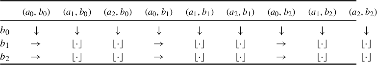
The definition of the terms in (10.3) ensures that
 $$ \begin{align*} \sum_{b \in \mathtt{B}} W_{\mathtt{A}\mathtt{B}}(b, (a^{\prime}, b^{\prime}); i) = W_{\mathtt{A}\mathtt{B}}((a^{\prime},b^{\prime})) \quad \text{for all } a^{\prime},b^{\prime},i. \end{align*} $$
This will ensure that $W_{\mathtt {A}\mathtt {B}}$
has the correct vertex measure. Note also that, by line (10.2),
$W_{\mathtt {A}\mathtt {B}}$
has the correct vertex measure. Note also that, by line (10.2),
 $$ \begin{align*} \sum_{a^{\prime} \in \mathtt{A}} W_{\mathtt{A}\mathtt{B}}(b, (a^{\prime}, b^{\prime}); i) = W_{\mathtt{B}}(b, b^{\prime}; i) \quad \text{for all } b \in \mathtt{B} \setminus \{b_{0}\} \text{ and } b^{\prime} \in \mathtt{B}. \end{align*} $$
Using this and definition (10.3), we also get
 $$ \begin{align*} \sum_{a^{\prime} \in \mathtt{A}} W_{\mathtt{A}\mathtt{B}}(b_{0}, (a^{\prime}, b^{\prime}); i) &= W_{\mathtt{B}}(b_{0}, b^{\prime}; i). \end{align*} $$
This will ensure that the $\mathtt {B}$
-marginal of
$\mathtt {B}$
-marginal of $W_{\mathtt {A}\mathtt {B}}$
is
$W_{\mathtt {A}\mathtt {B}}$
is $W_{\mathtt {B}}$
.
$W_{\mathtt {B}}$
.
We show now that the half-marginal $W_{\mathtt {A}\mathtt {B}}(\cdot , (\cdot , \cdot ); i)$
is
$W_{\mathtt {A}\mathtt {B}}(\cdot , (\cdot , \cdot ); i)$
is $\ell ^{1}$
-close to
$\ell ^{1}$
-close to $W(\cdot , (\cdot , \cdot ); i)$
by considering separately the contributions to the
$W(\cdot , (\cdot , \cdot ); i)$
by considering separately the contributions to the $\ell ^{1}$
distance from terms defined using equations (10.1), (10.2), and (10.3).
$\ell ^{1}$
distance from terms defined using equations (10.1), (10.2), and (10.3).
(10.1) terms: Each of the terms of $W_{\mathtt {A}\mathtt {B}}$
defined using the floor in equation (10.1) is distance at most
$W_{\mathtt {A}\mathtt {B}}$
defined using the floor in equation (10.1) is distance at most $1/n$
from the corresponding term of W; therefore the total contribution of these terms to the
$1/n$
from the corresponding term of W; therefore the total contribution of these terms to the $\ell ^{1}$
distance is
$\ell ^{1}$
distance is
 $$ \begin{align*} \sum_{\substack{b \in \mathtt{B} \setminus \{b_{0}\} \\ a^{\prime} \in \mathtt{A} \setminus\{a_{0}\}, b^{\prime} \in \mathtt{B} \\ i \in [r]}} \lvert W_{\mathtt{A}\mathtt{B}}(b, (a^{\prime}, b^{\prime}); i) - W(b, (a^{\prime}, b^{\prime}); i) \rvert &\leq \lvert \mathtt{A} \rvert \lvert \mathtt{B} \rvert^{2} r/ n. \end{align*} $$
(10.2) terms: By the triangle inequality,
 $$ \begin{align*} & \lvert W_{\mathtt{A}\mathtt{B}}(b, (a_{0}, b^{\prime}); i) - W(b, (a_{0}, b^{\prime}); i) \rvert \\[4pt] &\quad= \bigg\lvert \bigg(W_{\mathtt{B}}(b, b^{\prime}; i) - \sum_{a^{\prime} \ne a_{0}} W_{\mathtt{A}\mathtt{B}}(b, (a^{\prime}, b^{\prime}); i)\bigg)\\[4pt] &\quad\quad - \bigg( \pi_{\mathtt{B}} W(b, b^{\prime}; i) - \sum_{a^{\prime} \ne a_{0}} W(b, (a^{\prime}, b^{\prime}); i) \bigg) \bigg\rvert \\[4pt] &\quad\leq \lvert W_{\mathtt{B}}(b, b^{\prime}; i) - \pi_{\mathtt{B}} W(b, b^{\prime}; i) \rvert\\[4pt] &\quad\quad + \sum_{a^{\prime} \ne a_{0}} \lvert W_{\mathtt{A}\mathtt{B}}(b, (a^{\prime}, b^{\prime}); i) - W(b, (a^{\prime}, b^{\prime}); i) \rvert. \end{align*} $$
The total contribution of such terms is therefore
 $$ \begin{align*} & \sum_{\substack{b \in \mathtt{B} \setminus \{b_{0}\},\ b^{\prime} \in \mathtt{B} \\ i \in [r]}} \lvert W_{\mathtt{A}\mathtt{B}}(b, (a_{0}, b^{\prime}); i) - W(b, (a_{0}, b^{\prime}); i) \rvert \\ &\quad\leq \overbrace{\sum_{\substack{b \in \mathtt{B} \setminus \{b_{0}\},\ b^{\prime} \in \mathtt{B} \\ i \in [r]}} \lvert W_{\mathtt{B}}(b, b^{\prime}; i) - (\pi_{\mathtt{B}})_{*}W(b, b^{\prime}; i) \rvert}^{\leq d_{1}(W_{\mathtt{B}}, \pi_{\mathtt{B}} W)} \\ &\qquad + \overbrace{\sum_{\substack{b \in \mathtt{B} \setminus \{b_{0}\}\\ a^{\prime} \in \mathtt{A} \setminus \{a_{0}\},\ b^{\prime} \in \mathtt{B} \\ i \in [r]}} \lvert W_{\mathtt{A}\mathtt{B}}(b, (a^{\prime}, b^{\prime}); i) - W(b, (a^{\prime}, b^{\prime}); i) \rvert}^{=\text{contribution from (10.1) terms}} \\ &\quad\leq 2\delta + \lvert \mathtt{A} \rvert \lvert \mathtt{B} \rvert^{2} r /n. \end{align*} $$
(10.3) terms: Again applying the triangle inequality,
 $$ \begin{align*}&\lvert W_{\mathtt{A}\mathtt{B}}(b_{0}, (a, b^{\prime}); i) - W(b_{0}, (a, b^{\prime}); i) \rvert \\ &\quad \leq \lvert W_{\mathtt{A}\mathtt{B}}((a,b^{\prime})) - W((a,b^{\prime})) \rvert\\ &\qquad + \sum_{b \ne b_{0}} \lvert W_{\mathtt{A}\mathtt{B}}(b, (a, b^{\prime}); i) - W(b, (a, b^{\prime}); i) \rvert. \end{align*} $$
Summing over all $a \in \mathtt {A}$
,
$a \in \mathtt {A}$
, $b^{\prime } \in \mathtt {B}$
and
$b^{\prime } \in \mathtt {B}$
and $i \in [r]$
, we see that the total contribution of such terms is bounded by
$i \in [r]$
, we see that the total contribution of such terms is bounded by
 $$ \begin{align*} &\sum_{\substack{a \in \mathtt{A}, b^{\prime} \in \mathtt{B} \\ i \in [r]}} \bigg[\lvert W_{\mathtt{A}\mathtt{B}}((a,b^{\prime})) - W((a,b^{\prime})) \rvert \\&\qquad + \sum_{b \ne b_{0}} \lvert W_{\mathtt{A}\mathtt{B}}(b, (a, b^{\prime}); i) - W(b, (a, b^{\prime}); i) \rvert \bigg] \\ &\quad= \sum_{i \in [r]} \overbrace{\sum_{\substack{a \in \mathtt{A} \\ b \in \mathtt{B}}} \lvert W_{\mathtt{A}\mathtt{B}}((a,b)) - W((a,b)) \rvert}^{\text{vertex measure}}\\ &\qquad + \overbrace{\sum_{\substack{b \in \mathtt{B} \setminus \{b_{0}\} \\ a^{\prime} \in \mathtt{A} \setminus\{a_{0}\},\ b^{\prime} \in \mathtt{B} \\ i \in [r]}} \lvert W_{\mathtt{A}\mathtt{B}}(b, (a^{\prime}, b^{\prime}); i) - W(b, (a^{\prime}, b^{\prime}); i) \rvert}^{\text{(10.1) terms}} \\ &\qquad + \overbrace{\sum_{\substack{b \in \mathtt{B} \setminus \{b_{0}\}, \ b^{\prime} \in \mathtt{B} \\ i \in [r]}} \lvert W_{\mathtt{A}\mathtt{B}}(b, (a_{0}, b^{\prime}); i) - W(b, (a_{0}, b^{\prime}); i) \rvert}^{\text{(10.2) terms}} \\ &\leq r \cdot [ 6 \delta + 4 \lvert \mathtt{A} \rvert \lvert \mathtt{B} \rvert / n ] + [ \lvert \mathtt{A} \rvert \lvert \mathtt{B} \rvert^{2} r / n ] + [ 2\delta + \lvert \mathtt{A} \rvert \lvert \mathtt{B} \rvert^{2} r / n ] \\ &\leq 8 r \delta + 6 \lvert \mathtt{A} \rvert \lvert \mathtt{B} \rvert^{2} r / n. \end{align*} $$
Adding up the contributions of the three types of terms, we see that the $\ell ^{1}$
distance between the half-marginals of W and
$\ell ^{1}$
distance between the half-marginals of W and $W_{\mathtt {A}\mathtt {B}}$
is bounded by
$W_{\mathtt {A}\mathtt {B}}$
is bounded by
 $$ \begin{align*} 10r \delta + 8 \lvert \mathtt{A} \rvert \lvert \mathtt{B} \rvert^{2} r/n. \end{align*} $$
10.2.1 Nonnegativity
Again, the preceding construction does not guarantee that all terms are non-negative. In the following we describe how to correct negativity.
Let $-R/n$
be the sum of all negative terms of the half-marginal. As above, we get
$-R/n$
be the sum of all negative terms of the half-marginal. As above, we get
 $$ \begin{align*} R/n \leq 10r\delta + 7 \lvert \mathtt{A} \rvert \lvert \mathtt{B} \rvert^{2}r/n. \end{align*} $$
Suppose there is some $b_{-} \in B$
,
$b_{-} \in B$
, $(a^{\prime }_{-},b^{\prime }_{-}) \in \mathtt {A} \times \mathtt {B}$
, and
$(a^{\prime }_{-},b^{\prime }_{-}) \in \mathtt {A} \times \mathtt {B}$
, and $i \in [r]$
such that
$i \in [r]$
such that $W_{\mathtt {A}\mathtt {B}}(b_{-}, (a^{\prime }_{-},b^{\prime }_{-}); i) < 0$
. Then
$W_{\mathtt {A}\mathtt {B}}(b_{-}, (a^{\prime }_{-},b^{\prime }_{-}); i) < 0$
. Then $W_{\mathtt {A}\mathtt {B}}(b_{-}, (a^{\prime }_{-},b^{\prime }_{-}); i) \leq -1/n$
. Since
$W_{\mathtt {A}\mathtt {B}}(b_{-}, (a^{\prime }_{-},b^{\prime }_{-}); i) \leq -1/n$
. Since
 $$ \begin{align*} \sum_{a^{\prime} \in \mathtt{A}} W_{\mathtt{A}\mathtt{B}}(b_{-}, (a^{\prime},b^{\prime}_{-}); i) = W_{\mathtt{B}}(b_{-}, b^{\prime}_{-}; i) \geq 0 \end{align*} $$
and
 $$ \begin{align*} \sum_{b \in \mathtt{B}} W_{\mathtt{A}\mathtt{B}}(b, (a^{\prime}_{-},b^{\prime}_{-}); i) = W_{\mathtt{A}\mathtt{B}}((a^{\prime}_{-},b^{\prime}_{-})) \geq 0 \end{align*} $$
there exist $a^{\prime }_{+} \in \mathtt {A}$
and
$a^{\prime }_{+} \in \mathtt {A}$
and $b_{+} \in \mathtt {B}$
such that
$b_{+} \in \mathtt {B}$
such that
 $$ \begin{align*} W_{\mathtt{A}\mathtt{B}}(b_{-}, (a^{\prime}_{+},b^{\prime}_{-}); i) \geq 1/n \quad \text{and} \quad W_{\mathtt{A}\mathtt{B}}(b_{+}, (a^{\prime}_{-},b^{\prime}_{-}); i) \geq 1/n. \end{align*} $$
Decrease both of these terms by $1/n$
, and increase both
$1/n$
, and increase both $W_{\mathtt {A}\mathtt {B}}(b_{-}, (a^{\prime }_{-},b^{\prime }_{-}); i)$
and
$W_{\mathtt {A}\mathtt {B}}(b_{-}, (a^{\prime }_{-},b^{\prime }_{-}); i)$
and $W_{\mathtt {A}\mathtt {B}}(b_{+}, (a^{\prime }_{+},b^{\prime }_{-}); i)$
by
$W_{\mathtt {A}\mathtt {B}}(b_{+}, (a^{\prime }_{+},b^{\prime }_{-}); i)$
by $1/n$
. This moves the half-marginal by
$1/n$
. This moves the half-marginal by $\ell ^{1}$
distance
$\ell ^{1}$
distance $4/n$
:
$4/n$
:
 $$ \begin{align*} \sum_{a^{\prime} \in \mathtt{A}} W_{\mathtt{A}\mathtt{B}}(b, (a^{\prime},b^{\prime}); i) = W_{\mathtt{B}}(b, b^{\prime}; i) \quad \text{and} \quad \sum_{b \in \mathtt{B}} W_{\mathtt{A}\mathtt{B}}(b, (a^{\prime},b^{\prime}); i) = W_{\mathtt{A}\mathtt{B}}((a^{\prime},b^{\prime})). \end{align*} $$
This step must be done at most R times to eliminate all negative entries, so the final half-marginal satisfies
 $$ \begin{align*} &\sum_{i \in [r]} \sum_{b \in \mathtt{B}} \sum_{(a^{\prime},b^{\prime}) \in \mathtt{A} \times \mathtt{B}} \lvert W_{\mathtt{A}\mathtt{B}}(b, (a^{\prime},b^{\prime}); i) - W(b, (a^{\prime},b^{\prime}); i) \rvert\\ &\quad\leq (10r\delta + 8 \lvert \mathtt{A} \rvert \lvert \mathtt{B} \rvert^{2}r/n) + R\cdot 4/n \leq 50r\delta + 36 \lvert \mathtt{A} \rvert \lvert \mathtt{B} \rvert^{2}r/n. \end{align*} $$
10.3 The edge measure
Finally, we define the edge measure of $W_{\mathtt {A}\mathtt {B}}$
by
$W_{\mathtt {A}\mathtt {B}}$
by
 $$ \begin{align} \kern-94pt W_{\mathtt{A}\mathtt{B}}( (a, b), (a^{\prime}, b^{\prime}); i) &= \frac{1}{n} \lfloor {n \cdot W((a, b), (a^{\prime}, b^{\prime}); i)} \rfloor\nonumber\\ &\quad \text{for } a \ne a_{0} \text{ and } (a^{\prime},b^{\prime}) \ne (a_{0}, b_{0}), \end{align} $$
 $$ \begin{align} \kern-33pt W_{\mathtt{A}\mathtt{B}}( (a_{0}, b), (a^{\prime}, b^{\prime}); i) &= W_{\mathtt{A}\mathtt{B}}(b, (a^{\prime}, b^{\prime}); i) - \sum_{a \ne a_{0}} W_{\mathtt{A}\mathtt{B}}((a, b), (a^{\prime}, b^{\prime}); i)\nonumber\\ &\quad \text{for } (a^{\prime},b^{\prime}) \ne (a_{0}, b_{0}), \end{align} $$
 $$ \begin{align} W_{\mathtt{A}\mathtt{B}}((a, b), (a_{0}, b_{0}); i) = W_{\mathtt{A}\mathtt{B}}((a, b)) - \sum_{(a^{\prime},b^{\prime}) \ne (a_{0},b_{0})} W_{\mathtt{A}\mathtt{B}}((a, b), (a^{\prime}, b^{\prime}); i). \end{align} $$
See Table 3.
Table 3 A diagram of how the edge measure $W_{\mathtt {A}\mathtt {B}}((\cdot ,\cdot ), (\cdot , \cdot ); i)$
is chosen if
$W_{\mathtt {A}\mathtt {B}}((\cdot ,\cdot ), (\cdot , \cdot ); i)$
is chosen if $\mathtt {A} = \{a_{0}, a_{1}, a_{2}\}$
and
$\mathtt {A} = \{a_{0}, a_{1}, a_{2}\}$
and $\mathtt {B} = \{b_{0}, b_{1}, b_{2}\}$
. First obtain the entries marked
$\mathtt {B} = \{b_{0}, b_{1}, b_{2}\}$
. First obtain the entries marked $\lfloor \cdot \rfloor $
by rounding down entries of W. Then choose entries marked
$\lfloor \cdot \rfloor $
by rounding down entries of W. Then choose entries marked $\downarrow $
according to equation (10.5), which ensures that the
$\downarrow $
according to equation (10.5), which ensures that the $\mathtt {B}$
half-marginal is the one chosen above. Then choose entries marked
$\mathtt {B}$
half-marginal is the one chosen above. Then choose entries marked $\rightarrow $
according to equation (10.6), which ensures that the vertex measure is the one chosen above.
$\rightarrow $
according to equation (10.6), which ensures that the vertex measure is the one chosen above.

It follows from this definition that $W_{\mathtt {A}\mathtt {B}}$
is a (signed) weight with
$W_{\mathtt {A}\mathtt {B}}$
is a (signed) weight with $\mathtt {B}$
-marginal
$\mathtt {B}$
-marginal $W_{\mathtt {B}}$
.
$W_{\mathtt {B}}$
.
We now check that $W_{\mathtt {A}\mathtt {B}}$
is
$W_{\mathtt {A}\mathtt {B}}$
is $\ell ^{1}$
-close to W. We consider separately the contribution to the
$\ell ^{1}$
-close to W. We consider separately the contribution to the $\ell ^{1}$
distance of terms defined in equations (10.4), (10.5), and (10.6).
$\ell ^{1}$
distance of terms defined in equations (10.4), (10.5), and (10.6).
(10.4) terms: Each term of $W_{\mathtt {A}\mathtt {B}}$
defined using the floor function in equation (10.4) is distance at most
$W_{\mathtt {A}\mathtt {B}}$
defined using the floor function in equation (10.4) is distance at most $1/n$
from the corresponding W term. The total contribution of these terms to the
$1/n$
from the corresponding W term. The total contribution of these terms to the $\ell ^{1}$
distance is therefore at most
$\ell ^{1}$
distance is therefore at most $\lvert \mathtt {A} \rvert ^{2} \lvert \mathtt {B} \rvert ^{2} r/n$
.
$\lvert \mathtt {A} \rvert ^{2} \lvert \mathtt {B} \rvert ^{2} r/n$
.
(10.5) terms: Applying the triangle inequality to terms defined in equation (10.5),
 $$ \begin{align*} & \lvert W_{\mathtt{A}\mathtt{B}}( (a_{0}, b), (a^{\prime}, b^{\prime}); i) - W( (a_{0}, b), (a^{\prime}, b^{\prime}); i) \rvert \\ &\quad\leq \lvert W_{\mathtt{A}\mathtt{B}}(b, (a^{\prime}, b^{\prime}); i) -W(b, (a^{\prime}, b^{\prime}); i) \rvert \\ &\qquad + \sum_{a \ne a_{0}} \lvert W_{\mathtt{A}\mathtt{B}}((a, b), (a^{\prime}, b^{\prime}); i) - W((a, b), (a^{\prime}, b^{\prime}); i) \rvert \\ &\quad\leq \lvert W_{\mathtt{A}\mathtt{B}}(b, (a^{\prime}, b^{\prime}); i) -W(b, (a^{\prime}, b^{\prime}); i) \rvert + \lvert \mathtt{A} \rvert/n. \end{align*} $$
By the $\ell ^{1}$
bound on the distance between the half-marginals, the total contribution of all such terms is therefore at most
$\ell ^{1}$
bound on the distance between the half-marginals, the total contribution of all such terms is therefore at most
 $$ \begin{align*} &\sum_{i \in [r]} \sum_{b} \sum_{(a^{\prime},b^{\prime}) \ne (a_{0}, b_{0})} ( \lvert W_{\mathtt{A}\mathtt{B}}(b, (a^{\prime}, b^{\prime}); i) -W(b, (a^{\prime}, b^{\prime}); i) \rvert + \lvert \mathtt{A} \rvert/n ) \\ &\quad\leq [50r\delta + 36 \lvert \mathtt{A} \rvert^{2}\lvert \mathtt{B} \rvert^{2} r / n] + \lvert \mathtt{A} \rvert^{2} \lvert \mathtt{B} \rvert^{2} r / n \\ &\quad= 50r\delta + 37 \lvert \mathtt{A} \rvert^{2}\lvert \mathtt{B} \rvert^{2} r / n. \end{align*} $$
(10.6) terms: Applying the triangle inequality to terms defined in equation (10.6),
 $$ \begin{align*} & \lvert W_{\mathtt{A}\mathtt{B}}((a, b), (a_{0}, b_{0}); i) - W_{\mathtt{A}\mathtt{B}}((a, b), (a_{0}, b_{0}); i) \rvert \\ &\quad\leq \lvert W_{\mathtt{A}\mathtt{B}}((a, b)) - W((a, b)) \rvert\\ &\qquad + \sum_{(a^{\prime},b^{\prime}) \ne (a_{0},b_{0})} \lvert W_{\mathtt{A}\mathtt{B}}((a, b), (a^{\prime}, b^{\prime}); i) - W((a, b), (a^{\prime}, b^{\prime}); i) \rvert. \end{align*} $$
Therefore the total contribution of all such terms is
 $$ \begin{align*} & \sum_{i \in [r]} \sum_{a,b} \lvert W_{\mathtt{A}\mathtt{B}}((a, b), (a_{0}, b_{0}); i) - W_{\mathtt{A}\mathtt{B}}((a, b), (a_{0}, b_{0}); i) \rvert \\ &\quad= \sum_{i \in [r]} \sum_{a,b} \bigg[ \lvert W_{\mathtt{A}\mathtt{B}}((a,b)) - W((a,b)) \rvert \\ &\quad\quad + \sum_{(a^{\prime},b^{\prime}) \ne (a_{0},b_{0})} \lvert W_{\mathtt{A}\mathtt{B}}((a, b), (a^{\prime}, b^{\prime}); i) - W((a, b), (a^{\prime}, b^{\prime}); i) \rvert \bigg] \\ &\quad= \overbrace{\sum_{i \in [r]} \sum_{a,b} \lvert W_{\mathtt{A}\mathtt{B}}((a,b)) - W((a,b)) \rvert}^{\text{vertex measure}} \\ &\quad\quad + \overbrace{\sum_{i \in [r]} \sum_{a \ne a_{0}}\sum_{b}\sum_{(a^{\prime},b^{\prime}) \ne (a_{0},b_{0})} \lvert W_{\mathtt{A}\mathtt{B}}((a, b), (a^{\prime}, b^{\prime}); i) - W((a, b), (a^{\prime}, b^{\prime}); i) \rvert}^{\text{(10.4) terms}} \\ &\quad\quad + \overbrace{\sum_{i \in [r]} \sum_{b}\sum_{(a^{\prime},b^{\prime}) \ne (a_{0},b_{0})} \lvert W_{\mathtt{A}\mathtt{B}}((a_{0}, b), (a^{\prime}, b^{\prime}); i) - W((a_{0}, b), (a^{\prime}, b^{\prime}); i) \rvert}^{\text{(10.5) terms}} \bigg] \\ &\quad\leq r \cdot [6 \delta + 3 \lvert \mathtt{A} \rvert \lvert \mathtt{B} \rvert/n ] + [ \lvert \mathtt{A} \rvert^{2}\lvert \mathtt{B} \rvert^{2} r / n ] + [ 50 r\delta + 37 \lvert \mathtt{A} \rvert^{2}\lvert \mathtt{B} \rvert^{2} r / n ] \\ &\quad\leq 56 r\delta + 41 \lvert \mathtt{A} \rvert^{2}\lvert \mathtt{B} \rvert^{2}r/n. \end{align*} $$
Summing up the contributions from terms of all three types, we get that
 $$ \begin{align*} d_{1}(W_{\mathtt{A}\mathtt{B}}, W) \leq 106 r\delta + 79 \lvert \mathtt{A} \rvert^{2}\lvert \mathtt{B} \rvert^{2}r/n. \end{align*} $$
10.3.1 Nonnegativity
We can modify a solution with negative entries to get a non-negative one similarly to above. Let $-R/n$
be the sum of all negative entries; then
$-R/n$
be the sum of all negative entries; then
 $$ \begin{align*} R/n \leq 106 r\delta + 78 \lvert \mathtt{A} \rvert^{2}\lvert \mathtt{B} \rvert^{2}r/n. \end{align*} $$
Suppose there is some entry
 $$ \begin{align*} W_{\mathtt{A}\mathtt{B}}((a_{-}, b_{-}), (a^{\prime}_{-}, b^{\prime}_{-}); i) \leq -1/n. \end{align*} $$
We want to increment this term by $1/n$
without affecting the vertex measure or the
$1/n$
without affecting the vertex measure or the $\mathtt {B}$
marginal. Since
$\mathtt {B}$
marginal. Since
 $$ \begin{align*} \sum_{(a^{\prime},b^{\prime}) \in \mathtt{A} \times \mathtt{B}} W_{\mathtt{A}\mathtt{B}}((a_{-}, b_{-}), (a^{\prime}, b^{\prime}); i) = W_{\mathtt{A}\mathtt{B}}((a_{-}, b_{-})) \geq 0 \end{align*} $$
there exists some $(a^{\prime }_{+}, b^{\prime }_{+}) \in \mathtt {A} \times \mathtt {B}$
such that
$(a^{\prime }_{+}, b^{\prime }_{+}) \in \mathtt {A} \times \mathtt {B}$
such that $W_{\mathtt {A}\mathtt {B}}((a_{-}, b_{-}), (a^{\prime }_{+}, b^{\prime }_{+}); i) \geq 1/n$
; similarly, since
$W_{\mathtt {A}\mathtt {B}}((a_{-}, b_{-}), (a^{\prime }_{+}, b^{\prime }_{+}); i) \geq 1/n$
; similarly, since
 $$ \begin{align*} \sum_{a \in A} W_{\mathtt{A}\mathtt{B}}((a, b_{-}), (a^{\prime}, b^{\prime}_{-}); i) = W_{\mathtt{A}\mathtt{B}}(b_{-}, (a^{\prime}_{-},b^{\prime}_{-}); i) \geq 0 \end{align*} $$
there exists some $a_{+}$
such that
$a_{+}$
such that $W_{\mathtt {A}\mathtt {B}}((a_{+}, b_{-}), (a^{\prime }_{-}, b^{\prime }_{-}); i) \geq 1/n$
. Increase
$W_{\mathtt {A}\mathtt {B}}((a_{+}, b_{-}), (a^{\prime }_{-}, b^{\prime }_{-}); i) \geq 1/n$
. Increase
 $$ \begin{align*} W_{\mathtt{A}\mathtt{B}}((a_{-}, b_{-}), (a^{\prime}_{-}, b^{\prime}_{-}); i) \quad \text{and} \quad W_{\mathtt{A}\mathtt{B}}((a_{+}, b_{-}), (a^{\prime}_{+}, b^{\prime}_{+}); i) \end{align*} $$
by $1/n$
, and decrease
$1/n$
, and decrease
 $$ \begin{align*} W_{\mathtt{A}\mathtt{B}}((a_{-}, b_{-}), (a^{\prime}_{+}, b^{\prime}_{+}); i) \quad \text{and} \quad W_{\mathtt{A}\mathtt{B}}((a_{+}, b_{-}), (a^{\prime}_{-}, b^{\prime}_{-}); i) \end{align*} $$
by $1/n$
. This moves the weight by
$1/n$
. This moves the weight by $\ell ^{1}$
distance
$\ell ^{1}$
distance $4/n$
.
$4/n$
.
Since R is the maximum number of times we need to do this before there are no more negative entries, the final weight satisfies
 $$ \begin{align*} d_{1}(W_{\mathtt{A}\mathtt{B}}, W) \leq 106 r\delta + 79 \lvert \mathtt{A} \rvert^{2}\lvert \mathtt{B} \rvert^{2}r/n + 4R/n \leq 530 r\delta + 391 \lvert \mathtt{A} \rvert^{2}\lvert \mathtt{B} \rvert^{2}r/n. \end{align*} $$
To simplify, we write
 $$ \begin{align*} d_{1}(W_{\mathtt{A}\mathtt{B}}, W) \leq 530r ( \delta + \lvert \mathtt{A} \times \mathtt{B} \rvert^{2}/n) , \end{align*} $$
or
 $$ \begin{align*} d(W_{\mathtt{A}\mathtt{B}}, W) \leq 265 r( \delta + \lvert \mathtt{A} \times \mathtt{B} \rvert^{2}/n). \end{align*} $$
Acknowledgements
Thanks go to Tim Austin for suggesting that results like Theorems B and C should hold, for many helpful discussions, and for providing comments on earlier drafts. Thanks also go to Ben Hayes for sharing helpful references to the operator algebras literature, and to Lewis Bowen and Brandon Seward for helpful conversations. Thanks go to an anonymous referee for many helpful comments on an earlier draft. This material is based upon work supported by the National Science Foundation under grant no. DMS-1855694.


 Open access