


1. Introduction
Marine ice sheets, such as the West Antarctic ice sheet, are continental ice masses which possess both a grounded and a floating part. These two regions are separated by the so-called grounding line where ice starts floating. There have been several studies in the recent literature aimed at understanding the grounding-line behaviour using numerical simulations, analytical methods or a combination of both. In particular, Schoof (Reference Schoof2007b) and Tsai, Stewart & Thompson (Reference Tsai, Stewart and Thompson2015) have derived, based on simplified mechanical models for marine ice sheets and asymptotic expansions, so-called flux conditions, which allow the flux at the grounding line, i.e. the amount of ice that crosses the grounding line per unit time, to be determined as a function of grounding-line thickness. The stability of marine ice-sheet systems can then be studied, and it has been found that, under certain assumptions, their dynamical behaviour in these simplified mechanical models can be described in terms of saddle-node bifurcations and hysteresis (Schoof Reference Schoof2007a, Reference Schoof2012).
Schoof (Reference Schoof2007b) and Tsai et al. (Reference Tsai, Stewart and Thompson2015) considered two friction laws: the Weertman friction law, in which the magnitude of basal friction is proportional to a power of the basal velocity, and the Coulomb friction law, in which basal friction depends on a yield stress proportional to an effective pressure between the ice sheet and the underlying bedrock. Their work has been extended to more complex configurations including the impact of buttressing, which appears for three-dimensional ice sheets (Schoof, Davis & Popa Reference Schoof, Davis and Popa2017; Haseloff & Sergienko Reference Haseloff and Sergienko2018, Reference Haseloff and Sergienko2022; Pegler Reference Pegler2018a,Reference Peglerb; Sergienko Reference Sergienko2022a), the regime of low driving and basal stress (Sergienko & Wingham Reference Sergienko and Wingham2019) and the impact of non-negligeable bed gradients (Sergienko & Wingham Reference Sergienko and Wingham2022). A current research topic is the study of more complex friction laws (Sergienko & Haseloff Reference Sergienko and Haseloff2023). This research is motivated by the observation that the behaviour of marine ice sheets in long-term numerical simulations is significantly influenced by the friction law that is used, even if the starting configuration can be similar if one tunes adequately the friction coefficients (Brondex et al. Reference Brondex, Gagliardini, Gillet-Chaulet and Durand2017).
In this paper, we derive flux conditions for a general class of friction models related to the Budd friction law, which includes dependence on the basal velocity and on effective pressure. Modelling effective pressure is a challenging topic, and complex hydrology models can be coupled to the ice-sheet model (Hewitt Reference Hewitt2013; Werder et al. Reference Werder, Hewitt, Schoof and Flowers2013; Bueler & van Pelt Reference Bueler and van Pelt2015). Here, we consider two different effective-pressure models that are elementary. The first one is associated with a perfectly permeable bed, similar to the effective-pressure model used in Tsai et al. (Reference Tsai, Stewart and Thompson2015). The second one considers a linear dependence between the effective pressure and the ice thickness, which is frequent in numerical simulations of ice sheets (Bueler & Brown Reference Bueler and Brown2009; Martin et al. Reference Martin, Winkelmann, Haseloff, Albrecht, Bueler, Khroulev and Levermann2011). The derivation of the flux conditions leads to a problem that is formulated in terms of a dynamical system. We provide insight into the existence and uniqueness of a solution to this problem. We propose a numerical solution strategy for obtaining the value of a numerical factor appearing in this system. We also consider hybrid friction laws that are similar to the ones considered in Schoof (Reference Schoof2005, Reference Schoof2010), Gagliardini et al. (Reference Gagliardini, Cohen, Råback and Zwinger2007) and Zoet & Iverson (Reference Zoet and Iverson2020). Instead of allowing only friction coefficients to be tuned, these friction laws can represent different regimes which can be triggered where certain physical conditions are met, e.g. friction has a plastic behaviour near the grounding line. The derivation of flux conditions for hybrid friction laws is challenging because they introduce additional parameters whose magnitude is not necessarily small.
This paper is structured as follows. First, in § 2, the mathematical problem associated with the mechanical behaviour of marine ice sheets is described. Then, in § 3, we show that the approach adopted in Schoof (Reference Schoof2007b) and Tsai et al. (Reference Tsai, Stewart and Thompson2015) can be generalised to the Budd friction law in combination with two different effective-pressure models. Using asymptotic developments, we also provide a justification for the existence and uniqueness of a solution to the resulting leading-order dynamical system. In § 4, we generalise our results to hybrid friction laws similar to the one described in Schoof (Reference Schoof2005) based on a parametrisation of the flux condition. In § 5, we discuss the validity of the assumptions made to derive the flux conditions, and we propose explicit expressions that can be used to take into account effects that have been neglected in the initial derivation. In § 6, the flux conditions are compared with numerical simulations. Finally, in § 7, we discuss our results.
2. Problem formulation
We consider the evolution of an isothermal marine ice sheet using a flowline model known as the shallow-shelf approximation (Morland Reference Morland1987; MacAyeal Reference MacAyeal1989). Such a model is suited for rapidly sliding ice sheets. Vertical shear in the ice is then neglected, and the vertical normal stress is cryostatic. We assume that the ice sheet is in a steady state. For a two-dimensional geometry, the solution to the flowline model consists of two functions defined over an interval  $\varOmega = (0, x_{c})$: the thickness $h: \varOmega \rightarrow \mathbb {R}^+$ and the horizontal velocity $u: \varOmega \rightarrow \mathbb {R}$. The position $x=x_{c}$ corresponds to a calving front, where icebergs detach from the marine ice sheet. For simplicity, we consider a fixed calving-front position. In general, the domain $\varOmega$ contains both a grounded and a floating portion, denoted respectively by $\varOmega _{g}$ and $\varOmega _{f}$. If it exists and is unique, the point where the ice transitions from a grounded to a floating configuration is known as the grounding line and is denoted here by
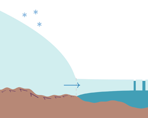
  $x_{gl}$. This position is itself an unknown of the problem. A schematic representation of such an ice-sheet geometry is shown in figure 1.

Figure 1. Schematic representation of the ice-sheet geometry. The unknowns are the grounding-line position  $x_{gl}$, the ice thickness $h=h(x)$ and the horizontal velocity $u=u(x)$. The bed is characterised by a prescribed elevation $b=b(x)$. We also assume that the calving-front position $x_{c}$ is known.
2.1. Governing equations
2.1.1. Multi-domain formulation
Let us denote by  $({h} _{g}, u_{g})$ and $(h_{f}, u_{f})$ the values taken by the functions $(h, u)$ on the grounded portion $\varOmega _{g}$ and the floating portion $\varOmega _{f}$ of the domain $\varOmega$, respectively. With these notations, the governing equations read as follows in the grounded portion:
 \begin{equation}
\left\{ \begin{gathered}
\quad\quad\quad\quad\quad\quad\quad\quad\quad\quad\quad\dfrac{\mathrm{d}}{\mathrm{d}\kern 0.06em x}(u_{g} {h}_{g}) = a, &\quad
\text{in } \varOmega_{g},\\
2 A^{-{1}/{n}} \dfrac{\mathrm{d}}{\mathrm{d}\kern 0.06em x}\left( {h}_{g}
\left\vert \dfrac{\mathrm{d} u_{g}}{\mathrm{d}\kern 0.06em x}
\right\vert^{({1}/{n})-1}\dfrac{\mathrm{d} u_{g}}{\mathrm{d}\kern 0.06em x}\right) - \tau_{b} \phantom{=0,} &\nonumber\\ \quad-
\varLambda {h}_{g}\vert u_{g} \vert^{m-1}u_{g} = \rho
g {h}_{g} \dfrac{\mathrm{d}}{\mathrm{d}\kern 0.06em x}(b + {h}_{g}),
&\quad \text{in } \varOmega_{g}.
\end{gathered}\right.\end{equation}
\begin{equation}
\left\{ \begin{gathered}
\quad\quad\quad\quad\quad\quad\quad\quad\quad\quad\quad\dfrac{\mathrm{d}}{\mathrm{d}\kern 0.06em x}(u_{g} {h}_{g}) = a, &\quad
\text{in } \varOmega_{g},\\
2 A^{-{1}/{n}} \dfrac{\mathrm{d}}{\mathrm{d}\kern 0.06em x}\left( {h}_{g}
\left\vert \dfrac{\mathrm{d} u_{g}}{\mathrm{d}\kern 0.06em x}
\right\vert^{({1}/{n})-1}\dfrac{\mathrm{d} u_{g}}{\mathrm{d}\kern 0.06em x}\right) - \tau_{b} \phantom{=0,} &\nonumber\\ \quad-
\varLambda {h}_{g}\vert u_{g} \vert^{m-1}u_{g} = \rho
g {h}_{g} \dfrac{\mathrm{d}}{\mathrm{d}\kern 0.06em x}(b + {h}_{g}),
&\quad \text{in } \varOmega_{g}.
\end{gathered}\right.\end{equation}
Equation (2.1a) is a mass-conservation equation, stating that the flux variation of the ice flow must be exactly compensated by the net mass accumulation rate  $a$. Equation (2.1b) is a momentum-conservation equation and establishes a balance between the divergence of membrane stress, the friction stress, the lateral-drag stress and the gravitational stress. The factor $A$ and the exponent $n$ are ice viscosity parameters associated with the Glen flow law (usually, $n=3$), $\varLambda$ and m are lateral-drag coefficients, $\rho$ is the ice density, $\rho _{w}$ is the water density, $g$ is the gravitational acceleration and $b=b(x)$ is the prescribed elevation of the underlying bedrock. The models used for the friction stress $\tau _{b}=\tau _{b}(h, u)$ are described in the next section. While we do not explicitly consider lateral drag in the present study, we do include it in the problem formulation, as it allows for an easier comparison with the other results from the literature.
In the floating portion, friction with the ocean and the air is neglected, leading to the following:
 \begin{equation}
\left\{ \begin{gathered}
\quad\quad\quad\quad\quad\quad\quad\quad\quad\quad\quad\quad\quad\quad\quad\quad\dfrac{\mathrm{d}}{\mathrm{d}\kern 0.06em x}(u_{f} h_{f}) = a, &\quad
\text{in } \varOmega_{f},\\ 2
A^{-{1}/{n}} \dfrac{\mathrm{d}}{\mathrm{d}\kern 0.06em x}\left( h_{f}
\left\vert \dfrac{\mathrm{d} u_{f}}{\mathrm{d}\kern 0.06em x}
\right\vert^{({1}/{n})-1}\dfrac{\mathrm{d} u_{f}}{\mathrm{d}\kern 0.06em x}\right) -\varLambda h_{f}\vert u_{f} \vert^{m-1}u_{f}
\phantom{=0,} & \nonumber\\
\quad\quad\quad\quad\quad\quad\quad\quad\quad\quad\quad\quad= \rho\left(1 -
\dfrac{\rho}{\rho_{w}}\right) g h_{f} \dfrac{\mathrm{d}
h_{f}}{\mathrm{d}\kern 0.06em x},&\quad \text{in } \varOmega_{f}.
\end{gathered}\right.\end{equation}
\begin{equation}
\left\{ \begin{gathered}
\quad\quad\quad\quad\quad\quad\quad\quad\quad\quad\quad\quad\quad\quad\quad\quad\dfrac{\mathrm{d}}{\mathrm{d}\kern 0.06em x}(u_{f} h_{f}) = a, &\quad
\text{in } \varOmega_{f},\\ 2
A^{-{1}/{n}} \dfrac{\mathrm{d}}{\mathrm{d}\kern 0.06em x}\left( h_{f}
\left\vert \dfrac{\mathrm{d} u_{f}}{\mathrm{d}\kern 0.06em x}
\right\vert^{({1}/{n})-1}\dfrac{\mathrm{d} u_{f}}{\mathrm{d}\kern 0.06em x}\right) -\varLambda h_{f}\vert u_{f} \vert^{m-1}u_{f}
\phantom{=0,} & \nonumber\\
\quad\quad\quad\quad\quad\quad\quad\quad\quad\quad\quad\quad= \rho\left(1 -
\dfrac{\rho}{\rho_{w}}\right) g h_{f} \dfrac{\mathrm{d}
h_{f}}{\mathrm{d}\kern 0.06em x},&\quad \text{in } \varOmega_{f}.
\end{gathered}\right.\end{equation}
Finally, continuity conditions are added at the interface between the regions:
 \begin{align} {h}_{g} =h_{f}, \quad
u_{g}= u_{f}, \quad 2 A^{-{1}/{n}} {h}_{g} \left\vert
\dfrac{\mathrm{d} u_{g}}{\mathrm{d}\kern 0.06em x}
\right\vert^{({1}/{n})-1}\dfrac{\mathrm{d}
u_{g}}{\mathrm{d}\kern 0.06em x}= 2 A^{-{1}/{n}} h_{f}
\left\vert \dfrac{\mathrm{d} u_{f}}{\mathrm{d}\kern 0.06em
x} \right\vert^{({1}/{n})-1}\dfrac{\mathrm{d}
u_{f}}{\mathrm{d}\kern 0.06em x}\quad \text{on }
\varSigma.
\end{align}
\begin{align} {h}_{g} =h_{f}, \quad
u_{g}= u_{f}, \quad 2 A^{-{1}/{n}} {h}_{g} \left\vert
\dfrac{\mathrm{d} u_{g}}{\mathrm{d}\kern 0.06em x}
\right\vert^{({1}/{n})-1}\dfrac{\mathrm{d}
u_{g}}{\mathrm{d}\kern 0.06em x}= 2 A^{-{1}/{n}} h_{f}
\left\vert \dfrac{\mathrm{d} u_{f}}{\mathrm{d}\kern 0.06em
x} \right\vert^{({1}/{n})-1}\dfrac{\mathrm{d}
u_{f}}{\mathrm{d}\kern 0.06em x}\quad \text{on }
\varSigma.
\end{align}
The portions  $\varOmega _{g}$ and $\varOmega _{f}$ and their interface $\varSigma$ are defined by a flotation condition:
 \begin{equation}
\left\{ \begin{gathered}
&\varOmega_{g} = \{x \in \varOmega: \rho g h > \rho_{w} g \langle -b\rangle\},\\
&\varOmega_{f} = \{x \in \varOmega: \rho g h < \rho_{w} g \langle -b\rangle\},\\
&\varSigma = \bar{\varOmega}_{g} \cap \bar{\varOmega}_{f}.\quad\quad\quad\quad\quad\quad\quad\quad
\end{gathered}\right.\end{equation}
\begin{equation}
\left\{ \begin{gathered}
&\varOmega_{g} = \{x \in \varOmega: \rho g h > \rho_{w} g \langle -b\rangle\},\\
&\varOmega_{f} = \{x \in \varOmega: \rho g h < \rho_{w} g \langle -b\rangle\},\\
&\varSigma = \bar{\varOmega}_{g} \cap \bar{\varOmega}_{f}.\quad\quad\quad\quad\quad\quad\quad\quad
\end{gathered}\right.\end{equation}
The symbol  $\langle {\cdot } \rangle = \max ({\cdot }, 0)$ corresponds to the Macaulay brackets. Hence, the grounded portion includes both the parts where the bedrock lies above the sea level (i.e. where $\langle - b\rangle = 0$), as well as the parts where the bedrock lies below the sea level, but where there is too much ice for it to be floating (i.e. where $\rho g h > -\rho _{w} g b$).
In the simplest configuration, such as the one shown in figure 1, the grounded and floating portions can be written as open sets  $\varOmega _{g} = (0, x_{gl})$ and $\varOmega _{g} = (x_{gl}, x_{c})$, so that the grounded-line position can be properly defined as the unique element of $\varSigma$: $\varSigma = \{ x_{gl}\}$. We note that, in general, the geometry might be more complex. For example, there could be several isolated points on which the ice sheet switches from a grounded to a floating position and vice versa, leading to multiple grounding lines. A more exotic configuration, not considered here, is the one described by Pegler (Reference Pegler2018a) with the so-called marginal-flotation zones. In that case, the interface $\varSigma$ becomes a set of its own, i.e. the grounding-line width becomes finite.
2.1.2. Boundary conditions
At  $x=0$, we assume the ice to be sufficiently slow so that it is virtually motionless (this could also correspond to a symmetry condition):
 \begin{equation} u = 0, \quad \text{at } x = 0. \end{equation}
At the calving front, equilibrium between the horizontal stress in the ice and the ocean water pressure yields the following Neumann boundary condition:
 \begin{equation} 2A^{-{1}/{n}} \left\vert \dfrac{\mathrm{d} u}{\mathrm{d}\kern 0.06em x}\right\vert^{({1}/{n})-1}\dfrac{\mathrm{d} u}{\mathrm{d}\kern 0.06em x} = \dfrac{1}{2}\rho \left(1 - \dfrac{\rho}{\rho_{w}}\right)gh, \quad \text{at } x = x_{c}. \end{equation}
 Actually, if one considers an ice shelf without lateral drag and restricts the domain to the grounded part  $\varOmega _{g}$ only, which we will do in this study, then this boundary condition can still be used, i.e.
 \begin{equation} 2A^{-{1}/{n}} \left\vert \dfrac{\mathrm{d} u}{\mathrm{d}\kern 0.06em x}\right\vert^{({1}/{n})-1}\dfrac{\mathrm{d} u}{\mathrm{d}\kern 0.06em x} = \dfrac{1}{2}\rho \left(1 - \dfrac{\rho}{\rho_{w}}\right)gh, \quad \text{at } x = x_{gl}. \end{equation}
Indeed, (2.2b) with  $\varLambda = 0$ implies that the quantity
 \begin{equation} \left[2A^{-{1}/{n}} h \left\vert \dfrac{\mathrm{d} u}{\mathrm{d}\kern 0.06em x}\right\vert^{({1}/{n})-1}\dfrac{\mathrm{d} u}{\mathrm{d}\kern 0.06em x} - \dfrac{1}{2}\rho \left(1 - \dfrac{\rho}{\rho_{w}}\right)gh\right] \end{equation}
is conserved through the ice shelf.
2.2. Friction laws
2.2.1. Power-law friction laws
The simplest friction law is the Weertman friction law, for which  $\tau _{b}$ is proportional to $\vert u \vert ^p$ with $p > 0$ (Weertman Reference Weertman1957). Usually, $p=1/3$ is chosen. To take into account effective pressure, one can use the so-called Budd friction law (Budd, Keage & Blundy Reference Budd, Keage and Blundy1979) for which
 \begin{equation} \tau_{b} = C N^{q}\,\vert u \vert^{p-1} u, \end{equation}
with  $C$ a friction coefficient, $N$ an effective pressure and $p,q \ge 0$. Two elementary effective-pressure models are presented in § 2.2.5. The Budd friction law can be rewritten as a sliding law, i.e. the velocity can be written as a function of the basal friction stress:
 \begin{equation} u = C^{-{1}/{p}}N^{-{q}/{p}} \vert \tau_{b} \vert^{{1}/{p}-1} \tau_{b}. \end{equation}
It can also be noted that the law in (2.9) includes as a particular case the Weertman friction law if one sets  $p = 1/3$ and $q=0$.
2.2.2. Coulomb friction law
A Coulomb behaviour assumes that there is a yield stress  $\tau _{y} = C N$ that must be reached for ice to be sliding:
 \begin{equation}
\left\{ \begin{gathered}
\tau_{b} = C N \text{sgn}(u), &\quad \text{if $\vert u \vert > 0$},\\\quad\quad
\vert\tau_{b}\vert \le C N, &\quad \text{if $u = 0$}.
\end{gathered}\right.\end{equation}
\begin{equation}
\left\{ \begin{gathered}
\tau_{b} = C N \text{sgn}(u), &\quad \text{if $\vert u \vert > 0$},\\\quad\quad
\vert\tau_{b}\vert \le C N, &\quad \text{if $u = 0$}.
\end{gathered}\right.\end{equation}
If the ice velocity is non-zero everywhere, then  $\tau _{b} = C N \text {sgn}(u)$, which formally corresponds to a Budd friction law with $p=0$ and $q=1$. In the rest of this paper, we will always consider this case.
2.2.3. Hybrid friction laws
Tsai et al. (Reference Tsai, Stewart and Thompson2015) have considered a hybrid law that combines the Weertman and Coulomb friction laws:
 \begin{equation} \tau_{b} = \min(A_{s}^{{-}p}\vert u \vert^{p}, {C}N)\,\text{sgn}(u), \end{equation}
with  $A_{s}$ a friction coefficient that controls the onset of the plastic behaviour. Such a law was originally introduced in Schoof (Reference Schoof2010). Smoothed versions have already been studied analytically and numerically (Schoof Reference Schoof2005, Reference Schoof2010; Gagliardini et al. Reference Gagliardini, Cohen, Råback and Zwinger2007). They take the following form:
 \begin{equation} \tau_{b} = C \left( \dfrac{\vert u \vert}{\vert u \vert + A_{s}C^{{1}/{p}}N^{{1}/{p}}}\right)^{p}N\,\text{sgn}(u), \end{equation}
or, by introducing  $u_0 = A_{s}C^{{1}/{p}}N^{{1}/{p}}$,
 \begin{equation} \tau_{b} = C \left( \dfrac{\vert u \vert}{\vert u \vert + u_0}\right)^{p}N\,\text{sgn}(u). \end{equation}
This type of law, which exhibits viscoplastic behaviour, is interesting from a modelling perspective because it can be used to include both form and skin drag, even if these are distinct mechanisms (Minchew & Joughin Reference Minchew and Joughin2020). Form drag is associated with friction induced by ice deformation around obstacles and can be modelled with a power-law friction law, while skin drag is associated with friction induced by shear stress at the ice–bedrock interface, and can be modelled with a Coulomb friction law. Recently, Zoet & Iverson (Reference Zoet and Iverson2015, Reference Zoet and Iverson2020) have shown that such laws are in good agreement with experimental results.
2.2.4. Summary
The friction laws that we will consider in this article are shown in figure 2.

Figure 2. The considered friction models. The same notation  $C$ is used for the friction coefficient in every friction law although those coefficients are not necessarily comparable to one another.
2.2.5. Effective pressure
Modelling effective pressure is complex. The effective pressure can be expected to depend on both the subglacial interface and the subglacial hydrology whose description is an active area of research (Flowers Reference Flowers2015). State-of-the-art hydrology models typically involve sets of partial differential equations that must be coupled with the ice-sheet model itself (Hewitt Reference Hewitt2013; Werder et al. Reference Werder, Hewitt, Schoof and Flowers2013; Bueler & van Pelt Reference Bueler and van Pelt2015). Here, we will limit ourselves to very simple hydrology models that provide an explicit equation for the effective pressure  $N= \rho g h - p_{w}$.
The first elementary effective-pressure model we consider consists in assuming that the bedrock below the ice sheet is perfectly permeable and connected to the nearby ocean, so that  $N = \rho g h - p_{w}$ with $p_{w}$ following a hydrostatic distribution: $p_{w} = \rho _{w} g \langle -b\rangle$. The second elementary effective-pressure model we consider consists in assuming a dependence of $p_{w}$ on the ice-sheet thickness $h$, such as through a linear relation $p_{w} = c \rho g h$, with $c$ a coefficient close to, but smaller than, one. We choose this model for its simplicity, and because similar parametrisations are common in ice-sheet models. For example, Bueler & Brown (Reference Bueler and Brown2009) consider $p_{w} = 0.95 \rho g h (w/w_{c})$, with $w$ the thickness of a subglacial water film and $w_{c}$ a critical value of that thickness. Martin et al. (Reference Martin, Winkelmann, Haseloff, Albrecht, Bueler, Khroulev and Levermann2011) consider $p_{w} = 0.96 \lambda \rho g h$, with $\lambda$ a parameter depending on the bedrock elevation that is such that $0 \le \lambda \le 1$. We acknowledge that such relations are usually used as parametrisations to close models, and they do not necessarily rely on the modelling of a physical phenomenon. For convenience, we name the first type of elementary effective-pressure model N $_\text {A}$ and the second one N $_\text {B}$.
2.3. Dimensionless formulation
We introduce scales  $[x], [h], [u]$, and $[\tau _{b}]$, leading to the dimensionless variables
 \begin{equation} \hat{x} = \dfrac{x}{[x]}, \quad \hat{h} = \dfrac{h}{[h]}, \quad \hat{b} = \dfrac{b}{[h]}, \quad \hat{u} = \dfrac{u}{[u]}, \quad \hat{\tau}_{b} = \dfrac{\tau_{b}}{[\tau_{b}]}, \end{equation}
and to the following dimensionless ratios:
 \begin{equation}
\left\{ \begin{gathered}
\alpha = \dfrac{a}{([u]/[x])[h]}, \quad \beta = \left(\dfrac{\mathrm{d} b}{\mathrm{d}\kern 0.06em x}\right)\dfrac{[x]}{[h]}, \quad \gamma = \dfrac{[\tau_{b}][x]}{\rho g [h]^2},\\
\delta = \dfrac{\rho_{w} - \rho}{\rho_{w}}, \quad \varepsilon = \dfrac{A^{-{1}/{n}}[u]^{{1}/{n}}}{2\rho g [x]^{{1}/{n}}[h]}, \quad \lambda = \dfrac{\varLambda [u]^{m}[x]}{\rho g [h]}.
\end{gathered}\right.\end{equation}
\begin{equation}
\left\{ \begin{gathered}
\alpha = \dfrac{a}{([u]/[x])[h]}, \quad \beta = \left(\dfrac{\mathrm{d} b}{\mathrm{d}\kern 0.06em x}\right)\dfrac{[x]}{[h]}, \quad \gamma = \dfrac{[\tau_{b}][x]}{\rho g [h]^2},\\
\delta = \dfrac{\rho_{w} - \rho}{\rho_{w}}, \quad \varepsilon = \dfrac{A^{-{1}/{n}}[u]^{{1}/{n}}}{2\rho g [x]^{{1}/{n}}[h]}, \quad \lambda = \dfrac{\varLambda [u]^{m}[x]}{\rho g [h]}.
\end{gathered}\right.\end{equation}
These scales and ratios should be characteristic of ice streams. The problem can be further simplified by choosing the scales so that additional constraints on the dimensionless ratios are enforced, e.g. by setting some of them to a unit value. However, we postpone these assumptions to a later stage, where the context will provide justification for them. We also introduce the dimensionless flotation thickness  $\hat {h}_{b}$ as $\hat {h}_{b} = (1-\delta )^{-1} \hat {b}$. With these notations, the governing equations become
 \begin{equation}
\left\{ \begin{gathered}
\quad\quad\quad\quad\quad\quad\quad\quad\quad\quad\quad\quad\quad\quad\quad\quad\quad\quad\quad\quad\quad\quad\dfrac{\mathrm{d}}{\mathrm{d} \hat{x}}(\hat{u}_{g}\,\hat{h}_{g}) = \alpha,\\
4\varepsilon \dfrac{\mathrm{d}}{\mathrm{d} \hat{x}}\left( \hat{h}_{g} \left\vert\dfrac{\mathrm{d} \hat{u}_{g}}{\mathrm{d} \hat{x}} \right\vert^{({1}/{n})-1}\dfrac{\mathrm{d} \hat{u}_{g}}{\mathrm{d} \hat{x}}\right) - \gamma\,\hat{\tau}_{b} - \lambda\,\hat{h}_{g} \vert \hat{u}_{g} \vert^{m-1}\hat{u}_{g} = \hat{h}_{g} \left(\dfrac{\mathrm{d} \hat{h}_{g}}{\mathrm{d} \hat{x}} + \beta\right),
\end{gathered}\right.\end{equation}
\begin{equation}
\left\{ \begin{gathered}
\quad\quad\quad\quad\quad\quad\quad\quad\quad\quad\quad\quad\quad\quad\quad\quad\quad\quad\quad\quad\quad\quad\dfrac{\mathrm{d}}{\mathrm{d} \hat{x}}(\hat{u}_{g}\,\hat{h}_{g}) = \alpha,\\
4\varepsilon \dfrac{\mathrm{d}}{\mathrm{d} \hat{x}}\left( \hat{h}_{g} \left\vert\dfrac{\mathrm{d} \hat{u}_{g}}{\mathrm{d} \hat{x}} \right\vert^{({1}/{n})-1}\dfrac{\mathrm{d} \hat{u}_{g}}{\mathrm{d} \hat{x}}\right) - \gamma\,\hat{\tau}_{b} - \lambda\,\hat{h}_{g} \vert \hat{u}_{g} \vert^{m-1}\hat{u}_{g} = \hat{h}_{g} \left(\dfrac{\mathrm{d} \hat{h}_{g}}{\mathrm{d} \hat{x}} + \beta\right),
\end{gathered}\right.\end{equation}
for  $0 < \hat {x} < \hat {x}_{gl}$,
 \begin{equation}
\hat{h}_{g}
=\hat{h}_{f}, \quad \hat{u}_{g}= \hat{u}_{f}, \quad
\hat{h}_{g} \left\vert \dfrac{\mathrm{d}
\hat{u}_{g}}{\mathrm{d}\kern 0.06em x}
\right\vert^{({1}/{n})-1}\dfrac{\mathrm{d}
\hat{u}_{g}}{\mathrm{d}\kern 0.06em x}= \hat{h}_{f}
\left\vert \dfrac{\mathrm{d} \hat{u}_{f}}{\mathrm{d}\kern
0.06em x} \right\vert^{({1}/{n})-1}\dfrac{\mathrm{d}
\hat{u}_{f}}{\mathrm{d}\kern 0.06em x},
\end{equation}
\begin{equation}
\hat{h}_{g}
=\hat{h}_{f}, \quad \hat{u}_{g}= \hat{u}_{f}, \quad
\hat{h}_{g} \left\vert \dfrac{\mathrm{d}
\hat{u}_{g}}{\mathrm{d}\kern 0.06em x}
\right\vert^{({1}/{n})-1}\dfrac{\mathrm{d}
\hat{u}_{g}}{\mathrm{d}\kern 0.06em x}= \hat{h}_{f}
\left\vert \dfrac{\mathrm{d} \hat{u}_{f}}{\mathrm{d}\kern
0.06em x} \right\vert^{({1}/{n})-1}\dfrac{\mathrm{d}
\hat{u}_{f}}{\mathrm{d}\kern 0.06em x},
\end{equation}
at  $\hat {x} = \hat {x}_{gl}$,
 \begin{equation}
\left\{ \begin{gathered}
\quad\quad\quad\quad\quad\quad\quad\quad\quad\quad\quad\quad\quad\quad\quad\quad\dfrac{\mathrm{d}}{\mathrm{d} \hat{x}}(\hat{u}_{f}\,\hat{h}_{f}) = \alpha,\\
4 \varepsilon\, \dfrac{\mathrm{d}}{\mathrm{d} \hat{x}}\left( \hat{h}_{f} \left\vert\dfrac{\mathrm{d} \hat{u}_{f}}{\mathrm{d} \hat{x}} \right\vert^{({1}/{n})-1}\dfrac{\mathrm{d} \hat{u}_{f}}{\mathrm{d} \hat{x}}\right) - \lambda\,\hat{h}_{f} \vert \hat{u}_{f} \vert^{m-1}\hat{u}_{f} = \delta\,\hat{h}_{f} \dfrac{\mathrm{d} \hat{h}_{f}}{\mathrm{d} \hat{x}},
\end{gathered}\right.\end{equation}
\begin{equation}
\left\{ \begin{gathered}
\quad\quad\quad\quad\quad\quad\quad\quad\quad\quad\quad\quad\quad\quad\quad\quad\dfrac{\mathrm{d}}{\mathrm{d} \hat{x}}(\hat{u}_{f}\,\hat{h}_{f}) = \alpha,\\
4 \varepsilon\, \dfrac{\mathrm{d}}{\mathrm{d} \hat{x}}\left( \hat{h}_{f} \left\vert\dfrac{\mathrm{d} \hat{u}_{f}}{\mathrm{d} \hat{x}} \right\vert^{({1}/{n})-1}\dfrac{\mathrm{d} \hat{u}_{f}}{\mathrm{d} \hat{x}}\right) - \lambda\,\hat{h}_{f} \vert \hat{u}_{f} \vert^{m-1}\hat{u}_{f} = \delta\,\hat{h}_{f} \dfrac{\mathrm{d} \hat{h}_{f}}{\mathrm{d} \hat{x}},
\end{gathered}\right.\end{equation}
for  $\hat {x}_{gl} < \hat {x} < \hat {x}_{c}$, with the following boundary conditions:
 \begin{equation}
\left\{ \begin{gathered}
\quad\quad\quad\quad\quad\quad\hat{u} = 0, & \quad \text{at } \hat{x} = 0,\\
\left\vert\dfrac{\mathrm{d} \hat{u}}{\mathrm{d} \hat{x}} \right\vert^{({1}/{n})-1}\dfrac{\mathrm{d} \hat{u}}{\mathrm{d} \hat{x}} = \dfrac{\delta\hat{h}}{8 \varepsilon}, & \quad \text{at } \hat{x} = \hat{x}_{gl},\\
\quad\quad\quad\quad\quad\quad\hat{h} = \hat{h}_{b}, & \quad \text{at } \hat{x} = \hat{x}_{gl}.
\end{gathered}\right.\end{equation}
\begin{equation}
\left\{ \begin{gathered}
\quad\quad\quad\quad\quad\quad\hat{u} = 0, & \quad \text{at } \hat{x} = 0,\\
\left\vert\dfrac{\mathrm{d} \hat{u}}{\mathrm{d} \hat{x}} \right\vert^{({1}/{n})-1}\dfrac{\mathrm{d} \hat{u}}{\mathrm{d} \hat{x}} = \dfrac{\delta\hat{h}}{8 \varepsilon}, & \quad \text{at } \hat{x} = \hat{x}_{gl},\\
\quad\quad\quad\quad\quad\quad\hat{h} = \hat{h}_{b}, & \quad \text{at } \hat{x} = \hat{x}_{gl}.
\end{gathered}\right.\end{equation}
2.4. Flux conditions
A flux condition is an expression of the grounding-line flux  $q_{gl} \equiv h(x_{gl}) u(x_{gl})$ as a function of the different physical parameters $A, C,\ldots$ that appear in the problem formulation. Such an expression usually takes the form of an approximation that is valid within an asymptotic regime associated with the magnitude of the previously introduced dimensionless ratios. Historically, the first flux condition was derived by Schoof (Reference Schoof2007b) for the Weertman friction law. They considered an unbuttressed ice sheet, i.e. $\lambda = 0$, a scaling and a bed geometry such that $\alpha \sim 1, \gamma \sim 1$ and $\vert \beta \vert \lesssim 1$, and they assumed that $\varepsilon \ll 1$ and $\delta \ll 1$. Tsai et al. (Reference Tsai, Stewart and Thompson2015) derived a flux condition under the same assumptions, but for the Coulomb friction law. They showed that the resulting flux condition was more sensitive compared with the one derived by Schoof (Reference Schoof2007b). The importance of buttressing, i.e. the case $\lambda \neq 0$, was discussed by Pegler (Reference Pegler2016, Reference Pegler2018a,Reference Peglerb), Schoof et al. (Reference Schoof, Davis and Popa2017) and Haseloff & Sergienko (Reference Haseloff and Sergienko2018, Reference Haseloff and Sergienko2022). They showed that taking into account lateral drag could significantly change the dynamics of ice sheets, in particular by modifying the stability criterion that was previously derived for unbuttressed ice sheets (Schoof Reference Schoof2012). The regime of low basal stress, $\gamma \ll 1$, was covered by Sergienko & Wingham (Reference Sergienko and Wingham2019). The same authors also discussed the importance of $\alpha$ and $\beta$, showing that the so-called marine ice-sheet instability hypothesis was not applicable in general (Sergienko Reference Sergienko2022b; Sergienko & Wingham Reference Sergienko and Wingham2022). Schoof et al. (Reference Schoof, Davis and Popa2017) studied the impact that calving laws have on the flux conditions. All these authors, except Tsai et al. (Reference Tsai, Stewart and Thompson2015), have considered the Weertman friction law in their studies. Recently, Sergienko & Haseloff (Reference Sergienko and Haseloff2023) studied the notion of stability of marine ice sheets submitted to a climate forcing for a broad class of friction laws. However, they did not derive flux conditions for the configuration studied in the present paper, which we describe hereafter.
In this paper, we derive flux conditions for the Budd friction law with two elementary effective-pressure models, and show how they can be extended to hybrid friction laws. We will use the same assumptions that were done by Schoof (Reference Schoof2007b) and Tsai et al. (Reference Tsai, Stewart and Thompson2015), namely, we consider an unbuttressed ice sheet ( $\lambda = 0$), scales that are such that $\alpha, \beta$, and $\gamma$ are at most of order $O(1)$, and consider the asymptotic regimes $\varepsilon \ll 1$ and $\delta \ll 1$. We will discuss in a later section the validity of these hypotheses, and we will show how the flux conditions can be modified to remain valid in the event that $\alpha, \beta$, and $\gamma$ are not small or moderate.
3. Generalisation to the Budd friction law
We now proceed to the derivation of a flux condition for the Budd friction law, that is, we consider a friction law belonging to the family of friction laws  $\tau _{b}={C}N ^{q} \vert u \vert ^{p-1} u$, where the effective pressure $N$ obeys one of the two elementary models previously introduced. We assume that $n=3, 0 \le p \le 1/3$ and $0 \le q \le 1$, which holds for commonly used values. We assume that all the variables that appear are constant, except $x$ and the functions $b, h, u$ and $N$, which depend on this coordinate. We base our derivation on the ideas that Schoof (Reference Schoof2007b) and Tsai et al. (Reference Tsai, Stewart and Thompson2015) have developed for the Weertman and the Coulomb friction laws, and we show that they can be extended to the present context.
We introduce the dimensionless effective pressure as  $\hat {N} = N/[N]$ where the scale $[N]$ is related to the scales $[h]$ and $[\tau _{b}]$ as follows:
 \begin{equation}
[N] = \left\{ \begin{array}{@{}ll} \rho g [h] & \quad \text{(N$_\text{A}$ model)}, \\
(1-c) \rho g [h] & \quad \text{(N$_\text{B}$ model)}, \end{array} \right. \quad \text{and} \quad [\tau_{b}] = C [u]^{p} [N]^{q}.
\end{equation}
\begin{equation}
[N] = \left\{ \begin{array}{@{}ll} \rho g [h] & \quad \text{(N$_\text{A}$ model)}, \\
(1-c) \rho g [h] & \quad \text{(N$_\text{B}$ model)}, \end{array} \right. \quad \text{and} \quad [\tau_{b}] = C [u]^{p} [N]^{q}.
\end{equation}
We neglect lateral drag ( $\lambda = 0$) and consider scales that are such that
 \begin{equation} \alpha = 1, \quad \gamma = 1 \quad \text{and} \quad \vert \beta \vert \lesssim 1. \end{equation}
With these considerations, the following problem is obtained:
 \begin{equation}
\left\{ \begin{gathered}
\quad\quad\quad\quad\quad\quad\quad\quad\quad\quad\quad\quad\quad\quad\dfrac{\mathrm{d}}{\mathrm{d} \hat{x}}(\hat{u}\,\hat{h}) =
1, & \quad \text{for } 0 < \hat{x} < \hat{x}_{gl}, \\ 4 \varepsilon
\dfrac{\mathrm{d}}{\mathrm{d} \hat{x}}\left( \hat{h}
\left\vert\dfrac{\mathrm{d} \hat{u}}{\mathrm{d} \hat{x}}
\right\vert^{({1}/{n})-1}\dfrac{\mathrm{d}
\hat{u}}{\mathrm{d} \hat{x}}\right) - (\hat{h} -
1_{\text{A}}\langle{\hat{h}}_{b}\rangle)^{q}\vert\hat{u}\vert^{p-1}\hat{u}
\phantom{=0,} & \nonumber\\\quad\quad\quad\quad\quad\quad\quad\quad\quad\quad\quad\quad\quad - \hat{h}
\left(\dfrac{\mathrm{d} \hat{h} }{\mathrm{d} \hat{x}}+
\beta\right) = 0, & \quad \text{for } 0 < \hat{x} <
\hat{x}_{gl},\\\quad\quad\quad\quad\quad\quad\quad\quad\quad\quad\quad\quad\quad\quad\quad\quad
\hat{u} = 0, & \quad \text{at } \hat{x} = 0,\\\quad\quad\quad\quad\quad\quad\quad\quad\quad\quad\quad
\left\vert\dfrac{\mathrm{d} \hat{u}}{\mathrm{d} \hat{x}} \right\vert^{({1}/{n})-1}\dfrac{\mathrm{d} \hat{u}}{\mathrm{d} \hat{x}} = \dfrac{\delta\hat{h}}{8 \varepsilon}, & \quad \text{at } \hat{x} = \hat{x}_{gl},\\
\quad\quad\quad\quad\quad\quad\quad\quad\quad\quad\quad\quad\quad\quad\quad\quad\hat{h} = \hat{h}_{b}, & \quad \text{at } \hat{x} = \hat{x}_{gl},
\end{gathered}\right.\end{equation}
\begin{equation}
\left\{ \begin{gathered}
\quad\quad\quad\quad\quad\quad\quad\quad\quad\quad\quad\quad\quad\quad\dfrac{\mathrm{d}}{\mathrm{d} \hat{x}}(\hat{u}\,\hat{h}) =
1, & \quad \text{for } 0 < \hat{x} < \hat{x}_{gl}, \\ 4 \varepsilon
\dfrac{\mathrm{d}}{\mathrm{d} \hat{x}}\left( \hat{h}
\left\vert\dfrac{\mathrm{d} \hat{u}}{\mathrm{d} \hat{x}}
\right\vert^{({1}/{n})-1}\dfrac{\mathrm{d}
\hat{u}}{\mathrm{d} \hat{x}}\right) - (\hat{h} -
1_{\text{A}}\langle{\hat{h}}_{b}\rangle)^{q}\vert\hat{u}\vert^{p-1}\hat{u}
\phantom{=0,} & \nonumber\\\quad\quad\quad\quad\quad\quad\quad\quad\quad\quad\quad\quad\quad - \hat{h}
\left(\dfrac{\mathrm{d} \hat{h} }{\mathrm{d} \hat{x}}+
\beta\right) = 0, & \quad \text{for } 0 < \hat{x} <
\hat{x}_{gl},\\\quad\quad\quad\quad\quad\quad\quad\quad\quad\quad\quad\quad\quad\quad\quad\quad
\hat{u} = 0, & \quad \text{at } \hat{x} = 0,\\\quad\quad\quad\quad\quad\quad\quad\quad\quad\quad\quad
\left\vert\dfrac{\mathrm{d} \hat{u}}{\mathrm{d} \hat{x}} \right\vert^{({1}/{n})-1}\dfrac{\mathrm{d} \hat{u}}{\mathrm{d} \hat{x}} = \dfrac{\delta\hat{h}}{8 \varepsilon}, & \quad \text{at } \hat{x} = \hat{x}_{gl},\\
\quad\quad\quad\quad\quad\quad\quad\quad\quad\quad\quad\quad\quad\quad\quad\quad\hat{h} = \hat{h}_{b}, & \quad \text{at } \hat{x} = \hat{x}_{gl},
\end{gathered}\right.\end{equation}
in which  $1_{\text {A}} = 1$ for the N $_\text {A}$ model, and $1_{\text {A}} = 0$ for the N $_\text {B}$ model.
3.1. Derivation of the flux condition
3.1.1. Equivalent dynamical system for the boundary-layer problem
One can expand the unknown fields as powers of  $\varepsilon$ and keep the leading-order terms because $\varepsilon$ is typically very small – approximately $10^{-3}$ for commonly used values of the physical parameters. One then expects an equilibrium between the friction and gravity terms in (3.3b), with the divergence of membrane stress which can be neglected. However, this balance fails in two cases. If $\delta$ is such that $\varepsilon \ll \delta$, then the Neumann boundary condition (3.3d) at the grounding line cannot be fulfilled. This hints at the existence of a boundary layer near the grounding line, in which the membrane-stress divergence becomes relatively important. Furthermore, if the friction stress reaches a zero value at the grounding line (e.g. if $1_{\text {A}} = 1$ and $q \neq 0$), then all the terms appearing in (3.3b) must become very small close to the grounding line, leading again to a boundary layer. In what follows, we place ourselves in one of these two cases so that we expect the presence of a boundary layer close to the grounding line.
To solve a very similar problem, Schoof (Reference Schoof2007b) and Tsai et al. (Reference Tsai, Stewart and Thompson2015) used the method of matched asymptotics: the solution inland, known as the outer solution, was matched with the so-called inner solution associated with the boundary layer. To obtain this inner solution, they introduced a scaling of the form
 \begin{equation} \hat{x}_{gl} - \hat{x} = \varepsilon^{\kappa_x} X, \quad \hat{h} = \varepsilon^{\kappa_{h}} H, \quad \hat{h}_{b} = \varepsilon^{\kappa_{h}} H_{b}, \quad \hat{b} = \varepsilon^{\kappa_{h}} B, \quad \hat{u} = \varepsilon^{\kappa_{u}} U, \end{equation}
where  $\kappa _x, \kappa _h$ and $\kappa _u$ are chosen in a such way that the divergence of membrane stress, the friction stress and the gravity stress are of the same order of magnitude near the grounding line; in other words, they are of all of order $O(\varepsilon ^\kappa )$ for a same exponent $\kappa$. Furthermore, they are chosen such that the flux $Q = H U$ is $O(1)$ at the grounding line. This leads in the current context to the following exponent values:
 \begin{equation} \kappa_x = \dfrac{n(p-q+2)}{n + (p-q) + 3}, \quad \kappa_u ={-}\dfrac{n}{n + (p-q) + 3}, \quad \kappa_h = \dfrac{n}{n + (p-q) + 3}. \end{equation}
We remark that with the assumed values for  $n, p$, and $q$, we have $\kappa _x > 0, \kappa _u < 0$ and ${\kappa _h > 0}$. At leading order, the flux $Q$ is then constant within the boundary layer, and we replace it by the grounding-line flux $Q_{gl}$.
The inner problem can be further transformed. As in Schoof (Reference Schoof2007b) and Tsai et al. (Reference Tsai, Stewart and Thompson2015), the solution to the inner problem is written as a trajectory of a two-dimensional dynamical system of the form  $\tilde {X} \mapsto (\tilde {U}, \tilde {W})$, where $\tilde {X}, \tilde {U}$ and $\tilde {W}$ are respectively a scaled spatial coordinate, a scaled velocity and a scaled membrane stress, thus allowing the dynamics of the system to be interpreted in the phase plane $(\tilde {U}, \tilde {W})$. To obtain this dynamical system, the following change of variables is introduced:
 \begin{equation} \left.\begin{array}{c@{}}
X ={H_{gl}}^{({2-q-np})/({p+1})} \tilde{X}, \quad U =
{H_{gl}}^{({2-q+n})/({p+1})} \tilde{U},\\ - \vert U_X
\vert^{({1}/{n})-1} U_X = H_{gl} \tilde{W},\quad {Q_{gl}} =
{H_{gl}}^{({n+(p-q)+3})/({p+1})} {\tilde{Q}{_{gl}}}.
\end{array}\right\}\end{equation}
\begin{equation} \left.\begin{array}{c@{}}
X ={H_{gl}}^{({2-q-np})/({p+1})} \tilde{X}, \quad U =
{H_{gl}}^{({2-q+n})/({p+1})} \tilde{U},\\ - \vert U_X
\vert^{({1}/{n})-1} U_X = H_{gl} \tilde{W},\quad {Q_{gl}} =
{H_{gl}}^{({n+(p-q)+3})/({p+1})} {\tilde{Q}{_{gl}}}.
\end{array}\right\}\end{equation}
At leading order, the following leading-order system is then obtained:
 \begin{equation}
\left\{ \begin{gathered}
\quad\quad\quad\quad\quad\quad\quad\quad\quad\quad\quad\quad\quad\quad\quad\dfrac{\mathrm{d}
\tilde{U}}{\mathrm{d} \tilde{X}} ={-} \vert \tilde{W}
\vert^{n-1} \tilde{W}, &\quad \text{for } \tilde{X} >0,\\
\dfrac{\mathrm{d} \tilde{W}}{\mathrm{d} \tilde{X}} ={-}\dfrac{\vert
\tilde{W}\vert^{n+1}}{\tilde{U}} -
\dfrac{1}{4}\dfrac{\tilde{U}}{{\tilde{Q}{_{gl}}}}
\left(\dfrac{{\tilde{Q}{_{gl}}}}{\tilde{U}} -
1_{\text{A}}\right)^{q}\vert
\tilde{U}\vert^{p-1}\tilde{U}\phantom{=0,} & \nonumber\\\quad\quad\quad\quad\quad\quad\quad\quad\quad\quad\quad\quad\quad\quad\quad
+\dfrac{{\tilde{Q}{_{gl}}}\vert
\tilde{W}\vert^{n-1}\tilde{W}}{4 \tilde{U}^2}, &\quad
\text{for } \tilde{X} >0,\\\quad\quad\quad\quad\quad\quad\quad\quad\quad\quad\quad\quad
(\tilde{U},\tilde{W})=({\tilde{Q}{_{gl}}},{\delta}/{8}), & \quad \text{at } \tilde{X} = 0,\\\quad\quad\quad\quad\quad\quad\quad\quad\quad\quad\quad\quad\quad\quad\quad
(\tilde{U},\tilde{W}) \rightarrow (0,0), & \quad \text{as } \tilde{X} \rightarrow + \infty.
\end{gathered}\right.\end{equation}
\begin{equation}
\left\{ \begin{gathered}
\quad\quad\quad\quad\quad\quad\quad\quad\quad\quad\quad\quad\quad\quad\quad\dfrac{\mathrm{d}
\tilde{U}}{\mathrm{d} \tilde{X}} ={-} \vert \tilde{W}
\vert^{n-1} \tilde{W}, &\quad \text{for } \tilde{X} >0,\\
\dfrac{\mathrm{d} \tilde{W}}{\mathrm{d} \tilde{X}} ={-}\dfrac{\vert
\tilde{W}\vert^{n+1}}{\tilde{U}} -
\dfrac{1}{4}\dfrac{\tilde{U}}{{\tilde{Q}{_{gl}}}}
\left(\dfrac{{\tilde{Q}{_{gl}}}}{\tilde{U}} -
1_{\text{A}}\right)^{q}\vert
\tilde{U}\vert^{p-1}\tilde{U}\phantom{=0,} & \nonumber\\\quad\quad\quad\quad\quad\quad\quad\quad\quad\quad\quad\quad\quad\quad\quad
+\dfrac{{\tilde{Q}{_{gl}}}\vert
\tilde{W}\vert^{n-1}\tilde{W}}{4 \tilde{U}^2}, &\quad
\text{for } \tilde{X} >0,\\\quad\quad\quad\quad\quad\quad\quad\quad\quad\quad\quad\quad
(\tilde{U},\tilde{W})=({\tilde{Q}{_{gl}}},{\delta}/{8}), & \quad \text{at } \tilde{X} = 0,\\\quad\quad\quad\quad\quad\quad\quad\quad\quad\quad\quad\quad\quad\quad\quad
(\tilde{U},\tilde{W}) \rightarrow (0,0), & \quad \text{as } \tilde{X} \rightarrow + \infty.
\end{gathered}\right.\end{equation}
Equation (3.7d) is a matching condition and follows from the fact that the inner and outer solutions must be of the same order in an intermediate region. Because  $U = \hat {u} \varepsilon ^{-\kappa _u}$ and the outer solution is such that $\hat {u} \sim 1$, we must enforce $U \rightarrow 0$, and therefore $\tilde {U} \rightarrow 0$, outside of the boundary layer. Similarly, $U_X = O(\varepsilon ^{\kappa _x-\kappa _u})$, and thus $\tilde {W} \rightarrow 0$ outside of it.
3.1.2. Flux condition
The rescaled flux at the grounding line,  $\tilde {Q}_{gl}$, appears as a free parameter in (3.7). In the following section we will provide a justification for the existence of a trajectory that follows the flow defined by (3.7a) and (3.7b) and satisfies the boundary condition (3.7c) for a unique value of $\tilde {Q}_{gl}$ dependent on the effective-pressure model and the parameters $n, p, q$ and $\delta$. Then
 \begin{equation} \tilde{Q}_{gl} \equiv \tilde{Q}_{gl}(1_{\text{A}}, n, p, q, \delta). \end{equation}
This numerical value can be computed using the numerical method described in the Appendix B. Using (3.6), it is possible to switch back to the original variables. The flux at the grounding line is then given by the following expressions, for the N $_\text {A}$ and N $_\text {B}$ effective-pressure models, respectively:
 $$\begin{gather} q_{gl} = {\tilde{Q}{_{gl}}} (\rho g)^{-({q-1})/({p+1})}(2\rho g)^{{n}/({p+1})}C^{-{1}/({p+1})}A^{{1}/({p+1})} h_{gl}^{({n+(p-q)+3})/({p+1})}, \end{gather}$$
 $$\begin{gather}q_{gl} = {\tilde{Q}{_{gl}}} (\rho g)^{-({q-1})/({p+1})}(2\rho g)^{{n}/({p+1})}[C(1-c)^{q}]^{-{1}/({p+1})}A^{{1}/({p+1})} h_{gl}^{({n+(p-q)+3})/({p+1})}. \end{gather}$$
3.1.3. Impact of the relative ice–water density difference
Tsai et al. (Reference Tsai, Stewart and Thompson2015) also showed a way to derive the approximate dependence of  $\tilde {Q}_{gl}$ on $\delta$. The idea is to remark that if $\delta$ is treated as a small parameter in (3.7), then $\tilde {U}_{\tilde {X}} \approx 0$ within the boundary layer. This observation supports the introduction of a new scaling so that this term becomes $O(1)$ at the grounding line. With
 \begin{align} \tilde{X} = (\delta/8)^{r_1} \check{X}, \quad \tilde{Q}_{gl} = (\delta/8)^{r_2} \check{Q}_{gl}, \quad \tilde{U} = (\delta/8)^{r_2} [\check{Q} - (\delta/8) \check{U}], \quad \tilde{W} = (\delta/8) \check{W}, \end{align}
a distinguished limit can be obtained, in which the dominant powers of  $\delta$ balance each other. For the N $_\text {A}$ model, a distinguished limit is achieved for
 \begin{equation} r_1 = [{(p-q+1)-np}]/({p+1}) \quad \text{and} \quad r_2 = ({n - q})/({p+1}). \end{equation}
For the N $_\text {B}$ model, a distinguished limit is obtained for
 \begin{equation} r_1 = [{(p+1)-np}]/({p+1}) \quad \text{and} \quad r_2 = {n}/({p+1}). \end{equation}
 Finally, the following flux at the grounding line is obtained for the N $_\text {A}$ and N $_\text {B}$ effective-pressure models:
 \begin{align} q_{gl} &=
{\check{Q}{_{gl}}}
\left(\dfrac{1-\rho/\rho_{w}}{8}\right)^{({n-q})/({p+1})}
(\rho g)^{-({q-1})/({p+1})}(2\rho
g)^{{n}/({p+1})}\nonumber\\ &\quad
\times C^{-{1}/({p+1})}A^{{1}/({p+1})}
h_{gl}^{({n+(p-q)+3})/({p+1})},
\end{align}
\begin{align} q_{gl} &=
{\check{Q}{_{gl}}}
\left(\dfrac{1-\rho/\rho_{w}}{8}\right)^{({n-q})/({p+1})}
(\rho g)^{-({q-1})/({p+1})}(2\rho
g)^{{n}/({p+1})}\nonumber\\ &\quad
\times C^{-{1}/({p+1})}A^{{1}/({p+1})}
h_{gl}^{({n+(p-q)+3})/({p+1})},
\end{align}
 \begin{align}
q_{gl} &= {\check{Q}{_{gl}}}
\left(\dfrac{1-\rho/\rho_{w}}{8}\right)^{{n}/({p+1})} (\rho
g)^{-({q-1})/({p+1})}(2\rho g)^{{n}/({p+1})}\nonumber\\ &\quad
\times[C(1-c)^{q}]^{-{1}/({p+1})}A^{{1}/({p+1})}
h_{gl}^{({n+(p-q)+3})/({p+1})}.
\end{align}
\begin{align}
q_{gl} &= {\check{Q}{_{gl}}}
\left(\dfrac{1-\rho/\rho_{w}}{8}\right)^{{n}/({p+1})} (\rho
g)^{-({q-1})/({p+1})}(2\rho g)^{{n}/({p+1})}\nonumber\\ &\quad
\times[C(1-c)^{q}]^{-{1}/({p+1})}A^{{1}/({p+1})}
h_{gl}^{({n+(p-q)+3})/({p+1})}.
\end{align}
This scaling  ${\tilde {Q}{_{gl}}} = (\delta /8)^{r_2} {\check {Q}{_{gl}}}$, that is, the way in which ${\tilde {Q}{_{gl}}}$ depends on $\delta$, is verified numerically in figure 3.

Figure 3. Comparison between values of  ${\tilde {Q}{_{gl}}}$ obtained numerically (circles) and the scaling ${\tilde {Q}{_{gl}}} \propto (\delta /8)^{r_2}$ (lines) for several friction laws and effective-pressure models. The lines obey the equation ${\tilde {Q}{_{gl}}} = {\tilde {Q}{_{gl}}}\vert _{\delta =0.1} (\delta /0.1)^{r_2}$ with $r_2=(n-1_{\text {A}}q)/(p+1)$. In (b), the Weertman and the Budd results coincide, as expected.
3.2. Analysis of the leading-order dynamical system
We now consider the analysis of the dynamical system governed by the system of (3.7). More precisely, we motivate the existence of a solution for a unique value of the grounding-line flux  $\tilde {Q}_{gl}$ by considering separately the case where the friction stress vanishes, or not, at the grounding line.
3.2.1. Strategy
To study the leading-order dynamical system, we first rewrite the system of equations in a way that allows the dynamics close to the origin in the  $(\tilde {U}, \tilde {W})$ phase plane, i.e. for $\tilde {X}\rightarrow + \infty$, to be studied. To this end, we rewrite this system in terms of new variables $\mathcal {X}, \xi, \varPsi$ and $\mathcal {Q}_{gl}$. The interpretation of these variables is the following: $\mathcal {X}$ plays the role of a spatial coordinate, $\xi$ is a rescaled velocity, $\varPsi$ is a measure of the ratio of friction stress over gravity stress and $\mathcal {Q}_{gl}$ is a rescaled grounding-line flux. The specific form that these variables take will be described separately for the case in which friction vanishes at the grounding line, and the case in which it does not. A problem of the following form is then obtained:
 \begin{equation}
\left\{ \begin{gathered}
\dfrac{\mathrm{d} \xi}{\mathrm{d} \mathcal{X}} = {F}_\xi(\xi, \varPsi, \mathcal{X}; \mathcal{Q}_{gl}),& \quad \text{for } \mathcal{X} > 0,\\
\dfrac{\mathrm{d} \varPsi}{\mathrm{d} \mathcal{X}} = {F}_\varPsi(\xi, \varPsi, \mathcal{X}; \mathcal{Q}_{gl}),& \quad \text{for } \mathcal{X} > 0,\\
(\xi,\varPsi) = ({G}_\xi(\mathcal{Q}_{gl}),{G}_\varPsi(\mathcal{Q}_{gl})), & \quad \text{at } \mathcal{X} = 0,\\\quad\quad\quad\quad\quad\quad\quad\quad
(\xi,\varPsi) \rightarrow (0,1), & \quad \text{as } \mathcal{X} \rightarrow +\infty.
\end{gathered}\right.\end{equation}
\begin{equation}
\left\{ \begin{gathered}
\dfrac{\mathrm{d} \xi}{\mathrm{d} \mathcal{X}} = {F}_\xi(\xi, \varPsi, \mathcal{X}; \mathcal{Q}_{gl}),& \quad \text{for } \mathcal{X} > 0,\\
\dfrac{\mathrm{d} \varPsi}{\mathrm{d} \mathcal{X}} = {F}_\varPsi(\xi, \varPsi, \mathcal{X}; \mathcal{Q}_{gl}),& \quad \text{for } \mathcal{X} > 0,\\
(\xi,\varPsi) = ({G}_\xi(\mathcal{Q}_{gl}),{G}_\varPsi(\mathcal{Q}_{gl})), & \quad \text{at } \mathcal{X} = 0,\\\quad\quad\quad\quad\quad\quad\quad\quad
(\xi,\varPsi) \rightarrow (0,1), & \quad \text{as } \mathcal{X} \rightarrow +\infty.
\end{gathered}\right.\end{equation}
We then identify the point  $(\xi,\varPsi )=(0,1)$ as a fixed point, and study the dynamics of the flow defined by (3.14a) and (3.14b) close to that point. It turns out that the only way to reach the fixed point is through a centre manifold that is unique. Therefore, if a solution to the problem defined by (3.14) exists, it necessarily goes through this centre manifold. The question then amounts to finding whether an orbit that reaches this centre manifold, i.e. that obeys (3.14a), (3.14b) and (3.14d), can satisfy the boundary condition (3.14c). This last condition is in fact satisfied for exactly one value of the grounding-line flux $\mathcal {Q}_{gl}$. To show this, we introduce a mapping $D$ as follows:
 \begin{equation} D: (0, +\infty) \rightarrow \mathbb{R}: \mathcal{Q}_{gl} \mapsto D(\mathcal{Q}_{gl}) \equiv f(\mathcal{Q}_{gl})[{\varPsi}^{c}(G_\xi(\mathcal{Q}_{gl}); \mathcal{Q}_{gl}) - {G}_\varPsi(\mathcal{Q}_{gl})], \end{equation}
in which  $f$ is a strictly positive or a strictly negative function and ${\varPsi }^{c}(\xi, \mathcal {Q}_{gl})$ is the $\varPsi$ coordinate of the centre manifold at position $\xi$. To satisfy (3.14c), it is then necessary and sufficient that $D(\mathcal {Q}_{gl})=0$ for some $\mathcal {Q}_{gl}$. If, in addition, $D$ is a strictly monotonic function, then this root is unique. Overall, this means that there is exactly one value of $\mathcal {Q}_{gl}$ that leads to a solution of (3.14), and the solution to the leading-order dynamical system exists and is unique.
To simplify the notations in what follows, we define  $c_1$ and $c_2$ by
 \begin{equation} c_1 = 1+({p-q+3})/{n} \quad \text{and} \quad c_2 = 1-({p-q+3})/{n}. \end{equation}
We note that, for the assumed ranges of values of  $n, p$ and $q$, the following inequalities hold:
 \begin{equation} c_1 > 1 \quad \text{and} \quad -1 < c_2 < 1. \end{equation}
3.2.2. Non-vanishing friction at the grounding line
We first consider the case of a non-vanishing friction stress at the grounding line, that is, a friction model with either an exponent  $q = 0$, so that there is no dependence with respect to the effective pressure, or with the N $_\text {B}$ effective-pressure model. We note that this case shares similarities with the study considered in Schoof et al. (Reference Schoof, Davis and Popa2017), where the authors have included a lateral-drag term in their momentum balance. This term is of the form $\varLambda h \vert u \vert ^{m-1} u$, which is analogous to a Budd friction law with $p = m, q=1$ and the N $_\text {B}$ effective-pressure model. In fact, it can be noted that the Budd friction law taken with the N $_\text {B}$ effective-pressure model is effectively equivalent to considering a friction term dominated by lateral drag.
We introduce  $\xi, \varPsi$ and $\mathcal {Q}_{gl}$ as
 \begin{equation} \xi = \tilde{Q}_{gl}^{({q-2})/{n}-1}\tilde{U}^{c_1}, \quad \varPsi = \tilde{Q}_{gl}^{-({q-2})/{n}} {\tilde{W}}\,{\tilde{U}^{1-c_1}}, \quad \mathcal{Q}_{gl} = \tilde{Q}_{gl}^{({p+1})/{n}}, \end{equation}
and  $\mathcal {X}$ as
 \begin{equation}
\left\{ \begin{gathered}
\mathcal{X} = \int_0^{\tilde{X}} s(\xi({X}), \varPsi({X}))\,\text{d}{X},\quad\quad\quad\quad\quad\quad\quad\quad\quad\\
s(\xi, \varPsi)=\tilde{Q}_{gl}^{({q-2+np})/{n c_1}} \xi^{({n(p-q)-(p-q+3)+n})/({(p-q+3)+n})}\vert\varPsi\vert^{n-1}\varPsi.
\end{gathered}\right.\end{equation}
\begin{equation}
\left\{ \begin{gathered}
\mathcal{X} = \int_0^{\tilde{X}} s(\xi({X}), \varPsi({X}))\,\text{d}{X},\quad\quad\quad\quad\quad\quad\quad\quad\quad\\
s(\xi, \varPsi)=\tilde{Q}_{gl}^{({q-2+np})/{n c_1}} \xi^{({n(p-q)-(p-q+3)+n})/({(p-q+3)+n})}\vert\varPsi\vert^{n-1}\varPsi.
\end{gathered}\right.\end{equation}
The system (3.7) then becomes
 \begin{equation}
\left\{ \begin{gathered}
\dfrac{\mathrm{d} \xi}{\mathrm{d} \mathcal{X}} ={-}c_1 \xi^2,& \quad \text{for } \mathcal{X} > 0,\\
\dfrac{\mathrm{d} \varPsi}{\mathrm{d} \mathcal{X}} ={-} c_2 \xi\varPsi - \dfrac{1}{4}\vert \varPsi \vert^{{-}n-1}\varPsi + \dfrac{1}{4},& \quad \text{for } \mathcal{X} > 0,\\
(\xi,\varPsi) = (\mathcal{Q}_{gl},\mathcal{Q}_{gl}^{{-}1}\delta/8), & \quad \text{at } \mathcal{X} = 0,\\
(\xi,\varPsi) \rightarrow (0,1), & \quad \text{as } \mathcal{X} \rightarrow +\infty.
\end{gathered}\right.\end{equation}
\begin{equation}
\left\{ \begin{gathered}
\dfrac{\mathrm{d} \xi}{\mathrm{d} \mathcal{X}} ={-}c_1 \xi^2,& \quad \text{for } \mathcal{X} > 0,\\
\dfrac{\mathrm{d} \varPsi}{\mathrm{d} \mathcal{X}} ={-} c_2 \xi\varPsi - \dfrac{1}{4}\vert \varPsi \vert^{{-}n-1}\varPsi + \dfrac{1}{4},& \quad \text{for } \mathcal{X} > 0,\\
(\xi,\varPsi) = (\mathcal{Q}_{gl},\mathcal{Q}_{gl}^{{-}1}\delta/8), & \quad \text{at } \mathcal{X} = 0,\\
(\xi,\varPsi) \rightarrow (0,1), & \quad \text{as } \mathcal{X} \rightarrow +\infty.
\end{gathered}\right.\end{equation}
It can be remarked that  $\mathcal {Q}_{gl}$ completely disappears from the differential equations and is only present in the boundary conditions. This system is similar to the system considered by Schoof (Reference Schoof2011), where they considered the Weertman friction law. The only differences are the values of the parameters $c_1$ and $c_2$ which, in our case, could depend on $q$ if we consider the N $_\text {B}$ effective-pressure model. The method used in Schoof (Reference Schoof2011) to show the existence and uniqueness of a solution can still be applied. We briefly describe it, the calculations being analogous.
The idea of Schoof (Reference Schoof2011) to show existence and uniqueness properties of a similar system is to consider the characterisation of  $(\xi, \varPsi )=(0, 1)$ as a fixed point that can only be reached through a centre manifold that is unique, as well as the evolution of the product $\varPsi \xi$ along that manifold. They showed that this product was equal to zero at the fixed point, and increasing without bound for increasing values of $\xi$ along that orbit. It then follows that there is exactly one value of $\mathcal {Q}_{gl}$ that satisfies (3.20c), which shows the existence and uniqueness of a solution. These ideas can still be applied to the more general case that is considered here.
The reasoning can also be made with respect to the mapping  $D$ defined in (3.15) by choosing $f(\mathcal {Q}_{gl}) = \mathcal {Q}_{gl}$. Indeed, the centre manifold is independent of $\mathcal {Q}_{gl}$, so $\varPsi ^{c}(\xi ; \mathcal {Q}_{gl}) \equiv \varPsi ^{c}(\xi )$. Furthermore, the mapping $\xi \mapsto \xi \varPsi ^{c}(\xi )$ increases without bound with $\xi$. Therefore, the mapping
 \begin{equation} \mathcal{Q}_{gl} \quad \mapsto \quad D(\mathcal{Q}_{gl}) = \mathcal{Q}_{gl}\varPsi^{c}(\mathcal{Q}_{gl}) - ({\delta}/{8})\end{equation}
also increases without bound with  $\mathcal {Q}_{gl}$. Because $\xi \varPsi ^{c}(\xi )=0$ for $\xi = 0$, we also have $D(0)=-\delta /8 < 0$. Hence, $D$ has exactly one root, which concludes the discussion.
3.2.3. Vanishing friction at the grounding line
We now consider friction laws that vanish at the grounding line, namely friction laws that involve the N $_\text {A}$ effective-pressure model (in particular, we consider that $q \neq 0$). In that case, it cannot be shown that the product $\varPsi \xi$ increases monotonically with $\xi$ along an orbit that reaches the centre manifold. Geometrically, the hyperbola $\varPsi = (\delta /8)/\xi$ will not necessarily intersect the solution trajectory at a single location.
We propose another strategy. Specifically, we consider another change of variables for  $\xi$, namely, $\xi = ({\tilde {U}}/{\tilde {Q}_{gl}})^{{1}/{2}}$, and we take $f(\mathcal {Q}_{gl}) = 1$ in (3.15). This change of variables is similar to the one described in the supplementary material of Schoof et al. (Reference Schoof, Davis and Popa2017). We will also limit ourselves to the Budd friction law with a linear dependence with respect to the effective pressure, that is, $q=1$. For that value, we note that $c_2 > 0$. The system (3.7) then becomes
 \begin{equation}
\left\{ \begin{gathered}
\quad\quad\quad\quad\quad\quad\quad\dfrac{\mathrm{d} \xi}{\mathrm{d} \mathcal{X}} ={-}\dfrac{1}{2} \mathcal{Q}_{gl} \xi^{2c_1+1},& \quad \text{for } \mathcal{X} > 0,\\
\dfrac{\mathrm{d} \varPsi}{\mathrm{d} \mathcal{X}} ={-} c_2\,\mathcal{Q}_{gl}\xi^{2c_1}\varPsi - \dfrac{1}{4}\vert \varPsi \vert^{{-}n-1}\varPsi (1 - \xi^2) + \dfrac{1}{4},& \quad \text{for } \mathcal{X} > 0,\\\quad\quad\quad\quad\quad\quad\quad
(\xi,\varPsi) = (1,\mathcal{Q}_{gl}^{{-}1}\delta/8),& \quad \text{at } \mathcal{X} = 0,\\\quad\quad\quad\quad\quad\quad\quad
(\xi,\varPsi) \rightarrow (0,1),& \quad \text{as } \mathcal{X} \rightarrow +\infty,
\end{gathered}\right.\end{equation}
\begin{equation}
\left\{ \begin{gathered}
\quad\quad\quad\quad\quad\quad\quad\dfrac{\mathrm{d} \xi}{\mathrm{d} \mathcal{X}} ={-}\dfrac{1}{2} \mathcal{Q}_{gl} \xi^{2c_1+1},& \quad \text{for } \mathcal{X} > 0,\\
\dfrac{\mathrm{d} \varPsi}{\mathrm{d} \mathcal{X}} ={-} c_2\,\mathcal{Q}_{gl}\xi^{2c_1}\varPsi - \dfrac{1}{4}\vert \varPsi \vert^{{-}n-1}\varPsi (1 - \xi^2) + \dfrac{1}{4},& \quad \text{for } \mathcal{X} > 0,\\\quad\quad\quad\quad\quad\quad\quad
(\xi,\varPsi) = (1,\mathcal{Q}_{gl}^{{-}1}\delta/8),& \quad \text{at } \mathcal{X} = 0,\\\quad\quad\quad\quad\quad\quad\quad
(\xi,\varPsi) \rightarrow (0,1),& \quad \text{as } \mathcal{X} \rightarrow +\infty,
\end{gathered}\right.\end{equation}
and the mapping  $D$ becomes
 \begin{equation} \mathcal{Q}_{gl} \quad \mapsto \quad D(\mathcal{Q}_{gl}) = {\varPsi}^{c}(1; \mathcal{Q}_{gl}) - ({\delta}/{8})\mathcal{Q}_{gl}^{{-}1}. \end{equation}
 As before, the only fixed point in the system is the point  $(\xi, \varPsi )=(0, 1)$, which corresponds to the boundary condition (3.22d). We can again determine that the only way to reach this point is through a centre manifold. In contrast to the previous case, $\mathcal {Q}_{gl}$ appears in the definition of the flow defined by (3.22a) and (3.22b), so the centre manifold depends on $\mathcal {Q}_{gl}$. To demonstrate that $D$ possesses exactly one root, we then show, based on asymptotic expansions, that the following properties hold: (i) $D$ is a continuous mapping, (ii) $\text {d}D/\text {d}\mathcal {Q}_{gl} > 0$ for all $\mathcal {Q}_{gl} > 0$, (iii) $\lim _{\mathcal {Q}_{gl} \rightarrow + \infty } D(\mathcal {Q}_{gl}) > 0$ and (iv) $D(\delta /8) < 0$. The details of this analysis can be found in the Appendix A.
3.3. Existence of a boundary layer
It can be remarked that, for some configurations, we obtain  $\check {Q}_{gl} \approx 1$. In fact, these configurations are those that are such that friction at the grounding line does not vanish, i.e. they correspond to a friction law with $q = 0$, or with $q > 0$ but with the effective-pressure model N $_\text {B}$. In that case, no boundary layer is needed close to the grounding line, and the membrane-stress divergence can be neglected. Indeed, the flux condition can be obtained by simply combining a balance between the friction and the gravity stresses and the boundary conditions at the grounding line. For the Budd friction law, that approach yields
 \begin{equation} C N^{q} u^{p} \approx{-} \rho g h \dfrac{\mathrm{d}}{\mathrm{d}\kern 0.06em x}(b + h). \end{equation}
With the assumption that the bedrock slope  $\text {d}b/\text {d}x$ is negligible ( $\vert \beta \vert \lesssim 1$) and that the flux divergence $\text {d} q_{adv}/\text {d}x$ is not too large ( $\alpha = 1$), and in particular much smaller than $q_{adv} (\text {d}u/\text {d}x)/u$, we have
 \begin{equation} \dfrac{\mathrm{d}}{\mathrm{d}\kern 0.06em x}(b + h) \approx \dfrac{\mathrm{d} h}{\mathrm{d}\kern 0.06em x} \approx q_{adv}\dfrac{\mathrm{d}}{\mathrm{d}\kern 0.06em x} \left(\dfrac{1}{u}\right). \end{equation}
Using this relation in (3.24) and combining it with the grounding-line boundary condition (2.7) leads to the following relation at the grounding line:
 \begin{equation} C N^{q} \left(\dfrac{q_{gl}}{h_{gl}}\right)^{p} \approx \rho g \dfrac{h_{gl}^3}{q_{gl}} \left(\dfrac{1}{4} \rho \left(1 - \dfrac{\rho}{\rho_{w}}\right)g \right)^{n} h_{gl}^{n} A, \end{equation}
that is,
 \begin{equation} q_{gl} \approx \left(\dfrac{\rho g}{C}\right)^{{1}/({p+1})} N^{-{q}/({p+1})}\left(\dfrac{1}{4} \rho\left(1 - \dfrac{\rho}{\rho_{w}}\right)g \right)^{{n}/({p+1})}A^{{1}/({p+1})}h_{gl}^{({n+p+3})/({p+1})}. \end{equation}
This relation corresponds to our flux condition (3.13b) with  $\check {Q}_{gl}\approx 1$, as announced. In fact, the observation that the membrane-stress divergence can be neglected to derive the flux condition has been remarked by Schoof (Reference Schoof2007b, Reference Schoof2011) in their derivation for the Weertman friction law, and later by Sergienko & Wingham (Reference Sergienko and Wingham2022) who revisited their boundary-layer analysis. In particular, Sergienko & Wingham (Reference Sergienko and Wingham2022) have shown that, for $\varepsilon \ll \delta$, which is what is assumed here, the boundary layer is very weak, and this observation can be explained by the nonlinearity of the governing equations. Furthermore, the boundary layer will become increasingly weak as $\delta$ becomes smaller.
However, this analysis is not valid for a combination of friction law and effective-pressure model that is such that friction stress vanishes at the grounding line. For these configurations, there is another stress regime in the vicinity of the grounding line. In our analysis, this takes the form of a boundary layer, which is necessary to obtain the correct flux condition. If it were not the case, then one would obtain  $\check {Q}_{gl}=1$. It follows that the fact that $\check {Q}_{gl}$ takes a value distinct from unity reflects the importance of membrane-stress divergence in the boundary layer. This key observation was already made by Tsai et al. (Reference Tsai, Stewart and Thompson2015) for the Coulomb law, and is here confirmed for the more general Budd friction law.
The distinction between these two distinct behaviours can be observed in solutions to the different formulations of the problem that arise in the derivation of the flux conditions. First, let us consider the solutions to the problem written in its dimensionless form, namely to the system (3.3). We consider the Weertman law with  $p=1/3$, the Coulomb law and the Budd law with $p=1/3$ and $q=1$, with both the N $_\text {A}$ and N $_\text {B}$ hydrological models. We take $\beta = -10^{-1}, \varepsilon = 6\times 10^{-4}$ and $\delta = 10^{-1}$. The solutions of the problem are shown in figure 4. The most striking difference concerns the ratio of the membrane-stress divergence and the gravity stress: this ratio is almost equal to zero in the entire grounded domain for the Weertman friction law, as well as for the Coulomb and Budd friction laws with the N $_\text {B}$ model. On the other hand, it becomes significant close to the grounding line for the Coulomb and Budd friction laws when they are coupled with the N $_\text {A}$ model, i.e. when the friction stress vanishes at the grounding line.

Figure 4. Solutions to the dimensionless problem for various friction laws, with the N $_\text {A}$ (continuous lines) and the N $_\text {B}$ effective-pressure model (dashed lines). Panel (c) shows the ratio of the membrane-stress divergence and the gravity stress.
A similar observation can be made if the problem is formulated in terms of  $(\tilde {U}, \tilde {W})$, i.e. by considering the system (3.7). The solutions are shown in figure 5. Qualitatively, the solutions associated with vanishing grounding-line friction exhibit a stronger curvature in their trajectories. Importantly, the far-field solutions, shown in dotted lines and corresponding to a simple friction–gravity balance, do not represent well the dynamics close to the grounding line located at $\tilde {U}=\tilde {Q}_{gl}$.

Figure 5. Solutions to the problem formulated in terms of  $(\tilde {U}, \tilde {W})$, for various friction laws, with the N $_\text {A}$ (continuous lines) and the N $_\text {B}$ effective-pressure model (dashed lines). The dotted lines correspond to the far-field solutions associated with the coupling of the Coulomb and Budd friction laws with the N $_\text {A}$ model.
Finally, this observation is also present in the version of the problem used in the analysis presented in the previous subsection, namely (3.20). Indeed, the solution is then obtained as a portion of an orbit that reaches the fixed point located at  $(\xi, \varPsi ) = (0,1)$ through its centre manifold. The solution trajectory can be parametrised by $\xi \in [0, \mathcal {Q}_{gl}]$, where $\mathcal {Q}_{gl}$ is the $\xi$ coordinate of the intersection of the centre manifold with the hyperbola whose equation is $\xi \varPsi =\delta /8$. An asymptotic analysis reveals that the centre manifold is such that $\varPsi \sim 1$ for small $\xi$. It thus follows that, for small values of $\delta /8$, the solution trajectory is included in the region which is such that $\varPsi \sim 1$. Because $\varPsi$ is a scaled version of the ratio between friction and gravity stresses, the divergence of membrane stress can be neglected over the whole domain, even close to the grounding line. This argument is similar to the one developed in Schoof (Reference Schoof2011) for the Weertman friction law.
4. Generalisation to hybrid friction laws
The derivation of the flux condition for the Budd friction law can be generalised to more general friction laws of the form
 \begin{equation} \tau_{b} = C\varPhi(\vert u \vert, N) N^{q}\vert u \vert^{p-1}u. \end{equation}
In this equation,  $\varPhi$ denotes a general function of $\vert u \vert$ and $N$ which is dimensionless.
We illustrate the derivation of flux conditions for hybrid flux conditions with the (RC1) friction law. The derivation of flux conditions for the (RC2) and (T) friction laws is similar, and the details can be found in the supplementary material that is available at https://doi.org/10.1017/jfm.2023.760. For the (RC1) friction law,
 \begin{align} \tau_{b} = C \left(\dfrac{\vert u \vert}{\vert u \vert + u_0}\right)^{p'} N\,\text{sgn}(u), \quad \text{i.e. } \varPhi(\vert u \vert, N) = \left(\dfrac{\vert u \vert}{\vert u \vert + u_0}\right)^{p'}, \quad \text{with } (p, q) = (0, 1). \end{align}
As compared with figure 2, we use an exponent  $p'$ instead of $p$ so as to distinguish this exponent from the one in $\vert u \vert ^{p-1}$ in (4.1). Following the same steps as the ones described in the context of the Budd friction law, the system (3.7) becomes
 \begin{equation}
\left\{ \begin{gathered}
\quad\quad\quad\quad\quad\quad\quad\quad\quad\quad\quad\dfrac{\mathrm{d} \tilde{U}}{\mathrm{d} \tilde{X}} ={-} \vert \tilde{W} \vert^{n-1} \tilde{W}, &\quad \text{for } \tilde{X} >0,\\
\dfrac{\mathrm{d} \tilde{W}}{\mathrm{d} \tilde{X}} ={-}\dfrac{\vert \tilde{W}\vert^{n+1}}{\tilde{U}} - \dfrac{1}{4}\left(\dfrac{\vert \tilde{U}\vert}{\vert
\tilde{U} \vert + \tilde{\upsilon}}\right)^{p'} \phantom{=0,=0,0\,\,} & \nonumber\\
\quad\quad\quad\times\left(1 - 1_{\text{A}}\dfrac{\tilde{U}}{{\tilde{Q}{_{gl}}}}\right)\text{sgn}(\tilde{U})
+\dfrac{{\tilde{Q}{_{gl}}}\vert \tilde{W}\vert^{n-1}\tilde{W}}{4 \tilde{U}^2}, &\quad
\text{for } \tilde{X} >0, \\
\quad\quad\quad\quad\quad\quad\quad\quad\quad\quad\quad\quad\quad\quad(\tilde{U},\tilde{W})=({\tilde{Q}{_{gl}}},{\delta}/{8}), & \quad \text{at } \tilde{X} = 0,\\
\quad\quad\quad\quad\quad\quad\quad\quad\quad\quad\quad\quad\quad\quad(\tilde{U},\tilde{W}) \rightarrow(0,0), & \quad \text{as } \tilde{X} \rightarrow + \infty,
\end{gathered}\right.\end{equation}
\begin{equation}
\left\{ \begin{gathered}
\quad\quad\quad\quad\quad\quad\quad\quad\quad\quad\quad\dfrac{\mathrm{d} \tilde{U}}{\mathrm{d} \tilde{X}} ={-} \vert \tilde{W} \vert^{n-1} \tilde{W}, &\quad \text{for } \tilde{X} >0,\\
\dfrac{\mathrm{d} \tilde{W}}{\mathrm{d} \tilde{X}} ={-}\dfrac{\vert \tilde{W}\vert^{n+1}}{\tilde{U}} - \dfrac{1}{4}\left(\dfrac{\vert \tilde{U}\vert}{\vert
\tilde{U} \vert + \tilde{\upsilon}}\right)^{p'} \phantom{=0,=0,0\,\,} & \nonumber\\
\quad\quad\quad\times\left(1 - 1_{\text{A}}\dfrac{\tilde{U}}{{\tilde{Q}{_{gl}}}}\right)\text{sgn}(\tilde{U})
+\dfrac{{\tilde{Q}{_{gl}}}\vert \tilde{W}\vert^{n-1}\tilde{W}}{4 \tilde{U}^2}, &\quad
\text{for } \tilde{X} >0, \\
\quad\quad\quad\quad\quad\quad\quad\quad\quad\quad\quad\quad\quad\quad(\tilde{U},\tilde{W})=({\tilde{Q}{_{gl}}},{\delta}/{8}), & \quad \text{at } \tilde{X} = 0,\\
\quad\quad\quad\quad\quad\quad\quad\quad\quad\quad\quad\quad\quad\quad(\tilde{U},\tilde{W}) \rightarrow(0,0), & \quad \text{as } \tilde{X} \rightarrow + \infty,
\end{gathered}\right.\end{equation}
with  $\tilde {\upsilon }$ defined such that $\tilde {\upsilon } = {\upsilon }/{\upsilon _{c}}$ with $\upsilon \equiv {u_0}/{[u]}$ and
 \begin{equation} \upsilon_{c} \equiv \left\{ \begin{array}{@{}ll} {(2\rho g)^{n} C^{{-}1} A h_{gl}^{n+1}}{[u]^{{-}1}} & \quad \text{(N$_\text{A}$ model)}, \\ {(2\rho g)^{n} [C(1-c)]^{{-}1} A h_{gl}^{n+1}}{[u]^{{-}1}} & \quad \text{(N$_\text{B}$ model)}. \end{array} \right. \end{equation}
The difference with the system in (3.7) is that the system in (4.3) depends on an additional parameter, namely,  $\tilde {\upsilon }$. This new parameter is a scaled version of $u_0$. We interpret $\upsilon$ as the dimensionless version of the reference velocity in the (RC1) friction law and $\upsilon _{c}$ as the proper variable with which $\upsilon$ must be compared in order to assess its importance on the system. The previous derivation cannot be applied as it assumes that $\tilde {Q}_{gl}$ is the only parameter left in the system (provided $n, p'$ and $\delta$ are fixed). Furthermore, we cannot consider that $\tilde {\upsilon }$ is a small parameter and rescale the system accordingly, mirroring what has been done with $\delta$, because $u_0$ could be large.
We propose the following strategy. If the value of the parameter  $\tilde {\upsilon }$ is fixed, then ${\tilde {Q}{_{gl}}}$ can be found using the numerical approach presented in Appendix B. Repeating this process for a collection of parameter values $\tilde {\upsilon }^{(1)},\ldots, \tilde {\upsilon }^{(N)}$, a collection of corresponding values $\tilde {Q}_{gl}^{(1)},\ldots,\tilde {Q}_{gl}^{(N)}$, solutions of (4.3), is obtained. A parametric representation of the mapping $\tilde {\upsilon } \mapsto {\tilde {Q}{_{gl}}} (\tilde {\upsilon })$ can then be fitted to the obtained dataset. The flux conditions for the two effective-pressure models are then expressed as
 $$\begin{gather} q_{gl} = {\tilde{Q}{_{gl}}}(\tilde{\upsilon}) (2\rho g)^{n}C^{{-}1}A h_{gl}^{n+2}, \end{gather}$$
 $$\begin{gather}q_{gl} = {\tilde{Q}{_{gl}}}(\tilde{\upsilon}) (2\rho g)^{n}[C(1-c)]^{{-}1} A h_{gl}^{n+2}. \end{gather}$$
 The form of the function that approximates the relation  $\tilde {\upsilon } \mapsto {\tilde {Q}{_{gl}}} (\tilde {\upsilon })$ can be constrained. The friction law presented in (4.2) is such that it tends towards a Coulomb-like friction law for small values of $u_0$ and a Budd-like friction law for large values of $u_0$. Assuming that this behaviour is also present in the flux condition, we expect the following relations to hold:
 $$\begin{gather} {\tilde{Q}{_{gl}}}(\tilde{\upsilon})\sim \tilde{Q}_{gl}^{\text{(C)}}, \quad \text{for }\tilde{\upsilon} \ll 1, \end{gather}$$
 $$\begin{gather}{\tilde{Q}{_{gl}}}(\tilde{\upsilon}) \sim \dfrac{\tilde{Q}_{gl}^{\text{(B)}}}{\tilde{Q}_{gl}^{\text{(C)}}} \tilde{\upsilon}^{{p'}/({p'+1})}, \quad \text{for }\tilde{\upsilon} \gg 1, \end{gather}$$
with
 \begin{equation} \tilde{Q}_{gl}^{\text{(C)}} \equiv {\tilde{Q}{_{gl}}}(1_{\text{A}},n,0, 1, \delta) \quad \text{and} \quad \tilde{Q}_{gl}^{\text{(B)}} \equiv {\tilde{Q}{_{gl}}}(1_{\text{A}},n,p', 1, \delta), \end{equation}
that is, the values of  ${\tilde {Q}_{gl}}$ for the Coulomb and Budd friction laws.
The transition between the limit cases  $\tilde {\upsilon } \ll 1$ and $\tilde {\upsilon } \gg 1$ can be observed numerically (figure 6(b), circles). These considerations justify the use of the following function as the fitted curve:
 \begin{equation} {\tilde{Q}{_{gl}}}(\tilde{\upsilon}) \approx {m}_{\epsilon} (\tilde{Q}_{gl}^{\text{(B)}},\, \tilde{Q}_{gl}^{\text{(C)}},\, \tilde{\upsilon}^{{p'}/{(p'+1)}}), \end{equation}
see figure 6(a), where  $x \mapsto {m}_{\epsilon }(a, b, x)$ is a smoothed version of the $x\mapsto \max (a x, b)$ function defined by
 \begin{equation} {m}_{\epsilon}(a,b,x) = ({a}/{\epsilon}) \log[\exp(\epsilon (x-b/a))+1] + b. \end{equation}
The free parameter  $\epsilon$ can be tuned to get the best fit, using for example a least-square fit to the dataset $\{(\tilde {\upsilon }^{(1)}, \tilde {Q}_{gl}^{(1)}),\ldots, (\tilde {\upsilon }^{(N)}, \tilde {Q}_{gl}^{(N)})\}$. As shown in figure 6(b), this approximation gives satisfactory results.

Figure 6. Approximation of the relation  $\tilde {\upsilon }\mapsto \tilde {Q}_{gl}(\tilde {\upsilon })$ for the (RC1) friction law combined with the N $_\text {A}$ model. (a) Smooth version of the $x\mapsto \max (a x, b)$ function. The free parameter $\epsilon$ controls the sharpness of the transition between the lines $y=b$ and $y=a\,x$. (b) Relation between $\tilde {\upsilon }$ and $\tilde {Q}_{gl}$ for the N $_\text {A}$ effective-pressure model. The circles correspond to the values of $\tilde {Q}_{gl}$ obtained numerically, and the lines correspond to (4.8) with $\epsilon =3.383$.
The dependency of  ${\tilde {Q}{_{gl}}}$ on $\delta$ can also be obtained. As before, because we expect the flux condition to be similar to the Coulomb and Budd cases for $\tilde {\upsilon } \ll 1$ and $\tilde {\upsilon } \gg 1$, respectively, we expect that the flux conditions depend on $\delta$ in the following way:
 \begin{equation}
\left\{ \begin{gathered}
q_{gl} &= {\check{Q}{_{gl}}}(\check{\upsilon})({\delta}/{8})^{n-1} (2\rho g)^{n}C^{{-}1}A h_{gl}^{n+2}, \quad \hspace{1.05cm}\check{\upsilon} \equiv
({\delta}/{8})^{1-n}\tilde{\upsilon}, \\
q_{gl} &= {\check{Q}{_{gl}}}(\check{\upsilon})({\delta}/{8})^{n} (2\rho g)^{n}[C(1-c)]^{{-}1}A\, h_{gl}^{n+2}, \quad \check{\upsilon} \equiv ({\delta}/{8})^{{-}n}\tilde{\upsilon},
\end{gathered}\right.\end{equation}
\begin{equation}
\left\{ \begin{gathered}
q_{gl} &= {\check{Q}{_{gl}}}(\check{\upsilon})({\delta}/{8})^{n-1} (2\rho g)^{n}C^{{-}1}A h_{gl}^{n+2}, \quad \hspace{1.05cm}\check{\upsilon} \equiv
({\delta}/{8})^{1-n}\tilde{\upsilon}, \\
q_{gl} &= {\check{Q}{_{gl}}}(\check{\upsilon})({\delta}/{8})^{n} (2\rho g)^{n}[C(1-c)]^{{-}1}A\, h_{gl}^{n+2}, \quad \check{\upsilon} \equiv ({\delta}/{8})^{{-}n}\tilde{\upsilon},
\end{gathered}\right.\end{equation}
for the N $_\text {A}$ and N $_\text {B}$ models, respectively. Approximating the relation $\check {\upsilon }\mapsto {\check {Q}{_{gl}}}(\check {\upsilon })$ with the same function as before, i.e. considering
 \begin{equation} {\check{Q}{_{gl}}}(\check{\upsilon}) \approx {m}_{\epsilon} (\check{Q}_{gl}^{\text{(B)}},\,\check{Q}_{gl}^{\text{(C)}},\, \check{\upsilon}^{{p'}/{(p'+1)}}), \end{equation}
with
 \begin{equation} \check{Q}_{gl}^{\text{(C)}} \equiv {\check{Q}{_{gl}}}(1_{\text{A}},n,0, 1) \quad \text{and} \quad \check{Q}_{gl}^{\text{(B)}} \equiv {\check{Q}{_{gl}}}(1_{\text{A}},n,p', 1), \end{equation}
we obtain satisfactory results compared with the original dataset (figure 7). Table 1 summarises the approximation used to include the dependency with respect to the parameter  $u_0$.

Figure 7. Relation between  $\check {\upsilon }$ and $\check {Q}_{gl}$ for the (RC1) friction law combined with the N $_\text {A}$ and N $_\text {B}$ effective-pressure models. The circles correspond to values obtained numerically, and the continuous lines correspond to the approximations described in table 1.
Table 1. Functions  $\check {\upsilon }\mapsto {\check {Q}{_{gl}}}(\check {\upsilon })$ used in the flux condition of the (RC1) friction law.

5. Effect of  $\alpha, \beta$ and $\gamma$


In the derivation of flux conditions for the Budd friction law, as well as hybrid friction laws, we considered an unbuttressed marine ice sheet with scales that are such that  $\alpha = 1, \gamma = 1$ and $\vert \beta \vert \lesssim 1$. Those assumptions have proved useful, as they allowed us to simplify the problem, leading to explicit expressions for the flux conditions. In particular, they lead to a constant flux in the boundary layer and a negligible bedrock slope in the momentum-balance equation. Originally, these assumptions were made for marine ice-sheet systems, in particular by Schoof (Reference Schoof2007b) and Tsai et al. (Reference Tsai, Stewart and Thompson2015), whose work is the starting point of this article. Nonetheless, recent studies have challenged these hypotheses. Specifically, Sergienko & Wingham (Reference Sergienko and Wingham2022) have shown that considering other scales, in which previously neglected terms are included, leads to a more complex relation between the grounding-line flux and the ice thickness at the grounding line. A corollary is that the marine ice-sheet instability, which amounts to saying that grounding lines which are located on regions with up-sloping beds are unstable, does not generally apply.
The role of this section is not to repeat the same analysis as the one presented in Sergienko & Wingham (Reference Sergienko and Wingham2022), but rather to see how, starting from our original flux conditions that follow the scaling presented in Schoof (Reference Schoof2007b) and Tsai et al. (Reference Tsai, Stewart and Thompson2015), we can derive correction factors. These factors allow us to quantify the impact of a deviation from the original scaling (i.e. the effect of our hypotheses), and to correct the flux conditions accordingly. Eventually, we will still obtain similar results as the ones presented in Sergienko & Wingham (Reference Sergienko and Wingham2022), although we here focus on explicit expressions of the flux conditions.
To discuss these hypotheses, we consider the Budd friction law, and we structure this section in several stages. First, we consider the case of a Budd friction law which is such that the divergence of membrane stress can be neglected. This is the case if the friction stress does not vanish at the grounding line and if  $\gamma \sim 1$ so that essentially friction balances gravity. The analysis is then simplified because we obtain an algebraic equation for the grounding-line flux $q_{gl}$. We identify two dimensionless groups, denoted $\alpha /\alpha _{c}$ and $\beta /\beta _{c}$, which allow us to quantify the effect of the neglected terms in the derivation of the flux condition on the ratio $q_{gl}/q_{{gl,c}}$, where $q_{{gl,c}}$ is a reference flux, corresponding to the flux derived in § 3. We also provide new explicit expressions for the flux conditions which are valid in the cases where $\alpha /\alpha _{c}$ and $\beta /\beta _{c}$ are not small. Then, we consider the case of a Budd friction law which is such that the friction stress does vanish at the grounding line. The previous developments can no longer be used, as the divergence of membrane stress plays an important role near the grounding line. Instead, we rely on solutions of a problem involving a dynamical system and an unknown parameter $\tilde {Q}_{gl}$, similarly to what was done in §§ 3 and 4, to extend the validity of the flux conditions. We also comment on the case of a friction stress which does not vanish at the grounding line, but for which $\gamma \ll 1$ so that we do not expect a simple balance between friction stress and gravity stress.
5.1. Non-vanishing friction law with $\gamma \sim 1$: negligible membrane-stress divergence

Let us consider a general Budd friction law  $\tau _{b}={C}N ^{q}\vert u \vert ^{p-1}u$ for which the divergence of membrane stress can be neglected in the momentum-balance equation, so that no boundary layer is needed close to the grounding line to obtain the flux condition (i.e. for which $\check {Q}_{gl} \approx 1$ in the flux conditions that have been derived). To fulfil this condition, we consider a case where the effective pressure at the grounding line, $N_{gl}$, is non-zero, so that the friction stress does not vanish, and where we have $\gamma \sim 1$, so that the friction stress indeed balances the gravity stress. The N $_\text {B}$ effective-pressure model falls into the category of effective-pressure models that are such that $N_{gl} \neq 0$. In that case, the combination of the mass-balance equation, the momentum-balance equation and the grounding-line boundary condition yields the following algebraic equation at the grounding line:
 \begin{equation} C N_{gl}^{q} q_{gl}^{p+1} + \rho g q_{gl}h_{gl}^{p+1} \left(\dfrac{\text{d}b}{\text{d}x}\right)_{gl} = \rho g \left(\dfrac{1}{4}\rho \left(1 - \dfrac{\rho}{\rho_{w}}\right)g\right)^{n}A h_{gl}^{n+p+3} - \rho g h_{gl}^{p+2} a. \end{equation}
A similar expression can be found in Schoof (Reference Schoof2007a,Reference Schoofb) and in Sergienko & Wingham (Reference Sergienko and Wingham2022). If  $a$ and $(\text {d}b/\text {d}x)_{gl}$ cannot be neglected, then no expression relating the grounding-line flux $q_{gl}$ to the grounding-line thickness $h_{gl}$ that is both exact and explicit can be obtained. We note that (5.1) can be written as
 \begin{equation} \dfrac{q_{gl}}{q_{{gl,c}}} \left(\left(\dfrac{q_{gl}}{q_{{gl,c}}}\right)^{p} + \dfrac{\beta}{\beta_{c}}\right) = 1 - \dfrac{\alpha}{\alpha_{c}}, \end{equation}
in which  $q_{{gl,c}}$ is a reference flux, given by
 \begin{equation} q_{{gl,c}} = \left(\dfrac{\rho g}{C}\right)^{{1}/({p+1})} N_{gl}^{-{q}/({p+1})}\left(\dfrac{1}{4} \rho\left(1 - \dfrac{\rho}{\rho_{w}}\right)g \right)^{{n}/({p+1})}A^{{1}/({p+1})}h_{gl}^{({n+p+3})/({p+1})}. \end{equation}
In the case where the friction stress is non-zero at the grounding line, this reference flux is equal to the flux that would be obtained if  $a$ and $(\text {d}b/\text {d}x)_{gl}$ could be neglected in (5.1), i.e. this is the expression of the flux that we have derived in § 3. The ratios ${\alpha }/{\alpha _{c}}$ and ${\beta }/{\beta _{c}}$ are defined as
 \begin{equation} \dfrac{\alpha}{\alpha_{c}} = \dfrac{a}{\left(\dfrac{1}{4}\rho \left(1 - \dfrac{\rho}{\rho_{w}}\right)g\right)^{n}A h_{gl}^{n+1}} \quad \text{and} \quad \dfrac{\beta}{\beta_{c}} = \dfrac{({\mathrm{d} b}/{\mathrm{d}\kern 0.06em x})_{gl}\,q_{{gl,c}}h_{gl}^{{-}1}}{\left(\dfrac{1}{4}\rho \left(1 - \dfrac{\rho}{\rho_{w}}\right)g\right)^{n}A h_{gl}^{n+1}}. \end{equation}
These ratios provide a way to quantify the impact of the hypotheses made to derive the flux conditions on these flux expressions, more precisely the discrepancy with respect to the reference flux value  $q_{{gl,c}}$. This difference will be small if $\alpha /\alpha _{c}$ and $\beta /\beta _{c}$ are both small. We note that the denominators in (5.4) are proportional to the strain rate at the grounding line, so $\alpha /\alpha _{c}$ and $\beta /\beta _{c}$ can respectively be interpreted as a normalised measure of the variation of ice velocity associated with the net mass accumulation rate and the bedrock slope. These ratios can also be written with respect to the dimensionless numbers introduced in § 2: we have
 \begin{align} \dfrac{\alpha}{\alpha_{c}} = \alpha\left(\dfrac{\varepsilon}{\delta/8}\right)^{n} \left(\dfrac{h_{gl}}{[h]}\right)^{{-}n} \quad \text{and} \quad \dfrac{\beta}{\beta_{c}} = {\beta} {\gamma^{-{1}/({p+1})}} \left(\dfrac{\varepsilon}{\delta/8}\right)^{{np}/({p+1})} \left(\dfrac{h_{gl}}{[h]}\right)^{-{(p+q-np+1)}/({p+1})}, \end{align}
so in the limit of  $\varepsilon \rightarrow 0$, the ratios $\alpha /\alpha _{c}$ and $\beta /\beta _{c}$ must tend towards zero. However, that limit is never reached in practice. Equation (5.4) then allows us to compute, quantitatively, the importance of $a, ({\mathrm {d} b}/{\mathrm {d} x})_{gl}$ and $C$ on the derivation of flux conditions, as a function of the original dimensional variables. Analogously, (5.4) allows us to assess the importance of $\alpha, \beta$ and $\gamma$ on the validity of our flux conditions.
The dimensionless ratios  $\alpha /\alpha _{c}$ and $\beta /\beta _{c}$ can also be used to derive new flux conditions which are approximately valid in the case where those ratios are not small. Indeed, we can formally write that
 \begin{align} q_{gl} = \check{Q}_{gl} \left(\dfrac{\rho g}{C}\right)^{{1}/({p+1})} N_{gl}^{-{q}/({p+1})}\left(\dfrac{1}{4} \rho\left(1 - \dfrac{\rho}{\rho_{w}}\right)g \right)^{{n}/({p+1})}A^{{1}/({p+1})}h_{gl}^{({n+p+3})/({p+1})}, \end{align}
where  $\check {Q}_{gl}=\check {Q}_{gl}({\alpha }/{\alpha _{c}},{\beta }/{\beta _{c}})$ is a correction factor. Note that, by construction, $\check {Q}_{gl}=q_{gl} / q_{{gl,c}}$. The expression of $\check {Q}_{gl}$ can be approximated by considering the algebraic equation (5.2). On the one hand, this equation can be solved numerically for several fixed values of ${\alpha }/{\alpha _{c}}$ and ${\beta }/{\beta _{c}}$ (figure 8a). The number of acceptable solutions of (5.2), i.e. of real and strictly positive solutions values for $\check {Q}_{gl}$, depends on the value of $\alpha /\alpha _{c}$. In fact, $\alpha /\alpha _{c} = 1$ plays the role of a bifurcation point. Indeed, for $\alpha /\alpha _{c} < 1$, there is exactly one acceptable solution $\check {Q}_{gl}$. It is also found that in that case, $\check {Q}_{gl}$ decreases with both ${\alpha }/{\alpha _{c}}$ and ${\beta }/{\beta _{c}}$. For $\alpha /\alpha _{c}=1$, there is exactly one acceptable solution, provided that $\beta /\beta _{c} < 0$; otherwise, there is no solution. For $\alpha /\alpha _{c} > 1$, we observe a folding of the solution branch $\beta /\beta _{c} \mapsto \tilde {Q}_{gl}({\alpha }/{\alpha _{c}},{\beta }/{\beta _{c}})$, which becomes multi-valued for $\beta /\beta _{c} < (\beta /\beta _{c})_{\ast }$, and for which there is no solution for $\beta /\beta _{c} > (\beta /\beta _{c})_{\ast }$. The critical value $(\beta /\beta _{c})_{\ast }$ is given by
 \begin{equation} \left(\dfrac{\beta}{\beta_{c}}\right)_{{\ast}} ={-}(p+1){p^{-{p}/({p+1})}} \left(\dfrac{\alpha}{\alpha_{c}}-1\right)^{{p}/({p+1})}. \end{equation}
On the other hand, (5.2) can be solved approximately based on asymptotic analysis. Specifically, the following asymptotic expressions hold. For  $\alpha /\alpha _{c} < 1$,
 $$\begin{gather} \check{Q}_{gl} \sim \left(1 - \dfrac{\alpha}{\alpha_{c}}\right)^{{1}/({p+1})} - \dfrac{1}{p+1}\left(1 - \dfrac{\alpha}{\alpha_{c}}\right)^{({p-1})/({p+1})} \dfrac{\beta}{\beta_{c}}, \quad \text{for } \left\vert\dfrac{\beta}{\beta_{c}}\right\vert \ll 1, \end{gather}$$
 $$\begin{gather}\check{Q}_{gl} \sim \left(-\dfrac{\beta}{\beta_{c}}\right)^{{1}/{p}}, \quad \text{for }\dfrac{\beta}{\beta_{c}} <0 \text{ and }\left\vert\dfrac{\beta}{\beta_{c}}\right\vert \gg 1, \end{gather}$$
 $$\begin{gather}\check{Q}_{gl} \sim \left(1-\dfrac{\alpha}{\alpha_{c}}\right) \left(\dfrac{\beta}{\beta_{c}}\right)^{{-}1}, \quad \text{for }\dfrac{\beta}{\beta_{c}} >0 \text{ and } \left\vert\dfrac{\beta}{\beta_{c}}\right\vert \gg 1. \end{gather}$$
For  $\alpha /\alpha _{c} = 1, \check {Q}_{gl} = (-{\beta }/{\beta _{c}})^{{1}/{p}}$, provided that ${\beta }/{\beta _{c}} <0$. For $\alpha /\alpha _{c} >1$, the upper and lower solution branches obey the following relations:
 $$\begin{gather} \check{Q}_{gl} \sim \left(-\dfrac{\beta}{\beta_{c}}\right)^{{1}/{p}}, \quad \text{for }\dfrac{\beta}{\beta_{c}} <0 \text{ and } \left\vert\dfrac{\beta}{\beta_{c}}\right\vert \gg 1, \end{gather}$$
 $$\begin{gather}\check{Q}_{gl} \sim \left(1-\dfrac{\alpha}{\alpha_{c}}\right) \left(\dfrac{\beta}{\beta_{c}}\right)^{{-}1}, \quad \text{for } \dfrac{\beta}{\beta_{c}} <0 \text{ and } \left\vert\dfrac{\beta}{\beta_{c}}\right\vert \gg 1. \end{gather}$$
It can be expected that the lower solution branch is seldom reached in practice as it corresponds to relatively large values of  $a$ (as $\alpha /\alpha _{c} > 1$) but to relatively small values of the flux $q_{gl}$ (as $\check {Q}_{gl} \lesssim 1$). Combining these expressions together, a closed-form formula can be obtained to approximate the value of $\check {Q}_{gl}$. Assuming that we are in the case where there is a least one solution for $\check {Q}_{gl}$, i.e. considering the case $\alpha /\alpha _{c} < 1$ or $\beta /\beta _{c} < (\beta /\beta _{c})_{\ast }$, we suggest the following expression (figure 8(b), dashed line):
 \begin{align} \check{Q}_{gl} \approx \left\{ \begin{array}{@{}ll} (1 - {\alpha}/{\alpha_{c}})^{{1}/({p+1})} - \dfrac{1}{p+1}(1 - {\alpha}/{\alpha_{c}})^{({p-1})/({p+1})} {\beta}/{\beta_{c}}+(-{\beta}/{\beta_{c}})^{{1}/{p}}, & \text{for ${\beta}/{\beta_{c}}<0$}, \\ {(1 -{\alpha}/{\alpha_{c}})^{{1}/({p+1})}}[{1 + (1 - {\alpha}/{\alpha_{c}})^{-{p}/({p+1})}{\beta}/{\beta_{c}}}]^{{-}1}, & \text{for ${\beta}/{\beta_{c}}\ge 0$}. \end{array} \right. \end{align}
This expression can then be used to obtain the new flux condition (5.6), which is still approximately valid for values of  $\alpha /\alpha _{c}$ and $\beta /\beta _{c}$ which are not small.

Figure 8. Effect of  $\alpha /\alpha _{c}$ and $\beta /\beta _{c}$ on $\check {Q}_{gl}$, for a non-vanishing Budd friction law with $p = 1/3$. The coloured continuous lines are obtained by solving numerically (5.2). The dashed black line is obtained using (5.13). (a) Various values of $\alpha / \alpha _c$ and (b) zoom on the case $\alpha / \alpha _c = 0.25$.
5.2. Vanishing friction law: non-negligible membrane-stress divergence
We now consider the case where the divergence of membrane stress cannot be neglected in the momentum-balance equation. Specifically, we consider the Budd friction law combined with the N $_\text {A}$ effective-pressure model. In that case $N_{gl}=0$, so it does not make sense to use the reference flux $q_{{gl,c}}$ defined in (5.3). Instead, we define it as
 \begin{align} q_{{gl,c}} =
\left(\dfrac{1-\rho/\rho_{w}}{8}\right)^{{n}/({p+1})} (\rho
g)^{-({q-1})/({p+1})}(2\rho
g)^{{n}/({p+1})}C^{-{1}/({p+1})}A^{{1}/({p+1})}
h_{gl}^{({n+(p-q)+3})/({p+1})}.
\end{align}
\begin{align} q_{{gl,c}} =
\left(\dfrac{1-\rho/\rho_{w}}{8}\right)^{{n}/({p+1})} (\rho
g)^{-({q-1})/({p+1})}(2\rho
g)^{{n}/({p+1})}C^{-{1}/({p+1})}A^{{1}/({p+1})}
h_{gl}^{({n+(p-q)+3})/({p+1})}.
\end{align}
Note that, in contrast to the previous subsection, this is not the expression of the flux that was derived in § 3. It is rather a reference flux that is used to define  $\beta /\beta _{c}$, without any specific physical interpretation. Again, we include the effect of the assumptions into a prefactor $\check {Q}_{gl}$ such that
 \begin{align} q_{gl} &=
\check{Q}_{gl}\left(\dfrac{1-\rho/\rho_{w}}{8}\right)^{{({n-q})/({p+1})}} (\rho g)^{-({q-1})/({p+1})}(2\rho g)^{{n}/({p+1})}C^{-{1}/({p+1})} \nonumber\\ & \quad \times A^{{1}/({p+1})} h_{gl}^{({n+(p-q)+3})/({p+1})}, \end{align}
\begin{align} q_{gl} &=
\check{Q}_{gl}\left(\dfrac{1-\rho/\rho_{w}}{8}\right)^{{({n-q})/({p+1})}} (\rho g)^{-({q-1})/({p+1})}(2\rho g)^{{n}/({p+1})}C^{-{1}/({p+1})} \nonumber\\ & \quad \times A^{{1}/({p+1})} h_{gl}^{({n+(p-q)+3})/({p+1})}, \end{align}
with  $\check {Q}_{gl}=\check {Q}_{gl}({\alpha }/{\alpha _{c}},{\beta }/{\beta _{c}})$. The previous discussion holds if the divergence of membrane stress can be neglected in the momentum-balance equation. In general, and in particular for the Budd friction law with the N $_\text {A}$ effective-pressure model, that is not the case. Still, we can follow a strategy similar to the one used in § 4 to derive the flux conditions of hybrid friction laws to take into account the effect of ${\alpha }/{\alpha _{c}}$ and ${\beta }/{\beta _{c}}$: we can treat these ratios as parameters of the problem, and consider a mapping of the form $(\tilde {\alpha }, \tilde {\beta }) \mapsto \tilde {Q}_{gl}(\tilde {\alpha }, \tilde {\beta })$. More precisely, if we keep the terms associated with the net mass accumulation rate and the bedrock slope in the derivation of the flux condition described in § 3, we obtain the following system of equations, in place of (3.7):
 \begin{equation}
\left\{ \begin{gathered} &\hphantom{00000000000000\;}\dfrac{\mathrm{d} \tilde{U}}{\mathrm{d} \tilde{X}} ={-} \vert \tilde{W}
\vert^{n-1} \tilde{W}, \quad\text{for } 0 < \tilde{X} < \tilde{Q}_{gl}/\tilde{\alpha},\\ &\dfrac{\mathrm{d} \tilde{W}}{\mathrm{d} \tilde{X}} ={-}\dfrac{1}{4}\dfrac{\tilde{U}}{{\tilde{Q}{_{gl}}-\tilde{\alpha}\tilde{X}}}
\left(\dfrac{{\tilde{Q}{_{gl}}-\tilde{\alpha}\tilde{X}}}{\tilde{U}}
- 1_{\text{A}} \left\langle 1 + \dfrac{\tilde{\beta}}{1-\delta}\tilde{X}\right\rangle\right)^{q}\nonumber\\ & \hphantom{00000\,}\times\, \vert\tilde{U}\vert^{p-1}\tilde{U} -\dfrac{\vert \tilde{W}\vert^{n+1}}{\tilde{U}}+\tilde{\alpha}\dfrac{\tilde{W}}{\tilde{Q}_{gl}-\tilde{\alpha}
\tilde{X}}-\dfrac{1}{4}\dfrac{\tilde{\alpha}}{\tilde{U}} \nonumber\\ &\hphantom{00000\;} +\dfrac{({\tilde{Q}{_{gl}}-\tilde{\alpha}\tilde{X})}\vert \tilde{W}\vert^{n-1}\tilde{W}}{4 \tilde{U}^2} -
\dfrac{\tilde{\beta}}{4}, \quad\text{for } 0 < \tilde{X} < {\tilde{Q}_{gl}}/{\tilde{\alpha}}, \\ &\hphantom{000000000000\,\;}(\tilde{U},\tilde{W})=({\tilde{Q}{_{gl}}},{\delta}/{8}), \quad\text{at } \tilde{X} = 0,\\ &\hphantom{00000000000000000000000\;\;}\tilde{U}=0, \quad\text{at } \tilde{X} = \tilde{Q}_{gl}/\tilde{\alpha},
\end{gathered}\right.\end{equation}
\begin{equation}
\left\{ \begin{gathered} &\hphantom{00000000000000\;}\dfrac{\mathrm{d} \tilde{U}}{\mathrm{d} \tilde{X}} ={-} \vert \tilde{W}
\vert^{n-1} \tilde{W}, \quad\text{for } 0 < \tilde{X} < \tilde{Q}_{gl}/\tilde{\alpha},\\ &\dfrac{\mathrm{d} \tilde{W}}{\mathrm{d} \tilde{X}} ={-}\dfrac{1}{4}\dfrac{\tilde{U}}{{\tilde{Q}{_{gl}}-\tilde{\alpha}\tilde{X}}}
\left(\dfrac{{\tilde{Q}{_{gl}}-\tilde{\alpha}\tilde{X}}}{\tilde{U}}
- 1_{\text{A}} \left\langle 1 + \dfrac{\tilde{\beta}}{1-\delta}\tilde{X}\right\rangle\right)^{q}\nonumber\\ & \hphantom{00000\,}\times\, \vert\tilde{U}\vert^{p-1}\tilde{U} -\dfrac{\vert \tilde{W}\vert^{n+1}}{\tilde{U}}+\tilde{\alpha}\dfrac{\tilde{W}}{\tilde{Q}_{gl}-\tilde{\alpha}
\tilde{X}}-\dfrac{1}{4}\dfrac{\tilde{\alpha}}{\tilde{U}} \nonumber\\ &\hphantom{00000\;} +\dfrac{({\tilde{Q}{_{gl}}-\tilde{\alpha}\tilde{X})}\vert \tilde{W}\vert^{n-1}\tilde{W}}{4 \tilde{U}^2} -
\dfrac{\tilde{\beta}}{4}, \quad\text{for } 0 < \tilde{X} < {\tilde{Q}_{gl}}/{\tilde{\alpha}}, \\ &\hphantom{000000000000\,\;}(\tilde{U},\tilde{W})=({\tilde{Q}{_{gl}}},{\delta}/{8}), \quad\text{at } \tilde{X} = 0,\\ &\hphantom{00000000000000000000000\;\;}\tilde{U}=0, \quad\text{at } \tilde{X} = \tilde{Q}_{gl}/\tilde{\alpha},
\end{gathered}\right.\end{equation}
with
 \begin{equation} \tilde{\alpha} = \left(\dfrac{\delta}{8}\right)^{n}\dfrac{\alpha}{\alpha_{c}} \quad \text{and} \quad \tilde{\beta} = \left(\dfrac{\delta}{8}\right)^{{np}/({p+1})} \dfrac{\beta}{\beta_{c}}. \end{equation}
This system of equations is fundamentally different from (3.7). Indeed, it is formally equivalent to the initial system of equations presented in § 2, for unbuttressed ice sheets, since no additional assumption has been made. By contrast, the system of (3.7) used in § 3 to obtain the flux conditions was only valid within the boundary layer near the grounding line and in the limit of  $\varepsilon \rightarrow 0$. The system (5.16) is also more complex in two respects. On the one hand, the dynamical system defined by (5.16a) and (5.16b) is non-autonomous, since $\tilde {X}$ appears in the definition of $\text {d}\tilde {W}/\text {d}\tilde {X}$. On the other hand, this system depends on the additional parameters $\tilde {\alpha }$ and $\tilde {\beta }$. Because $\tilde {\beta }$ is proportional to the bedrock slope $\text {d}b/\text {d}x$ which depends on the $x$ coordinate, in general, $\tilde {\beta } = \tilde {\beta }(\tilde {X})$.
However, the analysis can be simplified by considering linear bed geometries, so that  $\tilde {\beta }$ is constant. Let us fix the values of both $\tilde {\alpha }$ and $\tilde {\beta }$. The system of (5.16) is then a parametric system which only possesses solutions for specific values of $\tilde {Q}_{gl}$. Despite the differences that have been mentioned, we have found that the shooting method introduced in § 3 and described in Appendix B was still applicable to the system (5.16). We can thus obtain these particular values $\tilde {Q}_{gl}$. Then, we convert the mapping $(\tilde {\alpha }, \tilde {\beta })\mapsto \tilde {Q}_{gl}(\tilde {\alpha }, \tilde {\beta })$ back the mapping $(\alpha /\alpha _{c}, \beta /\beta _{c})\mapsto \check {Q}_{gl}(\alpha /\alpha _{c}, \beta /\beta _{c})$ by using (5.17) and $\tilde {Q}_{gl} = (\delta /8)^{(n-q)/(p+1)}\check {Q}_{gl}$, which was derived in § 3. We have represented the effect of $\alpha /\alpha _{c}$ and $\beta /\beta _{c}$ on $\check {Q}_{gl}$ in figure 9(a) using the aforementioned numerical method.

Figure 9. Effect of  $\alpha /\alpha _{c}$ and $\beta /\beta _{c}$ on $\check {Q}_{gl}$, for the Budd friction law with the effective-pressure model N $_\text {A}$, $n=1/3, p = 1/3, q=1$, and $\delta = 0.1$. The coloured continuous lines are obtained by finding the values of $\tilde {Q}_{gl}$ that yield a solution to (5.16). The dashed black line is obtained using (5.18). (a) Various values of $\alpha / \alpha _c$ and (b) zoom on the case $\alpha / \alpha _c = 0.25$.
In contrast to the case of non-vanishing friction laws, it is not easy to derive asymptotic expressions for  $\check {Q}_{gl}$ for large or small values of $\beta /\beta _{c}$, as one has to solve (5.16), which is significantly more complex than an algebraic equation. Instead, we parametrise $\check {Q}_{gl}$ using a curve-fitting approach with simple expressions. We suggest the following expression (figure 9(b), dashed line):
 \begin{equation} \check{Q}_{gl} \approx \left\{ \begin{array}{@{}ll} \check{Q}_{gl}^0(1 - 3.72\,{\beta}/{\beta_{c}}), & \quad \text{for ${\beta}/{\beta_{c}}<0$}, \\ \check{Q}_{gl}^0[1 + 17.76(1-{\alpha}/{\alpha_{c}})^{{-}1} {\beta}/{\beta_{c}}]^{{-}1}, & \quad \text{for ${\beta}/{\beta_{c}}\ge 0$}, \end{array} \right. \end{equation}
with  $\check {Q}_{gl}^0\equiv \check {Q}_{gl}\vert _{(\alpha /\alpha _{c},\beta /\beta _{c})=(0,0)} = 0.71$.
5.3. Non-vanishing friction law with $\gamma \ll 1$

Sergienko & Wingham (Reference Sergienko and Wingham2019) have considered flux conditions for the Weertman friction law in a regime of low basal and gravity stress. Specifically, they considered  $\varepsilon \sim \delta \sim \gamma \ll 1$, leading to the divergence of membrane stress being of the same order as the friction stress, but much smaller than the gravity stress. This is a different regime from ours: in § 3 we have assumed that $\gamma \sim 1$ and considered a scaling that is such that the divergence of membrane stress, the friction stress and the gravity stress have the same order of magnitude.
They have obtained, as a zeroth-order solution, the following expression:
 \begin{equation} q_{gl}\left(\dfrac{\text{d}b}{\text{d}x}\right)_{gl} + a (1-\delta)h_{gl} = \left(\dfrac{1}{4}\rho g \left(1 - \dfrac{\rho}{\rho_{w}}\right)\right)^{n} A[(1-\delta)h_{gl}]^{n+2}. \end{equation}
In the limit  $\delta \ll 1$, this equation becomes
 \begin{equation} q_{gl} = \left[1-\dfrac{a}{\left(\dfrac{1}{4}\rho \left(1 - \dfrac{\rho}{\rho_{w}}\right)g\right)^{n}A h_{gl}^{n+1}} \right] \left[\dfrac{\left({\text{d}b}/{\text{d}x}\right)_{gl}}{\left(\dfrac{1}{4}\rho \left(1 - \dfrac{\rho}{\rho_{w}}\right)g\right)^{n}A h_{gl}^{n+2}}\right]^{{-}1}. \end{equation}
This is exactly our equations (5.10) and (5.12), i.e. this flux condition can be associated with the regime  $\vert \beta /\beta _{c}\vert \gg 1$ of a Budd friction law which does not vanish at the grounding line and in which the membrane-stress divergence is negligible. This scaling can be motivated by (5.5): $\vert \beta /\beta _{c}\vert \propto \gamma ^{-1/(p+1)}$.
6. Verification with numerical experiments
In this section, we verify the obtained flux conditions. First, we present the set-up used for the numerical experiments. Then, we verify the flux conditions derived in §§ 3 and 4. Finally, we investigate numerically the effect of  $\alpha, \beta$ and $\gamma$, and we confirm the results obtained in § 5.
6.1. Set-up
The values chosen for the physical parameters are typical for numerical experiments with marine ice sheets, and are similar to the ones presented in Pattyn et al. (Reference Pattyn2012). We take  $n=3, \rho =900\ {\rm kg}\ {\rm m}^{-3}$, $\rho _{w}=1000\ {\rm kg}\ {\rm m}^{-3}$ and $g=9.8\ {\rm m}\ {\rm s}^{-2}$. Glen's viscosity parameter is set to $A = 4.9\times 10^{-25}\ {\rm Pa}^{-3}\ {\rm s}^{-1}$, and the net mass accumulation rate is set to $a=9.51\times 10^{-9}\ {\rm m}\ {\rm s}^{-1}$. In terms of the friction laws, we consider the (W), (C), (B), (T), (RC1) and (RC2) friction laws with $p=1/3$ and $q=1$, and with both the N $_\text {A}$ and the N $_\text {B}$ effective-pressure models. The friction coefficient for the (W) friction law is set to $C = 7.624\times 10^6\ {\rm Pa}\ {\rm m}^{-1/3}\ {\rm s}^{1/3}$. For the other friction laws, the friction coefficient will be specified for each specific numerical experiment. The hydrology parameter $c$ is set to $0.96$. Three bed elevation profiles are considered (figure 10). The first one is a polynomial bed that will be used to compare the flux conditions in an idealised configuration. The second one depends linearly on $x$ and will be used to check the effect of the bed slope (and thus of $\beta$) on the flux conditions. The third one is similar to the linear one, but an oscillatory signal has been added on top of it. It will be used to investigate the effect of local variability in the bedrock profile.

Figure 10. Bed profiles considered in the numerical experiments. (a) Polynomial bed, (b) linear bed and (c) linear bed with oscillations.
Results are obtained either from the flux conditions themselves, or from the numerical solution of the initial problem ((2.1)–(2.6)). For the spatial discretisation, we use an in-house finite-element code. The mesh is uniform with a constant element size of 180 m.
6.2. Flux conditions for the Budd and hybrid friction laws
The first experiment compares the flux conditions obtained in §§ 3 and 4 with results of numerical simulations. It mimics the experiment 3 of the Marine Ice Sheet Model Intercomparison Project (Pattyn et al. Reference Pattyn2012), which is a benchmark for the comparison of marine ice-sheet flowline models. We considered the polynomial bed profile (figure 10a), fixed all the parameters to their reference values, except for the ice rheology parameter  $A$ which is varied. For each particular value of $A$, a steady-state ice-sheet solution was obtained and the grounding-line position was retrieved. On the one hand, this position was obtained numerically, thanks to the finite-element solution. On the other hand, we computed the grounding-line position from the flux conditions: from the mass-conservation equation, we have the global balance
 \begin{equation} q_{gl}(h_{gl}) = a\,x_{gl}, \end{equation}
where we have written  $q_{gl}=q_{gl}(h_{gl})$ to emphasise the dependency on the grounding-line ice thickness. The flotation condition $h_{gl} = - (\rho _{w}/\rho ) b(x_{gl})$ then allowed us to obtain an algebraic equation for $x_{gl}$:
 \begin{equation} q_{gl}(-({\rho_{w}}/{\rho})b(x_{gl})) = a\,x_{gl}. \end{equation}
We solved this nonlinear equation using a Newton–Raphson procedure.
It remains to choose the values of the friction coefficients for all the friction laws except for the Weertman one. This is quite delicate, because the friction coefficients associated with different friction laws are not necessarily comparable to one another; in particular, they do not have the same dimensions. For the Weertman friction law, (6.2) has a solution  $x_{gl}\approx 800$ km for $A=10^{-25}\ {\rm Pa}^{{-3}}\ {\rm s}^{{-1}}$. We then chose the friction coefficients $C$ for the Coulomb friction law and the Budd friction law so as to obtain this solution as well. The obtained friction parameters are shown in table 2. For the hybrid friction laws, we considered the same friction coefficient $C$ as the one obtained for the Coulomb friction law because the Coulomb friction law is a limit case of the hybrid friction laws. The coefficient $A_s$ was chosen such that $A_s^{-p}$ had the same value as the Weertman friction coefficient, again by identification of the hybrid friction law as a Weertman friction law. Finally, we considered $u_0 = 10^{-5}\ {\rm m}\ {\rm s}^{-1}$, which is a typical value for the velocity in marine ice sheets. All these values are summarised in tables 2 and 3.
Table 2. Numerical values of the friction coefficients used for the verification of the flux conditions.

Table 3. Numerical values of the additional friction parameters  $A_s$ and $u_0$ used for the verification of the flux conditions.

The results are shown in figure 11. The grounding-line positions obtained using the flux conditions match the results from the numerical simulations. We note that the physical parameters and the bed profile considered in this numerical experiment are consistent with the assumptions made during the derivation of the flux conditions, namely, the net mass accumulation rate and the bedrock slopes are not too large, and the friction coefficient is not too small. With respect to the discussion of § 5, the experiments have been conducted in a regime for which  $\alpha /\alpha _{c}$ and $\beta /\beta _{c}$ are small.

Figure 11. Comparison of the evolution of the grounding-line position with respect to  $A$ for the different friction laws and effective-pressure models, using the flux condition (lines) and results of a finite-element discretisation of the original problem (circles, crosses). The results for the N $_\text {A}$ and N $_\text {B}$ effective-pressure models are respectively shown in blue and in green.
As a side note, it can be observed that the curves all have the same shape, which could suggest that the choice of friction laws actually has little impact on the mechanical equilibrium of marine ice sheets, and in particular on flux conditions. However, this similarity is not the result of the impact of friction laws but rather stems from the methodology used. The flux conditions associated with different friction laws differ in two aspects: the exponent on the grounding-line thickness, and the dependence of the factor that multiplies this thickness with respect to the physical parameters ( $A, C,\ldots$). The considered bedrock does not show a strong variability, so that the exponent on top of the grounding-line thickness has a limited effect. Moreover, by construction, the friction coefficients were chosen uniformly and in such a way that the curves pass through the same point, which effectively leads to a similar factor in front of the grounding-line thickness. This explains the similarity between the curves shown in figure 11. In practice, however, the friction coefficients are not uniform, but, rather, are tuned spatially so as to obtain a similar thickness and velocity profile compared with some observations. This results in very different dynamics. We refer interested readers to Brondex et al. (Reference Brondex, Gagliardini, Gillet-Chaulet and Durand2017) where these differences are discussed.
6.3. Effect of $\alpha, \beta$ and $\gamma$


We now conduct a series of numerical experiments to determine numerically the situations in which the assumptions made to derive the flux conditions in § 3 are not valid, and to confirm that the new expressions, namely (5.6) and (5.15) combined respectively with the corrections factors defined in (5.13) and (5.18), can be applied to correct these flux conditions. Practically, we check that they lead to the same grounding-line flux value as the numerical results. We call the flux conditions derived in § 5 ‘enriched’ flux conditions. First, we consider the linear bed profile (figure 10b), whose elevation is given by  $b(x) = b_0 + b_1(x/L)$ with $b_0 = 720$ m, $b_1=-900$ m and $L=750$ km. We vary three physical parameters: the net mass accumulation rate $a$, the bedrock slope $\text {d}b/\text {d}x$ and the friction coefficient $C$. The goal is to reach a regime in which $\alpha /\alpha _{c}$ and $\beta /\beta _{c}$ are not small so that the flux conditions derived in § 3 are not valid anymore. Then, we consider the more realistic ‘rough’ bedrock profile, as well as different values for the friction coefficient. We always consider the Budd friction law with both the N $_\text {A}$ and N $_\text {B}$ effective-pressure models. We choose a reference friction coefficient of $C_{0}^{\text {A}}=1.73$ m $^{-1/3}$ s $^{1/3}$ in the first case and $C_{0}^{\text {B}} = 43.22$ m $^{-1/3}$s $^{1/3}$ in the second case. These values where chosen such that $C_{0}^{\text {A}}\rho g h_{gl} \approx C_{0}^{\text {B}}(1-c)\rho g h_{gl} \approx 7.624\times 10^6\,$Pa m $^{-1/3}$s $^{1/3}$ for $h_{gl}=500$ m.
First, we consider the reference physical parameters previously introduced, and we modify the values of  $a, \text {d}b/\text {d}x$ and $C$ in the following way. We first consider $a$, and vary its value within the interval $a_0 \le a \le 10 a_0$, where $a_0$ is the reference value introduced in the set-up subsection. For each fixed value of $a$, we let the ice sheet evolve until it reaches a steady state. This leads to a collection of grounding-line fluxes, which are compared with the grounding-line fluxes that would have been obtained thanks to our flux conditions. For the N $_\text {A}$ effective-pressure model, we use (5.15) combined with (5.18), while for the N $_\text {B}$ effective-pressure model, we use (5.6) combined with (5.13). We then perform a similar procedure for $\text {d}b/\text {d}x$ and $C$, which are respectively varied in the ranges $10 (\text {d}b/\text {d}x)_0\le \text {d}b/\text {d}x \le (\text {d}b/\text {d}x)_0$ and $0.5\times 10^{-1}C_0 \le C \le C_0$, with $(\text {d}b/\text {d}x)_0 = b_1/L$. In this former case, only the slope of the linear bed is varied; the value $b(0)=b_0$ is left unchanged. By increasing the value of $a$, of $\vert \text {d}b/\text {d}x \vert$ and reducing the value of $C$, we attempt to reach a regime in which $\alpha /\alpha _{c}$ and $\beta /\beta _{c}$ cannot be neglected. The results are shown in figure 12. It can be observed that, for the parameters considered, the ratio $q_{{gl,fc}}/q_{gl}$ stays close to one when the N $_\text {B}$ effective-pressure model is used, even when we use the flux condition derived in § 3. By contrast, this ratio departs significantly from one when the slope or the friction parameter are varied in a simulation in which the N $_\text {A}$ effective-pressure model is considered. That is not the case if we use the enriched flux conditions, as those lead to a ratio that is always close to one.

Figure 12. Comparison between the fluxes  $q_{{gl,fc}}$ obtained thanks to the flux conditions derived in § 3 (circles) and thanks to the enriched flux conditions (crosses), and the grounding-line fluxes $q_{gl}$ obtained numerically, when $a/a_0, {(\text {d}b/\text {d}x)}/{(\text {d}b/\text {d}x)_0}$ and $C/C_0$ are varied (first line). Ratios $\alpha /\alpha _{c}$ and $\beta /\beta _{c}$ corresponding to each numerical solution (second line). We have considered the Budd friction law with the N $_\text {A}$ (blue) and the N $_\text {B}$ (green) effective-pressure models.
In practice, we expect a relatively variable bedrock elevation; hence, a linear configuration might not be appropriate. To investigate the impact of this bedrock variability, we consider the bedrock profile shown in figure 10(c). Its elevation is given by  $b(x) = b_0 + b_1(x/L) + b_2\sin (2{\rm \pi} x/L_{o})$, where $b_0, b_1$ and $L$ have the same values as before, $b_2=300$ m, and where $L_{o}$ is varied between $100$ and $300$ km. The physical parameters are the same as the ones used previously when varying the net mass accumulation rate $a$. We observe in figure 13 similar findings compared with the previous numerical experiment. Firstly, the ratio $q_{{gl,fc}}/q_{gl}$ calculated using the flux conditions derived in § 3 deviates further from a unit value as the bedrock has a larger slope variation. Secondly, the effect is much more pronounced in the case of the N $_\text {A}$ effective-pressure model. Lastly, the use of corrective factors in flux conditions enables satisfactory results, namely a $q_{{gl,fc}}/q_{gl}$ ratio that remains close to unity.

Figure 13. Effect of local variability in the geometry profile on the ratio between the fluxes  $q_{{gl,fc}}$ obtained based on the flux conditions derived in § 3 (circles) and on the enriched flux conditions (crosses), and the flux $q_{gl}$ obtained numerically. We have considered the Budd friction law with the N $_\text {A}$ (blue) and the N $_\text {B}$ (green) effective-pressure models; (a) $L_o=100$ km, (b) $L_o=200$ km and (c) $L_o=300$ km.
7. Discussion
In this section, we briefly discuss the flux conditions that we have derived in §§ 3 and 4. Then, we comment on the limitations of these conditions by addressing both the analysis provided in § 5 and some modelling assumptions.
7.1. Specifications of the obtained flux conditions
7.1.1. Dependence on the effective-pressure model
The flux conditions associated with the two effective-pressure models that we have considered are similar. Their only differences concern the coefficient  $c$, which only appears with the effective-pressure model N $_\text {B}$, the dependency with respect to $\delta$, and the value of the numerical prefactor $\check {Q}_{gl}$. In particular, for the friction laws covered in this article, we found that $\check {Q}_{gl}$ is generally smaller for the N $_\text {A}$ model, compared with the N $_\text {B}$ model.
7.1.2. Dependence on the physical parameters for the Budd friction law
The grounding-line flux depends on  $A$ and $C$ in the following way: $q_{gl} \propto (A/C)^{1/(p+1)}$. We remark that the exponent $q$, which is associated with the effective pressure, does not intervene. In particular, this leads to the same dependency with respect to these parameters for the Weertman friction law ( $p=1/3$) and the Budd friction law ( $p=1/3, q=1$). For the N $_\text {B}$ effective-pressure model, the grounding-line flux depends on $c$ through $q_{gl} \propto (1-c)^{q/(p+1)}$. This time, both $p$ and $q$ impact this dependency.
7.1.3. Dependence on the additional parameter for hybrid friction laws
In a similar way to the hybrid friction laws which allow us to switch from one friction law to another depending on an additional parameter, the associated flux conditions allow us to transition between different states. For example, the (RC1) friction law is an intermediate friction law between the (C) and (B) friction law, and the additional parameter  $u_0$ controls the tendency of that law (figure 14).

Figure 14. Grounding-line flux expressed as a function of the grounding-line position, using the flux conditions derived in §§ 3 and 4. The grounding-line thickness was linked to the grounding-line position thanks to the flotation condition  $h_{gl} = - (\rho _{w}/\rho ) b(x_{gl})$. The results are displayed for the (C), (B) and (RC1) friction laws using similar physical parameters and the bedrock profile of figure 10(a).
Another point concerns the behaviour close to the grounding line. Let us consider a friction law that vanishes at the grounding line but that is different from the Coulomb friction law, for example the (RC1) friction law. Close to the grounding line, both friction laws will be similar so that one could consider the flux condition derived by Tsai et al. (Reference Tsai, Stewart and Thompson2015) for the Coulomb friction law, even if it was not developed for this particular friction law. Our approach allows us to assess this idea quantitatively. As shown in figure 7, there is a transition in the plots, from a constant value of  $\check {Q}_{gl}$ to an approximately linear curve. The Coulomb behaviour precisely corresponds to this first constant part. We therefore deduce that the Coulomb flux condition can be considered if the additional parameter, $\check {\upsilon }$, is sufficiently small. For example, for the N $_\text {A}$ effective-pressure model, it is necessary that
 \begin{equation} \check{\upsilon}^{{p'}/{(p'+1)}} \lesssim 0.1. \end{equation}
Physically, this means that the viscous boundary layer is included inside the region in which the friction law essentially behaves like a Coulomb friction law. It must be noted that the parameter  $u_0$ is critical in that context because it controls the width of the region in which friction has a Coulomb-like behaviour.
7.1.4. Dependence on the grounding-line thickness
Another result of our derivation concerns the stability of marine ice sheets. It is often assumed that if  $q_{g}$ depends on $h_{g}$ with a relatively large exponent $\kappa$, then the stable equilibrium positions will be more stable with respect to external perturbations while the unstable ones will be more unstable with respect to external perturbations (Schoof Reference Schoof2012; Tsai et al. Reference Tsai, Stewart and Thompson2015). This exponent can be computed for the friction laws covered in this article. If $n=3, p=1/3$ and $q=1$, then $\kappa$ varies within $[4, 5]$, depending on the friction law considered (figure 15). Furthermore, the hybrid friction laws effectively behave as power laws for limiting values of the additional parameter, $u_0$ or $A_s$, so that the exponent $\kappa$ transitions between multiple values. For instance, $\kappa$ switches from $4.75$ to $5$ for the (RC2) and (T) friction laws.

Figure 15. Effective exponent  $\kappa$ associated with a flux condition of the form $q_{g}\propto h_{g}^{\kappa }$ for the friction laws covered in this article with $n=3, p=1/3$ and $q=1$. For hybrid friction laws the exponent $\kappa$ takes different values whether $u_0$ and $A_s$ are either very small or very large.
7.2. Limitations
7.2.1. Effect of $\alpha, \beta$ and $\gamma$


From the mathematical analyses and the numerical simulations described in §§ 5 and 6, we conclude that accounting for the net mass accumulation rate and the bedrock slope can have a significant impact on the flux conditions, so that correction factors may be necessary. The impact is more significant when using a friction law such that friction stress vanishes at the grounding line than when using a friction law such that friction stress does not vanish at the grounding line. For both types of friction laws, the impact of the net mass accumulation rate and the bedrock slope on the flux condition increases with a decrease in the friction coefficient.
7.2.2. Two-dimensional geometry and steady-state assumptions
Another important assumption that was made concerns the geometry: in our derivation, we have used a one-dimensional flowline model that is in a steady state. This leads to modelling errors associated with (i) the effect of lateral drag and (ii) the conservation of the flux along a streamline and over time. As described in § 2, lateral drag can only be taken into account in a flowline model by a parametrisation. The effect of this parametrisation on grounding-line flux conditions has been studied in Schoof et al. (Reference Schoof, Davis and Popa2017), Haseloff & Sergienko (Reference Haseloff and Sergienko2018) and Reese, Winkelmann & Gudmundsson (Reference Reese, Winkelmann and Gudmundsson2018). We also refer the interested reader to Gudmundsson et al. (Reference Gudmundsson, Krug, Durand, Favier and Gagliardini2012), Gudmundsson (Reference Gudmundsson2013) and Pegler (Reference Pegler2016, Reference Pegler2018a,Reference Peglerb) for numerical and theoretical studies of the stability of buttressed ice sheets. The flowline assumption is important, as it leads to an invariant flux near the grounding line, i.e. the flux is spatially constant in that area. In practice, that will not be the case for channels that are widening or narrowing. Furthermore, it is unrealistic to assume that ice streams are independent of the transverse bed variability (Sergienko Reference Sergienko2012); it can be expected that streamlines are condensed in areas where the friction induced by the bed roughness is limited.
In parallel, the steady-state assumption guarantees that all the unknown fields, and in particular the grounding-line flux, are constant over time. If the ice sheet was not in a stationary configuration, then the only equation that would need to be modified is the mass-balance equation. It would be changed to
 \begin{equation} \dfrac{\partial h}{\partial t} + \dfrac{\partial}{\partial x}(uh) = a, \end{equation}
that is, the same equation as the one we have used, provided we replace the net mass accumulation by an effective accumulation rate given by  $a_{eff} = a - \partial h/\partial t$. It follows that if the geometry is changing sufficiently slowly such that $\partial h/\partial t$ is much lower than $a$, then flux conditions still make sense. Clearly, this conclusion also assumes that the physical parameters, which were previously regarded as constant, evolve over time scales that are sufficiently large compared with the dynamics of the problem under consideration here. In general, however, that is not the case, and the time dynamics requires an analysis of its own, see e.g. Schoof (Reference Schoof2007a,Reference Schoofb), Haseloff & Sergienko (Reference Haseloff and Sergienko2022), Sergienko & Wingham (Reference Sergienko and Wingham2022) and Sergienko & Haseloff (Reference Sergienko and Haseloff2023). Nonetheless, we speculate that flux conditions can still be applied with an effective accumulation rate as defined above when there is no grounding-line boundary layer, similarly to what is observed, e.g. in Sergienko & Wingham (Reference Sergienko and Wingham2022).
8. Conclusion
In this article, we generalised the flux conditions of marine ice-sheet systems. We showed that the methodology of Schoof (Reference Schoof2007b) and Tsai et al. (Reference Tsai, Stewart and Thompson2015) can be extended to the general Budd friction law and for two different effective-pressure models, leading to the following expressions:
 \begin{align} q_{gl} &=
{\check{Q}{_{gl}}} \left(\dfrac{1-\rho/\rho_{w}}{8}
\right)^{({n-q})/({p+1})} (\rho g)^{-({q-1})/({p+1})}
(2\rho g)^{{n}/({p+1})}\nonumber\\ &\quad \times C^{-{1}/({p+1})} A^{{1}/({p+1})} h_{gl}^{({n+(p-q)+3})/({p+1})},
\end{align}
\begin{align} q_{gl} &=
{\check{Q}{_{gl}}} \left(\dfrac{1-\rho/\rho_{w}}{8}
\right)^{({n-q})/({p+1})} (\rho g)^{-({q-1})/({p+1})}
(2\rho g)^{{n}/({p+1})}\nonumber\\ &\quad \times C^{-{1}/({p+1})} A^{{1}/({p+1})} h_{gl}^{({n+(p-q)+3})/({p+1})},
\end{align}
 \begin{align} q_{gl} &= {\check{Q}{_{gl}}}
\left(\dfrac{1-\rho/\rho_{w}}{8}\right)^{{n}/({p+1})} (\rho
g)^{-({q-1})/({p+1})}(2\rho g)^{{n}/({p+1})} \nonumber\\ &\quad
\times [C(1-c)^{q}]^{-{1}/({p+1})}A^{{1}/({p+1})}
h_{gl}^{({n+(p-q)+3})/({p+1})}.
\end{align}
\begin{align} q_{gl} &= {\check{Q}{_{gl}}}
\left(\dfrac{1-\rho/\rho_{w}}{8}\right)^{{n}/({p+1})} (\rho
g)^{-({q-1})/({p+1})}(2\rho g)^{{n}/({p+1})} \nonumber\\ &\quad
\times [C(1-c)^{q}]^{-{1}/({p+1})}A^{{1}/({p+1})}
h_{gl}^{({n+(p-q)+3})/({p+1})}.
\end{align}
Our flux conditions generalise and reconcile these previous works as we recover their flux conditions as special cases. We also extended the flux conditions to hybrid friction laws. This was achieved through the use of regularised functions which depend on a limited number of parameters that can be tuned easily. Furthermore, we provided justifications for several properties of an equivalent dynamical system associated with the leading-order solution to our problem. A numerical strategy was proposed for the computation of a numerical factor appearing in the flux condition. Finally, the validity of the assumptions made during the derivation was discussed, and a correction factor was proposed to extend the domain of validity of the flux conditions, in particular in the context of rough bedrocks and low friction coefficients.
The flux conditions can be separated in two classes, depending on the combination of friction and effective-pressure models. The first class is associated with a non-vanishing friction stress at the grounding line, and the dynamical behaviour of the ice sheet near the grounding line is then qualitatively similar to the one obtained with a Weertman friction law. Therefore, the derivation of the flux condition is simpler because the divergence of membrane stress can be neglected. On the other hand, the second class is more complex, with a combination of friction stress, gravity stress, and membrane-stress divergence contributing significantly to the mechanical equilibrium near the grounding line. The effective-pressure model considered is also important because for a fixed friction law a system could be categorised depending on the effective-pressure model used.
The present work could be pursued in several directions. Firstly, the effective-pressure models considered are very simple. More realistically, a dynamic hydrology model should be coupled to the ice-sheet model, similar to, e.g. Hewitt (Reference Hewitt2013). The study of a flux condition associated with a steady state may no longer be adequate in this case, since recent research has shown the presence of oscillatory phenomena for such systems (Robel et al. Reference Robel, DeGiuli, Schoof and Tziperman2013; Robel, Schoof & Tziperman Reference Robel, Schoof and Tziperman2016). Still, a boundary-layer analysis that includes the time evolution for such systems would be interesting.
Another direction for future work concerns the use of flux conditions. While they have allowed us to improve our theoretical understanding of marine ice sheets, they are also typically used in ice-sheet codes with coarse meshes that do not allow for resolving the fine details near the grounding line. Assessing their usage, with regards to the latest developments in flux conditions, is a possible research direction. Jointly, it is possible to view this problem through another viewpoint. In a coarse mesh, the unknowns of the problem are macroscopic variables, which represent in a certain sense a local average of phenomena not explicitly solved. The governing equations, and in particular any potential flux condition, must then obey modified equations that take this averaging process into account. To the best of our knowledge, such a multiscale approach has been little applied in glaciology – a notable exception being Schoof (Reference Schoof2003) – and the standard rather consists in adding ad hoc parametrisations.
Finally, it would be interesting to investigate the mechanical behaviour of ice sheets near their grounding line with models that are more involved than the shallow-shelf approximation, e.g. the Blatter–Pattyn model (Pattyn Reference Pattyn2003) or the L1L2 model (Schoof & Hindmarsh Reference Schoof and Hindmarsh2010).
Supplementary material
Supplementary material is available at https://doi.org/10.1017/jfm.2023.760.
Acknowledgements
The authors would like to thank O. Sergienko, C. Schoof and one anonymous reviewer for their numerous comments which have greatly helped improve this article. The authors are indebted to C. Schoof for the suggestion of a change of variables in the analysis of the leading-order dynamical system that has allowed us to remove an unnecessary hypothesis.
Funding
T.G. is supported by the Fonds de la Recherche Scientifique (F.R.S.-FNRS, Belgium) through a Research Fellowship.
Declaration of interests
The authors report no conflict of interest.
Author contributions
The derivation and the analysis were conducted by T.G. with relevant input from M.A and F.P. All the authors contributed to the interpretation of the results. The paper was written by T.G. and M.A. with relevant comments from F.P.
Appendix A. Analysis of the leading-order dynamical system: vanishing friction at the grounding line
A.1. Problem formulation
The problem consists in finding  $\mathcal {X} \mapsto (\xi (\mathcal {X}), \varPsi (\mathcal {X}))$ and $\mathcal {Q}_{gl}$ such that
 \begin{equation}
\left\{ \begin{gathered}
\quad\quad\quad\quad\quad\quad\quad\quad\quad\quad\quad\quad\dfrac{\mathrm{d} \xi}{\mathrm{d} \mathcal{X}} ={-}\dfrac{1}{2} \mathcal{Q}_{gl} \xi^{2c_1+1},& \quad \text{for } \mathcal{X} >0,\\
\dfrac{\mathrm{d} \varPsi}{\mathrm{d} \mathcal{X}} ={-} c_2\,\mathcal{Q}_{gl}\xi^{2c_1}\varPsi - \dfrac{1}{4}\vert \varPsi \vert^{{-}n-1}\varPsi (1 - \xi^2) + \dfrac{1}{4},& \quad \text{for } \mathcal{X} > 0,\\
\quad\quad\quad\quad\quad\quad\quad\quad(\xi,\varPsi) = (1,\mathcal{Q}_{gl}^{{-}1}\delta/8),& \quad \text{at } \mathcal{X} =0,\\
\quad\quad\quad\quad\quad\quad\quad\quad\quad(\xi,\varPsi) \rightarrow (0,1),& \quad \text{as } \mathcal{X} \rightarrow +\infty.
\end{gathered}\right.\end{equation}
\begin{equation}
\left\{ \begin{gathered}
\quad\quad\quad\quad\quad\quad\quad\quad\quad\quad\quad\quad\dfrac{\mathrm{d} \xi}{\mathrm{d} \mathcal{X}} ={-}\dfrac{1}{2} \mathcal{Q}_{gl} \xi^{2c_1+1},& \quad \text{for } \mathcal{X} >0,\\
\dfrac{\mathrm{d} \varPsi}{\mathrm{d} \mathcal{X}} ={-} c_2\,\mathcal{Q}_{gl}\xi^{2c_1}\varPsi - \dfrac{1}{4}\vert \varPsi \vert^{{-}n-1}\varPsi (1 - \xi^2) + \dfrac{1}{4},& \quad \text{for } \mathcal{X} > 0,\\
\quad\quad\quad\quad\quad\quad\quad\quad(\xi,\varPsi) = (1,\mathcal{Q}_{gl}^{{-}1}\delta/8),& \quad \text{at } \mathcal{X} =0,\\
\quad\quad\quad\quad\quad\quad\quad\quad\quad(\xi,\varPsi) \rightarrow (0,1),& \quad \text{as } \mathcal{X} \rightarrow +\infty.
\end{gathered}\right.\end{equation}
We consider the Budd friction law with a linear dependence with respect to the effective pressure ( $q=1$), so that $c_1 > 0$ and $0 < c_2 < 1$.
A.2. Principle of the analysis
Compared with the case of non-vanishing friction at the grounding line, we remark that the dynamical system defined by (A1a) and (A1b) depends on  $\mathcal {Q}_{gl}$. It is characterised by the following differential equation:
 \begin{equation} \dfrac{\mathrm{d} \varPsi}{\mathrm{d} \xi} = 2\,c_2\dfrac{\varPsi}{\xi} + \dfrac{1}{2}\dfrac{1}{\mathcal{Q}_{gl}}\dfrac{1}{\xi^{2c_1+1}}(\vert \varPsi\vert^{{-}n-1}\varPsi(1-\xi^2)-1). \end{equation}
The only fixed point of this dynamical system is the point  $(\xi, \varPsi )=(0,1)$. A linearisation close to this point reveals the presence of an unstable manifold associated with the vertical axis $\xi =0$, and a centre manifold. A solution to the system of (A1) must therefore go through this manifold, which is unique (similarly to what is described in the appendix of Schoof Reference Schoof2011). It is characterised by the following behaviour, close to the fixed point:
 \begin{equation} \varPsi^{c} \sim 1 - \dfrac{1}{n}\xi^2, \quad \text{as } \xi \rightarrow 0, \quad \forall\,\mathcal{Q}_{gl} > 0, \end{equation}
in which  $\varPsi ^{c}=\varPsi ^{c}(\xi ; \mathcal {Q}_{gl})$ is the $\varPsi$ coordinate of the centre manifold at position $\xi$ and for a value $\mathcal {Q}_{gl}$.
To show the existence and uniqueness of the system of (A1), the mapping  $D$ is defined as follows:
 \begin{equation} \mathcal{Q}_{gl} \quad \mapsto \quad D(\mathcal{Q}_{gl}) = \varPsi^{c}(1; \mathcal{Q}_{gl}) - ({\delta}/{8})\mathcal{Q}^{{-}1}. \end{equation}
The problem then consists in showing that  $D$ admits exactly one root. To do so, we rely on a series of intermediary properties associated with the centre manifold as well as the dynamical system defined by (A1a) and (A1b):
 \begin{equation}
\left\{ \begin{gathered}
\varPsi^{c} \ge (1 - \xi^2)^{{1}/{n}}, \quad & \text{for } \xi \in [0, 1], \quad \forall\,\mathcal{Q}_{gl} > 0,\\
\partial \varPsi^{c} /\partial {\mathcal{Q}_{gl}}\ge 0, \quad & \text{for } \xi \in [0, 1], \quad \forall\,\mathcal{Q}_{gl} > 0,\\
\varPsi^{c} > 0, \quad & \text{for } \xi \in [0, 1], \quad \forall\,\mathcal{Q}_{gl} > 0,\\
\left.\mathrm{d} \varPsi / \mathrm{d} \xi \right\vert_{\varPsi=1} < 0, \quad & \text{for } \xi \in (0, 1], \quad \text{for } \mathcal{Q}_{gl} = \delta/8.
\end{gathered}\right.\end{equation}
\begin{equation}
\left\{ \begin{gathered}
\varPsi^{c} \ge (1 - \xi^2)^{{1}/{n}}, \quad & \text{for } \xi \in [0, 1], \quad \forall\,\mathcal{Q}_{gl} > 0,\\
\partial \varPsi^{c} /\partial {\mathcal{Q}_{gl}}\ge 0, \quad & \text{for } \xi \in [0, 1], \quad \forall\,\mathcal{Q}_{gl} > 0,\\
\varPsi^{c} > 0, \quad & \text{for } \xi \in [0, 1], \quad \forall\,\mathcal{Q}_{gl} > 0,\\
\left.\mathrm{d} \varPsi / \mathrm{d} \xi \right\vert_{\varPsi=1} < 0, \quad & \text{for } \xi \in (0, 1], \quad \text{for } \mathcal{Q}_{gl} = \delta/8.
\end{gathered}\right.\end{equation}
These properties allow us to show that  $D$ has the desired behaviour: it is a continuous, strictly monotonic function which takes both positive and negative values. Indeed, $D$ is a continuous mapping, because the flow of the dynamical system defined by (A1a) and (A1b) is continuous over $(\xi, \varPsi ) \in (0,1]\times (0, +\infty )$, and $\mathcal {Q}_{gl}$ impacts these equations in a smooth manner. Furthermore, from (A5b),
 \begin{equation} \dfrac{\mathrm{d} D}{\mathrm{d} \mathcal{Q}_{gl}}(\mathcal{Q}_{gl}) = \dfrac{\partial \varPsi^{c}}{\partial \mathcal{Q}_{gl}}(1;\mathcal{Q}_{gl})+\dfrac{\delta}{8}\dfrac{1}{\mathcal{Q}_{gl}^2} \ge \dfrac{\delta}{8}\dfrac{1}{\mathcal{Q}_{gl}} > 0, \quad \forall\,\mathcal{Q}_{gl} > 0. \end{equation}
 \begin{equation} \varPsi^{c}(1; \mathcal{Q}_{gl}) > 0 \quad \text{and} \quad \dfrac{\partial \varPsi^{c}}{\partial {\mathcal{Q}_{gl}}}(1; \mathcal{Q}_{gl}) \ge 0, \quad \forall\,\mathcal{Q}_{gl} > 0. \end{equation}
In particular, this implies that  $\lim _{\mathcal {Q}_{gl}\rightarrow + \infty }\varPsi ^{c}(1; \mathcal {Q}_{gl}) > 0$; hence, $\lim _{\mathcal {Q}_{gl}\rightarrow + \infty } D(\mathcal {Q}_{gl}) > 0$. Finally, fix $\mathcal {Q}_{gl} = \delta /8$. From (A3), an orbit associated with the centre manifold is below the $\varPsi = 1$ line for sufficiently small values of $\xi$. Furthermore, it cannot cross this line because (A5d) prevents it. Therefore, $\varPsi ^{c}(1; \delta /8) < 1$, which yields $D(\delta /8) < 0$.
A.3. Derivation of the intermediary properties
The form of the centre manifold close to the fixed point is obtained with an ansatz of the form  $\varPsi ^{c}(\xi ) = 1 + C \xi ^\eta$. Balancing the leading powers in $\xi$ closed to the fixed point leads to $C=-1/n$ and $\eta = 2$, as announced. In can be deduced from (A3) that
 \begin{equation} \dfrac{\partial \varPsi^{c}}{\partial \xi} \sim{-} \dfrac{2}{n} \xi \quad \text{and} \quad \dfrac{\partial \varPsi^{c}}{\partial \mathcal{Q}_{gl}} \rightarrow 0, \quad \text{as } \xi \rightarrow 0, \quad \forall\,\mathcal{Q}_{gl} >0. \end{equation}
Furthermore, close to the fixed point,  $\varPsi ^{c} > 0$. From (A2), $\mathrm {d} \varPsi /\mathrm {d} \xi \rightarrow + \infty$ as $\varPsi \rightarrow 0$ for any fixed $\xi \in (0,1)$ and $\mathcal {Q}_{gl} > 0$. Therefore, the centre manifold cannot cross the $\varPsi =0$ line, and
 \begin{equation} \varPsi^{c} \ge 0, \quad \xi \in [0, 1], \quad \forall\,\mathcal{Q}_{gl} > 0. \end{equation}
 We now derive the properties (A5a)–(A5d). Fix  $\mathcal {Q}_{gl} > 0$. Using (A8), ${\partial \varPsi ^{c}}/{\partial \xi } < 0$ for sufficiently small values of $\xi$. Then, (A2) yields $(\varPsi ^{c})^{-n} (1 - \xi ^2)-1 < 0$, sufficiently close to the fixed point. Furthermore,
 \begin{equation} \left.\dfrac{\mathrm{d} \varPsi}{\mathrm{d} \xi}\right\vert_{\varPsi = (1-\xi^2)^{{1}/{n}}} = 2 c_2 \dfrac{\varPsi}{\xi} > 0, \quad \text{for } \xi \in (0, 1]. \end{equation}
This implies that the centre manifold, which is initially above the curve  $\varPsi = (1-\xi ^2)^{{1}/{n}}$, cannot cross it, hence (A5a) is verified.
Using (A2), we compute
 \begin{align} \dfrac{\partial}{\partial \xi} \dfrac{\partial \varPsi^{c}}{\partial \mathcal{Q}_{gl}} ={-}\dfrac{1}{2}\dfrac{1}{\mathcal{Q}_{gl}^2} \dfrac{\vert \varPsi^{c} \vert^{{-}n-1} \varPsi^\text{c} (1-\xi^2) - 1}{\xi^{2c_1+1}} + \left[\dfrac{2 c_2}{\xi} -\dfrac{1}{2}\dfrac{n}{\mathcal{Q}_{gl}}\dfrac{\vert \varPsi^{c} \vert^{{-}n-2} \varPsi^\text{c} (1-\xi^2)}{\xi^{2c_1+1}}\right]\dfrac{\partial \varPsi^{c}}{\partial \mathcal{Q}_{gl}}, \end{align}
where we have assumed that we can interchange the partial derivatives. For  $\xi \rightarrow 0, {\partial \varPsi ^{c}}/{\partial \mathcal {Q}_{gl}} \rightarrow 0$ using (A8). Based on (A5a), this implies that $\partial (\partial \varPsi ^{c}/\partial \mathcal {Q}_{gl})/\partial \xi \ge 0$ as $\xi \rightarrow 0$. Hence, ${\partial \varPsi ^{c}}/{\partial \mathcal {Q}_{gl}}$ is initially equal to zero, and does not decrease with $\xi$ for sufficiently small values of $\xi$. Furthermore, it will always be non-negative because if ${\partial \varPsi ^{c}}/{\partial \mathcal {Q}_{gl}}=0$, then $\partial (\partial \varPsi ^{c}/\partial \mathcal {Q}_{gl})/\partial \xi \ge 0$ from (A11). This yields (A5b).
From (A9),  ${\varPsi }^{c} \ge 0$ for ${\xi }\in [0, 1]$. From the previous discussion, the centre manifold cannot cross the $\varPsi =0$ line for $\xi \in (0,1)$. Therefore, to show that $\varPsi ^{c} > 0$ for $\xi \in [0,1]$, we only have to discuss the case ${\varPsi }^{c}=0$ at ${\xi }=1$. To do so, we show that the point $({\xi }, {\varPsi })=(1, 0)$ is not accessible. Because $\mathrm {d} {\varPsi }/\mathrm {d} {\xi }$ is ill-defined if ${\varPsi }=0$, we switch back to the $(\tilde {U}, \tilde {W})$ variables, and to the system of (3.7). The point $({\xi }, {\varPsi })=(1, 0)$ corresponds to the point $(\tilde {U}, \tilde {W})=(\tilde {Q}_{gl}, 0)$. By looking at the flow near that point, we conclude that this point is a degenerate spiral. Hence, it cannot be reached from an orbit that comes from the domain $(\tilde {U}, \tilde {W}) \in [0, \tilde {Q}_{gl}) \times (0, +\infty )$. This point is not accessible by the orbit that we consider, and ${\varPsi }^{c} > 0$ for ${\xi }=1$. This leads to (A5c).
Finally, evaluating (A2) at  ${\varPsi }=1$ and for $\mathcal {Q}_{gl} = \delta /8$ yields
 \begin{equation} \left.\dfrac{\mathrm{d} {\varPsi}}{\mathrm{d} {\xi}}\right\vert_{{\varPsi} =1} =\dfrac{1}{{\xi}^{1+c_1}}\left(\dfrac{\delta}{8}\right)^{{-}1} \left[ 2 c_2 \left(\dfrac{\delta}{8}\right) \xi^{2c_1} - \dfrac{1}{2}{\xi}^{2}\right] \equiv \dfrac{1}{{\xi}^{1+c_1}}\left(\dfrac{\delta}{8}\right)^{{-}1} f(\xi). \end{equation}
The terms defining the function  $f$ depend on ${\xi }$ as in figure 16. We have
 \begin{equation} f(1) = 2 c_2 \left(\dfrac{\delta}{8}\right)- \dfrac{1}{2} < \dfrac{\delta}{4} - \dfrac{1}{2} < 0 \end{equation}
because  $\delta \le 1$ as $\rho,\rho _{w} > 0$. This means that ${\xi }_0$, the strictly positive point where $f({\xi }_0)=0$, is such that ${\xi }_0 > 1$. Therefore, $f(\xi ) < 0$ for $\xi \in (0, 1]$, and ${\mathrm {d} {\varPsi }}/{\mathrm {d} {\xi }}\vert _{{\varPsi } =1}<0$ for $\xi \in (0, 1]$. This corresponds to (A5d).

Figure 16. Schematic representation of functions of  ${\xi }$ in order to determine the sign of $f({\xi })$. Note that $c_1 > 1$ and $0 < c_2 < 1$.
Appendix B. Numerical solving strategy for finding $\tilde {Q}_{gl}$

To determine the numerical prefactor  $\tilde {Q}_{gl}$ (or, equivalently, $\check {Q}_{gl})$ appearing in the system of (3.7) and in the flux conditions (3.9a) and (3.9b), we propose the following numerical strategy. Consider the phase plane associated with the dynamical system defined by (3.7a) and (3.7b) (figure 17). For any $\tilde {Q}_{gl}$, the first quadrant of the phase plane is split into two regions that are separated by an orbit that goes towards the origin; one region above it and the other one below it. The solution sought is the trajectory that, starting from the boundary condition at $\tilde {X}=0$, that is, (3.7c), reaches the origin for $\tilde {X}\rightarrow +\infty$ when following the flow defined by (3.7a) and (3.7b).

Figure 17. Form of the phase plane associated with the dynamical system defined by (3.7a)–(3.7b), for different values of  $\tilde {Q}_{gl}$, where $\tilde {Q}_{gl,\ast }$ is associated with a solution to (3.7). The blue curves represent the trajectories that go through $(\tilde {U}, \tilde {W}) = (\tilde {Q}_{gl}, \delta /8)$. (a) $\tilde {Q}_{gl}>\tilde {Q}_{gl,\ast }$, (b) $\tilde {Q}_{gl}=\tilde {Q}_{gl,\ast }$ and (c) $\tilde {Q}_{gl}<\tilde {Q}_{gl,\ast }$.
If  $\tilde {Q}_{gl}$ is too large, then a trajectory that starts from the boundary condition at $\tilde {X}=0$ is in the lower region of the phase plane and never reaches the origin; on the other hand, if $\tilde {Q}_{gl}$ is too small, then the trajectory stays in the upper part of the phase plane. The numerical approach to find a solution can then be described. Let us assume that we have two values $\tilde {Q}_{{gl,-}}$ and $\tilde {Q}_{{gl,+}}$, associated respectively with a trajectory that stays in the lower part and in the upper part of the phase plane, similarly to figures 17(a) and 17(c). A bisection-like method can then be applied: the trajectory associated with $\tilde {Q}_{gl} = (\tilde {Q}_{{gl,-}}+\tilde {Q}_{{gl,+}})/2$ can be computed, and if it is in the lower part (respectively upper part) of the phase plane, then it replaces $\tilde {Q}_{{gl,-}}$ (respectively $\tilde {Q}_{{gl,+}}$). Eventually, $\tilde {Q}_{gl}$ will converge towards the correct value $\tilde {Q}_{gl,\ast }$ which is associated with the solution to (3.7). It follows that the corresponding trajectory is the one that separates the phase plane in two (figure 17b). We note that a similar approach has been used in Hindmarsh (Reference Hindmarsh2012), to tackle a different but related problem. Table 4 shows results, i.e. the values of ${\tilde {Q}{_{gl}}}$, for combinations of the parameters $(1_{\text {A}}, n, p, q, \delta )$ that correspond to several friction laws of interest.
Table 4. Examples of values of  ${\tilde {Q}{_{gl}}}$ and ${\check {Q}{_{gl}}}$ for combinations of $(1_{\text {A}}, n, p, q, \delta )$ associated with several friction laws of interest. The values of ${\tilde {Q}{_{gl}}}$ have been computed using the described numerical method. The values of ${\check {Q}{_{gl}}}$ have been computed according to $\check {Q}_{gl} = \varDelta ^{-r} \tilde {Q}_{gl}$ with $r=(n-1_{\text {A}}q)/(p+1)$. Because $q=0$ for the Weertman friction law, the associated problem does not depend on the type of effective-pressure model.


