

You may have expected that I would present results of the latest research achieved at my former place of work, the Institute for Snow and Avalanche Research on the Weissfluhjoch above Davos. The younger generation has been competent to do this for a number of years, and you will hear in the course of this Symposium about some of their actual results. Let me recall the beginning of my activity in snow research and discuss a few items which have never been published in an appropriate form. But, first, I wish to depict briefly the general situation of the Institute at that time.
In 1943 the Snow and Avalanche Research Institute on the Weissfluhjoch, a mountain crest 1 100 m above the town of Davos, was inaugurated, and a full-time research group of seven members started working with Edwin Bûcher as the Director. I had the privilege to be one of them. A number of outstanding publications dominated the field of snow and avalanche research like watch towers: the work of Wilhelm Paulcke, who was a German geologist and alpinist, Gerald Seligman’s book, Snoti etrwature and ski fields... which is still being bought, and, as a particular commitment to us, the fundamental work The snoa and its metamorphism with contributions from P Niggli, H Bader, R Haefeli, E Bucher, J Neher, 0 Eckel and Chr. Thams, who had all worked on the Weissfluhjoch in the pioneering days before the Institute was built.
However (the date 1943 brings it to mind), the greatest war of all time in the world was in progress. Whole nations fought for survival, and the existence of others, including Switzerland, was seriously threatened. The small group of snow men spent a great deal of their time in the army, and when they were at work they were often cut off from the world, since the Parsenn cable railway, the link between Davos and the Weissfluhjoch, was not operating in the months of the spring and fall. During these priods we lived on the Weissfluhjoch and walked down and up again only about once a week to get provisions and mail. It was a matter of roughly 8 000 steps on stairways along the railway track. Figure 1 shows the institute in 1980 after three enlargements. The original stone structure comprises only part of the lower three floors.

Fig. 1. Swiss Federal Snow and Avalanche Research Institute, Weissfluhjoch/Davos (2 670 m a.s.l.), 1980 (photograph by E Wengi).
This seclusion had its advantages: one could hardly do anything but work in the field, in the laboratories and in the office. But the situation of research was peculiar: there was no communication with other countries, there were no journals with any interest in our problems, and what we produced served first our curiosity and then a narrow circle of people struggling with practical problems. The results of our endeavour were piled up in the series of Internal Reports of the institute which had a very modest circulation and were mostly written in German, with some in French (in this paper they are quoted as IR with number and year).
When, after 1947, the borders were opened, we were confronted with new problems and the Internal Reporte stayed where they were: a sort of savings account. Like all savings accounts, they have since deteriorated because of inflation.
Now, I should like to dig out some of these original products. You will see how far these simple experimental and theoretical attempts are from present techniques and advanced theories and, yet, how persistently certain problems have survived and are attacked again and again. What I am now presenting are selected abstracts from Internal Reports compiled between 1944 and 1948, illustrated with mostly original drawings and photographs.
One of the first reports dealt with ...
The Settling Process of the Snow Cover
Looking at a snowy landscape one can hardly see traces of the settling movement, but, following snow depth in a time scale, after each snowfall a roughly exponential decrease of snow depth is noticed (Fig.2.). We wondered about the laws governing this phenomenon. Haefeli had published an empirical formula with three parameters which allowed us to reproduce the settling movement of a homogeneous snow layer under external pressure. It was not quite satisfactory because it was not based on a plausible differential equation and we tried to eliminate this defect.

Fig. 2. Snow depth of Meissfluhjoch versus time (1944-45) with evidence of superficial and internal settling curves. Circles indicate positions of crystallographic sampling.
We started out from the tentative assumption that densifi cation under external stress depends on the difference between the density of the snow and that of ice:
where ρ is density of snow, ρi is density of ice, k is a factor depending on stress, temperature and granular characteristics, and n is an exponent (these last two to be determined). Integrated and converted to the depth h of a homogeneous snow layer (with index o for initial values) we obtained:

and

These relations, called “homogeneous settling” represent a constant density throughout the layer at any time.
For calculating the settling process of a snow cover under its own weight, we superimposed the homogeneous settling of a large (or infinite) series of thin layers and introduced the weight of these layers, assuming the factor k to be proportional to the vertical stress and introducing the symbol p for k. For this inhomogeneous settling model, the decrease in snow depth H is different from the homogeneous case, namely:

This function is represented in Figure 3(a). The corresponding density profiles (Fig.3.(b)) are characterized by a constant value at the surface, the initial density p0, since there is theoretically no stress there to densify the snow. For values n>l the snow depth function was also calculated.

Fig. 3. Inhomogeneous settling of a snow cover under its own weight, calculated after Equation (4). (a) settling curve H(t), (arbitrary units), for n = 1, p = k1 0.0175, d−1, λ0 = 0.2, (b) density profiles for t0(initial state), t1 and t2 days.
Now, the crucial question is: what does the experiment tell us? A number of settling experiments carried out in the cold laboratories under various temperatures revealed the enormous influence of temperature on the settling rate. In one experimental device, equipped with electrical level recorders, the settling movement of intermediate layers could be followed. At -10°C settling curves, as presented in Figure 4, were obtained. If Equation (4) for inhomogeneous settling with n = 1 is applied and adapted to the experimental surface curve for t = 0 and t = 100 days, the dotted curve comes out as a complete disaster, for it seems as if the snow cover would not settle to an asymptotic level corresponding to the density of ice, 917 kg m−3. By introducing an asymptotic density of 500 kg m−3 instead and applying the settling formula for the exponent n = 3, the dashed curve obtained which again fits almost too accurately to be true. Another blow was given to the theory by measured density profiles (Fig.5.). Indeed, density increased with time on the stress-free surface and exhibited a development in between the homogeneous and the inhomogeneous case, which might be termed a stress-free densification. Such experiences forced us to go out for a while and gasp for breath in the fresh mountain air. Back in the office the model, as well as the corresponding theory, had to be revised. This became the normal procedure with our research projects into the insidious material of snow.
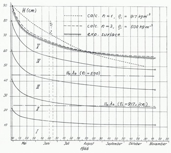
Fig. 4. Settling of sifted snow under its own weight at -10°C (inhomogeneous settling). Full lines indicate position of surface and internal points recorded with electrical level gauge. (IR Hr 26,1946), The dotted line indicates the calculated curve for n = 1 (Equation (4)), adjusted to experimental surface for t = 0 and 100 d. No agreement. The dashed line indicates the calculated curve for n = 3, w0 = 0.48 (θi = 500 kg m−3). Good agreement.

Fig. 5. Measured density profiles in a settling experiment (T = -2°C). Densification at the surface and with depth. (IR Nr 11, 1945).
Sometimes unexpected results were achieved as happened in …
Experiments on Snow Deformation
During 1945 to 1946, we looked for a yield-stress in deforming snow samples under low stresses. With this aim, hollow cylinders of snow were subjected to a torque. The distortion could be measured free of friction over a galvanometer mirror with high resolution. A yield-stress could not be established with certainty. However, when we removed the load from our cylinder, to our surprise, the twist started to turn back, as if moved by a ghost’s hand (Fig.6.). We identified this phenomenon as a visco-elastic after-effect. This effect was known for other materials and had been treated theoretically by Boltzmann, Wartenberg and others. An elementary model for this behaviour could be built up of linear viscous and elastic elements in a combined serial and parallel arrangement. (At this time the denomination as “Burgers-body” was not known to me).

Fig. 6. Visco-elastic after-effect. Twist of a hollow snow cylinder (arbitrary units) versus time under constant torque. Load removed after 31 min. (a) experimental curve (full line), (b) calculated curve for visco-elastic model (dashed line) with e representing elastic deformation. (IR tlr 24, 1946).
With two elastic parameters f1 and f3 being the constants of the springs in the model and with the viscous parameters n2 and n3, the deformation of the model could easily be described. For a first loading with constant stress (torque) α0, the strain (or twist) of the model is:

where the exponential term is the after-effect function, or P(t).
After removing the load, the elastic strain of the serial spring is immediately cancelled, and subsequently the strain the parallel elements is reversed according to the exponential after-effect function:

where t0 is the period with stress α0 and po = p(t0) (see Equation (5)), and t>t0.
In Figure 6, the behaviour of the model is represented by the dashed curves, whereas the measured deformation followed the full lines. Evidently the simulation was not perfect; the model was too simple. But we were quite happy and continued to work with the model and the cylinders.
For example, it was interesting to reverse the torque periodically and to look for the so-called Bauschinger effect. With the following set of equations the reaction of the model can be calculated:
ist reversal of stress (torque) after period t0 with stress |σ0| :


In the pertaining experiment the observed strain-rate under reversed stress was larger than calculated, which indicates a distinct desolidification.
Other work included increasing the load periodically by a constant amount Δ?0. We then went back stepwise to zero and did the same thing with reversed direction of torque. Again the theory produces the equations for the model:


The experiment followed the theory with some deviations. What we observed was a hysteresis in the strain-rate versus stress (Fig.7.).

Fig. 7. Twisting rate (arbitrary units) versus torque for a hollow cylinder of snow with stepwise increase, decrease and reversal of the torque over a full cycle (hysteresis). Full line represents model calculations, and circles represent experimental results. (IR Mr 24, 1946).
The visco-elastic after-effect should not be confused with stress relaxation after a sudden stop in the deformation rate. This was also calculated for the model :

After the experiments with snow cylinders, analogous tests were performed with polycrystal 1 in a ice and also translatory shear tests with snow. All samples showed a visco-elastic after-effect.
I must say that this strange behaviour, which could be tentatively explained by local stress accumulations in the granular structure of snow, was not very important in snow mechanics until recently. It was rather a nuisance. For treating dynamic processes, like the expansion of avalanche fractures, it has apparently gained some practical interest.
Now, let us look at a problem that was inspired by outdoor conditions. The photograph (Fig.8.) taken in April 1946 shows the so-called firn mirror or, after Seligman, the film crust. It results from complex energy-exchange processes at the snow surface and immediately below it. At this time the energy balance of the snow cover was of much interest to us, and we wanted to know, in particular, how variations of the snow-surface temperature penetrate the snow cover. This is among others a matter of ...

Fig. 8. “Firn mirror” on the snowfields south-east of Wei ssfluhjoch. On the plateau in the foreground is the experimental plot of the Snow Research Institute. (IR Nr 25, 1946).
Heat Conductivity of Snow
A number of empirical formulae were available for this, all related to snow density only. We had the impression that other parameters must also be involved and we tried to understand the mechanism of heat conductivity and to sort out contributions of the pores and, maybe, of other parameters besides density.
Was it a passion for playing with models, or was it presumption or just naivety that tempted me to simulate snow with a chain-model of spheres and to calculate its heat conductivity as the contribution of the ice structure? (IR Nr 25, 1946).
The model was built up of ice spheres connected to their neighbours with circular contact areas. Parameters were the radius of the spheres r and that of the contact areas p. Two methods for calculating the heat current through a sphere under a temperature difference 6T were envisaged. In one model (a), spheres with sliced off caps on either side were joined together, and a constant heat flux, spread evenly over every cross-section, was assumed. In the other model (b), the ice spheres were joined together with small spherical contacts and, from the analogy between an electrical field and a temperature field, the heat conductivity for a chain of spheres was calculated (see Ragnar Holm: Die Technische Physik Elektrischer Kontakte. Berlin, Springer-Verlag, 1941). In both models, r/p is the essential parameter, besides the heat conductivity of ice.
With these chains, looking like pearl chains, various simple structures were built up and their heat conductivities calculated. The result for an elementary cubic structure with a density of approximately 480 kg m−3 is presented in Figure 9(a). Assuming a ratio r/ ρ = 8, a heat conductivity of 10−3 cal cm−1 s−1 deg−1 is calculated with the electrical modelFootnote * . For another cubic structure (Fig.9.(b)) with only half of the spheres (thus with a density of 240 kg m−3),a heat conductivity of 0.25 × 10⁻³ units, i.e. a quarter of the other figure, comes out. With these examples the well-known quadratic relation between conductivity and density is supported. The heat conductivity of real snow was also measured with a spherical apparatus.

Fig. 9. Heat conductivity λ and density γ of structures built up of chains of ice spheres calculated for the electrical model (index i referring to ice).(a) spheres in an elementary cubic lattice,(b) chain structure containing half of the spheres of (a). (1 cal cm−1 s−1 deg−1 » 4.19?0−4 W m−1 deg−1)
If we plot the values calculated for the models as circles on a diagram of heat conductivity versus density, as it was available in 1946 (Fig.10.), the circles are found at about two-thirds of the measured conductivities, which seems reasonable since they represent the contribution of the ice structure only. Of course, this result is badly manipulated by the arbitrary grain boundary parameter r/p or, the other way round, we have demonstrated that there is such a parameter in the heat conductivity of snow as the grain boundary area.

Fig. 10. Heat conductivity of snow versus density. Curve (a): formula of J Devaux (1933). Curve (b): formula of M Jansson (1901). Curve (c): formula of H Abels (1892). Circles are calculated for chain models (ice structure only).
Other investigations of the period 1943-48 were concentrated on ...
Snow Metamorph ISM
The crystalline structure of snow was the favourite subject of Paul eke, Seligman and Bader. They had a clear conception of snow metamorphism, in particular on the formation of depth hoar. Their ideas induced us to look closer at the influence of temperature gradient and air circulation on this process.
An obvious and elementary experiment carried out in 1944, consisted of setting a cylinder of snow (55 cm long) under a strong temperature gradient for a period of a couple of weeks. The base of the snow cylinder was heated to -1°C, while the top was kept at the laboratory temperature of -10°C. For lateral insulation a layer of 15 cm of sawdust was used; the marvellous foam materials did not exist at this time. After 14 days the lower part of the sample was transformed into depth hoar, whereas in the upper section, where the gradient was much weaker (due to poor insulation) and the temperature lower, only little metamorphism was observed {Fig.11.). This first qualitative artificial gradient experiment demonstrated that the amount of the gradient and the gradient itself were important factors in metamorphi san. Gradient experiments have been repeated and refined many times since by others and by ourselves.

Fig. 11. Result of the temperature gradient experiment. Snow samples taken at indicated heights above heating plate. Depth-hoar formation decreasing with height. Marginal scale in mm. (IR Nr 4, 1944).
To investigate the influence of air circulation on snow metamorphism in natural snow cover, new snow specimens were sampled near the snow surface on days of snowfall from January to March 1946 and were immediately returned to their original locations in two different types of wrapping (Fig.12.). These were either air-tight tin boxes or plastic bags from which air could escape, but not enter, through a valve. A third sample consisted of the undisturbed snow at the same level. Conditions for snow pressure and air circulation were different in the natural undisturbed snow, in the boxes and in the bags: (i) in the snow cover, snow pressure corresponded to the overlying load and air circulation was free, (ii) in the bags, snow pressure was similar to that of natural snow, but air circulation from and to the sample was suppressed, except for sgueezed-out air, and (iii) in the boxes, snow pressure was relieved and air circulation was unrestricted, but there was no communication with neighbouring layers. Temperature conditions were probably similar for all parallel samples. On March 1946 all samples were dug out. Their characteristics are noted in Figure 12. Let us examine layer 3:

Fig. 12. Experiment on metamorphism and air circulation. New snow samples are locked in tin boxes (squares) and plastic bags (points) and relocated in the natural snow cover. Investigation of the content and comparison with natural samples in March 1946. Grain size (mm) and density (k m g−3) plotted on the right. (IR Nr 27, 1946).
In the natural layer, formation of depth hoar had advanced most, accompanied by the lowest decrease in density. In the bag, density had increased most and metamorphism was checked, and in the box an intermediate behaviour was observed for both features. Altogether, it became evident that free air and vapour circulation are important factors in snow metamorphism.
Structure Analysis
For identifying a snow structure in an objective manner guantitative methods are needed. Bader had introduced a sifting technique for measuring grain-size distribution, and he was probably the first to produce thin sections of snow for studying the coherent snow structure and measuring crystal fabrics.
We have adopted both techniques, but the sifting method was soon abandoned and replaced by a sedimentation procedure which is left aside here. The technique of thin-section preparation was not quite satisfactory either, for two reasons: Bader had filled the porous space of snow samples with the organic liquid tetrabromoethane which he solidified at temperatures below -10°C before cutting sections. Our objection to this substance was based primarily on its horrible, repulsive smell and its chemical aggressiveness. When I started working with it, it became evident to me that I would never be able to marry as long as I had anything to do with this liquid. Even participation at our communal lunch in the institute became a problem.
Looking for other substances with a melting point immediately below that of ice, I found aniline, but rejected it for the same reason. Ethyl laurate, tested already by Bader, was too soft and smeary, but was used for some time in spite of that. Finally, diethylphthalate appeared to be satisfactory in every respect. With this pore-filler another drawback of the former technique could also be eliminated: the light scattering of the filler. After cutting a section, the filler was liquefied by adding some tetraline, an organic solvent. From now on we were able to produce transparent thin sections without any nasty side-effects, and the door was open for all kinds of investigations on the structure of undisturbed snow. As an example, the analysis of depth-hoar fabrics on a horizontal field is pointed out. In a thin section from the horizontal field (Fig.13.(a)), chains of depth-hoar crystals (cups) oriented perpendicularly to the ground are observed. Figure 13(b) shows the corresponding orientation of tne c-axes, pointing preferentially in a vertical.

Fig. 13. Chain texture of depth hoar in a horizontal field (1948).(a) vertical thin section. Arrow (length 33 mm) pointing to the surface, (b) fabrics of crystal axes (projection on vertical plane). Preferred vertical orientation. direction. Thin sections of depth hoar on a slope were also analysed. The chains are still oriented in the direction of the temperature gradient, i.e. perpendicular to the slope, and the same holds for the crystal axes. In the meantime, preparation and analysis of thin sections has been refined by Jaccard, Good and many others. Perla has recently presented an excellent account in the Journal of Glaciolagy.
For me, the change from tetrabromoethane to diethylphthalate had another important effect: the ban was broken, Rita entered my life and gave it a new dimension.
We have looked at a number of old attempts, at things that were started, and many of them were dropped again without visible reason. This was the first occasion to open the box for an hour, and now it may be closed again.


