


1. Introduction
Austfonna (79–80° N, 20–27° E), an ice cap on Nordaustlandet, Svalbard, has an area of 8120 km2, a maximum altitude of 783 m and a maximum ice thickness of about 560 m (Reference Dowdeswell, Drewry, Cooper, Gorman, Liestøl and OrheimDowdeswell and others, 1986) (Fig. 1). The ice cap is divided into a number of drainage basins which appear to be characterized by diverse flow regimes (Reference DowdeswellDowdeswell, 1986). Svalbard is at the northern extremity of the warm North Atlantic drift. As a result, the archipelago is particularly sensitive to climate shifts associated with changes in the North Atlantic drift.
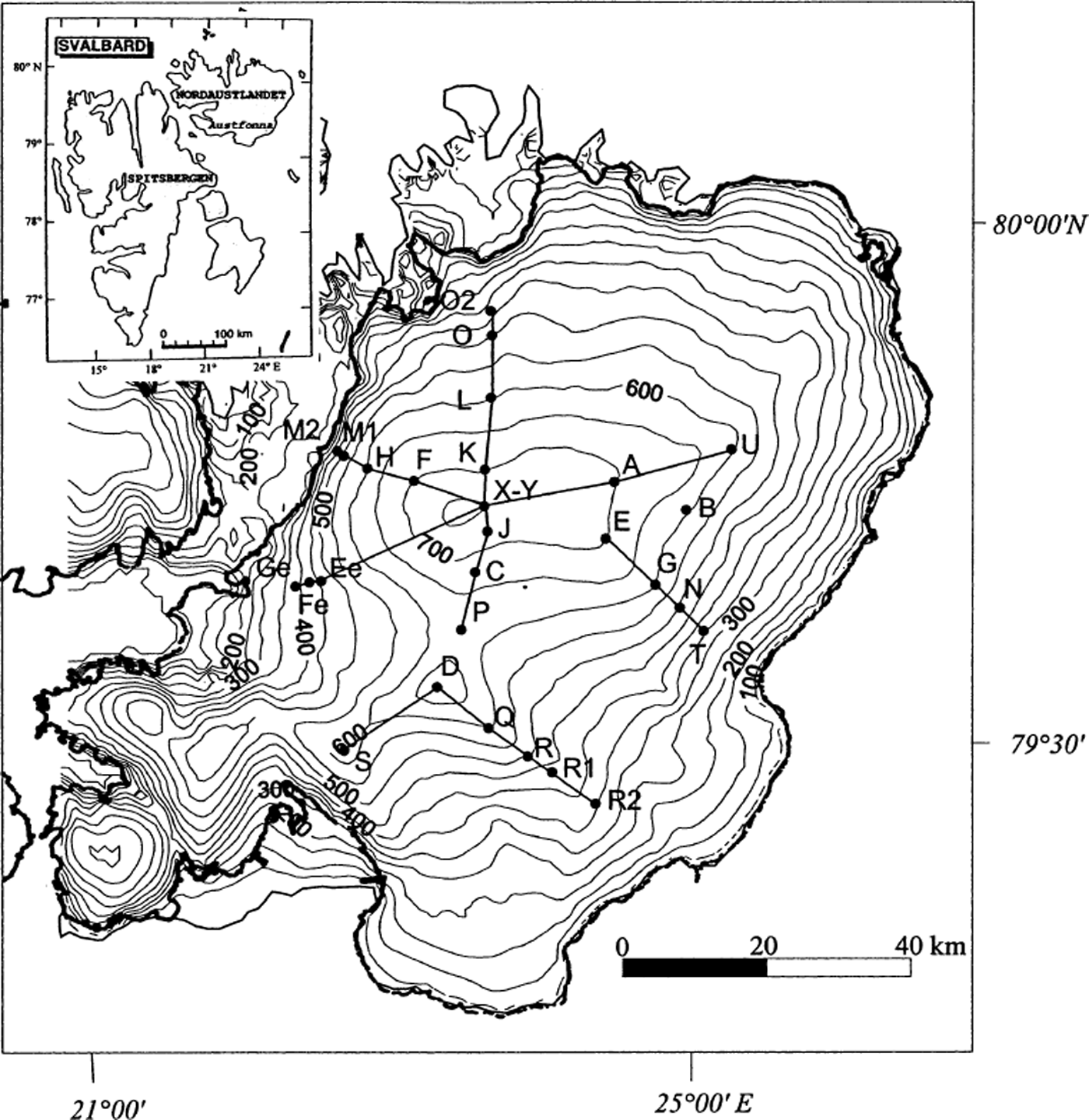
Fig. 1. Map of Austfonna, with location of the drilling sites, GPR transects and ice-cap contour and an inset showing the location of Nordaustlandet within Svalbard.
A number of glaciological investigations have been conducted on Austfonna. Traverses across the ice cap were carried out by A. E. Nordenskjold in 1873, the Oxford expedition in 1924 (Reference BinneyBinney, 1925), H.W:son Alhmann in 1931 (Reference AhlmannAhlmann, 1933),V. Schytt in 1957 and 1958 (Reference SchyttSchytt, 1964) and J. A. Dowdeswell in 1983, 1986 and 1987 (Reference Dowdeswell and DrewryDowdeswell and Drewry, 1989). Deep ice cores were obtained by Soviet teams at Vestfonna in 1981 and Austfonna in 1985 and 1987 (Reference Punning, Martma, Tyugu, Vaykmyae, Pourchet and PinglotPunning and others, 1986; Reference Zagorodnov and ArkhipovZagorodnov and Arkhipov, 1990) and by Japanese scientists (National Institute of Polar Research (NIPR)) at Vestfonna in 1995 and Austfonna in 1998 and 1999 (Reference Watanabe, Kamiyama, Kameda, Takahashi and IsakssonWatanabe and others, 2000).
Data on snow-accumulation distribution are a prerequisite to sensitivity modelling of ice caps by means of energy-balance models (Reference Fleming, Dowdeswell and OerlemansFleming and others, 1997). Little is known of the present mass balance of Austfonna, and field investigations were necessary to obtain data on snow accumulation and the net accumulation pattern. This paper presents results of these recent field investigations on Austfonna. The aim of this work is to determine (a) the 1997/98 and 1998/99 winter accumulations and mean annual net mass-balance patterns over the ice cap, (b) the mean equilibrium-line altitude (ELA), (c) the mass budget of the Austfonna accumulation area and (d) natural and artificial radioactive deposition over the Austfonna accumulation area.
2. Data Sources and Methods
2.1. Ice-core data
During two field seasons on Austfonna in April 1998 and April–May 1999, eight and twenty-one shallow ice cores, respectively, were drilled in the accumulation area and in the upper part of the ablation area of Austfonna (Fig. 1; Table 1) (Reference Melvold, Hagen, Eiken and PinglotMelvold and others, 1999). The cores were retrieved with a Polar Ice Coring Office (PICO) lightweight auger for shallow depths down to about 15 m. The drill produced cores with a 77 mm diameter and a mean length of about 40 cm. In addition, two deeper ice cores were drilled in 1998 and 1999 by the NIPR (K. Kamiyama and others, unpublished information). These cores were drilled with an electromechanical drill down to 118 and 288 m, respectively.
Table 1. Ice-core locations at Austfonna in 1998 and1999 with mean density of winter snow, accumulation during the 1997/98 and 1998/99 winters, and 210Pb winter deposition over Austfonna
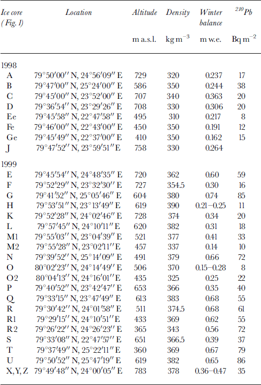
The snow and firn densities were determined immediately after the retrieval of the ice cores by measuring the diameter, length and weight of each core section. Figure 2 shows density profiles along cores X, E, G, N and T. While the density increases semi-continuously for cores X and E, it increases abruptly at depths of about 2 m, under the winter snow layer for ice cores G, N and T. The density of the 1998/99 winter snow cover was found by averaging the density of the upper core sections of all ice cores (Table 1). These densities along each transect were used to convert snow-depth measurements from snow-probing and ground-penetrating radar (GPR) measurements to m w.e. depth.
Fig. 2. Snow-ice density and 137Cs (from Chernobyl) profiles with depth for the southeast (XEGNT) transect (Fig. 1). Note the changing scale for 137Cs.
Four snow pits, close to cores X, Y and Z (Fig. 1; Table 1), were studied in April 1999 (personal communication from L. Karlof, 2000). The most important details in the stratigraphy were the existence of ice layers (2–5 cm thick) at 1.1–1.4 m depth. In a given pit, there are several thin firn or ice layers under the first ice layer. It was evident that the layer at about 1.25 m represented the late-summer surface of 1998 and that the thin firn and ice layers belonged to earlier periods during the same summer season, associated with surface melting, and followed by percolation some distance into the snow-pack before the water refroze and caused the formation of ice layers. This shows that all the snow above this depth was accumulated during winter. Similar multiple layers were also found in the firn cores. Superimposed ice with a density of 900 kg m−3 was found just below the winter snow layer for ice cores G, H, L, M1, O, N, R, R1, R2, T and U (Fig. 1).
Snow temperatures were measured with a thermistor string at core sites A, C, K and E. Despite clearly negative temperatures at 10 m depth, the temperature gradient indicates that the ice is close to the pressure-melting point at about 20 m. At greater depths, colder ice (about −8°C at 160 m depth) was found in a deep ice core drilled on the ice cap (Reference Zagorodnov and ArkhipovZagorodnov and Arkhipov, 1990). This confirms Schytt’s (Reference Schytt1964, Reference Schytt1969) proposal that the Austfonna ice cap has a subpolar thermal regime characterized by an inner core of temperate ice surrounded by an annulus of cold ice.
2.2. Core handling and laboratory analyses
Nuclear weapons tests in the 1950s, 1960s and 1970s, and the Chernobyl accident in 1986, emitted large amounts of man-made radioisotopes (e.g. 134Cs and 137Cs) into the atmosphere. Some of this material reached glaciers in the Arctic, providing permanent records of deposition. In 1999, the Chernobyl layer in the Austfonna ice cap was never deeper than 9 m, so it was possible to determine the mean annual net mass balance for 12 years over the whole Austfonna accumulation area by retrieving a series of shallow ice cores. In the present study, we identify both natural and artificial radioactive signatures in shallow ice cores drilled in Austfonna in spring 1998 and 1999. We determined the mean snow accumulation from the radioactive layers associated with Chernobyl and the atmospheric nuclear tests layer, the latter having a maximum in 1963 in the Arctic. In addition, GPR methods have been used to derive continuous profiles of the 1998/99 winter snow cover from seven profiles.
After the fieldwork, all the cores were subsampled (cut into sections approximately 15–20 cm long) in cold rooms in order to conduct high-resolution gamma spectrometry. The radiochemical preparation of these samples mainly involved melting, acidification and filtration, and final standardized mounting for gamma radioactivity as described by Reference Delmas and PourchetDelmas and Pourchet (1977). Altogether, the 1999 cores consist of 700 samples for a total length of 175 m, whereas in 1998 we prepared 250 samples for a total length of 90 m. The Japanese deep ice cores were subsampled by the NIPR and the Norwegian Polar Institute (NPI) between the surface and 40 m depth for radioactivity and other measurements (K. Kamiyama and others, unpublished information).
The high-resolution gamma spectrometry analyses were conducted in a specially designed laboratory at the Laboratoire de Glaciologie et Géophysique de l’Environnement, Grenoble (Reference Pinglot and PourchetPinglot and Pourchet, 1994). It was possible to determine both natural and artificial radioactivity in the snowpack. The stratigraphy of the radioactive layers includes 137Cs from the nuclear tests (1954–74) and Chernobyl (1986), as well as 210Pb of natural atmospheric origin (Reference PinglotPinglot and others, 1994). In order to determine the 210Pb winter deposition, gamma spectrometry was conducted on the upper samples of the cores representing the winter 1997/98 and 1998/99 snow accumulations.
2.3. GPR and GPS survey: error analysis and data processing
During the fieldwork in 1999, we used a RAMAC impulse GPR system operating at 500 MHz and two Ashtech Z-XII global positioning system (GPS) receivers to profile Austfonna. Snow radar and GPS data were collected continuously along 300 km long traverses following the routes between the core sites (Fig. 1). The dataset comprises approximately 150 000 GPR traces and 22 000 GPS points. Manual snow-depth measurements were taken at the core sites and at a number of intermediate points along the transects. These 50 manually observed snow depths were used to check and calibrate the snow depth obtained by the GPR.
The radar control unit, laptop computer, GPS antenna and receiver were operated from a sledge pulled by a snowmobile. The radar antenna was mounted on a non-metallic sledge pulled 2 m behind the first sledge with the GPS and GPR units. Each 500 MHz GPR record was collected in the form of 512 samples with a sampling frequency of 4865 MHz, giving a time window of 105 ns for each trace. Eight individual radar returns were stacked to increase the signal-to-noise ratio. This stacked trace was recorded in the laptop computer. To determine locations, differential or kinematic GPS was used. In addition to the on-board GPS receiver (rover), one stationary receiver was located at the camp site. This reference receiver was related to a fixed geodetic point beyond the ice cap. The method is fully described by Reference Eiken, Hagen and MelvoldEiken and others (1997).
GPR and GPS data were sampled with fixed time intervals of 0.5 and 5 s, respectively. The spatial measurement interval therefore depends on snowmobile speed (∼4 m s−1), and averaged around 2 and 20 m for GPR and GPS, respectively.
2.3.1. GPR processing
The radar receives signals from different reflectors in the snowpack. In order to obtain quantitative snow-accumulation measurements from GPR data, it is necessary to convert time-dependent radar return signals to depths. The winter 1998/99 snow–ice or snow–firn interface must be identified and separated from the other reflectors. A time-varying gain function was used to amplify the signal at depth. Usually two dominant signals can be observed (Fig. 3): the reflection returned from the surface of the snow cover, which serves as the time reference; and the echo from the snow–firn or snow–ice interface. In the ablation and superimposed-ice area, the snow–ice reflector can easily be identified using the layer reflection intensity since the winter snow cover lies on top of uniform cold ice. In the accumulation area, the snow–firn interface is less distinct, due to a less homogeneous and less well-developed summer surface. The snow cover lies on top of heterogeneous firn (firn, superimposed-ice and ice layers), as shown in the pit and ice-core stratigraphy (Fig. 2) . The winter 1998/99 snow cover was identified using the layer reflection intensity correlated to the core stratigraphy and manual probing.

Fig 3. GPR signals: typical section of a 500 MHz record from the south transect DQRR1R2 around core R (Fig 1), which shows a clear reflection from the ices–now interface. The distance between the traces is approximately 2 m, and a TWT of 10 ns gives a depth of about 1.15 m in snow. Repeated events (e.g vertical ellipses) are system ringing.
To construct a snow-distribution map from these GPR data, the onset time of the surface and snow–ice/snow–firn reflections must be determined. An interactive mouse-driven computer program (SIRDAS Data Analysis System from SUSAR Consulting AS) was used to determine the onset times and the two-way-travel times (TWT) between the snow surface and snow–firn/snow–ice interface along most of the GPR profiles (80%). Gaps occurred in the output of the automatic digitizing when the signal from the snow–firn interface was too weak to be determined. In those areas, no accumulation data were obtained from the GPR measurements.
The electromagnetic wave speed (v s) through snow and firn can be determined by
where c 0 (2.988 × 10⁸ m s−1) is the speed of the electromagnetic wave in a vacuum and ε is the dielectric constant. The dielectric constant, in turn, is a function of several parameters, of which the most important are density and water content (Reference Ulaby, Moore and FungUlaby and others, 1986; Reference Kovacs, Gow and MoreyKovacs and others, 1995). Dry snow and firn are assumed everywhere in spring, and the thermistor data from the core sites show subfreezing temperatures in the upper 10 m of the snow/firn pack. Density will thus be the most important factor determining the wave propagation speed. The snow densities measured at the core sites varied from 340 to 390 kg m−3 , averaging to 375 kg m−3. Based on empirical models for estimation of the dielectric constant, this should give a dielectric constant close to 1.7, as also used by Reference Winther, Bruland, Sand, Killingtveit and MarechalWinther and others (1998) investigating snow distribution on Spitsbergen, Svalbard. The snow thickness was calculated from the TWT using an average electromag netic wave velocity in snow of 230 m μs−1, following from using ε = 1.7. A constant wave speed was assumed to simplify the depth calculations. Along the GPR profiles, the snow thicknesses were translated into snow accumulation in m w.e. using the measured depth–density distributions.
2.3.2. GPR error analysis and data treatment
The accuracy of the accumulation thus obtained, in m w.e., depends on the accuracy of the wave propagation speed, snow density and interpretation of the radar recordings.
The error introduced by density variations was assessed. The wave propagation speed was estimated using maximum (390 kg m−3) and minimum (340 kg m−3) densities. The difference in the wave speed between these two cases gave a 4% difference in the estimated snow depth. The effect on the calculated accumulation could be up to 10% in the measured depth range (0.5–3 m).
The automatic digitizer can pick up the onset times from the snow surface to within half the sampling interval, that is equal to about 0.23 m of snow (Fig. 3). The quality of the reflection from the snow–ice/snow–firn interface, however, is influenced by several factors:
(1) the thickness of the snow cover and the spreading loss,
(2) the roughness of the interface,
(3) interference from nearby reflections rather than a direct representation of the individual discontinuities in impedance themselves (especially in the accumulation area), and
(4) the dielectric constant contrast between the snow and ice or firn below the snow mainly through changes in density (Refzlaff and others, 1993; Reference Rosenberger, Oerter and MillerRosenberger and others, 1997).
All these factors affect the accuracy of the automatic depth determination.
Moreover, if the wavelengths used are greater than the thickness of the individual ice layer/snow layers, each internal horizon corresponds to interference from several layers (Reference HarrisonHarrison, 1973). Interference could lead to random vertical displacement of some horizons and the visual impression of a high-resolution record. On Austfonna, the pit and core studies show several thin, closely spaced ice–firn layers just below the summer surface. We could thus expect interference in our GPR data which will affect the determination of the onset time for the snow–firn interface and lead to noise in the derived TWT.
The estimated snow accumulation shows large spatial variations over short distances (50–100 m) (Fig. 4a and b). We estimated the variability along transects for spatial averages of groups of data. The variability is given as a coefficient of variation expressed by the ratio of the standard deviation of a given number of accumulation values (25 points/500 m) to the mean value. The variability for the different groups of data along transects ranges from roughly 25% for the groups of data derived from the accumulation area to about 12% for data from the ablation area. The higher noise signal found in the accumulation area is probably a result of the random vertical displacement of the GPR horizon due to interference of the radar signal and to less homogeneous GPR horizons. By spatially averaging our GPR data we obtained data with low variability, reflecting primarily real spatial differences in the snow-accumulation pattern. All accumulation data were therefore spatially averaged using a 25-point moving average. Analysis of several digitized records indicates an average digitizing error of 5 cm for the snow–ice reflection and 15 cm for the snow–firn reflection.
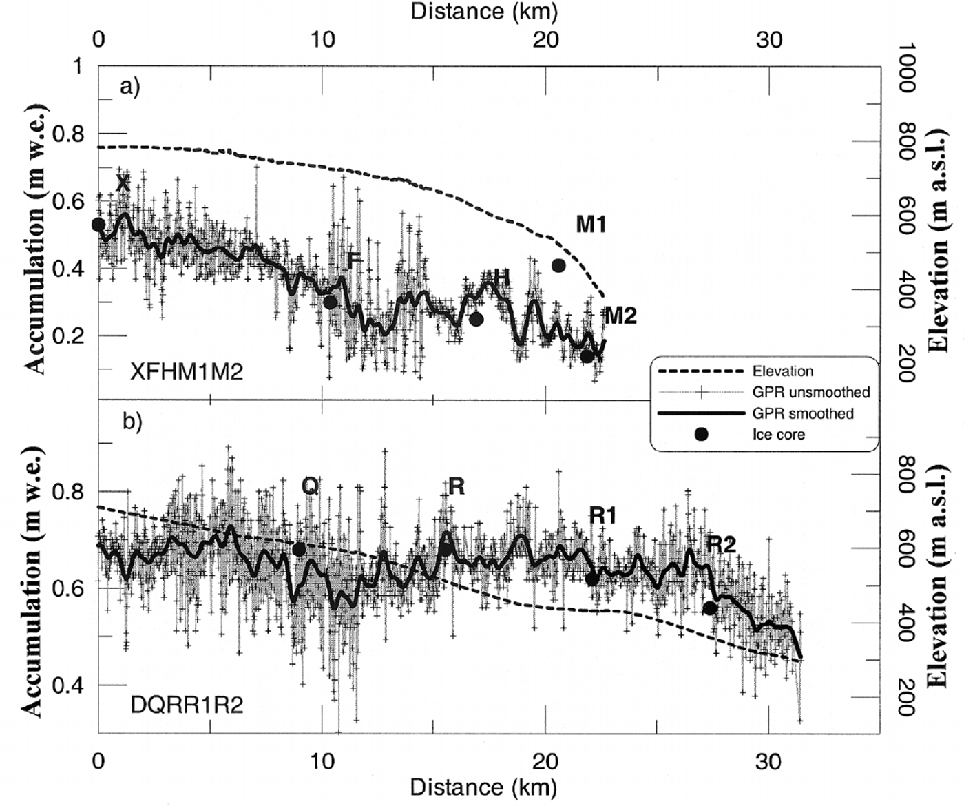
Fig. 4. Snow depth (m w.e.) and surface elevation (dotted line) for northwest (XFHM1M2) and south (DQRR1R2) transects (located in Fig 1), measured by radar and GPS. Both unsmoothed and smoothed (thick black line) radar data are shown. Snow depths (m w.e.) for the core sites along the transects are also shown (black circles).
2.3.3. Differential GPSfor positioning
Ashtech’s Precise NAVigation (PNAV) software was used for processing the GPS data. The PNAV software produces the so-called “on-the-fly” (OTF) ambiguity resolution in the measured GPS code and phase data. For OTF initialization, the first few measurements are used to resolve the phase ambiguities, which means determining the integer number of wavelengths between the satellite and the receivers. After this, a Kalman filter is used to calculate both static and kinematic positions. The position of the rover antennae relative to the fixed GPS receivers is then determined along each transect. Static fixed solutions were determined for the beginning and the end of the survey and beside core sites and all points where the snowmobile stopped. The GPS-measured heights are related to sea level by subtracting a constant geoid height of 26.62 m from the World Geodetic System 1984 (WGS84) derived ellipsoidal heights.
2.3.4. Geo-coding
The horizontal and vertical position of the GPR traverses could be determined from the kinematic GPS survey. However, a major obstacle to obtaining an accurate horizontal and vertical position of each GPR data point is the relatively poor density of the GPS measurements. GPS data were obtained at 5 s intervals, and GPR at 0.5 s intervals. The starting and ending coordinates of the individual GPR transect were measured. The horizontal position of the GPR traces is determined by interpolation, assuming constant velocity and thus equidistant sampling space between the starting and ending coordinates for each GPR file. The elevation is determined by linear interpolation between the closest pair of GPS coordinates for each shot. As a result, locations (x, y, z) were determined to within 0.5 m both vertically and horizontally for most of the data points.
GPS data were also used to fix the position of core sites and current geometry of the surface, resulting in accuracies of about 1 m vertically and 5 m horizontally (Table 1).
3. Results
3.1. Radioactivity
3.1.1. 210Pb winter deposition
The measured 210Pb (natural isotope) winter deposition shows large annual and interannual variations (Table 1). The mean 210Pb fallout varies by a factor of 2 between winter 1997/98 (18.6 Bq m−2) and 1998/99 (43.7 Bq m−2), with standard deviations of 9.6 and 26.5 Bq m−2, respectively. From Figure 5 it is evident that there is a clear positive correlation (r 2 = 0.88) between 1998/99 winter snow-accumulation rate and 210Pb fallout, with high accumulation rates giving high Pb depositions. Interannual 210Pb winter deposition variation can thus be ascribed to differences in accumulation and not to differences in deposition processes.
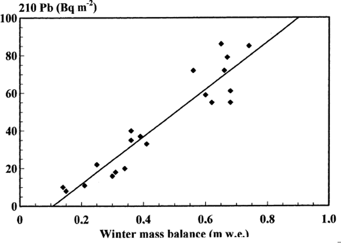
Fig. 5. 210Pb fallout vs 1998/99 winter mass balance.
3.1.2. Reference and ablation layers
The Chernobyl layer has been identified in 19 ice cores from the accumulation area (Table 2). The Chernobyl deposition varies from 1 Bq m−2 (at core sitej) up to 47 Bq m−2 (at core site X), with all activities corrected to 1 January 2000. The mean value for 19 determinations is 10 Bq m−2, with a 10 Bq m−2 standard deviation. There is no clear relationship with altitude, and a strong spatial variability was observed. For instance, 137Cs depositions of 5 and 47 Bq m−2 were measured for ice cores X and Z which are situated only a few hundred metres apart.
Table 2. Detection of the Chernobyl layer in the 1998 and1999 Austfonna ice cores: real and w.e. depths, 137Cs deposition (on 1 January 2000), winter mass balance and MANMB (min. and max. values, for the time period from 1986 to the date of drilling)

Figure 2 shows density and 137Cs profiles for ice cores X, E, G, N and T along the southeast transect (Fig. 1). The peak in 137Cs corresponding to the Chernobyl layer is clearly seen in one sample (15–30 cm long) along each core. The depth ranges in Table 2 correspond to the length of the sample. As the altitude decreases from ice core X (783 m) to ice core N (491 m), the Chernobyl layer depth decreases from 8.9 m to 4.47 m.
The concentration of 137Cs in core T is an order of magnitude larger than in the other cores along the transect. Similar high 137Cs concentrations are present in cores Fe, Ge, Ee, M2 and O2 (Table 3). In all these cores, the high 137Cs concentration was found just below the winter 1997/98 and 1998/99 snow covers. In ice core T the 137Cs concentration is as high as 1353 m Bq kg−1 and the deposition is 119 Bq m−2 (Fig. 2). This concentration is much higher than that found in the 19 cores where the Chernobyl layer is present (cf. 137Cs values in Tables 2 and 3). High concentrations of 137Cs and 210Pb have also been found in ice cores drilled on Kongsvegen (Reference Lefauconnier, Hagen, Pinglot and PourchetLefauconnier and others, 1994) and Finster-walderbreen, Spitsbergen (Reference Pinglot, Pourchet, Lefauconnier and CreseveurPinglot and others, 1997). These authors attributed this to the drilling of these cores in the ablation area, where all artificial radioactive deposits are concentrated, giving rise to high measured values. The dust layer formed at the surface in the ablation area acts as a filter that traps radioactive materials that have been removed from the basin. High concentrations thus indicate that the cores are drilled in the ablation area. In Figure 6, the respective concentrations of 137Cs and 210Pb isotopes are plotted for cores Fe, Ge, Ee, M2, O2 and T. There is a strong positive correlation between the two isotopes. This suggests that the concentration process of radioactive materials is the same for both artificial and natural radioactivity. This is in accordance with previous work on other Svalbard glaciers (Reference Pinglot, Pourchet, Lefauconnier and CreseveurPinglot and others, 1997).
Table 3. 137Cs and 210Pb deposition of the dust layers
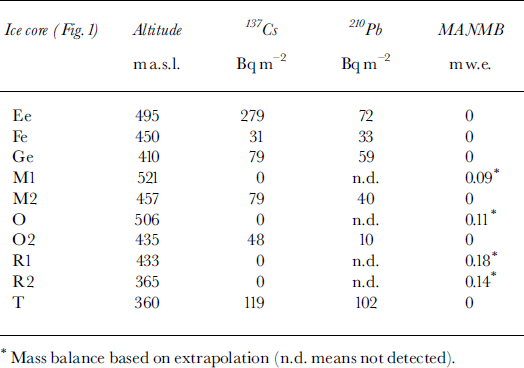

Fig. 6. 210Pb vs 137Cs deposition for cores Ee, Fe, Ge, M2, O2 and T (located in Fig. 1).
In cores M1, O, R1 and R2, only negligible amounts of Pb and Cs fallout were found. Based on their positions, we propose that the cores are from the accumulation area (Table 3), but, since melting and percolation are quite intense, the deposited particles may have been washed out of the snowpack or transported to greater depths. The mean annual accumulation at these locations could only be deduced by extrapolation from the mean annual net mass-balance gradients.
In core J we found two peaks in the 137Cs radioactivity profile: one at an original deposition depth of 8.82 m, extending down to 10.47 m (Table 2), and the second at a depth of 22.53–22.88 m. These peaks correspond to deposition from the Chernobyl accident in 1986 and the nuclear tests (1954–74) which led to a radioactivity peak in 1963.
3.2. Winter accumulation
Results from the radar soundings together with surface elevations and snow accumulation (winter mass balance) at ice-core locations along the northwest transect are presented in Figure 4a (XFHM1M2 (22 km) in Fig. 1). GPR sounding data yield additional information on winter snow-accumulation distribution between the core sites. The GPR data were tuned to the depth of the previous summer surface. The accumulation from pit studies shows substantial variability over short distances. This presumably reflects real spatial variability owing to wind scouring and redeposition, and indicates that individual measurements are not a reliable estimator of the average accumulation rates. Figure 4 shows the limited representativeness of the manual snow-accumulation measurements. It shows that there are marked spatial variations in accumulation rates over both short and long distances along the transects. The smoothed snow accumulation (Fig. 4a) ranges from 0.14 to 0.56 m w.e., with a 0.35 m w.e. mean value. There is a clear correlation between elevation and snow depth, with values ranging from <0.20 m w.e. at about 375 m a.s.l. to >0.60 m w.e. at 780 m a.s.l.
Data are also shown for the south transect (Fig. 4b, DQRR1R2 in Fig. 1). As with the other profile, there is a relationship between elevation and snow depth ranging from 0.46 m w.e. at 300 m a.s.l. to 0.69 m w.e. at 600 m a.s.l.. Between 0 and 20 km, there is a decrease in the snow accumulation with increasing elevation. The smoothed snow accumulation ranges from 0.50 to 0.73 m w.e., with a 0.64 m w.e. mean value. The amount of accumulation along the south transect is about 0.30 m higher than for the northwest transect. The accumulation as a function of elevation varies between the two transects, ∼0.09 m per 100 m and ∼0.03 m per 100 m, respectively. These two profiles are situated northwest and southeast of the main ice divide (Fig. 1). Similar changes in snow-accumulation gradient could also be seen from the eastern to the western part of the main ice divide, with highest accumulation in the east.
These data have therefore been used to construct the map of the winter accumulation for 1998/99 as shown in Figure 7. The accuracy of the map is quite high along the transects, and decreases rapidly with increasing distance from them. It shows the overall snow-accumulation pattern on the ice cap, including the main trends, with decreasing values from east to west and from south to north. The 1998/99 winter accumulation decreases from 0.65 m w.e. in the southeastern areas down to about half this value in the northwestern areas.
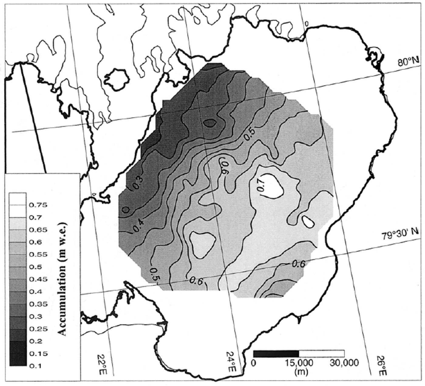
Fig 7. Distribution map of the 1998/99 winter mass balance (m w.e.) on Austfonna, based on ice cores and GPR measurements.
Based on the snow distribution in Figure 7, the winter accumulation on Austfonna was calculated to be 2.69 × 10⁶ m3, on the 5474 km2 investigated area of the ice cap, corresponding to an average 0.49 m w.e. of snow accumulation.
Table 1 shows winter accumulation for winters 1997/98 and 1998/99 found at the core sites, with values (based on 8 and 20 measurements made on a large part of the ice cap) of 0.25 ± 0.06 and 0.45 ±0.02 m w.e., respectively. Similar differences were found by Reference SchyttSchytt (1964), with a total accumulation for 1957/58 that was 50% higher than for 1956/57.
3.3. Mean annual net mass balance
The mean annual net mass balance (MANMB) for the period from 1986 to the date of the core retrieval has been determined for the 19 cores where the Chernobyl reference layer is preserved. After translation to m w.e. and divided by the time-span between core retrieval and the datum stratum, and with subtraction of the winter 1997/98 and 1998/99 snow layers, the MANMBs were determined over 12 or 13 years (137Cs fallout from 1986 to 1998 or 1999). The measured net mass balance ranges from 0.19 to 0.54 m w.e. a−1 (Table 2), and the variations mainly depend on the altitude (Fig. 8). The MANMB is not constant for a given altitude, however. For instance, it is 0.34 and 0.54 m w.e. at ice cores D (708 m a.s.l.) and C (707 m a.s.l.), respectively. The MANMB exhibits maximum values (0.53–0.55 mw.e.) close to the top of the ice cap (Fig. 9). A 0.05 m w.e. MANMB was determined at Isdomen (79°33′ N, 25°05′ E; 374 m a.s.l.) (Reference Dowdeswell and DrewryDowdeswell and Drewry, 1989). This is in accordance with our results.
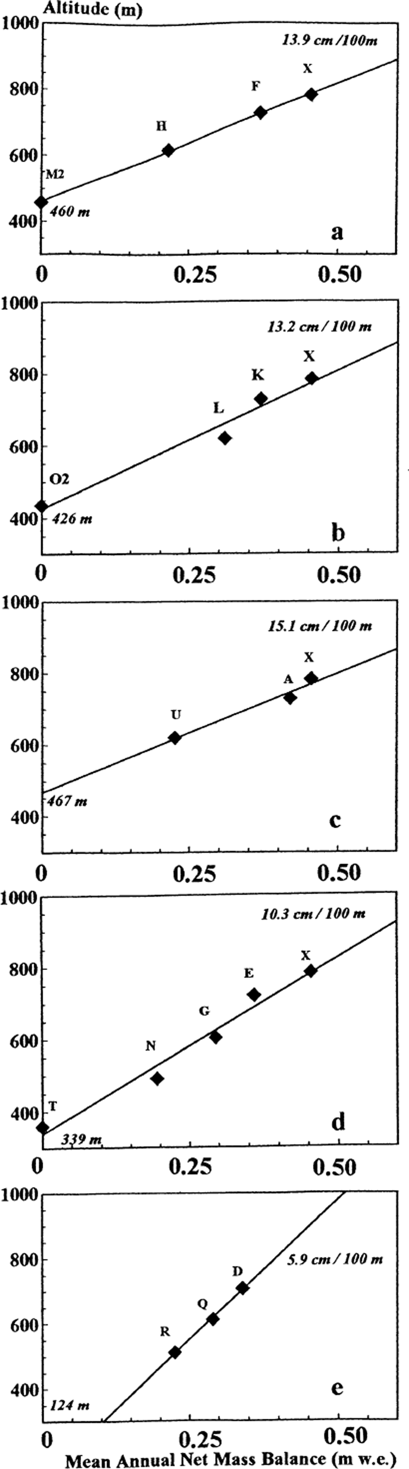
Fig. 8. Relationship between MANMB at the core sites and altitude (Fig. 1), for five different transects: (a) northwest (XFHM1M2); (b) north (XKL002); (c) east (XAU); (d) southeast (XEGNT); (e) south (DQRR1R2). The altitudinal gradients (cm w.e. per 100 m) and the ELAs (m) are noted in italic for each transect.
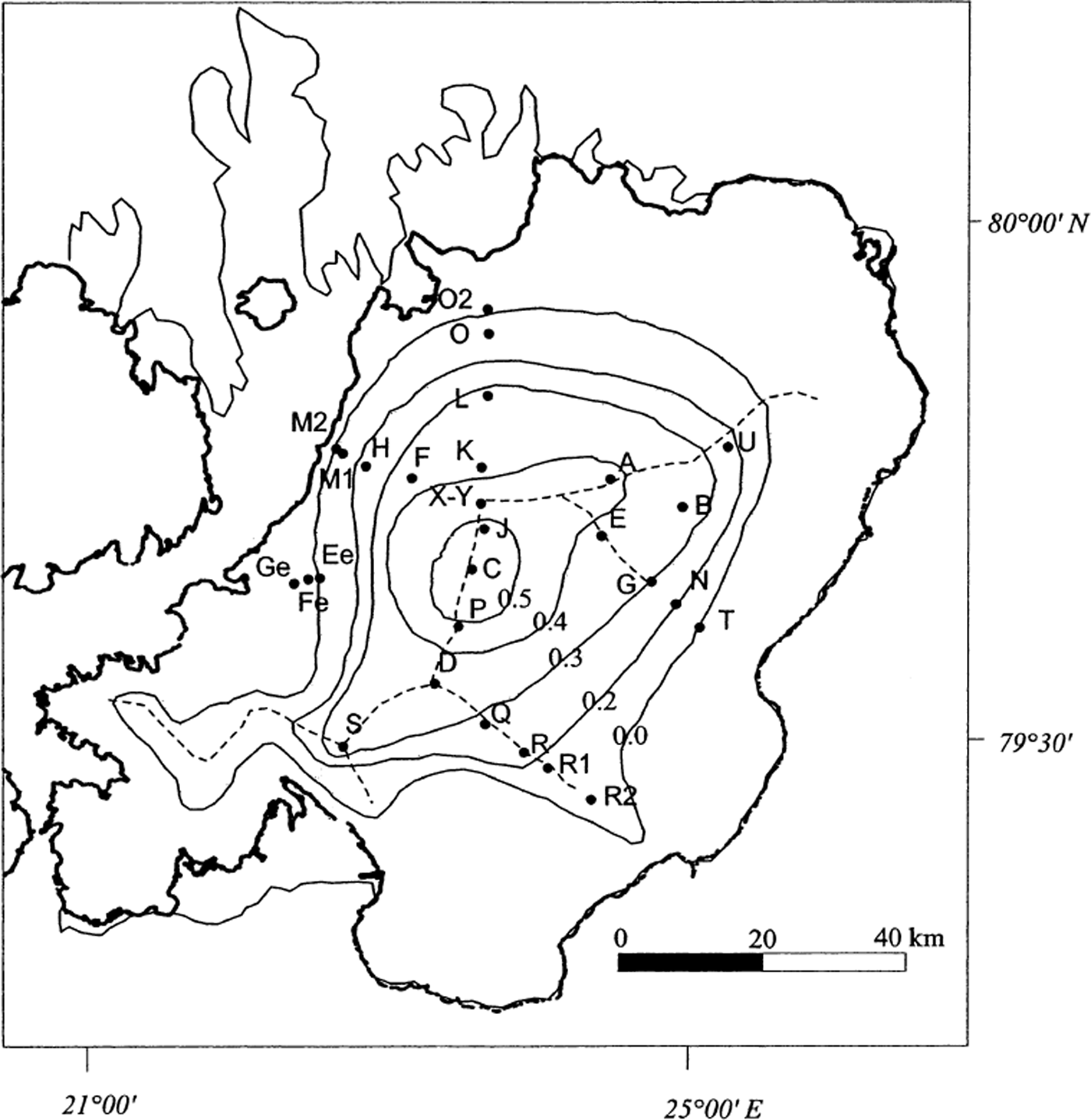
Fig. 9. Distribution map of the MANMB (m w.e.) on Austfonna. Isopleths correspond to MANMB contours: 0.5, 0.4, 0.3, 0.2 and 0.0 m w.e. a−1. Dashed lines represent the main ice divides.
The MANMB values are higher than the 1997/98 winter mass balances (Table 3). This is also true for eight ice cores retrieved in 1999 compared to the 1998/99 winter mass balances. This demonstrates that these winter 1998/99 mass balances have lower values than the mean value over the last 12–13 years.
The mean equilibrium-line altitudes (ELAs) are determined for five transects, fitting the observations to a linear altitudinal gradient of the MANMB (Fig. 8a–e). From these gradients the MANMB could be estimated for cores M1, O, R1 and R2 (Table 3). The northwest transect (XFHM1M2) indicates an ELA at 472 m a.s.l. and a mean snow-accumulation gradient of 0.15 m w.e. per 100 m. The southeast (XEGNT) and south (DQRR1R2) transects show quite different values. For the southeast transect, the ELA is as low as 339 m a.s.l. and the gradient is 0.10 m w.e. per 100 m. This is in agreement with the thicker winter snow layer deposited in this area. These determinations are also in close agreement with earlier investigations. Reference SchyttSchytt (1964) indicated 450 and 300 m a.s.l. ELAs for west Vestfonna and northeast Austfonna, respectively; Reference Dowdeswell and DrewryDowdeswell and Drewry (1989) determined an ELA at 330–400 m a.s.l. for northeast Austfonna. The south transect shows a gradient of 0.06 mw.e. per 100 m, along with a surprisingly low ELA at 124 m a.s.l. that gives a very large accumulation–area ratio (AAR). This determination for Bråsvellbreen may explain the surge character in this part of Austfonna (largest surge in Svalbard in 1937). From the determination of the ELAs, the AAR is 0.45. These ELAs and gradients found at Austfonna can be compared to values for other Svalbard glaciers. The ELA in 1980 at nearby Storoya was about 115 m a.s.l. (Reference JonssonJonsson, 1982). Kongsvegen and Kronebreen in northwest Spitsbergen have higher ELAs at 500 and 650 m a.s.l., respectively, and much higher net mass-balance gradients of 0.33 and 0.32 m w.e. per 100 m, respectively. The difference is due to a more maritime climate on the west coast of Spitsbergen than on Nordaustlandet.
A map of the MANMB in the accumulation area was formed based on the 19 ice cores in the accumulation area, the ELA variations and the location of six cores (Ee, Fe, Ge, M2, O2 and T) in the ablation area (Fig. 9). The larger accumulation areas are located to the east and south of the ice divide (Reference Dowdeswell and CooperDowdeswell and Cooper, 1986). The map allows us to calculate the mean annual net mass budget of the Austfonna accumulation area (Table 4).
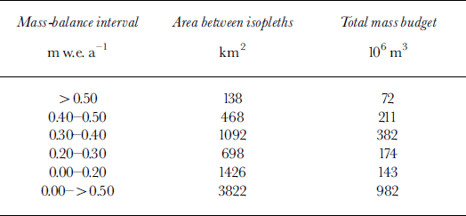
Table 4. Distribution of the area and total mass budget for the different mean annual net mass-balance isopleths on Austfonna (Fig. 9)
Based on the two peaks in Cs radioactivity found in the 1998 Japanese deep core, it was possible to estimate the MANMB for two separate periods, 1963–86 and 1986–97: 0.50 and 0.52 m w.e., respectively. This difference is not significant. The temporal variation of the MANMB has previously been studied from ice cores over Svalbard, using the same dating horizons. MANMB at these locations does not indicate any significant change on Svalbard either (Reference PinglotPinglot and others, 1999).
4. Discussion
4.1. 137Cs and 210Pb depositions
A number of studies have been carried out on glaciers in Svalbard to determine the 137Cs deposition in the Chernobyl layer (Reference PinglotPinglot and others, 1994). In general, the deposition on Austfonna varies widely, from only a few Bq m−2 up to 47 Bq m−2, with a mean of 10 Bq m−2 (19 cores in the accumulation area) (Fig. 9). Larger variations are also found for cores drilled only a few hundred metres apart (e.g. Austfonna cores X and Z, respectively 5 and 47 Bq m−2). These variations must be due to different amounts of fallout or post-depositional processes.
In Svalbard, the radioactivity due to the Chernobyl accident arrived in early May 1986. On Austfonna, the first snow containing 134Cs and 137Cs radioactive elements fell on 4 May, whereas the main deposition occurred during 10–11 May, when a strong low-pressure system with strong precipitation passed Svalbard and Nordaustlandet (Reference Pourchet, Pinglot and GascardPourchet and others, 1986). A similar fallout pattern in time was found in Ny-Ålesund. The fallout decreased rapidly after this event since the Chernobyl emission was restricted to the troposphere, where residence times are relatively short. The resulting deposition thus occurred over a relatively short period, and is mainly due to several distinct snowfalls that could easily be affected by post-depositional processes. Moreover, a part of this radioactivity could have propagated downward, due to melting and percolation processes, especially during warm summers. From the 137Cs profiles for cores X, E, G and N it is clear that melting and percolation are not very active at these locations; the Chernobyl layer is well preserved and occurs even at lower elevations. Melting and percolation has been identified in ice cores drilled on other Svalbard glaciers (Reference PinglotPinglot and others, 1994). The large spatial variations indicate that there are effects of redeposition of snow by the wind in the period just after the Chernobyl deposition. We compared the average 137Cs deposition from the Austfonna ice cores with that of other cores drilled in Svalbard (Reference PinglotPinglot and others, 1994). The depositions were 10 ± 10 Bq m−2 and 7.6 Bq m−2, respectively. This shows that the average deposition values are similar over the Svalbard archipelago. The deposition processes indicate that wet deposition is very efficient for 210Pb, while wind scouring affects sudden events such as Chernobyl.
The 137Cs fallout from thermonuclear tests found in core J is compared with data from previous studies from Svalbard glaciers (Reference PinglotPinglot and others, 1994). A 137Cs deposition of 288 Bq m−2 (mean value for nine ice cores) is found and, as already mentioned, the 137Cs fallout from atmospheric thermonuclear tests is about 10–20 times that of Chernobyl fallout.
The high correlation between 210Pb winter deposition and winter accumulation rates indicates a common deposition process. The closely linear relationship results from the fact that the 210Pb concentration is homogeneous in the air masses over Svalbard.
Variations in 210Pb winter deposition are due to differences in the amount of winter accumulation rather than differences in the deposition processes. This means that the wet deposition of 210Pb by snowfall is very efficient (Reference Preiss, Mélières and PourchetPreiss and others, 1996).
4.2. Winter accumulation 1998/99
GPR methods have been used to map the winter 1998/99 snow distribution over Austfonna. Radar soundings can yield valuable data; they give high-resolution data between the core sites, but the interpretation of the GPR images may, at least in some cases, be a matter of subjective judgment. However, if an accumulation profile based on GPR images can be calibrated with manual snow-probing and firn-core drillings, the interpretations of the GPR images will be less uncertain (Reference Sand and BrulandSand and Bruland, 1998). GPR data can be used to improve accumulation maps and to check the representativeness of manual snow-probing and ice-core results. Accumulation is a function of precipitation, sublimation and net deposition/erosion of snow by drifting.
The distribution of accumulation over the ice cap appears to be influenced by ice-surface topography and meteorological factors. The lowest and highest accumulation sites occur on the north-northwestern and south-southeastern parts of the ice cap, respectively. The accumulation pattern reflects the asymmetrical ice divides separating the northern and western parts of the ice cap from the eastern and southern parts. Roughly the same pattern was mapped by Reference SchyttSchytt (1964) during the 1957/58 winter. This snow-distribution pattern reflects the large-scale wind field caused by low- pressure areas passing across the Barents Sea, bringing moist air to the eastern parts of Svalbard. This circulation pattern is controlled by the position of the climatological low-pressure area near Iceland and the relatively high pressure over Greenland and the Arctic Ocean. Less frequently, moist air masses arrive with westerly and southerly winds (Reference Forland, Hanssen-Bauer and NordliForland and others, 1997a). Polar air masses from the northeast dominate during the winter period (Reference BarrieBarrie, 1986).
Topographical factors affecting accumulation are elevation, exposure, steepness and aspect of the terrain slope. Precipitation related to orographic lifting of the moister air is an important process in the polar regions. Southerly and easterly winds will deposit snow rapidly after reaching Austfonna, when the air masses are lifted and cooled. However, Austfonna is situated in a precipitation shadow for moister air masses from the west. This explains the maximum accumulation on the windward side of the ice cap. The relatively high accumulation found along the leeward side of the ice divide is probably a spillover effect, transferring high-accumulation area to the leeward side by wind effects. This effect was also very distinct on Austre Braggerbreen (Farland and others, 1997b).
In order to calculate typical altitudinal accumulation gradients at different transects, the winter precipitation values are expressed as ratios to the accumulation at base camp. The accumulation–altitude relationship for the southern part of Austfonna indicates both a precipitation decrease and increase, depending on the distance from the dome of the ice cap. The precipitation gradients range from −4% per 100 m (southeast transect) to almost 3% per 100 m for the south transect (elevation span 250–775 m a.s.l.). In the northern part there is a precipitation gradient increase of 10–15% per 100 m (elevation span 250–775 m a.s.l.). Different gradients should therefore be used for the northern and southern parts of the ice cap. We emphasize that the measured precipitation gradients may not be representative of winter precipitation trends for other years, but the winter snow distribution was similar for winters 1997/98, 1957/58 and 1956/57. For comparison, Farland and others (1997b) reported a gradient of precipitation with elevation of 20% per 100 m for the Ny-Ålesund area, whereas Hagen and Lefauconnier (1995) reported a gradient of 25% per 100 m for Braggerbreen. A study of the snow distribution carried out on several Spitsbergen glaciers has shown that gradients vary greatly, ranging from 0.003 to 0.237 m w.e. per 100 m (Reference Winther, Bruland, Sand, Killingtveit and MarechalWinther and others, 1998). As for Austfonna, most of these variations are due to the location of the ice cap in relation to direction of the moisture-bearing air masses. This implies that it could be difficult to obtain gradients with large spatial validity.
4.3. MANMB
The MANMB at the top of Austfonna is 0.5 m w.e. (mean value for 1963–97) and can be compared to and discussed in relation to earlier results. This is much higher than the value of 0.06–0.07 m w.e. reported by Reference AhlmannAhlmann (1933). However, as mentioned by Reference SchyttSchytt (1964), the low value reported by Ahlmann was due to difficulties in interpreting the stratigraphic method of determining accumulation, leading to incorrect estimates of the accumulation rates. From total beta radioactivity measurements, Reference Punning, Martma, Tyugu, Vaykmyae, Pourchet and PinglotPunning and others (1986) reported a net mass balance of 0.81 m w.e. This high value was due to difficulties in interpreting the radioactivity profile, which included natural and artificial components. Reference Zagorodnov and ArkhipovZagorodnov and Arkhipov (1990) estimated this mass balance to be 0.3 m w.e. for recent centuries. K. Kamiyama and others (unpublished information) determined the 1963 layer by the tritium method, and their mass-balance determinations are in close agreement with our values.
5. Conclusions
Chernobyl fallout has been detected in 19 ice cores from the accumulation area of Austfonna. Radioisotopes from the atmosphere are mainly deposited on the ice surface by wet deposition (snowfall), as demonstrated with 210Pb. Post-depositional processes due to wind scouring, melting and percolation, as demonstrated by the 137Cs and 210Pb analysis, result in large spatial variations of the specific isotope concentrations.
Comparison of the Austfonna winter mass-balance results from GPR, manual snow probing and ice cores shows that the first significant reflection detected corresponds to the snow–firn (above the firn line) and snow–ice (below the firn line) interface. GPR could be used for winter snow surveys, but reliable measurements of the snow thickness are only obtained when GPR is calibrated with manual depth measurements. The radar results show marked spatial variations in accumulation rate over both short and long distances. The winter snow accumulation and the MANMB are higher on the southeastern than on the northwestern side of the ice cap, indicating that more winter accumulation comes with easterly than with westerly winds.
The results show large spatial variations in the MANMB rates (max. 0.54 m w.e.) even at a given altitude, as well as in the net mass-balance gradients (0.059–0.151 m w.e. per 100 m) and ELAs (124–467 m a.s.l.) across the ice cap.
The mean annual net mass budget of the Austfonna accumulation area is about 1 km3, as determined from five different isopleths (Table 4). This budget may be slightly underestimated due to the locations of some of the ice cores on ice divides rather than on flowlines. The AAR of Austfonna reaches 0.45.
Our study from several Svalbard ice cores indicates that there is no trend in the accumulation rates over the periods 1963–86 and 1986–97/98.
The mean annual net balance gradients presented here can be used as input for models of the mass and energy balance of glaciers in the Arctic.
Acknowledgements
This study was financed by European Commission contract No. ENV4-CT97-0490 “The Response of Arctic Ice Masses to Climate Change” and supported by Université Joseph Fourier, Grenoble (BQR 1997/98) and by the University of Oslo. The 1998 and 1999 fieldwork on Austfonna was made possible by additional financial support from Institut Français de la Recherche et de la Technologie Polaires. Samples down to 40 m were collected from the deep ice cores retrieved by our Japanese colleagues from NIPR. The logistics support by the NPI was greatly appreciated. M. Sund and L. Karlöf participated in the logistics and in ice-core drilling and stratigraphy work. The comments from J. A. Dowdeswell, M. R. van den Broeke and R. van de Wal were greatly appreciated, and improved this paper in many ways.


