


1. INTRODUCTION
Marine Specific Calibration
In order to convert the radiocarbon (14C) date of a sample into a calendar age we need to perform calibration. This depends upon creating an accurate estimate of 14C concentration over time for the specific local environment in which the sample was exchanging carbon. From this, we can generate a calibration curve which provides estimates of the radiocarbon date at any particular calendar age. Comparison of the radiocarbon date for a sample of interest against this calibration curve then enables us to infer the potential calendar ages at which it stopped exchanging with its local environment.
The reservoirs of 14C within surface-ocean environments are systematically depleted compared to the atmosphere, and with higher frequency components in the variation predominantly damped. As a consequence, one cannot use the atmospheric calibration curve for the calibration of marine radiocarbon dates. The reasons for the depletion, and associated damping, are primarily the time it takes for atmospheric 14C to exchange with the surface ocean and that the ocean interior stores large amounts of old carbon which slowly circulates up to the surface. To further complicate marine calibration, the level of depletion varies according to both location and time due to spatio-temporal differences in ocean mixing, various factors affecting the rates of air-sea exchange and wider changes to the carbon cycle, notably the atmospheric CO2 mixing ratio (Bard Reference Bard1988). To calibrate marine radiocarbon samples accurately, this varying and localised depletion must be accounted for.
The level of surface-ocean 14C depletion, for a particular point in calendar time and a particular location, is typically expressed in terms of the marine radiocarbon reservoir age (hereafter Marine Reservoir Age or MRA)Footnote 1. We denote the MRA, for a specified location and calendar age θ cal kBP, by  ${R^{Location}}\left( \theta \right)$. The MRA defines the difference, at calendar age θ cal kBP, between ${h^{MarineLocation}}\left( \theta \right)$, the radiocarbon age of dissolved inorganic carbon (DIC) in the mixed ocean surface layer at that location, and ${h^{NHAtmosphere}}\left( \theta \right)$, the radiocarbon age of CO2 in the Northern Hemispheric (NH) atmosphere, i.e.
 $${h^{MarineLocation}}\left( \theta \right) = {R^{Location}}\left( \theta \right) + {h^{NHAtmosphere}}\left( \theta \right).$$
 Note that ${h^{NHAtmosphere}}\left( \theta \right)$ is the function we estimate as the IntCal20 curve (Reimer et al. Reference Reimer, Austin, Bard, Bayliss, Blackwell, Bronk Ramsey, Butzin, Cheng, Edwards, Friedrich, Grootes, Guilderson, Hajdas, Heaton, Hogg, Hughen, Kromer, Manning, Muscheler, Palmer, Pearson, van der Plicht, Reimer, Richards, Scott, Southon, Turney, Wacker, Adophi, Büntgen, Capano, Fahrni, Fogtmann-Schulz, Friedrich, Kudsk, Miyake, Olsen, Reinig, Sakamoto, Sookdeo and Talamo2020 in this issue).
Present day MRA values range from about 400 14C yr in subtropical oceans to over 1000 14C yr near the poles (Bard Reference Bard1988; Reimer and Reimer Reference Reimer and Reimer2001; Key et al. Reference Key, Kozyr, Sabine, Lee, Wanninkhof, Bullister, Feely, Millero, Mordy and Peng2004). To describe the variation in MRA between regions, we generally consider how the MRA at a particular location varies from  ${R^{GlobalAv}}\left( \theta \right)$, the globally averaged mixed-layer reservoir age. These regional corrections of the MRA are reported as ΔR(θ) values, i.e.
 $${R^{Location}}\left( \theta \right) = {R^{GlobalAv}}\left( \theta \right) + {\rm{\Delta }}{R^{Location}}\left( \theta \right).$$
Pre-bomb estimates for ΔR(θ) covering a wide range of locations are provided by Reimer and Reimer (Reference Reimer and Reimer2001) via the maintained online database http://calib.org/marine/.
How to Calibrate a Marine Radiocarbon Sample
In order to calibrate a radiocarbon age Xi from a marine sample, one needs to calibrate against the suitable calibration curve for that particular location, i.e.  ${h^{MarineLocation}}\left( \theta \right)$. While in principle a location-specific marine calibration curve could be found by adding the MRA for that location to the NH atmospheric calibration curve, without highly detailed time-varying regional MRA estimates this does not account for the attenuation in the level of 14C in the surface ocean. The more accepted approach is instead to use the globally averaged marine calibration curve, which we call Marine20,
 $${h^{MarineAv}}\left( \theta \right) = {R^{GlobalAv}}\left( \theta \right) + {h^{NHAtmosphere}}\left( \theta \right),$$
with an adjustment for the regional ΔR(θ). This  ${h^{MarineAv}}\left( \theta \right)$ provides the globally averaged radiocarbon age of DIC in the mixed surface layer.
While changes over time in ${R^{GlobalAv}}\left( \theta \right),$ the globally averaged MRA, are expected to be significant, temporal changes in the regional corrections ΔR(θ) are generally believed to be smaller. Consequently, we typically make a simplifying assumption that, for any individual location, ΔR(θ) is constant over time, i.e.  $\Delta {R^{Location}}\left( \theta \right) \equiv {\rm{ }}\Delta {R^{Location}}.$ Temporal changes in MRA are restricted to the global-average ${R^{GlobalAv}}\left( \theta \right)$ and automatically incorporated into ${h^{MarineAv}}\left( \theta \right)$, the Marine20 curve.
Specifically, suppose one wishes to calibrate a marine 14C determination Xi with a laboratory-reported radiocarbon age uncertainty of σi. Using the appropriate regional values found at http://calib.org/marine/, it is first required to subtract the appropriate regional ΔRLocation correction from Xi and adjust, in quadrature, the radiocarbon age uncertainty,
 $$X_i^{Adj} = {X_i} - {\rm{\Delta }}{R^{Location}},$$
 $$\sigma _i^{Adj} = \sqrt {\sigma _i^2 + \tau _{{\rm{\Delta }}R}^2} .$$
 Here  ${\tau _{{\rm{\Delta }}R}}$ is the standard deviation, also provided by the calib.org database, corresponding to the uncertainty in the regional ΔRLocation correction. The user then calibrates this region-adjusted value $X_i^{Adj}$, using the adjusted uncertainty $\sigma _i^{Adj}$, against the global-average Marine20 curve ${h^{MarineAv}}\left( \theta \right)$. Note however that several calibration software packages perform these adjustments, and subsequent calibration, automatically if given the appropriate regional ΔRLocation and ${\tau _{{\rm{\Delta }}R}}$ values. The specific formatting requirements of their particular software should therefore be checked by any user before performing calibration of marine samples.
The Marine20 Calibration Curve
In this paper, we provide an estimate for  $\Delta _{MarineAv}^{14}C\left( \theta \right)$, the “globally averaged” mixed-layer 14C concentration from 0–55 cal kBP; and hence ${h^{MarineAv}}\left( \theta \right)$, the corresponding global-average mixed-layer marine calibration curve Marine20. Simultaneously, we provide the corresponding estimate of ${R^{GlobalAv}}\left( \theta \right)$, the globally averaged mixed-layer MRA, which is of scientific interest in its own right. For this work, we define the “global-average” as being over the non-polar ocean, which lies between 40°S and either 50°N (Atlantic) or 40°N (Pacific), since local sea ice might significantly affect MRAs in higher latitudes (Butzin et al. Reference Butzin, Köhler and Lohmann2017).
Our Marine20 curve is constructed using the BICYCLE global carbon cycle model, a Box-model of the Isotopic Carbon cYCLE (Köhler and Fischer Reference Köhler and Fischer2004, Reference Köhler and Fischer2006; Köhler et al. Reference Köhler, Fischer, Munhoven and Zeebe2005, Reference Köhler, Muscheler and Fischer2006). This model incorporates a globally averaged atmospheric box and modules of the terrestrial (7 boxes) and oceanic (10 boxes) components of the carbon cycle, including deep ocean-sediment fluxes of DIC and alkalinity that mimic the process of carbonate compensation. It is driven by temporal changes in the boundary conditions (changing climate) and simulates changes in the carbon cycle, including 13C and 14C. Here, we revise BICYCLE to allow the atmospheric CO2 and Δ14C to be specified externally by an ice-core based reconstruction and the IntCal20 curve respectively, rather than using the values that BICYCLE calculates internally. In overriding BICYCLE’s internally calculated CO2 and Δ14C with these two external, independently obtained, reconstructions arising from observed data, we aim to correct for any potential model limitations and ensure our simulated changes in the carbon cycle remain as close as possible to the observed ice core and 14C data.
We take a Monte-Carlo approach whereby we generate an ensemble of 500 BICYCLE simulations, each driven by a different potential reconstruction of atmospheric Δ14C and CO2 as well as other key carbon cycle parameters. Our CO2 reconstructions are based upon a stack of multiple ice core records (Köhler et al. Reference Köhler, Nehrbass-Ahles, Schmitt, Stocker and Fischer2017), while our estimates of atmospheric Δ14C from 0–55 cal kBP are taken from individual posterior realizations of the IntCal20 curve (Reimer et al. Reference Reimer, Austin, Bard, Bayliss, Blackwell, Bronk Ramsey, Butzin, Cheng, Edwards, Friedrich, Grootes, Guilderson, Hajdas, Heaton, Hogg, Hughen, Kromer, Manning, Muscheler, Palmer, Pearson, van der Plicht, Reimer, Richards, Scott, Southon, Turney, Wacker, Adophi, Büntgen, Capano, Fahrni, Fogtmann-Schulz, Friedrich, Kudsk, Miyake, Olsen, Reinig, Sakamoto, Sookdeo and Talamo2020 in this issue). By considering the variability in the resultant ensemble of BICYCLE simulations, we are able to propagate uncertainty about past carbon cycle dynamics through to our final Marine20 curve. Figure 1 illustrates the various steps, data sets and methods necessary for the construction of both IntCal20 and Marine20.
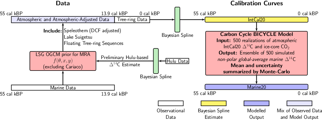
Figure 1 Schematic diagram of IntCal20 and Marine20 age calibration curve construction. IntCal20 is based solely upon tree-ring measurements from 0 to ca. 13.9 cal kBP. Beyond this a variety of data are used, including marine records which require an initial transformation to an atmospheric equivalent. To achieve this, a preliminary Δ14C history is estimated based upon Hulu Cave speleothems (Southon et al. Reference Southon, Noronha, Cheng, Edwards and Wang2012; Cheng et al. Reference Cheng, Edwards, Southon, Matsumoto, Feinberg, Sinha, Zhou, Li, Li and Xu2018). This preliminary Δ14C curve is used to drive the LSG OGCM and provide prior, first-order, estimates of regional MRAs (Butzin et al. Reference Butzin, Köhler, Heaton and Lohmann2020 in this issue) for each IntCal20 marine dataset, with the exception of the Cariaco Basin which is adjusted adaptively during curve construction (Hughen and Heaton Reference Hughen and Heaton2020 in this issue). The adjusted marine data are then combined with speleothems, macrofossils from Lake Suigetsu, and floating tree-ring sequences to constitute a mixed, atmospheric and atmospheric-adjusted, dataset extending from ca. 13.9–55 cal kBP. A Bayesian spline is jointly fitted to both the tree-ring samples (from 0–13.9 cal kBP) and this mixed data (beyond 13.9 cal kBP) to create the IntCal20 curve (Heaton et al. Reference Heaton, Blaauw, Blackwell, Bronk Ramsey, Reimer and Scott2020 in this issue). To generate Marine20, 500 posterior atmospheric Δ14C realizations are taken from the IntCal20 Bayesian spline and propagated through the BICYCLE carbon cycle model alongside reconstructions of atmospheric CO2 obtained from ice core records. The ensemble of 500 simulated outputs are then summarized to create the Marine20 curve.
The proposed modeling approach offers a significant improvement over previous marine calibration curves, e.g. Marine04 (Hughen et al. Reference Hughen, Baillie, Bard, Beck, Bertrand, Blackwell, Buck, Burr, Cutler, Damon, Edwards, Fairbanks, Friedrich, Guilderson, Kromer, McCormac, Manning, Bronk Ramsey, Reimer, Reimer, Remmele, Southon, Stuiver, Talamo, Taylor, van der Plicht and Weyhenmeyer2004), Marine09 (Reimer et al. Reference Reimer, Baillie, Bard, Bayliss, Beck, Blackwell, Bronk Ramsey, Buck, Burr, Edwards, Friedrich, Grootes, Guilderson, Hajdas, Heaton, Hogg, Hughen, Kaiser, Kromer, McCormac, Manning, Reimer, Richards, Southon, Talamo, Turney, van der Plicht and Weyhenmeyer2009) and Marine13 (Reimer et al. Reference Reimer, Bard, Bayliss, Beck, Blackwell, Bronk Ramsey, Buck, Cheng, Edwards, Friedrich, Grootes, Guilderson, Haflidason, Hajdas, Hatté, Heaton, Hoffmann, Hogg, Hughen, Kaiser, Kromer, Manning, Niu, Reimer, Richards, Scott, Southon, Staff, Turney and van der Plicht2013). In these previous versions, the curves were generated in distinct sections and spliced together. For Marine13, the curve from 0–10.5 cal kBP was created using a time-invariant ocean-atmosphere box diffusion model (Oeschger et al. Reference Oeschger, Siegenthaler, Schotterer and Gugelmann1975) driven by the corresponding atmospheric IntCal13 pointwise means and a range of piston velocities and eddy diffusivities as described in Hughen et al. (Reference Hughen, Baillie, Bard, Beck, Bertrand, Blackwell, Buck, Burr, Cutler, Damon, Edwards, Fairbanks, Friedrich, Guilderson, Kromer, McCormac, Manning, Bronk Ramsey, Reimer, Reimer, Remmele, Southon, Stuiver, Talamo, Taylor, van der Plicht and Weyhenmeyer2004). From 10.5–13.9 cal kBP, it was constructed based upon marine observations from a range of locations. Finally, beyond 13.9 cal kBP, Marine13 was identical to the atmospheric IntCal13 curve with a constant MRA offset of 405 14C yr.
Conversely, for Marine20, the use of BICYCLE and of time-dependent forcings permit more complex and realistic inclusion of key carbon cycle changes extending back to 55 cal kBP. Additionally, improvements in the Bayesian modeling of IntCal20 (Heaton et al. Reference Heaton, Blaauw, Blackwell, Bronk Ramsey, Reimer and Scott2020 in this issue) allow us for the first time to rigorously incorporate the time-dependent uncertainty of atmospheric Δ14C into the marine age calibration curve through our Monte-Carlo approach. Together, these features enable more accurate estimation of both the global marine calibration curve and the globally averaged MRA, especially beyond the Holocene. We show that the results BICYCLE provides for individual runs are almost indistinguishable from the three dimensional Large Scale Geostrophic Ocean General Circulation Model (LSG OGCM) (Butzin et al. Reference Butzin, Köhler and Lohmann2017, Reference Butzin, Köhler, Heaton and Lohmann2020 in this issue) and that BICYCLE’s model output agrees well with pre-bomb data based on seawater (Bard Reference Bard1988) and marine shells (Reimer and Reimer Reference Reimer and Reimer2001; Toggweiler et al. Reference Toggweiler, Druffel, Key and Galbraith2019).
While more complex ocean models such as the LSG OGCM exist, we deliberately retain the simpler BICYCLE box model since it is more appropriate for our specific, global-average, calibration needs. For practical radiocarbon calibration, we require not only a curve consisting of a single point estimate for the global marine Δ14C at any calendar age but also a reliable measure of the uncertainty on that estimate. The use of the computationally fast BICYCLE box model allows us to create a large ensemble of simulations and hence, via Monte-Carlo, rigorously quantify the uncertainty in the modeled global-average marine Δ14C level which is a necessary consequence of the uncertainty in our various model/climate inputs.
The paper is set out as follows. In Section 2 we describe the requirements for a computer model in order to be suitable for use in construction of a radiocarbon age calibration curve; how uncertainty in the various driving inputs can be propagated through such a computer model; and provide a short tutorial on how the resultant output uncertainty can be quantified using Monte-Carlo techniques as well as why these Monte-Carlo techniques are needed. In Section 3, we justify our recommended approach to marine calibration of using local ΔR adjustments, based upon observations, to a global-average curve rather than directly using regional output from more complex three-dimensional models. In Section 4 we present a short summary of BICYCLE and describe in detail the key processes/forcings and their uncertainties which we propagate through to our final calibration curve. We generate our ensemble of 500 BICYCLE simulations across the plausible ranges of its key inputs and present the resultant Marine20 curve in Section 5. Here we also discuss differences with the previous Marine13 curve. In particular, we note that Marine20 estimates a significant, and consistent, increase in the globally averaged MRA when compared to Marine13. With a sensitivity analysis we also document how much the different processes contribute to the overall uncertainty in Marine20. Section 6 provides a comparison against simulations with the more complex LSG OGCM and against both current day (pre-bomb) global marine data and older marine data from the IntCal20 database. Here we show that the increase, when compared to Marine13, in the global-average MRA in Marine20 is in agreement with average pre-bomb observations and the LSG OGCM. Finally, in Section 7 we discuss the limitations of our approach alongside areas needed for future work and development. For those seeking further details on the model output, including the final Marine20 radiocarbon age calibration curve, the spatially resolved regional open-ocean MRA estimates from the LSG OGCM, as well as the 500 NH atmospheric Δ14C realizations used as inputs for our Monte-Carlo ensemble, see PANGAEA (https://doi.org/10.1594/PANGAEA.914500).
For a calibration end-user, it is key to note that the update from Marine13 to Marine20 is accompanied by updates to the regional ΔR corrections which can be found at http://calib.org/marine/. This is particularly critical since Marine20 estimates a significantly increased globally averaged MRA. Calibration of local reservoirs using values of ΔR based on Marine13 will give incorrect calendar age estimates.
Calibration in Polar Regions
Our Marine20 curve is intended for calibration of marine 14C samples arising from non-polar locations, nominally/approximately ranging from 40ºS–40/50ºN. In higher-latitude polar regions, MRAs and critically their possible fluctuations over time are expected to be larger due to significantly increased variability in ocean ventilation and air-sea gas exchange mostly arising from changes in sea ice extent and differences in wind strength (Butzin et al. Reference Butzin, Prange and Lohmann2005). This is particularly likely to be the case during glacial periods. LSG OGCM estimates for the MRA in a particular calendar year within polar regions can vary by over 1000 14C yr between a simulation assuming a climate scenario suitable for the present day (its PD scenario which assumes little sea ice, Butzin et al. Reference Butzin, Prange and Lohmann2005, Reference Butzin, Köhler, Heaton and Lohmann2020 in this issue) and runs in climate scenarios appropriate for more extreme glacial periods (e.g. its GS/CS scenarios where the extent of sea ice is much greater in addition to significant changes to ocean ventilation and wind stress). This difference indicates that uncertainty in past polar climate conditions can have a significant effect on calibration in these regions. Consequently, for those polar regions affected by such additional variability, an assumption of a constant ΔR adjustment from our equatorial Marine20 global-average is not suitable. The current Marine20 curve is not therefore suitable for calibration in these polar regions.
Current proxy records for such ocean ventilation, sea ice extent and wind strength are not sufficient to reliably reconstruct these variables to permit accurate and precise modeling of polar calibration curves. Construction of such polar curves would be a valuable area for future study which we discuss in more detail within Section 7. For current users wishing to calibrate marine 14C samples from polar locations where variability in sea ice and ocean circulation may have significantly affected MRAs, we direct them to the regional LSG OGCM output as discussed in Section 3 and available on PANGAEA. Such users should however be aware that each individual LSG OGCM simulation only considers a single climate scenario. Due to the very considerable uncertainty on the appropriate historic polar climatic conditions, and since the impact of different climate scenarios on MRA in these regions is very large, resultant polar calibration based upon such fixed scenarios should be treated with extreme caution. The calibrated age estimates obtained under any single fixed scenario are likely to be considerably over-precise.
2. THE MONTE-CARLO PRINCIPLE OF MARINE20 CURVE CONSTRUCTION
A Computer Model
The use of models for the study and prediction of MRA extends back to Craig (Reference Craig1957), Arnold (Reference Arnold1957), Revelle and Suess (Reference Revelle and Suess1957) and was updated later by Oeschger et al. (Reference Oeschger, Siegenthaler, Schotterer and Gugelmann1975) with the introduction of a diffusion coefficient to simulate mixing in the deep ocean box (eddy diffusivity). This so-called box-diffusion model has been fundamental to the construction of the marine radiocarbon age calibration curve since 1986 (Stuiver et al. Reference Stuiver, Pearson and Braziunas1986). Over that time, the complexity of these models has increased as we have gained more knowledge of both the Earth systems and past climate constraints. Recent approaches include more advanced carbon cycle box models which allow transient forward simulations such as BICYCLE (Köhler et al. Reference Köhler, Muscheler and Fischer2006) through to full three-dimensional ocean general circulation models such as the LSG OGCM (Butzin et al. Reference Butzin, Prange and Lohmann2005, Reference Butzin, Prange and Lohmann2012, Reference Butzin, Köhler and Lohmann2017, Reference Butzin, Köhler, Heaton and Lohmann2020 in this issue). For all of these models, the basic principle is the same: given a specific user-defined set of inputs/parameters, they provide an estimate/prediction of the variable of interest, in our case the non-polar global-average marine Δ14C, where this average in the following is restricted to the area between 40°S and either 50°N (Atlantic) or 40°N (Pacific) to avoid the potential complications of including regions covered with sea ice (e.g. Butzin et al. Reference Butzin, Köhler and Lohmann2017).
The most useful computer model for a particular situation will depend upon the specific question one wishes to answer. For Marine20, we wish to not only obtain a reliable estimate of the global-average marine 14C concentration over time incorporating known changes in both the carbon cycle and atmospheric 14C production rate, but also to be able to quantify our uncertainty on that estimate. Such quantification of uncertainty is fundamental to radiocarbon calibration. When calibrating a radiocarbon date, we need not only a best “point estimate” for its calendar age but also a plausible range, i.e. to understand the uncertainty on our calibrated calendar age. These two competing aims of reliability and uncertainty quantification typically require a trade-off in model selection. We require a computer model that can incorporate desired physical processes and changes to the carbon cycle that proxy data tell us occurred; and yet also allows us to understand and propagate model uncertainty, specifically in the values of the input parameters, through to the final marine Δ14C estimate. In the case of our chosen BICYCLE computer model, the various inputs are illustrated in Figure 2.
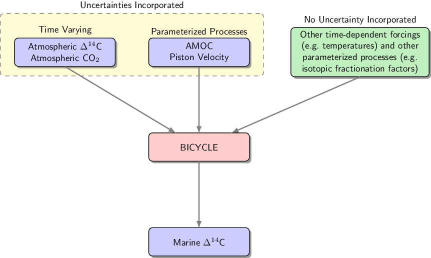
Figure 2 Propagating uncertainty through the BICYCLE model. For each simulation, we generate different inputs for BICYCLE by drawing from the variables on which we consider uncertainty (shown in the yellow box). AMOC denotes the Atlantic meridional overturning circulation and piston velocity the rate of air-sea gas exchange, see Section 4 for further details. These random inputs are combined with the inputs for which no uncertainties are incorporated (shown in green) and entered into the BICYCLE model. Each simulation of BICYCLE therefore provides a different, deterministic historic global-average estimate of marine surface Δ14C from 0–55 cal kBP. From the resulting ensemble we generate a Monte Carlo estimate of the mean and variance at any calendar age which is then used for the Marine20 radiocarbon age calibration curve.
A Brief Introduction to Quantifying Model Uncertainty
The majority of computer models simulating changes in the carbon cycle are deterministic. This means that they do not internally introduce randomness—if one drives the model with the same inputs one will always get identical outputs. Let us assume that such a computer model takes as inputs a range/vector of parameters φ which we specify. In our context, these model parameters are any input needed by the model—they could be a forcing, a user chosen setting or a tuned variable. In the case of marine 14C reservoir age simulations, these input parameters typically include the historic levels of atmospheric Δ 14C and CO2 concentration; ocean circulation; and air-sea gas exchange amongst others. Having specified values for these inputs, the model prediction at any calendar age θ is then represented by the deterministic function f(θ; φ).
In the case of a deterministic computer model, output uncertainty arises from two sources (see Section 2 of Kennedy and O’Hagan Reference Kennedy and O’Hagan2001). The first is model parameter uncertainty, i.e. that, typically, we do not know the true value of the model’s input parameters. We specify our uncertainty on our computer model inputs in terms of a distribution  $\phi \sim \pi \left( \phi \right)$ that encapsulates our current understanding about their values. The second source of uncertainty is model discrepancy, i.e. that any computer model is not an entirely accurate representation of reality and will not capture the complete carbon cycle of the Earth. This type of uncertainty is much harder to evaluate but one might expect a more complex and detailed model to typically have a smaller model discrepancy. We do not attempt to formally incorporate model discrepancy into Marine20 but we are able to incorporate model parameter uncertainty.
For calibration purposes, we wish to estimate, for any calendar age θ both the expectation  ${\mu _{Mar}}\left( \theta \right)$ and the variance $\sigma _{Mar}^2\left( \theta \right)$ in the global-average level of marine $\Delta _{MarineAv}^{14}C\left( \theta \right)$. To propagate our model parameter uncertainty, we therefore need to evaluate both:
 $${\mu _{Mar}}\left( \theta \right) = E\left[ {\Delta _{MarineAv}^{14}C\left( \theta \right)} \right] = \int f\left( {\theta ;\phi } \right)\pi \left( \phi \right)d\phi ,$$
and
 $$\sigma _{Mar}^2\left( \theta \right) = Var\left[ {\Delta _{MarineAv}^{14}C\left( \theta \right)} \right] = {\rm{ }}\left\{ {\int {{f^2}} \left( {\theta ;\,\phi } \right){\rm{ }}\pi \left( \phi \right)d\phi } \right\}{\rm{ }} - \mu _{Mar}^2\left( \theta \right),$$
Where  $\pi \left( \phi \right)$ is the density of the model’s input parameters that specifies our prior beliefs/uncertainties about their true values, and f(θ; φ) is the model output at calendar year θ cal kBP when it has been run with specific inputs φ.
Monte-Carlo Estimation
Due the complexity of the computer model, it is not possible to calculate either of these integrals explicitly, but we can estimate them via a Monte-Carlo approach. To do so, we sample a range of N plausible inputs φ 1, …, φN from our density $\pi \left( \phi \right)$. The model is then run with each of these inputs giving us a large ensemble of N outputs  $f\left( {\theta ;{\phi _1}} \right), \ldots ,f\left( {\theta ;{\phi _N}} \right)$. The sample mean and variance of this ensemble then provide estimates for ${\mu _{Mar}}\left( \theta \right)$ and $\sigma _{Mar}^2\left( \theta \right)$ respectively, i.e. we estimate
 $${\hat \mu _{Mar}}\left( \theta \right) = {1 \over N}\mathop \sum \limits_{i=1}^N f\left( {\theta ;{\phi _i}} \right)\;{\rm{and}}$$
 $$\hat \sigma _{Mar}^2\left( \theta \right) = {\rm{}}{1 \over {N - 1}}\mathop \sum \limits_{i = 1}^N {\left( \,{f\left( {\theta ;{\phi _i}} \right) - {{\hat \mu }_{Mar}}\left( \theta \right)} \right)^2},\;{\rm{where}}\;{\rm{each}}\,{{\phi}_i}\,\,\sim\,\,\,\,\pi (\phi ).$$
Importantly, as most computer models are highly non-linear, we stress that only running them at extreme “end-member” inputs is not sufficient to reliably represent output uncertainty. Equally, running a computer model with the value of an input parameter set at its mean is not sufficient to estimate the mean of the output when input parameter uncertainty is properly incorporated. Both these points are illustrated with a simple example in the next subsection.
To perform accurate Monte-Carlo estimation, it is necessary to generate a sufficiently large ensemble N of outputs in order that they provide reliable estimates. Here, we selected N=500 based on a smaller pilot study which indicated such a sample size would provide Monte-Carlo estimates that were within ±1% of the true model mean, and ±5% of the true model variance. This requires repeated model simulations and so it is necessary to have a model that is sufficiently fast to permit this. BICYCLE provides an appropriate compromise between reducing model discrepancy while still running with sufficient computational speed to enable creation of a large ensemble of outputs and hence accurately propagate model parameter uncertainty. As we show later in Figure 4 and Section 6, there are only small differences between the global-average MRA obtained from individual BICYCLE simulations and from the more complex 3D LSG OGCM alternative, yet each BICYCLE simulation can be performed in seconds rather than the weeks required for the LSG OGCM.
Finally, we note that, as described in Heaton et al. (Reference Heaton, Blaauw, Blackwell, Bronk Ramsey, Reimer and Scott2020 in this issue) laying out the statistical methodology for the atmospheric calibration curve, one could calibrate directly against the ensemble of N model outputs if covariance information on the marine calibration curve is desired. However, since current calibration tools use pointwise calibration curve means and variances, we do not discuss this further here.
A Toy Monte-Carlo Example
To illustrate the need for the Monte-Carlo approach, if we wish to accurately estimate the mean output of a computer model and capture the model uncertainty, we consider a simple example. While somewhat pathological it does illustrate the key points that running a computer model at the extreme values of its inputs does not ensure we have captured the full uncertainty in the model output; and also that setting the inputs at their mean values does not result in the mean model output.
Specifically, let us suppose we have a computer model that takes a single input x and returns the value  $g\left( x \right) = {x^2}$. Further, assume that we do not know x but can quantify our prior belief that it lies uniformly between −1 and 1, i.e. $X \sim Unif\left[ { - 1,1} \right]$. With such a simple model we can work out exactly what the distribution of the outputs should be. This is shown by the solid blue line in Figure 3. All values in the range [0,1] are clearly possible outputs. Further, we can calculate the true mean output $E\left[ {g\left( X \right)} \right] = {1 \over 3}$ (dot-dashed blue line).
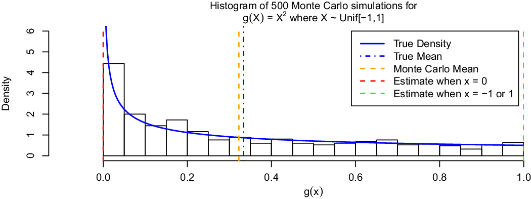
Figure 3 Toy example to illustrate the need for the Monte Carlo approach to accurately estimate both the mean and variability in the output of a computer model.
However, if we run the model at the extreme ends of its possible inputs (either x=1 or −1), in both cases we observe the output g(x) = 1 (green dashed line). If we were to assume that these end-member outputs, generated by the extreme inputs, informed us about the full range of potential outputs then we would falsely assume that the output of the model had no uncertainty. Similarly, to find the true mean of the model output we cannot simply run the model with the input x set to its mean value, i.e. E(X] = 0. Doing so would provide the output g(0) = 0 (red dashed line) rather than the correct mean of  ${1 \over 3}$.
On the other hand, if we create a Monte Carlo sample of 500 independent ${X_i} \sim Unif\left[ { - 1,1} \right]$ values and propagate each of these through the model we obtain the ensemble of outputs shown by the histogram. Comparing this against the true output density in solid blue, we can see that our random ensemble is able to capture the correct uncertainty in the model’s output. Further, the mean of these 500 outputs (orange dashed line) shows that, by Monte-Carlo, we are able to accurately estimate the true mean output.
3. WHY DO WE NEED A MONTE CARLO APPROACH AND WHY ARE WE NOT USING REGIONAL 4D OGCM OUTPUT DIRECTLY?
Why Do We Need Monte-Carlo for Marine20?
To be of use for calibration, it is essential to accurately represent the full range of uncertainty in the level of marine radiocarbon. When calibrating a radiocarbon determination, we need to discover all calendar ages which are potentially consistent with that level of 14C. As such we are required to understand the variability in the output of our, complex and non-linear, carbon cycle computer model. This is somewhat different from much modeling which aims to test specific scenarios. As described in Section 2, in order to capture the full variability in the computer model output we must explore the full range of input scenarios. Understanding this uncertainty in computer model output requires us to consider not just the extremes but also those intermediate scenarios, i.e. a Monte Carlo approach.
Limitations of a Constant ΔR Approach
It is expected that the most significant temporal changes in MRA will be shared and hence occur on a global scale rather than in individual regions, i.e. changes in values over time will predominantly be seen in ${R^{GlobalAv}}\left( \theta \right)$ as opposed to the regional ΔR(θ) adjustments (Stuiver et al. Reference Stuiver, Pearson and Braziunas1986). These global-scale MRA changes are incorporated, by construction, in our global-average Marine20 curve and hence automatically taken into account for all calibration users wishing to use the Marine20 curve.
However, in assuming a constant ΔR we do not permit for potential smaller region-specific temporal changes. This assumption of temporally invariant ΔR values should be adopted with caution in the context of a changing climate and a changing marine carbon cycle. Any global marine radiocarbon calibration product that makes use of modern ΔR values should therefore be used with similar caution.
How Were Marine Data Incorporated into IntCal20?
For time periods where sufficient tree-ring 14C determinations exist, i.e. continuously from 0–13,913 cal BP, no marine data were used in the creation of the IntCal20 curve. Further back in time however, marine observations did contribute alongside speleothems, floating tree rings and macrofossils from Lake Suigetsu (see Figure 1 and Reimer et al. Reference Reimer, Austin, Bard, Bayliss, Blackwell, Bronk Ramsey, Butzin, Cheng, Edwards, Friedrich, Grootes, Guilderson, Hajdas, Heaton, Hogg, Hughen, Kromer, Manning, Muscheler, Palmer, Pearson, van der Plicht, Reimer, Richards, Scott, Southon, Turney, Wacker, Adophi, Büntgen, Capano, Fahrni, Fogtmann-Schulz, Friedrich, Kudsk, Miyake, Olsen, Reinig, Sakamoto, Sookdeo and Talamo2020 in this issue). To incorporate this marine data into the atmospheric IntCal20, estimates of the MRA for each constituent datum were required. With the exception of Cariaco Basin (Hughen and Heaton Reference Hughen and Heaton2020 in this issue), for which a different approach was taken due to its unusual topography, to obtain these MRA estimates the following approach was taken.
To begin, an interim atmospheric 14C curve based upon only the Hulu Cave speleothems (Southon et al. Reference Southon, Noronha, Cheng, Edwards and Wang2012; Cheng et al. Reference Cheng, Edwards, Southon, Matsumoto, Feinberg, Sinha, Zhou, Li, Li and Xu2018) was constructed using the same Bayesian spline with errors-in-variables methodology as the final IntCal20 curve (Heaton et al. Reference Heaton, Blaauw, Blackwell, Bronk Ramsey, Reimer and Scott2020 in this issue). This interim Hulu-based 14C history was then entered as a forcing to the LSG OGCM to get the coarse regional MRA estimates under its GS scenario (Butzin et al. Reference Butzin, Köhler, Heaton and Lohmann2020 in this issue) shown in Figure 3 of Reimer et al. (Reference Reimer, Austin, Bard, Bayliss, Blackwell, Bronk Ramsey, Butzin, Cheng, Edwards, Friedrich, Grootes, Guilderson, Hajdas, Heaton, Hogg, Hughen, Kromer, Manning, Muscheler, Palmer, Pearson, van der Plicht, Reimer, Richards, Scott, Southon, Turney, Wacker, Adophi, Büntgen, Capano, Fahrni, Fogtmann-Schulz, Friedrich, Kudsk, Miyake, Olsen, Reinig, Sakamoto, Sookdeo and Talamo2020 in this issue).
Since LSG OGCM estimates are intended for the open-ocean as opposed to the more coastal locations of the marine IntCal20 data, a further constant coastal radiocarbon reservoir age adjustment/shift was however required. For each marine dataset, an independent prior was placed on this required coastal shift based upon the observed offset between the 14C ages of the more recent observations from that specific marine dataset and IntCal20’s atmospheric dendrodated trees (which extend back to ca. 14,190 cal BPFootnote 2).
Intuitively, this coastal shift approach used the relative changes (i.e. the shape) in the regional LSG OGCM open-ocean MRA estimates but not their absolute values. The internally estimated coastal shift is equivalent to estimating a temporally invariant pseudo-ΔR for the specific coastal location relative to the nearby open-ocean. These coastal pseudo-ΔR shifts from the GS scenario of LSG OGCM ranged from approximately 12 14C yr in Vanuatu up to over 280 14C yr in Kiritimati indicating the difficulty in using open-ocean OGCM estimates directly for coastal data.
These preliminary Hulu-Cave based MRA estimates are expected to be overly smooth (since they are based upon the relatively smooth Hulu Cave record) however they should provide robust first-order approximations that enable marine data to contribute to IntCal20. The region-specific prior MRA estimates were then used as inputs for the Bayesian approach to IntCal20’s curve construction allowing for some further fine-scale MRA variability not captured by the coarse preliminary Hulu-based estimates. In this curve construction process, the coastal shift priors were further updated to resolve differences between the diverse pre-Holocene data sets, see Heaton et al. (Reference Heaton, Blaauw, Blackwell, Bronk Ramsey, Reimer and Scott2020 in this issue) for complete details.
Importantly, as shown in Figure 3 of Reimer et al. (Reference Reimer, Austin, Bard, Bayliss, Blackwell, Bronk Ramsey, Butzin, Cheng, Edwards, Friedrich, Grootes, Guilderson, Hajdas, Heaton, Hogg, Hughen, Kromer, Manning, Muscheler, Palmer, Pearson, van der Plicht, Reimer, Richards, Scott, Southon, Turney, Wacker, Adophi, Büntgen, Capano, Fahrni, Fogtmann-Schulz, Friedrich, Kudsk, Miyake, Olsen, Reinig, Sakamoto, Sookdeo and Talamo2020 in this issue), for locations of the marine data used for making IntCal20, the relative differences in the shapes of the Hulu-based regional open-ocean MRA estimates provided by the LSG OGCM were small (in the order of ±5% of the absolute value of MRA). Furthermore, these regional open-ocean MRA estimates had similar shapes to the non-polar global-average MRA. Hence, in terms of the final MRAs used for the marine data contributing to IntCal20, there would be little difference in having applied individual temporally invariant coastal shifts to the non-polar global-average MRA (i.e. the approach we recommend for Marine20 to restrict temporal changes in MRA to the global-average) of the LSG OGCM rather than the region-specific output. Our proposed global-average Marine20 approach to calibration is therefore consistent with that taken to integrate the marine data into IntCal20.
Why Not Use OGCM Output Directly to Provide Regional Calibration Curves?
Much of the marine data which users wish to calibrate come from coastal regions. With our current state of knowledge, most global OGCMs do not have the resolution to simulate these coastal regions accurately and their results may be flawed at such sites. This includes the LSG OGCM. We are therefore still recommending, for the current update, the use of a global-average radiocarbon age calibration curve with the adjustment of a constant ΔR estimated independently based upon the offset between local observations and the Marine20 curve.
In Figure 4, we plot the pre-Holocene LSG OGCM regional open-ocean MRA estimates obtained when forced by the pointwise mean of the final IntCal20 curve (Reimer et al. Reference Reimer, Austin, Bard, Bayliss, Blackwell, Bronk Ramsey, Butzin, Cheng, Edwards, Friedrich, Grootes, Guilderson, Hajdas, Heaton, Hogg, Hughen, Kromer, Manning, Muscheler, Palmer, Pearson, van der Plicht, Reimer, Richards, Scott, Southon, Turney, Wacker, Adophi, Büntgen, Capano, Fahrni, Fogtmann-Schulz, Friedrich, Kudsk, Miyake, Olsen, Reinig, Sakamoto, Sookdeo and Talamo2020 in this issue) under the GS scenario. These estimates are the closest LSG OGCM analogue to our Marine20 approach but do not incorporate any uncertainty propagation as Monte-Carlo is infeasible due to the LSG OGCM’s long run time. Shown are the LSG OGCM’s MRA estimates for the open-ocean sites lying closest to each of the marine locations used in IntCal20. Also shown are the LSG OGCM (50°S–50°N) globally averaged estimate with the same IntCal20 pointwise mean forcing and GS scenario, and also the Monte-Carlo mean of our BICYCLE/Marine20 globally averaged MRA discussed in detail later.
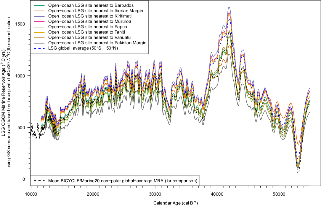
Figure 4 Regional open-ocean MRA estimates generated by the LSG OGCM when forced by the mean of the IntCal20 (Reimer et al. Reference Reimer, Austin, Bard, Bayliss, Blackwell, Bronk Ramsey, Butzin, Cheng, Edwards, Friedrich, Grootes, Guilderson, Hajdas, Heaton, Hogg, Hughen, Kromer, Manning, Muscheler, Palmer, Pearson, van der Plicht, Reimer, Richards, Scott, Southon, Turney, Wacker, Adophi, Büntgen, Capano, Fahrni, Fogtmann-Schulz, Friedrich, Kudsk, Miyake, Olsen, Reinig, Sakamoto, Sookdeo and Talamo2020 in this issue) reconstruction of NH atmospheric Δ14C. These estimates are obtained under LSG’s GS scenario (Butzin et al. Reference Butzin, Köhler, Heaton and Lohmann2020 in this issue) and correspond to the open-ocean sites nearest to the locations of the IntCal20 marine data. Also shown is the LSG (50°S–50°N) global-average MRA estimate in the GS scenario; and also the mean of BICYCLE’s global-average MRA for comparison.
A potential approach to adapt this open-ocean LSG OGCM output for calibration in wider and/or coastal locations would be that taken for inclusion of marine data in IntCal20. One would initially identify the regional open-ocean LSG OGCM site that lies closest to the particular location of interest, before then applying a constant, baseline-specific, pseudo-ΔR shift from this specific regional open-ocean LSG OGCM estimate. However, extending this approach to Marine20 would be complex and reliant upon users identifying both the correct LSG OGCM regional baseline and the matching pseudo-ΔR shift.
Furthermore, for the non-polar sites illustrated in Figure 4, the relative shapes of the regional open-ocean MRAs estimated by the LSG OGCM are highly similar to both the LSG global-average estimate and also the mean BICYCLE global-average estimate. Changing to two alternative scenarios (CS or PD, Butzin et al. Reference Butzin, Köhler, Heaton and Lohmann2020 in this issue) within the LSG OGCM also has little effect on the relative shapes of the resultant regional open-ocean MRA estimates—the primary effect of such scenario changes are simply constant shifts, up and down respectively, in each regional open-ocean MRA estimate albeit with the size of these shifts potentially varying between regions.
Consequently, the difference in using constant pseudo-ΔR-type shifts from regional LSG OGCM curves, as opposed to constant ΔR shifts from the global-average curves, would be small for these sites. As a result, the proposed approach to radiocarbon age calibration described here, of using a global-average Marine20 radiocarbon age calibration curve based on BICYCLE with application of constant ΔR shifts, is consistent with an approach using regional LSG OGCM curves while also being much simpler and more efficient.
As discussed in more detail in Section 6, the output from the LSG OGCM matches that from BICYCLE at the global-average level suggesting that BICYCLE is a satisfactory model at this broader scale. However, by running much more quickly than the full LSG OCGM, BICYCLE provides greatly more flexibility which provides several key benefits for our calibration curve needs. In particular, LSG (or any other current OGCM) is too computationally expensive to carry out a rigorous exploration of the uncertainty in its output. The use of BICYCLE enables us to explore a much wider range of potential carbon cycle scenarios. Further, the LSG OGCM simulations were kept in a single scenario for the entire period from 0–55 cal kBP. The effect of a transient switch from a glacial scenario to an interglacial, more suitable for the Holocene, within a simulation was therefore unknown. With BICYCLE we can more easily investigate the effect of such scenario changes.
Our BICYCLE approach attempts to minimise potential inaccuracies in marine radiocarbon variability that stem from strictly unknown changes in the marine carbon cycle by exploring a wide range of possible carbon cycle states, providing a trade-off between expected accuracy and precision in resulting calibrated ages. As we describe later in Section 7, key future work lies in developing 3D OGCM models which can provide region-specific output further and understanding their inherent uncertainties. Work towards this goal would be invaluable in improving both marine calibration and our insight into the global carbon cycle.
Users calibrating open-ocean samples who wish to use individual regional MRA estimates provided by the LSG OGCM can find them on PANGAEA (https://doi.org/10.1594/PANGAEA.914500). This may also be relevant for users wishing to calibrate data outside Marine20’s intended range, i.e. where sea ice may have been present (north of 40/50°N or south of 40°S), especially if the LSG OGCM estimates exhibit significantly different relative changes. One approach to incorporate LSG OGCM MRA estimates, for example into OxCal, can be found via Alves et al. (Reference Alves, Macario, Urrutia, Cardoso and Bronk Ramsey2019).
4. BICYCLE—THE BOX MODEL OF THE ISOTOPIC CARBON CYCLE
BICYCLE is a global carbon cycle box model that includes terrestrial, atmospheric and oceanic modules (Köhler and Fischer Reference Köhler and Fischer2004; Köhler et al. Reference Köhler, Fischer, Munhoven and Zeebe2005). The terrestrial biosphere is modeled with seven different compartments distinguishing C3 and C4 photosynthesis, and soils with different turnover times; the atmosphere as a single globally averaged box; and the ocean as a set of ten boxes covering different spatial regions (both equatorial and high latitude) and ocean depths including deep ocean-sediment exchange fluxes. Prognostic variables solved by the model are C (as DIC in the ocean, as CO2 in the atmosphere), 13C, and 14C in all boxes, and additionally alkalinity, O2, and PO4 in the ocean. The marine carbonate system is fully defined by the two variables DIC and alkalinity. The model design has been chosen to allow long-term (thousands of years) transient simulations, but still capture the essential processes important for the global carbon cycle and carbon isotopes. Temporal changes in the physical boundary conditions (temperature, ocean circulation, sea ice extent, sea level, aeolian dust/iron input, 14C production rate) are prescribed, and thus changes in the simulated subsystem of the global carbon cycle are externally forced. In past studies covering Termination I, the last glacial cycle, or the past 740 kyr (Köhler et al. Reference Köhler, Fischer, Munhoven and Zeebe2005, Reference Köhler, Muscheler and Fischer2006, Reference Köhler, Fischer and Schmitt2010, Reference Köhler, Knorr and Bard2014; Köhler and Fischer Reference Köhler and Fischer2006) BICYCLE has been used to reproduce (simulate) reconstructed variables of the carbon cycle, such as atmospheric CO2, 13C, and 14C.
The version of BICYCLE used here is based on Köhler et al. (Reference Köhler, Muscheler and Fischer2006), in which a previous attempt to simulate the changes in atmospheric Δ14C over the last 50 cal kBP documented in IntCal04 has been published. For our current Marine20 application, the following model improvements with respect to that earlier application have been implemented:
In Köhler et al. (Reference Köhler, Muscheler and Fischer2006) sediment-deep ocean fluxes of DIC and alkalinity were prescribed by temporal change in the depth of the lysocline. The representation of sediment-deep ocean fluxes was revised in Köhler and Fischer (Reference Köhler and Fischer2006) to a scheme that mimics the process of carbonate compensation (Broecker and Peng Reference Broecker and Peng1987) in a time-delayed response function to changes in deep ocean carbonate ion concentration. This response function approach has been used in all later applications of BICYCLE and is also applied here.
Atmospheric CO2 in the standard BICYCLE setup is a prognostic variable, i.e. is internally calculated rather than externally forced/prescribed. BICYCLE’s simulated CO2 time series has been in reasonable agreement with ice core data, but never matched them perfectly. However, for our current application we have decided to override BICYCLE’s internal CO2 estimates and instead prescribe CO2 from ice core data (Figure 5, based on Köhler et al. Reference Köhler, Nehrbass-Ahles, Schmitt, Stocker and Fischer2017). This decision was made since the air-sea gas exchange, one of the key processes determining the simulated surface ocean Δ14C, is significantly dependent on the atmospheric concentration of CO2. In making this change, the internally calculated carbon cycle is partly corrected by an additional source/sink term in the atmosphere to arrive at the prescribed ice core reconstructed CO2 value. This is a common approach in carbon cycle model applications for future scenarios, in which not CO2 emissions, but CO2 concentrations are prescribed, and has recently been implemented in BICYCLE for its contribution to a carbon cycle model-intercomparison (Keller et al. Reference Keller, Lenton, Scott, Vaughan, Bauer, Ji, Jones, Kravitz, Muri and Zickfeld2018).

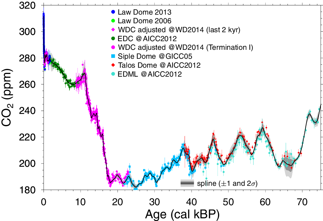
Figure 5 Atmospheric CO2 concentration used to force the BICYCLE model. Underlying ice core data and corresponding fitted spline are plotted for 0–75 cal kBP (modified from Köhler et al. Reference Köhler, Nehrbass-Ahles, Schmitt, Stocker and Fischer2017).
Atmospheric Δ14C, which was also a prognostic variable in previous versions of BICYCLE, is now also prescribed from data by individual realizations of NH atmospheric Δ14C taken from the Bayesian posterior of IntCal20 (Reimer et al. Reference Reimer, Austin, Bard, Bayliss, Blackwell, Bronk Ramsey, Butzin, Cheng, Edwards, Friedrich, Grootes, Guilderson, Hajdas, Heaton, Hogg, Hughen, Kromer, Manning, Muscheler, Palmer, Pearson, van der Plicht, Reimer, Richards, Scott, Southon, Turney, Wacker, Adophi, Büntgen, Capano, Fahrni, Fogtmann-Schulz, Friedrich, Kudsk, Miyake, Olsen, Reinig, Sakamoto, Sookdeo and Talamo2020 in this issue). Here, 14C production rates are simply adapted to match prescribed Δ14C values. Thus, no additional source term (as was necessary for CO2) has to be introduced.
Our model improvements of forcing atmospheric CO2 from external ice core data and atmospheric Δ14C by realizations of the IntCal20 curve aim to correct for any potential limitations in the BICYCLE model. These changes should bring the carbon cycle of the surface ocean closer to its true state than previous BICYCLE simulations where CO2 and atmospheric Δ14C were fully prognostic variables.
These new approaches of externally prescribing atmospheric CO2 and Δ14C manage to bring these variables in the model very close to (<1 ppm for CO2 and <1 ‰ for Δ14C) but not in full agreement with the prescribed time series. These minor differences remain because the prognostic variables in BICYCLE are determined through ordinary differential equations which are numerically solved with a 4th order Runge-Kutta method (Press et al. Reference Press, Teukolsky, Vetterling and Flannery1992). Such differences also prevent us from directly proposing how the 14C production rate should vary over time to be in agreement with IntCal20. Nevertheless, with more efforts in this direction it might, in the future, be possible to further constrain 14C production rate with atmospheric Δ14C by this approach.
Our simulations here are run over the last 75 cal kBP. Between 75 and 55 cal kBP, atmospheric Δ14C is kept fixed at its value for 55 cal kBP but CO2 and all other time-dependent forcings vary according to the data. These 20 kyr prior to 55 cal kBP give the radiocarbon cycle in BICYCLE reasonable time to adjust to the boundary conditions (for further details see Köhler et al. Reference Köhler, Muscheler and Fischer2006).
For Marine20, we consider the DIC-weighted mean of the simulated Δ14C of the equatorial surface ocean boxes as the non-polar global-average. These boxes are 100 m deep and range from 40°S to 50°N (Atlantic) or 40°N (Pacific).
Propagating Model Parameter Uncertainty through BICYCLE
While BICYCLE is a box model, it still contains a large number of parameters. To keep our approach practical, we focus our analysis of propagated model uncertainties on key processes and do not consider the uncertainty in all parameters. From sensitivity tests we identified that two processes are most important for simulated surface ocean Δ14C: piston velocity; and Atlantic meridional overturning circulation (AMOC), which is directly connected to the strength of North Atlantic Deep Water (NADW) formation.
Piston velocity is the rate of air-sea gas exchange and depends on near-surface wind speed. Thus, this parameter is important for the oceanic uptake of 14C from the atmosphere. In all previous applications, it was parametrized to 2.5 × 10⁻⁵ and 7.5 × 10⁻⁵ m s−1, for the equatorial and high latitude surface boxes respectively (Heimann and Monfray Reference Heimann and Monfray1989). These values agree reasonably well with more recent estimates (Wanninkhof Reference Wanninkhof2014). To create Marine20, we maintain these values as the mean piston velocities but introduce uncertainty by placing a prior on each informed by a meta-analysis as described below.
The strength of the AMOC in the model is important for the transport of tracers from the surface to the deep ocean via the physical carbon pump. In our Marine20 setup, the AMOC, represented by strength of the NADW formation, is considered to have two states with some uncertainty on the value in each state. In interglacials, it is centred around 16 Sv (1 Sverdrup = 106 m3 s−1, e.g. Talley et al. Reference Talley, Pickard, Emery and Swift2011) while during glacials it is centred at 10 Sv. See below for more details.
In addition to uncertainties in piston velocity and AMOC, we aim to propagate uncertainty on the past levels of atmospheric Δ14C and CO2. Below, we present a summary of how these various inputs were selected together with a description of their uncertainties. Those model parameters for which we consider uncertainty, and specify distributions on their values, are referred to as having uncertainty incorporated; while those for which we do not consider uncertainty are denoted as having uncertainty not incorporated. An overview of how these enter BICYCLE is given in Figure 2.
TIME DEPENDENT MODEL PARAMETERS FOR WHICH UNCERTAINTY IS INCORPORATED
Atmospheric Δ14C: for each BICYCLE simulation, we draw a distinct posterior realization of NH atmospheric Δ14C from the Bayesian spline of IntCal20 (Reimer et al. Reference Reimer, Austin, Bard, Bayliss, Blackwell, Bronk Ramsey, Butzin, Cheng, Edwards, Friedrich, Grootes, Guilderson, Hajdas, Heaton, Hogg, Hughen, Kromer, Manning, Muscheler, Palmer, Pearson, van der Plicht, Reimer, Richards, Scott, Southon, Turney, Wacker, Adophi, Büntgen, Capano, Fahrni, Fogtmann-Schulz, Friedrich, Kudsk, Miyake, Olsen, Reinig, Sakamoto, Sookdeo and Talamo2020 in this issue). Each of these realizations represent a different plausible past atmospheric history. To input into BICYCLE, they are sampled on a 10-calendar-year input grid and interpolated in-between. Using realizations in this way, as opposed to the pointwise IntCal20 curve summaries, allows us to incorporate not only our inherent uncertainty on the level of atmospheric Δ14C at any calendar age but also its smooth dependence over time. See Heaton et al. (Reference Heaton, Blaauw, Blackwell, Bronk Ramsey, Reimer and Scott2020 in this issue) for some illustrative atmospheric realizations over the Bølling-Allerød and further explanation on how these individual posterior realizations form the summarized IntCal20.
Atmospheric CO 2: our record of past atmospheric CO2 (Figure 5) is taken from a spline through ice core data as described in Köhler et al. (Reference Köhler, Nehrbass-Ahles, Schmitt, Stocker and Fischer2017). The spline estimate combines raw data from several different ice cores (Talos Dome, Siple Dome, WAIS Divide (WDC), EPICA Dome C (EDC), EPICA Dronning Maud Land (EDML) and Law Dome) each on the most recent age scale, e.g. AICC2012, GICC05, WD2014 (Ahn and Brook Reference Ahn and Brook2014; Ahn et al. Reference Ahn, Brook, Mitchell, Rosen, McConnell, Taylor, Etheridge and Rubino2012; Bauska et al. Reference Bauska, Joos, Mix, Roth, Ahn and Brook2015; Bereiter et al. Reference Bereiter, Lüthi, Siegrist, Schüpbach, Stocker and Fischer2012; Lüthi et al. Reference Lüthi, Bereiter, Stauffer, Winkler, Schwander, Kindler, Leuenberger, Kipfstuhl, Capron, Landais, Fischer and Stocker2010; MacFarling-Meure et al. Reference MacFarling-Meure, Etheridge, Trudinger, Langenfelds, van Ommen, Smith and Elkins2006; Marcott et al. Reference Marcott, Bauska, Buizert, Steig, Rosen, Cuffey, Fudge, Severinghaus, Ahn, Kalk, McConnell, Sowers, Taylor, White and Brook2014; Monnin et al. Reference Monnin, Indermühle, Dällenbach, Flückiger, Stauffer, Stocker, Raynaud and Barnola2001, Reference Monnin, Steig, Siegenthaler, Kawamura, Schwander, Stauffer, Stocker, Morse, Barnola, Bellier, Raynaud and Fischer2004; Rubino et al. Reference Rubino, Etheridge, Trudinger, Allison, Battle, Langenfelds, Steele, Curran, Bender, White, Jenk, Blunier and Francey2013). This fitted spline is accompanied by uncertainties that consider data resolution errors, Monte Carlo errors, and error due to a chosen cutoff period during smoothing leading to combined uncertainties in the spline,  ${\sigma _{C{O_2}}}\left( \theta \right)$. For each of the 500 realizations used as model inputs, we draw a Gaussian random variable ${x_i} \sim N\left( {0,{1^2}} \right)$ that defines the specific CO2 time series used as a forcing on simulation i,
 $$CO_2^i\left( \theta \right) = {\mu _{C{O_2}}}\left( \theta \right) + {x_i}{\sigma _{C{O_2}}}\left( \theta \right),$$
where  ${\mu _{C{O_2}}}\left( \theta \right)$ is the mean of the ice core spline at calendar age θ. This ensures that each individual CO2 forcing varies smoothly over time.
OTHER KEY PROCESS MODEL PARAMETERS FOR WHICH UNCERTAINTY IS INCORPORATED
As mentioned above, the two most influential processes for surface ocean Δ14C are piston velocity and AMOC (the strength of the NADW formation). Standard values have been taken for their means as in previous studies (e.g. Köhler et al. Reference Köhler, Fischer, Munhoven and Zeebe2005, Reference Köhler, Muscheler and Fischer2006) in which they have been justified. We specify uncertainties around these means, providing our reasoning below.
Piston Velocity:
Piston velocity is a key factor regulating the uptake of 14C by the ocean and hence largely determines simulated MRAs. Piston velocity depends on near-surface wind speed for which our knowledge is limited, in particular regarding values of the past. Therefore, piston velocities are perhaps the least well-constrained parameters in our model.
As stated above, BICYCLE operates with two piston velocities–dependent upon whether the surface ocean box falls in low or high-latitudes, which typically have either low or high wind speeds, respectively. Since BICYCLE has been tuned previously, and there is no common agreement on their absolute values, we do not change the mean values of these parameters as to do so would lead to a different carbon cycle baseline, potentially requiring further adjustments/analysis. We do however incorporate uncertainties around these means.
In specifying piston velocities and their uncertainties, we are not concerned with short-term, annual-scale, fluctuations. Short-term changes do not have a significant effect on the marine 14C reservoir since the slow air/ocean mixing process occurs over much longer time scales and so smooths such fine variations out. Instead, our interest is in quantifying the uncertainty in the long-term mean values. We model the piston velocities as constant over time and specify a ±15% (1σ) uncertainty on both the high-latitude and equatorial values:
 $${\rm{Equatorial \ Boxes}}\,\,{k_{Eq}} \sim N\left( {2.5 \times {{10}^{ - 5}},{{\left( {0.375 \times {{10}^{ - 5}}} \right)}^2}} \right){\rm{m}} \,{{\rm{s}}^{ - 1}},$$
 $${\rm{High - Latitude \ Boxes}}\,\,{k_{Hl}} \sim N\left( {7.5 \times {{10}^{ - 5}},{{\left( {1.125 \times {{10}^{ - 5}}} \right)}^2}} \right){\rm{m}} \,{{\rm{s}}^{ - 1}}.$$
Justification for Selection of Piston Velocity Uncertainties
To quantify historic piston velocity uncertainty, we first consider present day mean piston velocity with present day winds/climate. Naegler (Reference Naegler2009) provides five current day piston velocity estimates (with individual uncertainties) on comparable scales. We combine these values using a statistically rigorous meta-analysis (Figure 6) to give an estimate for the average present day piston velocity of  $\overline k \sim N\left( {17,{{1.4}^2}} \right)$ cm hr–1 (or equivalently N(4.7, 0.392) 10–5 m s–1), i.e. the 1σ uncertainty on the level of piston velocity with present day climate is approximately ±10%.
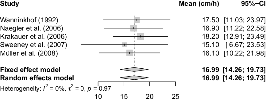
Figure 6 Meta-analysis of present-day estimates of piston velocity from Naegler (Reference Naegler2009). Shown are, post-Naegler’s adjustments, the piston velocities (cm hr–1) from 5 different studies together with their 95% confidence intervals (95%-CI). The grey diamonds represent the combined estimate, again with 95% intervals. Heterogeneity, as quantified by the measures  ${I^2},{\tau ^2}$ and p (Cochran’s Q-statistic), assesses the extent to which the reported velocities differ between the different studies, see e.g. Borenstein et al. (Reference Borenstein, Hedges, Higgins and Rothstein2011) for more details. Here, the five reported velocities are seen to be consistent with a single shared underlying velocity.
Further uncertainty arises as a result of changing past climate, in particular different wind speeds. From the LSG OGCM (Butzin et al. Reference Butzin, Köhler and Lohmann2017, Reference Butzin, Köhler, Heaton and Lohmann2020 in this issue) we obtain (Table 1) gas exchange rates based on 10-year averaged monthly model results for three different climate scenarios (PD, GS and CS, Butzin et al. Reference Butzin, Prange and Lohmann2005).
Table 1 Piston velocities for 14CO2 employed by the LSG OGCM according to various climate forcing scenarios, results are annual-mean values averaged over ocean areas considering the same latitude range as used by BICYCLE. The scenarios considered are PD (a present-day climate scenario which may also be considered as a surrogate for interstadials), and two glacial scenarios—CS based on the CLIMAP reconstruction (McIntyre et al. Reference McIntyre1981) and GS based on the GLAMAP climate reconstruction (Sarnthein et al. Reference Sarnthein, Gersonde, Niebler, Pflaumann, Spielhagen, Thiede, Wefer and Weinelt2003). The glacial climate scenarios involve some adjustment of atmospheric forcing fields in the tropics (CS) and in the Southern Ocean (both CS and GS; see Butzin et al. Reference Butzin, Prange and Lohmann2005 for further details).

We use these values to indicate the potential additional variability introduced by different past climate scenarios. These estimates suggest that, due to changes in climate, the mean piston velocity might change, within any particular basin, from its present day value by approximately another ±10% (at 1σ based upon the difference in the LSG OGCM estimates between the interglacial PD scenario and the glacial scenario CS). Finally, we combine the uncertainty on the present day value (±10%) with the LSG-based intra-basin climate variation (±10%) to get an approximate combined uncertainty of  $\sqrt {{{0.1}^2} + {{0.1}^2}} \simeq 0.15,$ i.e. σ = 15%. This uncertainty is comparable with the ±20% proposed by Wanninkhof (Reference Wanninkhof2014) for the mean value of the present ocean.
Ocean Circulation
The strength of the AMOC, expressed by NADW formation, presumably varied between a weak glacial and a strong interglacial mode. In our model, the switch between both is a function of North Atlantic sea surface temperature and has been chosen such that the interglacial mode is reached at the onset of the Holocene. In each mode, we assume a constant, but unknown NADW value drawn from a suitable prior representing the two different strengths. Millennial-scale variations in the Atlantic meridional overturning circulation connected with the bipolar seesaw (e.g. Barker et al. Reference Barker, Diz, Vantravers, Pike, Knorr, Hall and Broecker2009) have been neglected for this update although are a topic identified for future work (see Section 7):
 $$NADW\left( \theta \right) = \left\{ {\matrix{ {{\alpha _{Glacial}}\ if\ t \in Glacial \,mode,} \cr {{\alpha _{Inter}}\ if\ t \in Interglacial \,mode,} \cr } } \right.$$
where:
 $$\matrix{ {{\alpha _{Glacial}} \sim N\left( {10,{2^2}} \right),} \cr {{\alpha _{Inter}} \sim N\left( {16,{1^2}} \right).} \cr } $$
DEEP OCEAN MODEL VALIDATION
We provide, in addition to the comparison of BICYCLE’s non-polar global-average (i.e. equatorial box) surface ocean output against observational data and the LSG OGCM estimates of MRA provided in Section 6, a further model validation from deep ocean 14C data. Specifically, we consider the level of 14C depletion, in terms of radiocarbon years, between the atmosphere and BICYCLE’s three deep-ocean boxes which cover the global ocean deeper than 1000 m. The weighted average from all 500 BICYCLE simulations of these deep ocean boxes indicate that their 14C depletion decreases from the LGM (23–18 cal kBP) to pre-bomb values (0 cal kBP) by 605 ± 103 14C yr. This is slightly less, but agrees within the uncertainties, with the 689 ± 53 14C yr age difference of the volume-weighted global mean ocean between those two time windows obtained from a model-based interpolation of 256 deep ocean 14C samples (Skinner et al. Reference Skinner, Primeau, Freeman, de la Fuente, Goodwin, Gottschalk, Huang, McCave, Noble and Scrivner2017) and illustrates that the changes in ocean circulation assumed in BICYCLE are within reasonable bounds.
5. THE MARINE20 CURVE
In Figure 7A we present, in the Δ14C domain, the resultant ensemble of 500 BICYCLE estimates of non-polar global-average surface ocean Δ14C which constitute the Marine20 curve. Shown are the estimated pointwise means and 95% probability intervals. For comparison, we also include the IntCal20 atmospheric Δ14C curve (Reimer et al. Reference Reimer, Austin, Bard, Bayliss, Blackwell, Bronk Ramsey, Butzin, Cheng, Edwards, Friedrich, Grootes, Guilderson, Hajdas, Heaton, Hogg, Hughen, Kromer, Manning, Muscheler, Palmer, Pearson, van der Plicht, Reimer, Richards, Scott, Southon, Turney, Wacker, Adophi, Büntgen, Capano, Fahrni, Fogtmann-Schulz, Friedrich, Kudsk, Miyake, Olsen, Reinig, Sakamoto, Sookdeo and Talamo2020 in this issue), which was used as input for our estimate of Marine20, and the previous Marine13 marine radiocarbon calibration curve based on IntCal13 (Reimer et al. Reference Reimer, Bard, Bayliss, Beck, Blackwell, Bronk Ramsey, Buck, Cheng, Edwards, Friedrich, Grootes, Guilderson, Haflidason, Hajdas, Hatté, Heaton, Hoffmann, Hogg, Hughen, Kaiser, Kromer, Manning, Niu, Reimer, Richards, Scott, Southon, Staff, Turney and van der Plicht2013). Figure 7B shows the ensemble of corresponding estimates of non-polar global-average MRA, i.e. the depletion, in terms of radiocarbon years, between the atmosphere and the non-polar global-average marine surface ocean over time. Note that each MRA estimate in the ensemble of BICYCLE outputs is coupled to a specific realization of atmospheric 14C.

Figure 7 Panel A: The Marine20 curve (obtained via Monte-Carlo statistics of the ensemble of 500 BICYCLE simulations) in Δ14C compared to Marine13 and the atmospheric IntCal20 curve. We show the mean and 95% probability intervals for the curves; IntCal20 is shown here with its published 95% predictive interval incorporating the over-dispersion seen in NH atmospheric 14C tree-ring measurements. Additionally, two sensitivity simulations based only on mean values are shown, the first in which in BICYCLE climate; and the second in which both climate and CO2 have been kept constant. Panel B: The non-polar global-average MRA corresponding to Marine20 (estimated by BICYCLE) compared to three scenarios of LSG OGCM and the global-average MRA previously assumed in Marine13.
We also plot, in Figure 10, the complete Marine20 curve in the radiocarbon age domain against unadjusted 14C observations from corals and forams obtained from the marine environment (some of which were used to create IntCal20 and hence also influence Marine20). Here, we also show the atmospheric IntCal20 curve. This is discussed further in Section 6.
Marine20 (Figure 7A) shows a similar shape to Marine13 but with a significantly lower Δ14C between ~15 and ~32 cal kBP, and beyond 42 cal KBP, indicating a larger global-average MRA in Marine20 than in Marine13. During the Holocene, i.e. from 0–11.6 cal kBP, Marine20 shows an approximate constant Δ14C deficit to the atmosphere with a global-average MRA of around 500 14C yr although, as expected, sharp changes in atmospheric Δ14C are smoothed in the marine environment. Here, the carbon cycle model elements within BICYCLE, as indicated by the atmospheric CO2 concentrations (Figure 5), remain fairly constant. For most of this 0–11.6 cal kBP time period, Marine13 is based on a time-constant box diffusion model (Hughen et al. Reference Hughen, Baillie, Bard, Beck, Bertrand, Blackwell, Buck, Burr, Cutler, Damon, Edwards, Fairbanks, Friedrich, Guilderson, Kromer, McCormac, Manning, Bronk Ramsey, Reimer, Reimer, Remmele, Southon, Stuiver, Talamo, Taylor, van der Plicht and Weyhenmeyer2004), albeit with a different parameter choice, and so similar longitudinal changes in MRA might be expected.
Beyond 11.6 cal kBP, we see the effect of the carbon cycle changes within Marine20. The marine 14C deficit decreases as the atmospheric CO2 concentration and temperature rose from their lower glacial into their higher Holocene values and atmospheric Δ14C decreased. From 20–30 cal kBP, the global-average MRA was 750–1000 14C yr (Figure 7B). These higher global-average MRA values are accompanied by larger temporal variations, likely a consequence of the increased variation in atmospheric Δ14C. Further back in time than this, the global-average MRA shows two local minima of 600 14C yr around 33 and 38 cal kBP, into which global-average MRA decreased from its maximum value of 1400 14C yr connected with the Laschamp geomagnetic excursion (approximately 41–42 cal kBP, Lascu et al. Reference Lascu, Feinberg, Dorale, Cheng and Edwards2016). These high MRA values are likely predominantly driven by the corresponding large increase in atmospheric Δ14C seen in IntCal20. Note however, that this peak in MRA around the Laschamp geomagnetic excursion coincides with the inflection point in atmospheric Δ14C, predating the actual Δ14C peak by about 3000 years. This feature is also discussed in more detail in Butzin et al. (Reference Butzin, Köhler, Heaton and Lohmann2020 in this issue).
It is in this older period, beyond 13.9 cal kBP, where the improvement in methodology leading to different results between Marine20 and Marine13 is most evident. Beyond 13.9 cal kBP, Marine13 assumed a constant reservoir age of 405 14C yr since, for the creation of that curve, the ability to incorporate carbon cycle changes was limited. The use of BICYCLE for the construction of Marine20 addresses this and permits us more realistic MRA estimation extending into the glacial time period.
A more detailed understanding on the importance of the different processes contained in Marine20 can be gained from sensitivity simulations where we select a subset of the inputs to BICYCLE to vary, while holding others fixed. Initially, we consider two simulations which give an indication as to the effect that past changes to climate and CO2 concentration have on our global-average ocean mixed-layer 14C estimates. In both these simulations, for simplicity, we only drive BICYCLE by the pointwise-mean atmospheric Δ14C values as opposed to ranging over individual realizations. In the first such simulation, all time-dependent boundary conditions constraining climate (temperature, sea level, ocean circulation) are held constant at their level used for 0 cal BP; in the second simulation, in addition to climate, the CO2 concentration is also kept constant (Figure 7A). When keeping both constant, BICYCLE’s results between 20 and 30 cal kBP agree more closely with Marine13. This is to be expected since, for the Marine13 curve, these two aspects were not considered to have varied. Roughly speaking, both the changing climate and the changing CO2 concentration appear to contribute about the same to Marine20, while the dominant contribution of changes in MRA are caused by variable atmospheric Δ14C.
In a further set of sensitivity studies, we provide an insight into how each individual process (with its specified prior) contributes to the overall uncertainty in Marine20 by comparing the varying level of uncertainty in BICYCLE’s model output when we only propagate uncertainty in selected model inputs. This aims to identify, should we wish to reduce the uncertainty in model output for future work, which are the key processes and parameters on which we must increase our knowledge, and equally which are less critical. Here, we do not consider potential interactions between input variables (Oakley and O’Hagan Reference Oakley and O’Hagan2004) in contributing to overall model uncertainty but only the main effects. We performed four additional sets of 500 simulations. In our base scenario (simulation S0) only the uncertainty in atmospheric Δ14C was propagated through BICYCLE, achieved by ranging over the 500 posterior Δ14C realizations taken from IntCal20, with all other model inputs, i.e. atmospheric CO2, piston velocity and AMOC, held fixed at their mean, but still time-dependent, values. The other three scenarios build on this base case and consider the further effect on model output when the additional, previously described, uncertainties in each of the further BICYCLE inputs: atmospheric CO2 (S1), piston velocity (S2) and AMOC (S3) have also been propagated alongside the uncertainty in atmospheric Δ14C. By subtracting the uncertainty in BICYCLE’s global-average marine Δ14C output in S0 from those obtained in S1-S3 we obtained an estimate of the additional contributions of these processes to the overall uncertainty in Marine20.
From these sensitivity tests (Figure 8A) we learn that, for the last 31 cal kBP, the uncertainty in Marine20 is largely dominated by the uncertainty in piston velocity, with initially only a small contribution from the uncertainty in atmospheric Δ14C. Beyond 31 cal kBP however, the uncertainty in atmospheric Δ14C becomes the dominant contributor to Marine20’s uncertainty. The effect of uncertainty in atmospheric CO2 is negligible and that of AMOC also very minor (<1.5‰ in terms of Δ14C) although, as explained earlier, we do not incorporate the potential full range of millennial-scale AMOC variability such as its possible shutdown during Heinrich events. For details on the effect of completely shutting down or switching off the various components of the time-dependent climate forcing in BICYCLE, see Figure 5 in Köhler et al. (Reference Köhler, Muscheler and Fischer2006). Large changes in the precision of our atmospheric Δ14C IntCal20 estimate, ranging from the Holocene where it is known very precisely through to the older glacial period where it is much more uncertain, do not penetrate through to Marine20, but are smoothed out by the carbon cycle. The individual contributions nearly add up to the entire uncertainty in Marine20, but between 13–47 cal kBP there is a small positive difference between the combined uncertainty seen in Marine20 and the sum of individual contributions, especially around the Laschamp geomagnetic excursion. Interestingly, the mean of Marine20 is seen to some degree to depend on the considered uncertainties: it differs from the mean in S0 by up to 4‰ in Δ14C (Figure 8B), illustrating nicely the non-linear nature of the error propagation (cf. Section 2).

Figure 8 A closer look at the processes contributing to the uncertainties in Marine20. Panel A presents (black line) the pointwise 1σ uncertainty in Marine20’s estimate for global-average marine Δ14C, i.e. the variability in BICYCLE’s model output taking into account the selected prior uncertainties in all our model inputs (atmospheric Δ14C and CO2, piston velocity, AMOC). Also shown (short dotted lines) are the uncertainties observed in BICYCLE’s Δ14C output when only propagating uncertainty in individual/selected inputs through the model, leaving other inputs fixed. The sum of the output uncertainties resulting from the individual input components (long dashed line) are also plotted, together with the pointwise 1σ uncertainty on the 500 atmospheric Δ14C IntCal20 realizations used as inputs to BICYCLE (grey solid line) for reference. Panel B illustrates the difference between the mean global-average marine Δ14C estimate obtained by BICYCLE when propagating all chosen input uncertainties (i.e. Marine20), and when only considering uncertainty in atmospheric Δ14C and holding all other inputs fixed (S0).
6. COMPARISONS WITH A MORE COMPLEX MODEL, RECENT PRE-BOMB OBSERVATIONS AND OLDER CORALS AND FORAMS
To provide further support for Marine20’s robustness and suitability we compare it to the output of a set of simulations provided by the LSG OGCM (Butzin et al. Reference Butzin, Köhler and Lohmann2017, Reference Butzin, Köhler, Heaton and Lohmann2020 in this issue) and against a collection of pre-bomb marine observations which are primarily from surface water, coastal samples (Reimer and Reimer Reference Reimer and Reimer2001), as well as the marine observations from corals and forams within the IntCal20 database (http://intcal.org) extending back to 55 cal kBP.
Comparison with the LSG OGCM
The LSG model is a three-dimensional ocean general circulation model incorporating more processes (ocean physics) than a box model. Furthermore, it has the ability to provide location-specific MRAs. Consequently, one might expect the LSG OGCM to provide more detailed and accurate modeling of the global-average marine 14C reservoir than BICYCLE, albeit without the current ability to propagate model parameter uncertainty via Monte-Carlo.
As discussed in Section 3, the LSG OGCM was applied in three different climate scenarios: PD, CS and GS. Details are found in Table 1 and elsewhere (Butzin et al. Reference Butzin, Prange and Lohmann2005, Reference Butzin, Prange and Lohmann2012, Reference Butzin, Köhler and Lohmann2017, Reference Butzin, Köhler, Heaton and Lohmann2020 in this issue). Similarly to BICYCLE, the model was forced with the temporal changes in the atmospheric carbon records of CO2 (Köhler et al. Reference Köhler, Nehrbass-Ahles, Schmitt, Stocker and Fischer2017) and IntCal20’s reconstruction of Δ14C (Reimer et al. Reference Reimer, Austin, Bard, Bayliss, Blackwell, Bronk Ramsey, Butzin, Cheng, Edwards, Friedrich, Grootes, Guilderson, Hajdas, Heaton, Hogg, Hughen, Kromer, Manning, Muscheler, Palmer, Pearson, van der Plicht, Reimer, Richards, Scott, Southon, Turney, Wacker, Adophi, Büntgen, Capano, Fahrni, Fogtmann-Schulz, Friedrich, Kudsk, Miyake, Olsen, Reinig, Sakamoto, Sookdeo and Talamo2020 in this issue), although using the pointwise means rather than individual realizations.
For each scenario, the LSG OGCM provided estimates of surface MRAs averaged over 50ºN–50ºS for the ocean surface above 50 m depth. These are shown in Figure 7B alongside the BICYCLE estimates with their 95% probability intervals. As can be seen, despite BICYCLE being a much simpler model, the BICYCLE estimates retain almost all of the temporal details present within the spatially averaged results from the LSG OGCM. BICYCLE’s probability interval also covers the range of LSG scenarios. Users should however be aware that the LSG scenario which has the highest agreement with the mean output from BICYCLE is that with present day climate (PD). This emphasises, that although comparable, climate change over our time window of interest leads to different implications in the two models when considered in detail. Nevertheless, the overall model comparison suggests that, despite its simplicity, BICYCLE is able to provide a robust and accurate global estimate.
Comparison with Present-Day Marine Observations
We also compare Marine20 against pre-bomb (0–200 cal BP) marine observations (Reimer and Reimer Reference Reimer and Reimer2001). In this comparison, it should be noted that these observations include regions of coastal upwelling and further, due to sampling biases, much of this data arise from the Western US coast, so may not be representative of the open ocean. Both data and model have not been corrected for fossil fuel contamination (Suess effect), thus should be comparable. Note that BICYCLE has previously been shown to track the Suess effect sufficiently accurately, even when applied without forced atmospheric Δ14C and CO2 (Köhler et al. Reference Köhler, Knorr and Bard2014; Köhler Reference Köhler2016). We restrict our comparison to marine data from 50ºN–50ºS, to remove potential effects due to sea ice cover, and show the comparison in both Δ14C and radiocarbon age space (Figure 9, panels A and B). The previous Marine13 estimates are also shown. Figure 9C shows a zoomed-in plot of the estimated global-average MRA over this period.
Figure 9 Zoom-in on the pre-bomb time window (0–200 cal BP). IntCal20, Marine20, Marine13 and 14C determinations of observed marine samples (restricted to 50ºN–50ºS) in (A) Δ14C space, (B) Radiocarbon age space, and (C) illustrating the estimated global-average MRA. In (A, B) 14C determinations from observed marine samples are taken from the data base (http://calib.org/marine/), in (A) a subset of additional Δ14C data is also shown (Toggweiler et al. Reference Toggweiler, Druffel, Key and Galbraith2019). In (C) the global-average MRA from the LSG OGCM output (restricted to 50ºN–50ºS) for the scenario PD is also given for comparison. IntCal20 is shown with its 95% predictive intervals, while Marine13 and Marine20 their 95% probability intervals.

Figure 10 Plot of observed marine 14C ages (with no MRA or ΔR correction) against the Marine20 and IntCal20 curves 0–55 cal kBP. The datasets shown consist of: foraminifera (forams) from the Iberian and Pakistan Margins (Bard et al. Reference Bard, Ménot, Rostek, Licari, Böning, Edwards, Cheng, Wang and Heaton2013); corals from Tahiti and Barbados (Bard et al. Reference Bard, Hamelin, Fairbanks and Zindler1990, Reference Bard, Arnold, Hamelin, Tisnerat-Laborde and Cabioch1998, Reference Bard, Ménot-Combes and Rostek2004); corals from Vanuatu and Papua New Guinea (Cutler et al. Reference Cutler, Gray, Burr, Edwards, Taylor, Cabioch, Beck, Cheng and Moore2004); corals from Tahiti (Durand et al. Reference Durand, Deschamps, Bard, Hamelin, Camoin, Thomas, Henderson, Yokoyama and Matsuzaki2013); corals from Vanuatu, Kiritimati and Barbados (Fairbanks et al. Reference Fairbanks, Mortlock, Chiu, Cao, Kaplan, Guilderson, Fairbanks, Bloom, Grootes and Nadeau2005); corals from Papua New Guinea (Edwards et al. Reference Edwards, Beck, Burr, Donahue, Chappell, Bloom, Druffel and Taylor1993); and corals from Papua New Guinea and Vanuatu (Burr et al. Reference Burr, Beck, Taylor, Recy, Edwards, Cabioch, Correge, Donahue and O’Malley1998, Reference Burr, Galang, Taylor, Gallup, Edwards, Cutler and Quirk2004). Plotted are the 95% probability intervals for both the calendar age and radiocarbon age of each observation; together with the 95% probability/predictive intervals for Marine20 and IntCal20, respectively.
As we see, the modeled global-average MRA for Marine20 is significantly higher than in Marine13 (Figure 9C). This leads us to a Marine20 curve which consistently lies above Marine13 in terms of the radiocarbon age, or equivalently gives lower Δ14C values, for a particular calendar age θ.
In the Δ14C space, the weighted mean of the sampled marine observations covering 0–200 cal BP is –61 ± 16‰, agreeing with a further subset of samples published recently (Toggweiler et al. Reference Toggweiler, Druffel, Key and Galbraith2019) for 1940–1954 CE (i.e. 10 cal BP to –4 cal BP).
Although an over-time decreasing trend in Δ14C due to the Suess effect seems visible in the observed marine data from ca. 1900 CE onward (i.e. 50–0 cal BP) it is statistically non-significant (p-value 0.35). Results are nearly identical when restricted to 40ºN–40ºS in the data selection, although this leads to a weighted Δ14C mean of only –58‰. In the pre-bomb time window, the global-average MRA in Marine20 drops from slightly above 550 14C yr at 200 cal BP to ~410 14C at 0 cal BP, mostly due to the Suess effect seen in the atmospheric IntCal20 Δ14C. This most-recent trend is also very closely reproduced in the simulations with the LSG OGCM (Figure 9C).
The increase in the Δ14C deficit between the atmospheric and global-average surface ocean that we see with BICYCLE and Marine20, compared to the simpler box model of Marine13, results in a calibration curve which provides better agreement with our observed present-day observations. As seen in Figure 9A and 9B, the majority of these marine observations have an older radiocarbon age (i.e. their Δ14C is lower) than Marine13 and lie closer to Marine20. A further analysis suggested that the optimal offset to Marine20, in terms of maximising the statistical likelihood of the observed present-day data shown in Figure 9, was only 30 14C yr. This offset was of sufficiently small size to lie within sampling uncertainty and so no adjustments of the BICYCLE simulations have been applied which might have led to a complete vanishing of the model/data offset.
Comparison with Corals and Foraminifera in IntCal20 Database
Figure 10 plots the complete Marine20 curve, in radiocarbon age space and from 0–55 cal kBP, against all the raw coral and foraminifera data available in the IntCal20 database, http://intcal.org. As described in the IntCal20 paper (Reimer et al. Reference Reimer, Austin, Bard, Bayliss, Blackwell, Bronk Ramsey, Butzin, Cheng, Edwards, Friedrich, Grootes, Guilderson, Hajdas, Heaton, Hogg, Hughen, Kromer, Manning, Muscheler, Palmer, Pearson, van der Plicht, Reimer, Richards, Scott, Southon, Turney, Wacker, Adophi, Büntgen, Capano, Fahrni, Fogtmann-Schulz, Friedrich, Kudsk, Miyake, Olsen, Reinig, Sakamoto, Sookdeo and Talamo2020 in this issue), corals which are older than 25 cal kBP have been excluded in view of potential diagenesis. Further, we do not include observations from the Cariaco Basin for comparison here since this basin appears to be a unique marine environment (Hughen and Heaton Reference Hughen and Heaton2020 in this issue) which no model is currently able to resolve, see Section 7 describing the limitations of our model.
We plot here the raw 14C ages of the observations, with no MRA or ΔR correction, along with their 95% probability intervals in both radiocarbon and calendar age. Since we have made no marine radiocarbon age correction for the observations in the plot, we would not expect the Marine20 curve to necessarily fit the raw data themselves. Rather our interest is in whether the offset from the curve (i.e. ΔR) is consistent for each dataset or location. Since marine data from older than 13.91 cal kBP does influence the construction of IntCal20, and hence also Marine20, the Marine20 curve is not entirely independent of the plotted data for this time period—although the large volume of other data informing IntCal20 still mean it is significantly so. From 0–13.91 cal kBP, the Marine20 curve is almost entirely independent of the plotted data since no marine data informed IntCal20 in this more recent period.
As with the present-day observations discussed in the previous section, most of this marine data is coastal and hence may not be representative of open-ocean. Most of the corals are seen to lie below the Marine20 curve suggesting that the locations of these data (Tahiti, Barbados, Vanuatu, Papua and Kiritimati) have a rather smaller region-specific MRA than the Marine20 global-average estimates, i.e. have a negative ΔR. For the period between 7 and 12 cal kBP (i.e. the early Holocene) we also see that the MRA for Tahiti is consistently smaller than for Papua New Guinea and Vanuatu, which is compatible with previous work (e.g. Table 1 in Reimer et al. Reference Reimer, Baillie, Bard, Bayliss, Beck, Blackwell, Bronk Ramsey, Buck, Burr, Edwards, Friedrich, Grootes, Guilderson, Hajdas, Heaton, Hogg, Hughen, Kaiser, Kromer, McCormac, Manning, Reimer, Richards, Southon, Talamo, Turney, van der Plicht and Weyhenmeyer2009). Beyond 12 cal kBP systematic differences are more difficult to detect because the analytical precision is lower.
Interestingly, between 15 and 17 cal kBP, the Iberian Margin data seem several centuries too old in 14C yr compared with the Marine20 curve. This age range corresponds to the Heinrich 1 stadial and is potentially compatible with the near collapse of AMOC during Heinrich events which are not incorporated into BICYCLE and therefore missing in Marine20. It is harder to detect if this effect is also present in older Heinrich events since the precision of 14C ages decreases through time, and some of these older events may have also had reduced intensity.
7. LIMITATIONS AND FUTURE WORK
While the Marine20 radiocarbon calibration curve already offers many improvements over previous marine calibration curves there are still a number of areas for future refinements.
Perhaps the clearest limitation in our current work is our inability to accurately reproduce the apparent MRA within the Cariaco Basin. This lack of reproduction is however not only an issue for BICYCLE and the LSG OGCM but also, to our knowledge, any current carbon cycle model. Based upon comparison with other IntCal20 data, the Cariaco Basin (Hughen and Heaton Reference Hughen and Heaton2020 in this issue) appears to show reductions in MRA to values close to 0 14C yr during four distinct periods (ca. 12.8, 17, 23, and 31 cal kBP).
The most recent of these drops in MRA within the Cariaco Basin, at approximately 12.8 cal kBP, is evidenced by a reduction in the observed offset between 14C samples of varved basin foraminifera and NH atmospheric 14C tree-ring determinations. This drop occurs over a relatively short period of 200–300 calendar years. The older three drops (ca. 17, 23, and 31 cal kBP) potentially appear on longer, multi-millennia, scales. Due to the inability of our current carbon-cycle models to reproduce Cariaco’s MRA, in order to include the Cariaco data within IntCal20, the basin’s MRA beyond ca. 13.91 cal kBP was modeled as an additional flexible Bayesian spline simultaneously to the construction of the IntCal20 calibration curve (Heaton et al. Reference Heaton, Blaauw, Blackwell, Bronk Ramsey, Reimer and Scott2020 in this issue; Hughen and Heaton Reference Hughen and Heaton2020 in this issue). Intuitively with this approach, deviations in 14C levels within Cariaco that were also seen in other atmosphere-adjusted IntCal20 records would likely be considered genuine atmospheric signal. Conversely, deviations seen in Cariaco 14C levels alone would likely be modeled as changes in the basin’s MRA. The consequent Cariaco MRA estimate from 13.91–55 cal kBP is therefore predominantly influenced by the offset between the observed Cariaco 14C data and the Hulu Cave speleothems, for which we assumed that the dead carbon fraction (DCF) remains approximately constant.
The mechanism responsible for such MRA reductions is unknown and not seen in any of our model reproductions. Work to understand, and resolve, the differences between the estimate one obtains for the Cariaco Basin’s MRA based upon observed data and that provided by carbon-cycle models would therefore be very valuable.
Regarding future potential areas of development, most directly, new records at key locations in the oceans would help to improve the resolution and accuracy of existing marine records. This might be further refined by integrating marine records for the sea surface, intermediate and deep-water masses through parallel studies of planktonic and benthic foraminifera, warm and cold water corals, studying and correcting the influence of signal perturbations (e.g. deep-sea sediment mixing, diagenesis of corals). Future work will benefit from recent analytical improvements such as the capacity to measure 14C in individual shells of foraminifera (Lougheed et al. Reference Lougheed, Metcalfe, Ninnemann and Wacker2018; Fagault et al. Reference Fagault, Tuna, Rostek and Bard2019). Prescribing time varying piston velocity and AMOC values estimated from paleoceanographic and paleoclimatic records, in particular over the glacial-interglacial/stadial-interstadial climate system fluctuations, instead of using the present two-level representation may provide further insights.
Additionally, surface water 14C reconstructions typically originate from continental margins, marginal seas, or tropical lagoons and are highly disperse dependent upon location. This is a consequence of regional variations in ocean circulation and atmospheric exchange. Ultimately, one would wish to develop location-specific (regional) marine age calibration curves. In particular we would wish to construct high-latitude marine calibration curves to cover the polar regions for which the current Marine20 is not suited. There are two potential approaches one could take to achieve regional calibration curves:
Firstly, one could aim to obtain sufficient data from individual locations in order to construct regional empirical curves. This would require considerable data, and it may be difficult to achieve sufficiently global coverage, but such work has begun in the Atlantic (Muschitiello et al. Reference Muschitiello, D’Andrea, Schmittner, Heaton, Balascio, DeRoberts, Caffee, Woodruff, Welten, Skinner, Simon and Dokken2019; Brendryen et al. Reference Brendryen, Haflidason, Yokoyama, Haaga and Hannisdal2019; Skinner et al. Reference Skinner, Muschitiello and Scrivner2019; Waelbroeck et al. Reference Waelbroeck, Lougheed, Vazquez Riveiros, Missiaen, Pedro, Dokken, Hajdas, Wacker, Abbott, Dumoulin, Thil, Eynaud, Rossignol, Fersi, Albuquerque, Arz, Austin, Came, Carlson, Collins, Dennielou, Desprat, Dickson, Elliot, Farmer, Giraudeau, Gottschalk, Henderiks, Hughen, Jung, Knutz, Lebreiro, Lund, Lynch-Stieglitz, Malaizé, Marchitto, Martinez Mendez, Mollenhauer, Naughton, Nave, Nünberg, Oppo, Peck, Penaud, Portilho, Repschläger, Roberts, Rühlemann, Salgueiro, Sanchez, Schönfeld, Scussolini, Skonieczny, Thornalley, Toucanne, Van Rooij, Vidal, Voelker, Wary, Weldeab and Ziegler2019; Burke et al. Reference Burke, Rae, Greenop, Reimer and Heatonsubmitted) and globally (e.g. Sarnthein et al. Reference Sarnthein, Balmer, Grootes and Mudelsee2015).
Alternatively, the next generation of 14C-equipped OGCMs might be used to provide location-specific reservoir ages, either through nesting approaches or by means of global multi-resolution models with unstructured meshes. First unpublished MRA simulations utilizing the OGCM FESOM2 with enhanced resolution down to ~20 km in marginal seas (Danilov et al. Reference Danilov, Sidorenko, Wang and Jung2017) show promising improvements for the Cariaco region. However, for the time being, long-term simulations, which would be necessary for a potential application of FESOM2 within the radiocarbon age calibration context presented here, are not yet available.
To use such OGCMs appropriately, more detailed investigations of their properties and inherent uncertainties would be equally valuable, perhaps through the creation of statistical emulators (Sacks et al. Reference Sacks, Welch, Mitchell and Wynn1989). This is complicated by the high-dimensional functional output of these complex OGCMs. Two potential approaches in such situations are the use of basis functions (Higdon et al. Reference Higdon, Gattiker, Williams and Rightley2008) to emulate the complete OGCM output; or perhaps more practically to emulate the deviations of the complex OGCM from a simpler, approximate, but fast model such as BICYCLE (Kennedy and O’Hagan Reference Kennedy and O’Hagan2000).
Such emulators would enable us to identify the key parameters which influence model output, and equally which are less critical. Work could then be directed at narrowing down our uncertainties on these specific key values. While we performed a first step towards identifying these processes, we did not consider the contribution of potential interactions between inputs. In the case of scalar model output, Oakley and O’Hagan (Reference Oakley and O’Hagan2004) provide a method to do so although this would need modification to account for our functional and high-dimensional output. Further, such emulators may aid in tuning (also known as calibration within the statistical community) our OGCMs to synthesize their predictions with our observations (Kennedy and O’Hagan Reference Kennedy and O’Hagan2001).
In the case of the production of high-latitude marine calibration curves, one may consider production of separate curves for each of the Southern Ocean, North-Atlantic and North Pacific. By combining paleoceanographic proxy information from deep sea core records located within these ocean basins with suitable computer modeling, one could potentially not only obtain such curves but also tune and improve our carbon cycle models. Such work is however likely to require improvements in our understanding of such proxies and their links with winds, sea-ice and high-latitude upwelling.
If the next generation of marine radiocarbon age calibration curve still relies on the application of the BICYCLE carbon cycle box model some emphasis might be necessary on the inclusion of uncertainties in all time-dependent forcing, including a revision of the forcing itself. In particular, further constraints on air-sea gas exchange (piston velocity), which has a large effect on the marine 14C reservoir age, will be essential. In a similar vein, the current models neglect millennial-scale changes in the Atlantic meridional circulation. While this could in principle be incorporated to address more accurately reconstructed changes in the ocean circulation, sensitivity tests have shown that the simulated carbon cycle response to such rather abrupt changes is very model dependent (Köhler et al. Reference Köhler, Muscheler and Fischer2006).
8. CONCLUSIONS
In this paper we have presented an overview of the construction of the Marine20 global-average marine radiocarbon age calibration curve from 0–55 cal kBP. In this respect “global” is restricted to non-polar latitudes ranging approximately from 40/50°N to 40°S, i.e. excluding areas with sea ice. The curve is constructed using the BICYCLE carbon cycle box model driven by estimates of atmospheric Δ14C provided by IntCal20, by atmospheric CO2 from ice cores, and by various other records changing the climatic boundary conditions. Together, these forcing time series enable us to incorporate past changes in both the carbon cycle and 14C production rates into our model-based reconstruction of Marine20. Uncertainties in model parameters are propagated through the BICYCLE model by creating an ensemble of 500 simulations which are summarized by Monte-Carlo statistics. The new curve is seen to fit well with observed data for the pre-bomb period and agrees with individual simulations of a more complex model (LSG OGCM). For a calibration user, it is key to use the accompanying updated local-reservoir ΔR adjustments, found at http://calib.org/marine/, before using the new Marine20 curve.
ACKNOWLEDGMENTS
We would like to thank Jeremy Oakley and Richard Bintanja for informative discussions during the development of this work. T.J. Heaton is supported by a Leverhulme Trust Fellowship RF-2019-140\9, “Improving the Measurement of Time Using Radiocarbon”. M Butzin is supported by the German Federal Ministry of Education and Research (BMBF), as Research for Sustainability initiative (FONA); www.fona.de through the PalMod project (grant numbers: 01LP1505B, 01LP1919A). E. Bard is supported by EQUIPEX ASTER-CEREGE and ANR CARBOTRYDH. Meetings of the IntCal Marine Focus group have been supported by Collège de France. Data are available on the PANGAEA database at doi:10.1594/PANGAEA.914500.
AUTHOR CONTRIBUTIONS
TJH led this study and performed the Bayesian modeling. The general setup of Marine20 has been designed through discussions of the IntCal Marine Focus group led by EB. PK provided simulation results using the BICYCLE model, MB simulation results from the LSG OGCM. The manuscript has been written by TJH with large contributions from PK. RWR performed initial modeling tests incorporating pCO2 data and recalculated ΔR values in the marine reservoir correction database with Marine20. All other co-authors provided expert knowledge and contributions to both discussions and the writing of the manuscript.


 Open access