


1. Introduction
Colloidal particles able to move in a directional manner in a suspending liquid through symmetry breaking under effects of different stimuli (chemical gradients, electric or magnetic fields, heat, ultrasound, light, etc.) are referred to as colloidal motors (Chen, Zhou & Wang Reference Chen, Zhou and Wang2019). Apart from their self-propelled motion, extensively reviewed in the literature (see, for instance Wang et al. Reference Wang, Duan, Ahmed, Sen and Mallouk2015; Brady Reference Brady2011; Martínez-Pedrero & Tierno Reference Martínez-Pedrero and Tierno2018), they can sometimes induce a macroscopic flow of the whole colloidal suspension. A few examples are electroviscous flow induced by bimetallic rod motors moving in hydrogen peroxide solutions (Moran & Posner Reference Moran and Posner2011); auto-electrophoresis local electroosmotic flows induced in microchannels by Janus bimetallic particles (Chiang & Velegol Reference Chiang and Velegol2014); convective flow induced in a suspension of platinum-coated nanoparticles subject to a catalytic reaction (Gregory & Ebbens Reference Gregory and Ebbens2018); substantial increase of the flow rate of polymethyl methacrylate particle suspension flowing through a rectangular duct thanks to Quincke rotation (Cebers, Lemaire & Lobry Reference Cebers, Lemaire and Lobry2002); macroscopic spinning motion of a magnetic nanoparticle colloid (ferrofluid) in a cylindrical vessel induced by a rotating magnetic field (Rosensweig Reference Rosensweig1985); and strong vortex flows induced in a suspension of magnetic microparticles by triaxial alternating magnetic fields (Martin & Solis Reference Martin and Solis2015).
The two last cases correspond to the two opposite particle size limits and exhibit different mechanisms of the flow actuation. On the one hand, vortex flows induced by magnetic micron-sized particles have promising potential applications in microfluidic mixing, bioassays or heat transfer (Martin & Snezhko Reference Martin and Snezhko2013). The microparticle self-assembly and flow patterns are tuned by magnetic dipolar interactions forming the particle chains that undergo complex dynamics under triaxial alternating fields including spinning, bending, fragmentation and coalescence (Martin Reference Martin2009). On the other hand, small monodomain nanoparticles of a ferrofluid collectively spin under rotating magnetic field, and the whole ferrofluid corotates with the applied field, except for a surface layer that anti-corotates (Chaves et al. Reference Chaves, Rinaldi, Elborai, He and Zahn2006). This effect is qualitatively captured by a pioneering theoretical model of Zaitsev & Shliomis (Reference Zaitsev and Shliomis1969) involving magnetization relaxation and diffusion of the internal angular momentum. Since then, a number of theoretical and experimental works have been devoted to the understanding of this phenomenon (see for instance Tsebers Reference Tsebers1975, Lebedev & Pshenichnikov Reference Lebedev and Pshenichnikov1991, Pshenichnikov, Lebedev & Shliomis Reference Pshenichnikov, Lebedev and Shliomis2000) with most of the findings reviewed by Shliomis (Reference Shliomis2021). It seems that the major reason for the spin-up phenomenon comes from heterogeneity of the ferrofluid magnetization that can be induced by either concentration, field or temperature gradients. The nanoparticle concentration gradients can arise either in the whole sample as a result of an external gradient magnetic field or just in a very thin boundary layer near the vessel wall due to excluded volume effects or wall hydrodynamic interactions. The temperature gradients can arise as a result of shear heating effect in a rotating ferrofluid. Anyway, the ferrofluid angular speed is approximately two orders of magnitude lower than the magnetic field angular frequency, and the effect is usually observable in very concentrated ferrofluids. However, some applications require the use of magnetic nanoparticles at extremely low concentrations to generate the flow.
One of these applications concerns the blood clot lysis in blocked vessels. The classical treatment by intravenous injection of a thrombolytic drug appears to be rather inefficient because of slow diffusive drug transport along a blocked vessel in the absence of flow through this vessel (Clements Reference Clements2016). It has been recently proposed to use magnetic nanoparticles actuated by an external rotating magnetic field to induce a recirculation flow in the blocked vessel (Creighton Reference Creighton2012; Cheng et al. Reference Cheng, Huang, Huang, Yang, Mao, Jin, ZhuGe and Zhao2014; Creighton et al. Reference Creighton, Sabo, Null, Epplin and Wachtman2015). Indeed, the nanoparticles must be able to self-assemble into elongated aggregates that must spin with the rotating field. At some conditions, the aggregate rotation is expected to induce recirculation flows ‘pumping’ the thrombolytic drug from non-obstructed vessels towards the blood clot through the blocked vessel. Some preliminary in vitro studies show that the induced flows may cause the mechanical erosion of the thrombus (Gabayno et al. Reference Gabayno, Liu, Chang and Lin2015) or enhance its chemical lysis through accelerated drug delivery (Cheng et al. Reference Cheng, Huang, Huang, Yang, Mao, Jin, ZhuGe and Zhao2014; Li et al. Reference Li, Liu, Chang and Lu2018), while in vivo tests confirm three times faster lysis of a blood clot formed in rabbit jugular vein (Creighton Reference Creighton2012). Alternatively, magnetic aggregates have been shown to form a dense swarm in artificial blood network under combined rotating and gradient magnetic fields; this swarm is able to translate along the vessels with a speed as high as  ${\sim} 0.5$ cm s−1 that is very beneficial for drug delivery through the blocked vessels (Pernal et al. Reference Pernal, Willis, Sabo, Moore, Olson, Morris, Creighton and Engelhard2020; Willis et al. Reference Willis, Pernal, Gaertner, Lakka, Sabo, Creighton and Engelhard2020). In the same vein, a magnetic particle swarm can move at a speed up to 8 mm s−1 under combined action of the rotating magnetic field and gravity that can be used in tomographic imaging (Bente et al. Reference Bente, Bakenecker, von Gladiss, Bachmann, Cbers, Buzug and Faivre2021). In this last paper, the authors provide a simple theoretical evaluation of the speed of this motion based on the hypothesis of zero tangential stress on the surface of the swarm. Thus, it could be understood that a net surface between a magnetic particle swarm and a surrounding physiological liquid is necessary to generate motion. Particle concentration and magnetic field jumps are therefore expected on this surface. Such a net phase separation could occur in a locally very concentrated colloid allowing for millimetre-sized swarms with internal particle volume fraction reaching a few percent.
In what concerns dilute magnetic colloids, kinetics of aggregation and collective dynamics of aggregate rotation in the homogeneous rotating fields have been recently studied in detail (Raboisson-Michel et al. Reference Raboisson-Michel, Queiros Campos, Schaub, Zubarev, Verger-Dubois and Kuzhir2020; Stikuts, Perzynski & Cebers Reference Stikuts, Perzynski and Cebers2020). However, macroscopic flows have not been observed in homogeneous magnetic fields. A number of recent theoretical studies predict reciprocal oscillatory flows along slit-like or cylindrical channels in running non-homogeneous magnetic fields (Musickhin et al. Reference Musickhin, Yu Zubarev, Raboisson-Michel, Verger-Dubois and Kuzhir2020; Zubarev et al. Reference Zubarev, Chirikov, Musikhin, Raboisson-Michel, Verger-Dubois and Kuzhir2021; Chirikov et al. Reference Chirikov, Zubarev, Kuzhir, Raboisson-Michel and Verger-Dubois2022). However, steady-state recirculation flows important for the target application likely do not arise in those configurations. It seems therefore that literature data on ferrofluid spin-up and nanoparticle swarm actuation suggest that the macroscopic flow can only be generated in a concentrated magnetic colloid.
The main question addressed in the present paper is whether the macroscopic flow can appear in a very dilute magnetic colloid ( ${\varphi _p}\sim 0.1\;\textrm{vol}\%$ relevant for most in vivo applications) with continuous variation of the particle concentration and without free surfaces. We believe that the synergy of the physics relevant for the spin-up in a non-aggregated ferrofluid (Shliomis Reference Shliomis2021) and field-induced self-assembly observed in magnetic swarm actuation (Bente et al. Reference Bente, Bakenecker, von Gladiss, Bachmann, Cbers, Buzug and Faivre2021) will make this task possible without necessity for strong local nanoparticle concentrations. Our expectation is based on the two following claims: (a) the self-assembled nanoparticle aggregates will provide a very high magnetic torque inducing local vortex flows; (b) the heterogeneity of local aggregate concentration will break the symmetry of the magnetic torque density of the whole colloid and allow for macroscopic flows. The claim (a) is supported by the evaluation of the torque on the aggregate (of a length L) synchronously spinning with the magnetic field at an angular frequency $\omega $; ${T_h}\sim {\eta _0}{L^3}\omega $ as compared to the torque on individual nanoparticle (of a diameter D); ${T_h}\sim {\eta _0}{D^3}\omega $, with ${\eta _0}$ being the suspending liquid viscosity. The ratio of both torques scale as ${(L/D)^3}$ at the same frequency and can achieve the value of ${\sim} {10^{12}}$ for $L\sim 100\; \;{\rm \mu}\textrm{m}$ and $D\sim 10\;\textrm{nm}$. In addition, the concentration gradients (claim (b)) may be easily induced by relatively weak magnetic field gradients superimposed onto the homogeneous rotating magnetic field. Following this idea, we generate the flows in a closed rectangular microfluidic channel and measure the velocity profile by the particle image velocimetry (PIV) technique and the aggregate concentration profile by standard image processing. We also present a theoretical model allowing prediction of the velocity and aggregate concentration profiles. Finally, we analyse, both theoretically and experimentally, the intensity of the generated macroscopic flow as a function of the control parameters, such as the magnetic field amplitude and frequency, suspending liquid viscosity, aggregate size and volume fraction, and channel dimensions. From the general perspective, the considered experimental system exhibits behaviours reminiscent of self-assembling colloids and colloidal motors. From a practical approach, the present paper provides important physical insight into potential application of magnetic nanoparticles in blood clot lysis in general and brain stroke treatment in particular.
2. Experimental methods
The magnetic colloid used in experiments was prepared as explained in detail in the previous works (Raboisson-Michel et al. Reference Raboisson-Michel, Queiros Campos, Schaub, Zubarev, Verger-Dubois and Kuzhir2020; Talbot et al. Reference Talbot2021). Briefly, the magnetite nanoparticles were synthesised by coprecipitation of iron salts in alkali media followed by oxidation to maghemite and dispersion in a dilute sodium citrate solution, allowing electro-steric stabilization of nanoparticles through citrate adsorption onto their surface. The parent solution was then diluted into Milli-Q water with addition of 350 mM of sodium chloride and pH adjustment to 5.5. Two nanoparticle volume fractions were used in the dilute solutions:  ${\varphi _p} = 1.6 \times {10^{ - 3}}$ or $3.2 \times {10^{ - 3}}$ corresponding to 0.16 vol% or 0.32 vol%. The main physicochemical parameters of this solution are provided by Raboisson-Michel et al. (Reference Raboisson-Michel, Queiros Campos, Schaub, Zubarev, Verger-Dubois and Kuzhir2020). The salt addition and pH adjustment allowed one to decrease electro-steric repulsion between nanoparticles and reach some weak primary aggregation revealed through the appearance of a weak second peak at ${d_{H2}} = 120{-}140$ nm of the hydrodynamic size ${d_H}$ distribution, with the primary dominant peak located at ${d_{H1}} \approx 20$ nm. Such primary aggregation is necessary to induce the self-assembly (or secondary aggregation) of primary aggregates into elongated micron-sized aggregates once the magnetic field is applied. These elongated field-induced aggregates are expected to be able to generate recirculation flows in a closed channel at some specific conditions, discussed below. Nevertheless, in the absence of a magnetic field, the colloid did not settle for at least one month but all the microfluidic experiments were conducted with the freshly prepared samples in the time period 1–2 h after the preparation, during which the hydrodynamic size distribution of nanoparticles remain stable. For visualization of recirculation flows, flow tracers were added to the magnetic colloid. Concretely, 10 μL of an aqueous solution of polystyrene beads (Polybead® microspheres from PolyScience, USA; diameter 5 μm, weight concentration 2.7 %) were added to 5 mL of the magnetic colloid with ${\varphi _p} = 1.6 \times {10^{ - 3}}$ or $3.2 \times {10^{ - 3}}$. It was checked that this addition did not influence the colloidal stability of magnetic nanoparticles and the resulting colloid-tracer mixture showed similar behaviours under magnetic field as compared with the colloid without tracers.
The experimental set-up used for recirculation flow generation in the closed microfluidic channel is shown schematically in figure 1 with a zoomed 3-D view of the microchannel depicted on the right. The microchannel was fabricated by glueing a polydimethylsiloxane (PDMS) lid with a parallelepipedal cavity to a glass slide, as detailed by Ezzaier et al. (Reference Ezzaier, Marins, Claudet, Hemery, Sandre and Kuzhir2018), Raboisson-Michel et al. (Reference Raboisson-Michel, Queiros Campos, Schaub, Zubarev, Verger-Dubois and Kuzhir2020). The channel dimensions along x, y and z directions (introduced in figure 1) are  $l = 10\; 000 \pm 20\;{\rm \mu}\textrm{m}$, $h = 1000 \pm 10\;{\rm \mu}\textrm{m}$ and $b = 232 \pm 5\;{\rm \mu}\textrm{m}$, respectively. For the sake of comparison, the channels of another width $\; h = 550 \pm 10\;{\rm \mu}\textrm{m}$ at similar two other dimensions were also used. Flexible tubes (not shown in figure 1) of an internal diameter 0.5 mm were introduced to the channel extremities and played the role of the inlet and outlet.

Figure 1. Geometry of the experimental system for the generation of macroscopic recirculation flows. On the right, an enlarged view of the microfluidic channel with definition of several physical parameters is shown.
The colloid-tracer mixture was injected into the microfluidic channel, the flexible tubes were removed and the channel extremities were closed with glass caps. The channel was then placed onto a rigid support in the centre O of a three-coils system with the channel's longitudinal axis aligned with the axis of symmetry of a pair of coils 2, as shown in figure 1. The three-coil system allowed us to generate in the  $xy$ plain a circularly polarized rotating but heterogeneous magnetic field in the vicinity of the centre O. This was possible by applying a sinusoidal alternating electric current (AC) to each coil with a ${\rm \pi} /2$ phase lag between the coil 1 and a pair of coils 2 at an appropriately chosen amplitudes. The AC generating system composed of a sound amplifier and audio channels of personal computer driven by a MATLAB script is described in detail by Raboisson-Michel et al. (Reference Raboisson-Michel, Queiros Campos, Schaub, Zubarev, Verger-Dubois and Kuzhir2020). The resulting magnetic field distribution ${\boldsymbol{H}_1}$ and ${\boldsymbol{H}_2}$ of the coil 1 and the pair of coils 2 reads
 \begin{equation}\left.
\begin{array}{@{}ll@{}} {H_{1x}} =
{H_{0x}}(x,y)\,\textrm{cos}(\omega t),& {H_{1y}} =
{H_{0y}}(x,y)\,\textrm{cos}(\omega t),\\
{H_{2x}} = {H_0}\,\textrm{sin}(\omega t),& {H_{2y}} = 0,
\end{array}
\right\}\end{equation}
\begin{equation}\left.
\begin{array}{@{}ll@{}} {H_{1x}} =
{H_{0x}}(x,y)\,\textrm{cos}(\omega t),& {H_{1y}} =
{H_{0y}}(x,y)\,\textrm{cos}(\omega t),\\
{H_{2x}} = {H_0}\,\textrm{sin}(\omega t),& {H_{2y}} = 0,
\end{array}
\right\}\end{equation}
where t is the time,  $\omega = 2{\rm \pi} f$ is the angular frequency of the generated field in rad s−1, f is the frequency in Hz, ${H_{0x}}(x,y)$, ${H_{0y}}(x,y)$ are respectively the x and y components of the space dependent amplitude of the field generated by the coil 1, and ${H_0}$ is the amplitude of a homogeneous (within a few centimetres central region) magnetic field generated by the coils 2. A circular field polarization is achieved in a few millimetre central region (covering the whole microfluidic channel) if the amplitude of the field produced by the first coil respects the following condition: ${H_{0x}}(0,0) = 0$, ${H_{0y}}(0,0) = {H_0}$. The magnetic field amplitude and frequency were varied in the intervals ${H_0} = 3.2{-}9.5\;\textrm{kA}\;{\textrm{m}^{ - 1}}$ and $f = 5{-}15\;\textrm{Hz}$. Different experimental parameters are summarized in table 1.
Table 1. Values of different parameters intervening into velocity and concentration fields calculation

a Experimentally defined by Raboisson-Michel et al. (Reference Raboisson-Michel, Queiros Campos, Schaub, Zubarev, Verger-Dubois and Kuzhir2020).
b Evaluated by (4.1a).
c Evaluated though the width of the Gaussian fit of the experimental concentration profile (§ 4.2).
The generated rotating magnetic field is heterogeneous and exerts to the paramagnetic aggregates a magnetic force proportional to the gradient of the field squared  $\boldsymbol{\nabla }({H^2})$ (cf. (4.4)). The spatial distribution of $\boldsymbol{\nabla }({H^2})$ within the volume of the microfluidic channel depends on the length scale of the magnetic field variation, which can be defined as
 \begin{gather}{L_H} = \frac{{H_0^2}}{{{{\left( {\dfrac{{\partial H_{0y}^2}}{{\partial y}}} \right)}_{x = y = 0}}}}.\end{gather}
We get  ${L_H} = 27\;\textrm{mm}$ independently of the amplitude ${H_0}$ of the applied rotating magnetic field. This length scale is clearly much larger than the channel width $h = 0.55{-}1\;\textrm{mm}$. Thanks to the strong inequality ${L_H} \gg h$, the gradient $\boldsymbol{\nabla }({H^2})$ has the dominant component oriented along the y axis, while the x and z components are negligible in all points of the microfluidic channel, as inferred from Maxwell magnetostatic equations. Furthermore, with the ${L_H} \gg h$ inequality, the ${H^2}$ magnitude can be expanded in series on the small parameter $y/{L_H}$ keeping only the linear term. In this case, the gradient $\boldsymbol{\nabla }({H^2})$ can be considered to be constant across the channel. The expressions for the instantaneous value of $\boldsymbol{\nabla }{({H^2})_t}$ and the value $\boldsymbol{\nabla }({H^2})$ averaged over the period of the field rotation read
 \begin{gather}\boldsymbol{\nabla }{({H^2})_t} = {\left( {\frac{{\partial H_{0y}^2}}{{\partial y}}} \right)_{x = y = 0}}\,\textrm{co}{\textrm{s}^2}(\omega t) = \frac{{H_0^2}}{{{L_H}}}\,\textrm{co}{\textrm{s}^2}(\omega t){\boldsymbol{e}_y}\quad \textrm{at}\;x,y \ll {L_H},\end{gather}
 \begin{gather}\boldsymbol{\nabla }({H^2}) = \frac{1}{{2{\rm \pi} }}\int_0^{2{\rm \pi} } {\boldsymbol{\nabla }{{({H^2})}_t}\,\textrm{d}(\omega t)} = \frac{1}{2}{\left( {\frac{{\partial H_{0y}^2}}{{\partial y}}} \right)_{x = y = 0}}{\boldsymbol{e}_y} = \frac{1}{2}\frac{{H_0^2}}{{{L_H}}}{\boldsymbol{e}_y}\quad \textrm{at}\;x,y \ll {L_H},\end{gather}
where  ${\boldsymbol{e}_y}$ is the unit vector along the y axis. Quantitatively, at the characteristic magnetic field amplitude ${H_0} = 6.4\;\textrm{kA}\;{\textrm{m}^{ - 1}}$, the time-averaged gradient $\left|{\langle \boldsymbol{\nabla }{{({H^2})}}\rangle } \right|= 7.5 \times {10^8}\;{\textrm{A}^2}\;{\textrm{m}^{ - 3}}$, which corresponds to $|{\boldsymbol{\nabla }H} |\approx 60\;\textrm{kA}\;{\textrm{m}^{ - 2}}$.
Once the magnetic field was on, the generated recirculation flows were visualized from the top by the InfiniTube TM Standard Video/Machine Vision Microscope (Infinity, USA) equipped with an Infinity IF-4 objective and attached to a fast speed camera Miro C110 (Vision Research, Photon Lines Industry, USA) equipped with a complementary metal–oxide–semiconductor (CMOS) detector. The snapshots were recorded at frame rates specified in table 3 of Appendix A for 300 s elapsed from the moment of the field application. A few experiments at 100 fps were done to check the homogeneity of the aggregate rotation. The experiments were conducted six times to check the reproducibility.
The obtained image stack was processed using the PIVlab tool (Thielicke & Sonntag Reference Thielicke and Sonntag2021) run on the MATLAB software and customized for our problematics (pre-processing and analysis). In general, this tool uses the principles of PIV to analyse the velocity profiles in the observed fluid. Standard PIV experiments are usually realized in obscure conditions with local illumination by a laser sheet, which excites fluorescent or diffractive tracers. The change of tracer positions in the flowing fluid is analysed through finding spatial correlation between different parts of two consequent frames allowing one to find the displacement field, and afterwards the velocity field of the fluid (Raffel et al. Reference Raffel, Willert, Scarano, Kähler, Wereley and Kompenhans2018). In our case, we conducted experiments under global illumination coming from both a day light and an LED source placed approximately 10 cm below the channel. As tracers, we used non-fluorescent polystyrene beads that were small enough and had a rather poor optical contrast to be distinctly seen through our microscope, but still enough to create some ‘texture’ in the images. Displacement and deformation of this texture were analysed by the PIVlab tool in the same way as the motion of an ensemble of fluorescent tracers. A few calibration experiments allowed us to validate the correctness of the velocity determination using these tracers. The procedure of the velocity field determination and averaging is detailed in Appendix A. The aforementioned PIV analysis does not allow for distinguishing the aggregate motion from the suspending fluid motion. Thus, another image processing procedure was developed based on the Fiji image calculator to determine their size and concentration distributions, as described in detail in Appendix B.
3. Results of qualitative observations
In experiments, we injected a dilute magnetic colloid at nanoparticle volume fraction  ${\varphi _p} = (1.6{-}3.2) \times {10^{ - 3}}$ and with embedded flow tracers into a microfluidic channel, and applied an external rotating magnetic field with a dominant gradient oriented along the y direction (figure 1, (2.3b)), as explained in § 2. Before the magnetic field application, the colloid was homogeneous and did not show any micron-sized agglomerates visible in the Infinity tube microscope at approximate space resolution of 1 μm. However, once the rotating field is on, the primary nanoparticle agglomerates (of a size ${d_{H2}} = 120{-}140$ nm) are self-assembled into elongated secondary agglomerates with a rod-like shape. These aggregates synchronously rotate with the magnetic field, as checked by recording in a high-speed mode. On the one hand, the aggregate size progressively increases with time until reaching a steady state average size that will be determined in § 4.2. The kinetics of such self-assembly in rotating magnetic field has been studied in detail by Raboisson-Michel et al. (Reference Raboisson-Michel, Queiros Campos, Schaub, Zubarev, Verger-Dubois and Kuzhir2020). Briefly, the aggregates grow with time due to ‘absorption’ of neighbouring primary agglomerates and coalescence of neighbouring aggregates due to magnetic dipolar interactions. On the other hand, the rotating aggregates migrate in the y direction of the dominant field gradient, i.e. towards the channel's back wall distinguished in the top view snapshots as the upper horizontal line – see the channel snapshot in figure 2. Once reaching the back wall, the aggregates do not stick to it but continue their synchronous rotation with field in the vicinity of this wall, as checked in a high-speed recording mode. Moreover, once close to the wall, the aggregates translate to the left along the back wall continuing their spinning. Reversal of the direction of field rotation reverses the sense of the aggregate translation. Such behaviour can be explained by hydrodynamic interactions between the aggregates and the walls. The clockwise spinning propels the ambient fluid layer adjacent to the wall in the rightward direction, so that the aggregates exert a force on the wall in the same rightward direction. According to Newton's 3rd law of mechanics, the wall exerts on aggregates a force in an opposite direction propelling them to the left. The situation is similar to the actuation of so-called surface walkers – chains of superparamagnetic microspheres – tumbling along a solid surface under the action of the rotating magnetic field (Sing et al. Reference Sing, Schmid, Schneider, Franke and Alexander-Katz2010).

Figure 2. Snapshot of the microfluidic channel with the gradient rotating magnetic field spinning clockwise in the x–y plane of the channel and the field gradient oriented along the y axis. The snapshot corresponds to the following set of experimental parameters:  ${H_0} = 6.4\;\textrm{kA}\;{\textrm{m}^{ - 1}}$, $f = 5\;\textrm{Hz}$, ${\varphi _p} = 3.2 \times {10^{ - 3}}$, $h = 1000\;{\rm \mu}\textrm{m}$. The direction of aggregate translation is shown by the arrow. A supplementary movie showing the recirculation flow is available at https://doi.org/10.1017/jfm.2024.48.
From the early moments after the field application, we observe not only the aggregate translation, but the motion of the ambient fluid manifested through displacement of the fluid tracers – see supplementary movie available at https://doi.org/10.1017/jfm.2024.48. The fluid motion visibly achieves a steady state that lasts up to at least 300 s (until the end of the observation period). The characteristic time of the initial transient regime  $\tau \sim 100\;\textrm{s}$ seems to correspond to the largest time scale $\tau $ of the two following processes: (a) field-induced aggregation and (b) aggregate migration towards the back wall. From now, we will focus on the steady-state flow at $t > 100\;\textrm{s}$. Visually, the ambient fluid is convected by moving aggregates to the left in the back region of the channel, while it moves to the right in the front region. Thus, we do observe the fluid recirculation all along the 200 s of the steady-state observation period. Intuitively, this recirculation can be explained by zero total flux that must hold in the considered closed channel: if the back fluid layer is ‘sucked’ to the left by rolling aggregates, the front layer must flow to the right to compensate for the back flux. It is also instructive to notice that aggregate translational motion appears sometimes rather chaotic; when the aggregates get close to each other, they describe quite complicated trajectories that can slow down their overall translation to the left and repel them further from the back wall – see supplementary movie. The aggregates exhibit an irregular spacing with their neighbours and irregular distance from the back wall, such that in average, they occupy approximately 40 % of the channel width in the back region of the channel.
Noteworthy, changing the focal plane of the recorded images and taking into account the depth of field of our optical system, we note that the aggregates are uniformly distributed across the channel depth ( $z$ direction in figure 1), except for thin layer of a thickness approximately 10 μm near the upper and the lower channel walls. This observation is in contrast to the single plane arrangement of aggregates reported by Stikuts et al. (Reference Stikuts, Perzynski and Cebers2020) and Raboisson-Michel et al. (Reference Raboisson-Michel, Queiros Campos, Schaub, Zubarev, Verger-Dubois and Kuzhir2020). However, in the last paper, the optical depth of field was not considered that led to an erroneous conclusion.
Quantitative features of the observed recirculation flow are obtained through the PIV analysis, as described in § 2, but we will first present theoretical calculations of the velocity profiles (§ 4.1), then we secure different characteristics of the aggregates (intervening into velocity calculation) from experimental snapshots (§ 4.2) or using a hydrodynamic diffusion model (§ 4.3), then compare theoretical velocity profiles with experimental ones obtained through the PIV analysis (§ 4.4) and analyse the effect of different governing parameters on the intensity of the generated macroscopic flows (§ 4.5).
4. Theory and discussion
4.1. Momentum balance of the colloid
In this section, we seek the velocity profile of a recirculation flow generated in a magnetic colloid situated in a closed rectangular channel and subject to non-uniform rotating magnetic field. The problem geometry is shown on the right of figure 1 and in figure 2. Recall that the channel dimensions along the x, y and z directions are denoted by l,  $\; h$ and b, respectively. Let us consider a volume of a dilute magnetic colloid under magnetic field H rotating in the $xy$-plane with a non-zero field gradient (the absolute value of the magnetic field can in general vary along x, y and z). However, the field variation along the channel dimensions is considered to be relatively small, such that the field conserves its circular polarization in each point of the channel – the condition verified in our experiments (§ 2). As shown in a previous work (Raboisson-Michel et al. Reference Raboisson-Michel, Queiros Campos, Schaub, Zubarev, Verger-Dubois and Kuzhir2020), the rotating magnetic field creates micron-sized needle-like aggregates composed of several magnetic nanoparticles. The volume fraction $\varPhi $ of the aggregates is defined as the total volume of aggregates divided by the suspension volume. We will suppose that all the aggregates have the same size and a shape of a prolate ellipsoid of revolution characterized by the length-to-diameter ratio (aspect ratio) $r = L/D \gg 1$. The aggregates rotate synchronously with the field and exhibit a phase lag $\theta < {\rm \pi}/4$ between their orientation and the magnetic field vector. This is checked in the limit of low Mason numbers, $Ma < 1$. The torque balance on the synchronously rotating aggregate provides the following relationship between $\theta $ and $\; Ma$ established in the linear magnetization limit (Sandre et al. Reference Sandre, Browaeys, Perzynski, Bacri, Cabuil and Rosensweig1999; Raboisson-Michel et al. Reference Raboisson-Michel, Queiros Campos, Schaub, Zubarev, Verger-Dubois and Kuzhir2020):
 \begin{gather}\textrm{sin}(2\theta ) = Ma \approx \frac{{8\beta {\eta _0}\omega (2 + \chi )}}{{3{\mu _0}H_0^2{\chi ^2}}},\end{gather}
 \begin{gather}\beta = \frac{{{r^2}}}{{\textrm{ln}(2r) - 1/2}},\end{gather}
where  ${\eta _0}$ is the suspending liquid (water) viscosity; $\chi = 22 \pm 5$ is the aggregate magnetic susceptibility (table 1) obtained experimentally in the previous work (Raboisson-Michel et al. Reference Raboisson-Michel, Queiros Campos, Schaub, Zubarev, Verger-Dubois and Kuzhir2020); ${\mu _0} = 4{\rm \pi} \times {10^{ - 7}}\;\textrm{H}\;{\textrm{m}^{ - 1}}$ is the magnetic permeability of vacuum; and $\beta $ is a dimensionless rotational friction coefficient evaluated in high aspect ratio limit $r \gg 1$ (Brenner Reference Brenner1974). In our experimental conditions, we are in a very-low-Mason-number limit $\; Ma \ll 1$, namely $Ma \le 1.3 \times {10^{ - 2}}$, resulting in an extremely small phase lag $\theta \approx Ma/2 \le 6.5 \times {10^{ - 3}}$.
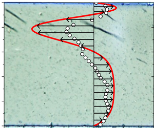
According to our observations, the rotating aggregates translate along the magnetic field gradient and are mostly accumulated behind the middle plane  $y\mathrm{\ \mathbin{\lower.3ex\hbox{$\buildrel> \over {\smash{\scriptstyle\sim}\vphantom{_x}}$}}\ }h/2$ of the channel, where the magnetic field is stronger (figure 2). In this § 4.1, we consider the motion of the whole colloid, which is characterized by the macroscopic quantities averaged over the whole volume of the colloid. Special attention must be paid to possible scale separation problems. As revealed in § 4.2, the average aggregate size is $L \times D = 30 \times 6$ μm, so that the size ratios of the aggregate size to the channel size are $L/h \approx 0.03{-}0.055$ and $D/b \approx 0.026$. In the studies of the fibre suspension rheology, it was established that the finite size of the fibres no longer affects the suspension viscosity or normal stresses at the ratios $L/h\mathrm{\ \mathbin{\lower.3ex\hbox{$\buildrel< \over {\smash{\scriptstyle\sim}\vphantom{_x}}$}}\ }0.2{-}0.33$ (Zirnsak, Hur & Boger Reference Zirnsak, Hur and Boger1994; Snook Reference Snook2015). Extrapolating these results to the present system, we expect that the colloid can still be considered as a continuous medium. The experimental time scale of the transient response related to the redistribution of aggregate concentration is much larger than the rotation period of aggregates. In this context, it is reasonable to consider the momentum balance equation averaged over the rotation period. Neglecting gravity, this equation takes the following general form valid for a suspension of elongated particles under magnetic field (Pokrovskiy Reference Pokrovskiy1978; Bashtovoi, Berkovsky & Vislovich Reference Bashtovoi, Berkovsky and Vislovich1988; López-López et al. Reference López-López, Kuzhir, Durán and Bossis2010):
 \begin{gather}\rho \left( {\frac{{\partial \boldsymbol{v}}}{{\partial t}} + (\boldsymbol{v}\boldsymbol{\cdot }\boldsymbol{\nabla })\boldsymbol{v}} \right) = \textrm{div}\,\boldsymbol{\sigma },\end{gather}
 \begin{gather}{\sigma _{ik}} ={-} P{\delta _{ik}} + 2{\eta _0}{\gamma _{ik}} + \sigma _{ik}^s + \sigma _{ik}^a + \sigma _{ik}^M,\end{gather}
 \begin{gather}\sigma _{ik}^M ={-} {\textstyle{1 \over 2}}{\mu _0}{H^2}{\delta _{ik}} + {H_i}{B_k},\end{gather}
 \begin{gather}\sigma _{ik}^a = {\textstyle{1 \over 2}}{\varepsilon _{ikl}}{K_l},\end{gather}
 \begin{gather}{K_l} = {\mu _0}{(\boldsymbol{M} \times \boldsymbol{H})_l},\end{gather}
where  $\rho $ is the colloid density; $\boldsymbol{v}$ and P are respectively the colloid velocity and pressure at a given point in the channel; ${\sigma _{ik}}$ are the components of the stress tensor $\boldsymbol{\sigma }$, with $\sigma _{ik}^s$ and $\sigma _{ik}^a$ being respectively symmetric and antisymmetric parts of the particle contribution to the viscous stress tensor, and $\sigma _{ik}^M$ being the Maxwell stress tensor; ${\gamma _{ik}} = (1/2)(\partial {v_i}/\partial {x_k} + \partial {v_k}/\partial {x_i})$ is the rate-of-strain tensor; ${\delta _{ik}}$ and ${\varepsilon _{ikl}}$ are Delta-Kronecker and Levi-Civita symbols, respectively; $\; {H_i}$ and $\; {B_k}$ are the i- or k-components of the magnetic field intensity vector $\boldsymbol{H}$ and magnetic flux density vector $\boldsymbol{B}$, respectively; $H = |\boldsymbol{H} |$; and ${K_l}$ is the l-component of the volume density $\boldsymbol{K}$ of a magnetic torque experienced by the magnetic colloid of a magnetization $\boldsymbol{M}$. The characteristic value of the particle stress $\sigma _{ik}^s$ is of the order of ${\sigma ^s}\sim \varPhi {r^2}{\eta _0}\dot{\gamma }$ with $\dot{\gamma }$ being a characteristic shear rate. In the dilute limit, $\varPhi {r^2} \ll 1$ valid for our experiments, the particle stress $\sigma _{ik}^s$ becomes negligible as compared with the solvent contribution, $2{\eta _0}{\gamma _{ik}}$, to the viscous stress, and is further omitted. With this in mind, and using the continuity equation, $\boldsymbol{\nabla }\boldsymbol{\cdot }\boldsymbol{v} = 0$, along with the magnetostatics Maxwell equations, $\boldsymbol{\nabla }\boldsymbol{\cdot }\boldsymbol{B} = 0$, $\boldsymbol{\nabla } \times \; \boldsymbol{H} = \boldsymbol{0}$, $\boldsymbol{B} = {\mu _0}(\boldsymbol{H} + \boldsymbol{M})$, the momentum balance equation (4.2a) becomes similar to that derived for the colloids of spherical magnetic particles (Bashtovoi et al. Reference Bashtovoi, Berkovsky and Vislovich1988):
 \begin{gather}\rho \left( {\frac{{\partial \boldsymbol{v}}}{{\partial t}} + (\boldsymbol{v}\boldsymbol{\cdot }\boldsymbol{\nabla })\boldsymbol{v}} \right) ={-} \boldsymbol{\nabla }P + {\eta _0}{\nabla ^2}\boldsymbol{v} + {\boldsymbol{F}_m},\end{gather}
 \begin{gather}{\boldsymbol{F}_m} = {\mu _0}(\boldsymbol{M}\boldsymbol{\cdot }\boldsymbol{\nabla })\boldsymbol{H} + {\textstyle{1 \over 2}}(\boldsymbol{\nabla } \times \boldsymbol{K}),\end{gather}
except for the viscosity  ${\eta _0}$ which is replaced by the viscosity of the whole colloid by Bashtovoi et al. (Reference Bashtovoi, Berkovsky and Vislovich1988), the difference coming from the dilute limit considered in the present work. In the last equation, ${\boldsymbol{F}_m}$ stands for the volume density of the magnetic force, whose expression can be simplified for our experimental conditions.
First, it is shown in Appendix C that in our experimental conditions (including linear magnetization limit and the ratio  ${L_H}/{L_\varPhi } \gg 1$ between the length scales of the magnetic and concentration field variations), the magnetic force density (4.3b) reduces to
 \begin{gather}{\boldsymbol{F}_m} \approx {\textstyle{1 \over 2}}\varPhi \varGamma {\mu _0}\boldsymbol{\nabla }({H^2}) + {\textstyle{1 \over 2}}(\boldsymbol{\nabla } \times \boldsymbol{K}),\end{gather}
where  $\varGamma $ is given by (C6b) in function of the phase lag $\theta $ and the magnetic susceptibility $\chi $ of aggregates.
Second, we suppose that a characteristic shear rate of the induced shear flow is much smaller than the rotational frequency of the aggregates,  $\dot{\gamma } \ll \omega $. This hypothesis, valid in the considered dilute regime, $\varPhi {r^2} \ll 1$, will be justified a posteriori once the velocity profile is calculated and the aggregate concentration determined (§ 4.5). With such a condition, the shear contribution to the hydrodynamic torque ${\boldsymbol{T}_h}$ experienced by an aggregate can be neglected and the torque balance in the inertialess limit will give us
 \begin{gather}\boldsymbol{K} \approx{-} n{\boldsymbol{T}_h} = 2{\eta _0}\beta \varPhi \boldsymbol{\omega },\end{gather}
with  $\boldsymbol{\omega }$ being a vector magnitude of the field angular frequency, $n = \varPhi /{V_a}$ being the number density of aggregates, each having a volume ${V_a}$ and $\beta $ is given by (4.1b).
Third, in the low-Reynolds-number limit, valid for our experiments, the convective term  $(\boldsymbol{v}\boldsymbol{\cdot }\boldsymbol{\nabla })\boldsymbol{v}$ can be neglected in the left-hand side of (4.3a). Finally, according to our observations, we consider only the steady-state regime at $t\mathrm{\ \mathbin{\lower.3ex\hbox{$\buildrel> \over {\smash{\scriptstyle\sim}\vphantom{_x}}$}}\ }100\;\textrm{s}$, meaning that the aggregate volume fraction $\varPhi $ and the fluid velocity $\boldsymbol{v}$ do not evolve with time. This last assumption will be revised in § 4.4 based on the results of the aggregate speed measurements. Applying the above conditions, (4.3) takes the following form:
 \begin{gather}- \boldsymbol{\nabla }P + {\eta _0}{\nabla ^2}\boldsymbol{v} + {\textstyle{1 \over 2}}\varPhi \varGamma {\mu _0}\boldsymbol{\nabla }({H^2}) + {\eta _0}\beta (\boldsymbol{\nabla }\varPhi \times \boldsymbol{\omega }) = {\bf 0}.\end{gather}
 Tracking back to our experimental geometry, we can provide further simplifications. First, the angular speed  $\boldsymbol{\omega }$ has the only non-zero $z$-component: ${\omega _z} ={-} \omega $ corresponding to the clockwise rotation in the $xy$-plane. Second, the channel length is much larger than two other dimensions, $l \gg b,h$ (figure 1), and considering the flow field far from the left and right borders of the channel, we can impose the single non-zero $x$-component of the velocity, ${v_x} = v(\kern0.7pt y,z)$ respecting the continuity equation, $\boldsymbol{\nabla }\boldsymbol{\cdot }\; \boldsymbol{v} = 0$. Third, in the experimental configuration of electromagnets, the $\boldsymbol{\nabla }({H^2})$ term has the only non-zero component along the y axis. Recall that the momentum balance equation is averaged over the aggregate rotation period, so that $\boldsymbol{\nabla }({H^2})$ term is given by the right-hand side of (2.3b).
These approximations allow us to rewrite (4.6) in the following component form:
 \begin{gather}\frac{{\partial P}}{{\partial x}} = {\eta _0}\left( {\frac{{{\partial^2}v}}{{\partial {y^2}}} + \frac{{{\partial^2}v}}{{\partial {z^2}}}} \right) - \beta {\eta _0}\omega \frac{{\partial \varPhi }}{{\partial y}},\end{gather}
 \begin{gather}\frac{{\partial P}}{{\partial y}} = \frac{1}{2}\varPhi \varGamma {\mu _0}\frac{{\partial {H^2}}}{{\partial y}} + \beta {\eta _0}\omega \frac{{\partial \varPhi }}{{\partial x}},\end{gather}
 \begin{gather}\frac{{\partial P}}{{\partial z}} = 0.\end{gather}
The image processing of our experimental snapshots (§ 3, Appendix B) shows that, once averaged over time, the aggregate concentration does not depend on x and on z coordinates. Thus, the last term in right-hand side of (4.7c) can be omitted. Since the term  $\partial {H^2}/\partial y$ is almost independent of $x,y,z$ in the present experimental conditions (cf. (2.3b)), integration of (4.7b), (4.7c) gives $P = \varPhi \varGamma {\mu _0}H_0^2y/(4{L_H}) + {\mathcal{G}}(x)$, where ${\mathcal{G}}(x)$ is an unknown function of x. With this in mind, the left-hand side of (4.7a), $\partial P/\partial x = \textrm{d}{\mathcal{G}}(x)/\textrm{d}\kern 0.06em x$ can only depend on x, while the right-hand side can only depend on y and z. With such a condition, (4.7a) can only hold if both its sides are independent of x, y and z, or rather $\partial P/\partial x = C$, with C being some unknown constant. Let us now introduce the following scaling factors for several physical magnitudes: $[v] = \beta \omega {\varPhi _0}h$ for the velocity, $[\varPhi ] = {\varPhi _0}$ – for the aggregate volume fraction and $[y] = h$, $[z] = b\;$ for the space coordinates, with ${\varPhi _0}$ being the average aggregate volume fraction in the suspension (before the aggregates migrate to the back region of the channel). The respective scaled quantities (hereinafter denoted by the tilde symbol) are obtained by dividing their dimensional counterparts by the scaling factors. Thus, (4.7a) can be rewritten in the following dimensionless form:
 \begin{gather}\frac{{{\partial ^2}\tilde{v}}}{{\partial {{\tilde{y}}^2}}} + {\gamma ^2}\frac{{{\partial ^2}\tilde{v}}}{{\partial {{\tilde{z}}^2}}} = 2{C_1} + \frac{{\partial \tilde{\varPhi }}}{{\partial \tilde{y}}},\end{gather}
 \begin{gather}\int_0^1 {\tilde{\varPhi }(\kern0.7pt \tilde{y})\,\textrm{d}\tilde{y}} = 1,\end{gather}
where  $\gamma = h/b$ and ${C_1} = Ch/(2\beta {\eta _0}\omega {\varPhi _0})$ is a dimensionless unknown constant having a meaning of the dimensionless pressure gradient. Equation (4.8b) is nothing but the particle conservation condition. Equation (4.8a) is subjected to the non-slip boundary condition and a condition of zero flow rate across the channel that should be respected for the considered closed channel:
 \begin{gather}\tilde{v}(0,\tilde{z}) = \tilde{v}(1,\tilde{z}) = \tilde{v}(\tilde{y},0) = \tilde{v}(\tilde{y},1) = 0,\end{gather}
 \begin{gather}\int_0^1 {\textrm{d}\tilde{z}} \int_0^1 {\tilde{v}(\tilde{y},\tilde{z})\,\textrm{d}\tilde{y}} = 0.\end{gather}
Analytical solution of the boundary value problem (4.8a), (4.9a), (4.9b) is obtained by the Fourier series expansion method similar to that originally used by Boussinesq in 1868 for calculations of the velocity profile in a rectangular duct – see for instance Cornish (Reference Cornish1928). Alternatively, noticing that (4.8a) has a mathematical structure of Poisson equation, the solution can be obtained by the Green function method. The final expression for the velocity profile in terms of infinite series reads
 \begin{gather}\tilde{v}(\tilde{y},\tilde{z}) = \sum\limits_{n = 1}^\infty {{D_n}{G_n}(\tilde{z})\,\textrm{sin}(n{\rm \pi} \tilde{y})} ,\end{gather}
 \begin{gather}{G_n}(\tilde{z}) = \frac{{\textrm{sinh}(n{\rm \pi} \tilde{z}/\gamma ) + \textrm{sinh}(n{\rm \pi} (1 - \tilde{z})/\gamma )}}{{\textrm{sinh}(n{\rm \pi} /\gamma )}} - 1,\end{gather}
 \begin{gather}{D_n} = \frac{{4[1 - {{( - 1)}^n}]}}{{{{(n{\rm \pi} )}^3}}}{C_1} - \frac{{2{K_n}}}{{n{\rm \pi} }},\end{gather}
 \begin{gather}{K_n} = \int_0^1 {\textrm{cos}(n{\rm \pi} \tilde{y})\tilde{\varPhi }(\kern0.7pt \tilde{y})\,\textrm{d}\tilde{y}} ,\end{gather}
 \begin{gather}{C_1} = \frac{1}{4}\frac{{\sum\limits_{n = 1}^\infty {{K_n}{M_n}[1 - {{( - 1)}^n}]/{{(n{\rm \pi} )}^2}} }}{{\sum\limits_{n = 1}^\infty {{M_n}[1 - {{( - 1)}^n}]/{{(n{\rm \pi} )}^4}} }},\end{gather}
 \begin{gather}{M_n} = 2\gamma \frac{{\textrm{tanh}[n{\rm \pi} /(2\gamma )]}}{{n{\rm \pi} }} - 1,\end{gather}
where analytical expressions for the coefficients  ${K_n}$ (4.10d) are provided in Appendix D based on the concentration profile $\tilde{\varPhi }(\kern0.7pt \tilde{y})$ determined experimentally in § 4.2 and theoretically in § 4.3.
The average dimensionless velocity across the channel thickness b is obtained by integration of (4.10a) over  $\tilde{z}$:
 \begin{gather}\langle \tilde{v}\rangle (\kern0.7pt \tilde{y}) = \int_0^1 {\tilde{v}(\tilde{y},\tilde{z})\,\textrm{d}\tilde{z}} = \sum\limits_{n = 1}^\infty {{D_n}{M_n}\,\textrm{sin}(n{\rm \pi} \tilde{y})} ,\end{gather}
with expressions for  ${D_n}$ and ${M_n}$ provided in (4.10c) and (4.10f), respectively.
Having obtained exact solution for the velocity profile, let us first analyse some limiting cases. First, in the case of homogeneous aggregate volume fraction  $\tilde{\varPhi }(\kern0.7pt \tilde{y}) = 1$ or $\varPhi = \textrm{const}\textrm{.} = {\varPhi _0}$, we obtain zero velocity everywhere in the channel. This result directly follows from (4.6), in which the last term on the right-hand side vanishes, and applying curl operator to the other three terms, one obtains $\boldsymbol{\nabla } \times ({\nabla ^2}\boldsymbol{v}) = {\bf 0}$ – a linear equation with a unique solution $\boldsymbol{v} = {\bf 0}$ satisfying the boundary conditions (4.9). This points to the necessity of a heterogeneous concentration profile ( $\boldsymbol{\nabla }\varPhi \ne {\bf 0}$) for generation of recirculation flows, in agreement with the basic claims of the present paper (cf. § 1), as also suggested in the literature on ferrofluid spin-up (Shliomis Reference Shliomis2021). Second, in a thick channel limit respecting the strong inequality $h \ll b \ll l$, the velocity is almost independent of the $\tilde{z}$ coordinate (except for the regions in a close proximity to the bottom and top channel walls, $\tilde{z} = 0\;\textrm{or}\;1$), and (4.10a), (4.11) reduce to
 \begin{gather}\tilde{v}(\kern0.7pt \tilde{y}) = \langle \tilde{v}\rangle (\kern0.7pt \tilde{y}) \approx {I_1}(\kern0.7pt \tilde{y}) + 3(2{I_2} - 1){\tilde{y}^2} + 2(1 - 3{I_2})\tilde{y},\quad \textrm{at}\;\gamma = h/b \ll 1,\end{gather}
 \begin{gather}{I_1}(\kern0.7pt \tilde{y}) = \int_0^{\tilde{y}} {\tilde{\varPhi }(\kern0.7pt \tilde{y})\,\textrm{d}\tilde{y}} ,\quad {I_2} = \int_0^1 {{I_1}(\kern0.7pt \tilde{y})\,\textrm{d}\tilde{y}} .\end{gather}
This approximate solution can be obtained by direct integration of (4.8a) neglecting the second term on the left-hand side.
Recall that dimensional flow velocity can be obtained by multiplying the dimensionless velocity ((4.10a) or (4.11)) by the scaling factor  $[v]$:
 \begin{gather}v(\kern0.7pt y,z) = \beta \omega {\varPhi _0}h\tilde{v}(\tilde{y},\tilde{z}),\end{gather}
 \begin{gather}\langle v\rangle (\kern0.7pt y) = \beta \omega {\varPhi _0}h\langle \tilde{v}\rangle (\kern0.7pt \tilde{y}),\end{gather}
with  $\tilde{y} = y/h$ and $\tilde{z} = z/b$.
Note that a similar scaling behaviour has been obtained by Bente et al. (Reference Bente, Bakenecker, von Gladiss, Bachmann, Cbers, Buzug and Faivre2021) for the velocity of the magnetic particle swarm under a coupled action of a rotating magnetic field and gravity. However, as mentioned in § 1, the results are obtained by considering zero tangential stress on the surface between the magnetic swarm and an ambient fluid, so that existence of such net surface seems to be necessary (at least from theoretical perspective) to generate the swarm motion. Such a surface is absent in our present study.
To get numerical values of the velocity, we need to define the factor  $\beta $ depending on the aggregate aspect ratio r (4.1b), the average aggregate volume fraction ${\varPhi _0}$, as well as the aggregate concentration profile $\tilde{\varPhi }(\kern0.7pt \tilde{y})$ intervening into (4.10d). In the present study, the first two quantities ( $\beta $ and ${\varPhi _0}$) are drawn from the experiments, while the concentration profile is both measured (§ 4.2) and evaluated by hydrodynamic diffusion approach (§ 4.3).
4.2. Aggregate size and concentration profile: experiments
The experimental distribution of aggregate lengths L, obtained through image processing as detailed in § 2, is shown in figure 3(a) for the following set of experimental parameters: f = 5 Hz, H 0 = 6.4 kA m−1, h = 1000 μm,  ${\varphi _p} = 1.6 \times {10^{ - 3}}$. The distributions of aggregate diameters D and β parameters (4.1b) were also measured. The average value and standard deviation for these three quantities is equal to $L = 30 \pm 6\;{\rm \mu}\textrm{m}$, $D = 6 \pm 1\;{\rm \mu}\textrm{m}$ and $\beta = 14 \pm 2$. Surprisingly, these quantities remained unchanged (within the experimental errors) in the range of our experimental parameters f = 5–15 Hz, H 0 = 3–9.5 kA m−1, h = 550–1000 μm, ${\varphi _p} = (1.6{-}3.2) \times {10^{ - 3}}$. This is in contradiction to the theoretical models (Melle & Martin Reference Melle and Martin2003; Raboisson-Michel et al. Reference Raboisson-Michel, Queiros Campos, Schaub, Zubarev, Verger-Dubois and Kuzhir2020) predicting hydrodynamic rupture of aggregates leading to a decrease of their aspect ratio according to the scaling law $r \propto {\omega ^{ - 1/2}}$. However, in our previous experiments with homogeneous rotating magnetic field, we have already observed a very small variation of the aggregate length with the field frequency (cf. figure 6 of Raboisson-Michel et al. Reference Raboisson-Michel, Queiros Campos, Schaub, Zubarev, Verger-Dubois and Kuzhir2020). Such an effect can be tentatively explained by thermodynamic arguments, but first, we need to clearly define different volume fractions involved in the further analysis.

Figure 3. (a) Experimental histograms of the aggregate length distribution. (b) Experimental and calculated profiles of the aggregate volume fraction across the channel y-dimension. Both graphs correspond to the following set of experimental parameters: f = 5 Hz, H 0 = 6.4 kA m−1, h = 1000 μm,  ${\varphi _p} = 1.6 \times {10^{ - 3}}.$
The volume fraction of individual nanoparticles (without adsorbed sodium citrate layer) is denoted by  ${\varphi _p}$ and is a well-defined quantity in our colloids ( ${\varphi _p} = (1.6{-}3.2) \times {10^{ - 3}}$). As mentioned in § 2, the individual nanoparticles are assembled into primary aggregates due to weakly attractive colloidal interactions in the absence of the magnetic field. However, only a small fraction of individual nanoparticles forms these aggregates, as revealed by hydrodynamic size distribution measurements. The volume fraction of primary aggregates ${\varphi _0}$ is defined as the volume occupied by the primary aggregates divided by the colloid volume. This quantity cannot be easily measured in experiments. It is supposed to vary linearly with the volume fraction ${\varphi _p}$ of individual nanoparticles. When the magnetic field is applied, the primary aggregates are self-assembled into the elongated secondary aggregates. Again, only a fraction of the primary aggregates forms the secondary ones. The remaining number of primary aggregates is characterized by the volume fraction $\varphi $, which decreases with time.
Tracking back to the explanation of the aggregate length independence of f, H 0, h,  ${\varphi _p}$, we notice that there exist two limitations for the aggregate maximal volume. On one hand, in the absence of the aggregate growth by absorption of neighbouring nanoparticles by the field-induced aggregates, the maximal aggregate volume is limited by hydrodynamic forces coming from either flow fields of neighbouring aggregates or short-ranged hydrodynamic interactions at collisions with neighbouring aggregates. This volume is expected to scale as ${V_{max1}} \propto {D^3}{[{\mu _0}{H^2}/({\eta _0}\omega )]^{1/2}}$ (Raboisson-Michel et al. Reference Raboisson-Michel, Queiros Campos, Schaub, Zubarev, Verger-Dubois and Kuzhir2020). On the other hand, in the absence of coalescence/fragmentation, the aggregate growth stops when the supersaturation $\varDelta = \varphi - \varphi ^{\prime}$ of the colloid (excess concentration of primary aggregates $\varphi $ with respect to the concentration at the aggregation threshold $\; \varphi ^{\prime}$) goes to zero. This corresponds to the maximal aggregate volume (Raboisson-Michel et al. Reference Raboisson-Michel, Queiros Campos, Schaub, Zubarev, Verger-Dubois and Kuzhir2020): ${V_{max2}} = {\varDelta _0}/(\varphi ^{\prime\prime}n)$, where $\varphi ^{\prime\prime} \approx \textrm{const}\textrm{.} \approx 0.3$ is the nanoparticle concentration inside the aggregates, n is the number density of the secondary aggregates and ${\varDelta _0 = {\varphi _0} - \varphi ^{\prime}}$ is the initial supersaturation of primary aggregates. The ${V_{max2}}$ value could be nearly independent of the parameters $\omega $, H and ${\varphi _p}$ provided that the initial supersaturation ${\varDelta _0}$ is independent of $\omega $ (Raboisson-Michel et al. Reference Raboisson-Michel, Queiros Campos, Schaub, Zubarev, Verger-Dubois and Kuzhir2020), and assuming that the number density n is linear with ${\varphi _0}$ (and ${\varphi _p}$), and at small aggregation threshold, $\varphi ^{\prime} \ll {\varphi _0}$, the ratio ${\varDelta _0}/n$ is nearly independent of ${\varphi _0}$ ( ${\varphi _p}$) and H. In the present situation, when both aggregate growth, coalescence and fragmentation are observed, the final aggregate volume is expected to be situated between ${V_{max1}}$ and ${V_{max2}}$. It is possible that in our experimental conditions, the maximal aggregate volume is closer to the ${V_{max2}}$ value, which is independent of $\omega $, H, ${\varphi _p}$ and h parameters. To get a grounded confirmation of this scenario, we need to reconsider the kinetics of field-induced phase assembly under rotating fields accounting for growth, coalescence and fragmentation events.
The experimental average value of the aggregate volume fraction is evaluated to be  ${\varPhi _0} = (4.0 \pm 1.0) \times {10^{ - 4}}$ for ${\varphi _p} = 1.6 \times {10^{ - 3}}$ and ${\varPhi _0} = (6.5 \pm 2.3) \times {10^{ - 4}}$ for ${\varphi _p = 3.2 \times 10^{ - 3}}$ independently of the field frequency $\omega $, amplitude H and channel height h. High statistical errors of ${\varPhi _0}$ do not allow precise determination of the effect of nanoparticle concentration ${\varphi _p}$ on the concentration of the secondary aggregates ${\varPhi _0}$. However, we can discern a global tendency of increasing ${\varPhi _0}$ with increasing ${\varphi _p}$. Qualitatively, this behaviour is consistent with the above evaluation of the maximal volume ${V_{max2}}$ and of the initial supersaturation ${\varDelta _0} = {\varphi _0} - \varphi ^{\prime} \approx {\varphi _0}$ resulting in ${\varPhi _0} = n{V_{max2}} \approx {\varphi _0}/\varphi ^{\prime\prime}$. The ensemble of the experimental values determined in this section are summarized in table 1 along with their standard deviations.
The experimental aggregate concentration profile  $\varPhi (\kern0.7pt y)$ across the channel was obtained through image processing (§ 2, Appendix B) and it was normalized by the average value ${\varPhi _0}$, namely $\tilde{\varPhi }(\kern0.7pt \tilde{y}) = \varPhi (\kern0.7pt y = \tilde{y}h)/{\varPhi _0}$. The experimental profile $\tilde{\varPhi }(\kern0.7pt \tilde{y})$ is represented by dots in figure 3(b), while the error bars correspond to the standard deviation between six measurement series. As observed on the snapshot of figure 2, the concentration profile is non-uniform: the aggregate volume fraction remains near zero in the front part of the channel at $\tilde{y}\mathrm{\ \mathbin{\lower.3ex\hbox{$\buildrel< \over {\smash{\scriptstyle\sim}\vphantom{_x}}$}}\ }0.6$; it shows an abrupt increase at $0.6\mathrm{\ \mathbin{\lower.3ex\hbox{$\buildrel< \over {\smash{\scriptstyle\sim}\vphantom{_x}}$}}\ }\tilde{y}\mathrm{\ \mathbin{\lower.3ex\hbox{$\buildrel< \over {\smash{\scriptstyle\sim}\vphantom{_x}}$}}\ }0.9$ followed by a decrease near the back wall at $0.9\mathrm{\ \mathbin{\lower.3ex\hbox{$\buildrel< \over {\smash{\scriptstyle\sim}\vphantom{_x}}$}}\ }\tilde{y} \le 1$. This last decrease is related to geometrical constraints. In fact, when spinning under a rotating field, the aggregates cannot penetrate the back wall, so that the distance between their geometrical centres and the back wall cannot be smaller than the aggregate half-length. This creates a kind of depletion layer near the back wall with a smaller aggregate volume fraction. For calculations of the velocity profile, we fitted the experimental concentration profile with a Gaussian function (red solid line in figure 3b), as follows:
 \begin{gather}\tilde{\varPhi }(\kern0.7pt \tilde{y}) = A\,\textrm{exp}\left( { - \frac{{{{(\tilde{y} - {{\tilde{y}}_0})}^2}}}{{{{(2\delta )}^2}}}} \right),\end{gather}
 \begin{gather}A = {\left[ {\delta \sqrt {\rm \pi}\left( {\textrm{erf}\left( {\frac{{1 - {{\tilde{y}}_0}}}{{2\delta }}} \right) + \textrm{erf}\left( {\frac{{{{\tilde{y}}_0}}}{{2\delta }}} \right)} \right)} \right]^{ - 1}},\end{gather}
where  $\textrm{erf(} \ldots )$ stands for the error function; the value of the normalization constant A is chosen to respect the particle conservation condition (4.8b); and the fitting parameters ${\tilde{y}_0} = 0.9$ and $\delta = 0.07$ (reported in table 1) represent the position of the Gaussian peak and the distribution width, respectively. Note finally that the Gaussian fit (4.14) allows evaluation of the experimental length-scale of the concentration variation: ${L_\varPhi } = \sqrt 2 \delta h \approx 100\;{\rm \mu}\textrm{m}$ for the channel width $h = 1000\;{\rm \mu}\textrm{m}$.
4.3. Aggregate concentration profile: hydrodynamic diffusion model
Let us now try to evaluate the concentration profile independently from experimental data. From the first glance, this profile comes from the balance between the magnetic force pushing the aggregates toward the back wall and hydrodynamic interaction repulsing the aggregates from the back wall that have been extensively studied by different authors (see for example Hsu & Ganatos Reference Hsu and Ganatos1994; Mitchell & Spagnolie Reference Mitchell and Spagnolie2015; Zheng et al. Reference Zheng, Xu, Wang and Han2022). The aggregate position y can be evaluated by balancing both these forces. Using the full hydrodynamic resistance matrix of an ellipsoid translating and spinning along a solid wall (calculated by boundary integral method by Hsu & Ganatos (Reference Hsu and Ganatos1989, Reference Hsu and Ganatos1994)), we evaluate that the extremity of the aggregates (when they are oriented normal to the back wall) is separated from the back wall by a small distance  ${h_w} \ll L$, recalling that $L \approx 30$ μm is the average aggregate length. This means that we should find all the aggregates confined near the back wall within a thin layer of a thickness ${\sim} L$ taking 3 % of the channel width. This is not consistent with the measured concentration profile which spreads over a 400 μm thick layer taking approximately 40 % of the channel width ( $0.6\mathrm{\ \mathbin{\lower.3ex\hbox{$\buildrel< \over {\smash{\scriptstyle\sim}\vphantom{_x}}$}}\ }\tilde{y} \le 1$, cf. figure 3b). Such a discrepancy cannot be explained by the polydispersity of the aggregate length because the number of aggregates of the length $L > 100$ μm is only approximately 3 % (figure 3a). However, it is often observed in experiments that the geometric centre of an aggregate gets spinning around a neighbouring larger aggregate, as already mentioned in § 3. This overall motion of the aggregates can be imagined as a combination of a regular leftward translation along the back wall and a stochastic reciprocal translation in the x and y directions, as a result of hydrodynamic interactions with neighbouring aggregates. The stochastic part of this motion is responsible for spreading of the aggregate positions across the channel, leading to spreading of the concentration profile. It is thus convenient to mimic this process by hydrodynamic diffusion, as often suggested for colliding spherical particles in concentrated suspensions (see for instance Nicolai et al. (Reference Nicolai, Herzhaft, Hinch, Oger and Guazzelli1995)). The hydrodynamic diffusion has also been suggested in the mathematical model of magnetically assisted delivery of thrombolytics (Clements Reference Clements2016). However, the nature of this diffusion was not specified, and the diffusivity was not evaluated, which may have biased conclusions on the aggregate angular speed effect on generated macroscopic flow.
In the present case, the associated translational diffusivity can be evaluated through the mean free path approach applied to two-dimensional motion of aggregates (Pitaevskii & Lifshitz Reference Pitaevskii and Lifshitz2012):  $\mathfrak{D} = (1/2)U\lambda $, where U is the average velocity of stochastic motion and $\lambda $ is the mean free path. In our case, the trajectory of the aggregate centre changes each time when the target aggregate is ‘trapped’ into the vortex flow field of a neighbouring aggregate and starts spinning around the latter. Thus, the mean free path $\lambda $ is a distance the target aggregate travels from the moment it is ‘left free’ from one aggregate and ‘trapped’ by another aggregate. Our observations show that in the back part of the channel, the large aggregates are situated close to each other and the small aggregates spin around the large ones (of a length $L$) with a linear velocity $U \approx \omega L/2$ traveling a distance $\lambda \sim L$ between two large aggregates. This results to the following scaling for the diffusivity:
 \begin{gather}\mathfrak{D} = \frac{{\omega {L^2}}}{{4{C_2}}},\end{gather}
where the average aggregate length can be chosen for the characteristic length L and  ${C_2}$ is an unknown constant supposed to be of the order of unity and intentionally introduced into the denominator for further utility.
We need now to write down the mass conservation and momentum equations for the solid phase (field-induced aggregates) of the colloid using the general framework of Drew & Lahey (Reference Drew and Lahey1993), Nott & Brady (Reference Nott and Brady1994) and Morris & Boulay (Reference Morris and Boulay1999) applied to the inertialess limit and incorporating hydrodynamic diffusion:
 \begin{gather}\frac{{\partial \varPhi }}{{\partial t}} + \boldsymbol{\nabla }\boldsymbol{\cdot }\boldsymbol{j} = 0,\end{gather}
 \begin{gather}\boldsymbol{j} = \varPhi \boldsymbol{u} - \mathfrak{D}\boldsymbol{\nabla }\varPhi ,\end{gather}
 \begin{gather}{\bf 0} = \boldsymbol{\nabla }\boldsymbol{\cdot }{\boldsymbol{\sigma }^s} + n{\boldsymbol{F}_h} + {\boldsymbol{F}_m},\end{gather}
where  $\boldsymbol{j}$ is the volume flux density of aggregates, $\boldsymbol{u}$ is the average migration velocity of the aggregates, n is their number fraction, ${\boldsymbol{\sigma }^s}$ is the symmetric part to the particle contribution to the viscous stress tensor, ${\boldsymbol{F}_h}$ is the hydrodynamic drag force that the suspending liquid exerts on the aggregates, and ${\boldsymbol{F}_m}$ is the magnetic body force averaged over the whole suspension volume and provided by (4.4). The term $\boldsymbol{\nabla }\boldsymbol{\cdot }{\boldsymbol{\sigma }^s}$ has already been shown negligible with respect to ${\eta _0}{\nabla ^2}\boldsymbol{v}$, and since ${\eta _0}{\nabla ^2}\boldsymbol{v}$ is of the same order of magnitude as ${\boldsymbol{F}_m}$ (cf. (4.3a)), the term $\boldsymbol{\nabla }\boldsymbol{\cdot }{\boldsymbol{\sigma }^s}$ can also be omitted in (4.16b). As already stated, the hydrodynamic interactions between aggregates and the back wall cannot solely provide a correct estimation of the concentration profile. Moreover, tracking of aggregate angular motion with a high-speed camera shows that the aggregate angular speed does not change (within experimental precision) during the rotation period and is always equal to the field angular frequency, even for the aggregates whose end passes very close to the channel wall. This is possibly a consequence of the low Mason number $Ma \ll 1$ (table 1) depreciating hydrodynamic interactions even in close proximity to the wall. So, we can suppose that the wall interaction is at least not decisive in the current problem. In this context, as a first approximation, we can use an expression for the hydrodynamic drag force for the aggregates in an unbounded liquid neglecting wall interactions: ${\boldsymbol{F}_h} ={-} \boldsymbol{\xi }\boldsymbol{\cdot }(\boldsymbol{u} - \boldsymbol{v})$, where $\boldsymbol{\xi }$ is the tensor of hydrodynamic friction coefficients of aggregates and $\boldsymbol{v}$ is the suspension velocity defined by the momentum equation (4.3a). Equations can be further simplified if we recall that the concentration profile is steady state and all the physical magnitudes are independent of x. This leads us to ${j_x} = 0$, $\textrm{d}{j_y}/\textrm{d}y = 0$ in (4.16a), and with non-penetration condition at the front and back walls, we get zero aggregate flux across the channel:
 \begin{gather}{j_y} = \varPhi {u_y} - \mathfrak{D}\frac{{\textrm{d}\varPhi }}{{\textrm{d}y}} = 0.\end{gather}
 Combining (4.4) and (4.16c), we get the expression for the aggregate migration speed  $\boldsymbol{u}$ and its y component ${u_y}$:
 \begin{gather}\boldsymbol{u} = \boldsymbol{v} + \boldsymbol{b}\boldsymbol{\cdot }{\boldsymbol{F}_m},\end{gather}
 \begin{gather}{u_y} = {v_y} - \frac{{{b_{yx}}}}{n}\beta {\eta _0}\omega \frac{{\textrm{d}\varPhi }}{{\textrm{d}y}} + {b_{yy}}\frac{1}{2}{V_a}\varGamma {\mu _0}\frac{{\partial {H^2}}}{{\partial y}},\end{gather}
where  ${V_a} = {\rm \pi}{D^2}L/6$ is the aggregate volume, $\boldsymbol{b}$ is the hydrodynamic mobility tensor with the components ${b_{yx}} = ({b_\parallel } - {b_ \bot })\,\textrm{cos}(\omega t - \theta )\,\textrm{sin}(\omega t - \theta )$, $\; {b_{yy}} = {b_\parallel }\,\textrm{co}{\textrm{s}^2}(\omega t - \theta ) + {b_ \bot }\,\textrm{si}{\textrm{n}^2}(\omega t - \theta )$ expressed through the mobilities ${b_\parallel }$, ${b_ \bot }$ parallel and perpendicular to the aggregate major axis. The last magnitudes are evaluated in high aspect ratio limit $r \gg 1$ (Brenner Reference Brenner1974):
 \begin{gather}{b_{{\parallel} , \bot }} = \frac{2}{{{\eta _0}L{\xi _{{\parallel} , \bot }}}},\quad {\xi _\parallel } = \frac{{4{\rm \pi} }}{{\textrm{ln}(2r) - 1/2}},\quad {\xi _ \bot } = \frac{{8{\rm \pi} }}{{\textrm{ln}(2r) + 1/2}}.\end{gather}
Equation (4.18) still represents instantaneous value of the migration speed, provided that the expression (4.4) is valid not only for time-averaged value of  ${\boldsymbol{F}_m}$ but also for its instantaneous value with the field gradient $\partial {H^2}/\partial y$ given by (2.3a). However, the first term in (4.18a) vanishes because the y component ${v_y}$ of the instantaneous velocity field of the whole colloid is zero thanks to the inertialess limit and specific boundary conditions ((4.9a), (4.9b)). In addition, averaging of (4.18b) over the rotation period of the aggregates cancels the second term on the right-hand side and finally gives
 \begin{gather}{u_y} = {\rm \pi}\varGamma \psi \frac{{{\mu _0}H_0^2{D^2}}}{{48{\eta _0}{L_H}}},\end{gather}
 \begin{gather}\psi = \frac{{2 + \textrm{cos(}2\theta )}}{{{\xi _\parallel }}} + \frac{{2 - \textrm{cos(}2\theta )}}{{{\xi _ \bot }}},\end{gather}
where  $\varGamma $ is given by (C6b) and the length scale ${L_H} \approx 27\;\textrm{mm}$ of the magnetic field variation was defined in § 2 (cf. (2.2)). Substituting (4.20a) into (4.17) and integrating, we get the following expression for the concentration profile:
 \begin{gather}\tilde{\varPhi }(\kern0.7pt \tilde{y}) = {C_3}\,\textrm{exp}(\alpha \tilde{y}),\end{gather}
 \begin{gather}\alpha = \frac{{{u_y}h}}{\mathfrak{D}} = {C_2}{\rm \pi} \varGamma \psi \frac{{{\mu _0}H_0^2h}}{{12{\eta _0}\omega {r^2}{L_H}}},\end{gather}
where  ${C_3}$ is an integration constant.
We can see that (4.21) simply reflects Boltzmann statistical distribution corresponding to the balance between diffusive and magnetophoretic fluxes. As a consequence, it gives a monotonous increase of the aggregate concentration across the channel with the maximal concentration on the channel back wall. In reality, the geometric centres of the aggregates cannot approach the back channel wall to a distance closer than their half-length. Thus, as already stated in § 4.2, we expect a depletion layer poor of aggregates near the back wall. However, due to polydispersity of the aggregate length, abrupt changes of the aggregate concentration across the depletion layer are not expected. The characteristic thickness of this layer  ${L_d}$ is possibly defined by the length of the largest aggregates and can be taken as an adjustable parameter. A similar depletion layer (not allowing the aggregates to cross the wall) should in principle exist near the front wall. For the sake of simplicity, we can suppose that the concentration profile linearly decreases to zero within both depletion layers and is given by (4.21a) outside these layers:
 \begin{gather}\tilde{\varPhi
}(\kern0.7pt \tilde{y}) = {C_3} \times \left\{
{\begin{array}{@{}ll@{}} \dfrac{{\textrm{exp}(\alpha \kappa
)}}{\kappa }\tilde{y},& \textrm{at}\;0 \le \tilde{y} <
\kappa ,\\
\textrm{exp}(\alpha \tilde{y}),& \textrm{at}\;\kappa \le \tilde{y} < 1 - \kappa, \\
\dfrac{{\textrm{exp}(\alpha (1 - \kappa ))}}{\kappa }(1 -
\tilde{y}),& \textrm{at}\;1 - \kappa < \tilde{y} \le 1,
\end{array}} \right.\end{gather}
\begin{gather}\tilde{\varPhi
}(\kern0.7pt \tilde{y}) = {C_3} \times \left\{
{\begin{array}{@{}ll@{}} \dfrac{{\textrm{exp}(\alpha \kappa
)}}{\kappa }\tilde{y},& \textrm{at}\;0 \le \tilde{y} <
\kappa ,\\
\textrm{exp}(\alpha \tilde{y}),& \textrm{at}\;\kappa \le \tilde{y} < 1 - \kappa, \\
\dfrac{{\textrm{exp}(\alpha (1 - \kappa ))}}{\kappa }(1 -
\tilde{y}),& \textrm{at}\;1 - \kappa < \tilde{y} \le 1,
\end{array}} \right.\end{gather} \begin{gather}{C_3} = {\left[ {\textrm{exp}(\alpha \kappa )\left( {\frac{\kappa }{2} - \frac{1}{\alpha }} \right) + \textrm{exp}(\alpha (1 - \kappa ))\left( {\frac{\kappa }{2} + \frac{1}{\alpha }} \right)} \right]^{ - 1}},\end{gather}
where  $\kappa = {L_d}/h$ and we have used the aggregate conservation condition (4.8b) to get the expression for the constant ${C_3}$. The upper, middle and lower expressions of (4.22a) stand for the front depletion layer, the main middle layer of the channel and the back depletion layer, respectively.
The experimental concentration profile was fitted by (4.22a). The fitted curve is presented by a blue solid line in figure 3(b). We observe a rather good agreement between experiments and theory at reasonable values of the adjustable parameters:  ${C_2} = 0.81$ ( ${C_2} = O(1)$ was expected) and ${L_d} = 100\;{\rm \mu}\textrm{m}$, resulting in $\kappa = 0.1$, which corresponds to the tail of the aggregate length distribution (figure 3a). The sharp peak at $\tilde{y} = 1 - \kappa = 0.9$ of the theoretical concentration profile comes from the depletion layer approximation imposing an abrupt change of the exponentially growing concentration outside the layer to linearly decreasing concentration inside the layer. However, such a sharp profile is not shocking and seems to be well compared to the experimental shape. Furthermore, (4.21a), (4.21b) allow us to define the expression for the length scale of the concentration variation:
 \begin{gather}{L_\varPhi } = \frac{h}{\alpha } = \frac{{12{\eta _0}\omega {r^2}}}{{{C_2}{\rm \pi} \varGamma \psi {\mu _0}H_0^2}}{L_H} \approx \frac{{36}}{{7{C_2}}}{L_H}Ma\sim {L_H}Ma,\end{gather}
where the Masson number is defined by (4.1a), and the pre-factor  $36/(7{C_2}) = O(1)$ is a result of the approximations $r \gg 1$, $\chi \gg 1$ and $\theta ,Ma \ll 1$. Note that the later strong inequality allows using the values of $\varGamma $ and $\psi $ parameters ((C6b) and (4.20b)) at $\theta = 0$, namely
 \begin{gather}\varGamma \approx \chi ,\psi \approx \frac{3}{{{\xi _\parallel }}} + \frac{1}{{{\xi _ \bot }}}\quad \textrm{at}\;Ma,\;\theta \ll 1.\end{gather}
At the given magnetic field frequency and amplitude, f = 5 Hz, H 0 = 6.4 kA m−1, the Mason number is  $Ma \approx 1.1 \times {10^{ - 3}}$, so with ${L_H} \approx 27\;\textrm{mm}$, we get ${L_\varPhi } \approx 190\;{\rm \mu}\textrm{m}$, which is consistent with the measured concentration profile (figure 3b) and with experimentally evaluated length scale ${L_\varPhi } \approx 100\;{\rm \mu}\textrm{m}$ (§ 4.2). Anyway, both experimental and theoretical evaluation of the concentration variation length scale clearly show that it is much lower than the field variation length scale, ${L_\varPhi } \ll {L_H}$, which is the consequence of the low-Mason-number limit $Ma \ll 1$, as inferred from (4.23). Recall that such scale separation is important for simplification of the magnetic force expression to (4.4) (cf. Appendix C).
4.4. Velocity profiles: experiments and comparison with the theory
Let us now focus on the velocity profiles of the recirculation flow in the closed microchannel, recalling that experimental and theoretical profiles describe the effective velocities of the whole colloid without a distinguishing of aggregate motion from the suspending fluid motion. An example of the velocity vector field obtained experimentally from the PIV analysis for a moment of time  $t = 60\;\textrm{s}$ elapsed from the moment of the magnetic field application is shown in figure 4. It is clear from this figure that the velocity field is in general strongly perturbed by the presence of rotating aggregates. One clearly observes clockwise flow vortexes within the area swapped by the aggregate clockwise rotation. Interference between the vortexes created by neighbouring aggregates gives a rather complicated flow pattern. However, one clearly distinguishes a regular rightward flow in the channel's front layer free of aggregates. As already discussed in § 3, this rightward flow arises to compensate the leftward one induced by the aggregate translation along the back wall.

Figure 4. Velocity vector field deduced from the PIV analysis taken at a moment of time  $\; t = 60\;\textrm{s}$ and for the following set of experimental parameters: f = 5 Hz, H = 6.4 kA m−1, h = 1000 μm, ${\varphi _p} = 1.6 \times {10^{ - 3}}$. The coloured arrows stand for the velocity vectors whose x and y components enter (green arrows) the $10 \times 5$ px frame−1 window (cf. Appendix A) or lie outside this window (brown arrows). White thin rods stand for the position of aggregates, within which the instantaneous velocity profile cannot be established.
To smooth the effects of the flow irregularities introduced by rotating aggregates, the longitudinal ( $x$-) component of the velocity profiles was averaged over either the observation window length l or observation period T, with the respective average magnitudes ${\langle {v_x}(\kern0.7pt y,t)\rangle _l}$ or ${\langle {v_x}(x,y)\rangle _T}$, defined in Appendix A, with the time t being counted from the beginning of the steady-state regime, thus 100 s after the moment of the magnetic field application. The experimental colourmaps of the ${\langle {v_x}(\kern0.7pt y,t)\rangle _l}$- and ${\langle {v_x}(x,y)\rangle _T}$-dependencies are shown in figure 5(a,b), respectively. First, we clearly observe a recirculation flow in both these figures: the back layer (upper half of the colourmaps) exhibits the leftward flow with negative longitudinal speeds and the front layer (lower half of the colourmaps) shows a rightward flow with positive speeds. Second, a few white-coloured vertical bands sometimes appear in the spatiotemporal colourmap ${\langle {v_x}(\kern0.7pt y,t)\rangle _l}$ (figure 5a). These bands correspond to near zero velocity and point out a go-and-stop (or rather fast and slow) sequence of the recirculation flow. This sequence visually corresponds to the fluctuation of the aggregate amount (or rather instantaneous volume fraction ${\varPhi _0}(t)$) in the observation window: smaller ${\varPhi _0}$ results in slower recirculation, higher ${\varPhi _0}$ results in stronger flows, in agreement with (4.13). However, excluding these fluctuations from consideration, we can claim that the steady-state velocity profile globally holds for the whole analysed period of 200 s starting from the beginning of the steady-state regime until the end of the experiment. Third, the spatial colourmap ${\langle {v_x}(x,y)\rangle _T}$ in figure 5(b) shows that the velocity field averaged over time is globally independent of the longitudinal coordinate with some fluctuations likely appearing as a result of a relatively small number of aggregates per observation window increasing the dispersion of the statistical averaging. An independence of the velocity profile on x is likely ensured thanks to the fact that the observation window is centred with respect to the channel centre and it is a few times shorter than the channel full length, such that the fringing effects from the left and the right borders of the channel are not perceived.

Figure 5. (a) Spatiotemporal  ${\langle {v_x}(\kern0.7pt y,t)\rangle _l}$ and (b) 2-D spatial ${\langle {v_x}(x,y)\rangle _T}$ experimental velocity maps averaged over one of six movies for the following set of experimental parameters: f = 5 Hz, H = 6.4 kA m−1, h = 1000 μm, ${\varphi _p} = 1.6 \times {10^{ - 3}}$. The red and blue colours stand respectively for the rightward and leftward flows.
Finally, let us consider the velocity profiles  ${\langle {v_x}(\kern0.7pt y)\rangle _{l,T}} \equiv \langle v\rangle (\kern0.7pt y)$ averaged over time and length of the observation window, as detailed in Appendix A. Such averaging allows smoothing longitudinal and temporal fluctuations, and focusing on the net effect of the rotating magnetic field on generated recirculation flows. The experimental averaged velocity profiles $\langle v\rangle (\kern0.7pt y)$ are compared with the calculated profiles in figure 6 using either Gaussian fit of the experimental concentration field ((4.14), figure 6a) or theoretical concentration field evaluated through hydrodynamic diffusion approach ((4.22), figure 6b). Analytical expressions for the coefficients ${K_n}$ (4.10d) intervening into the velocity profile (4.10a) are provided in Appendix D for both cases of the concentration profiles. Points correspond to the data averaged over six experimental runs. Solid lines correspond to the upper and the lower limits of the calculated profile which were obtained as ${v_{up}} = v(1 + \varepsilon )$ and ${v_{low}} = v(1 - \varepsilon )$, where $v = \langle v\rangle (\kern0.7pt y)$ is the velocity profile calculated using (4.11), (4.13b) using the average experimental values of $\beta ,\;{\varPhi _0},\;h$, and $\varepsilon \approx {({(\Delta \beta /\beta )^2} + {(\Delta {\varPhi _0}/{\varPhi _0})^2} + {(\Delta h/h)^2})^{1/2}}$ is the relative velocity error evaluated using experimental standard deviations $\Delta \beta ,\;\Delta {\varPhi _0},\;\Delta h$ of $\beta ,\;{\varPhi _0},\;h$ (cf. table 1).

Figure 6. Experimental (symbols with error bars) and theoretical (solid lines) velocity profiles  ${\langle {v_x}(\kern0.7pt \tilde{y})\rangle _{l,T}} \equiv \langle v\rangle (\kern0.7pt \tilde{y})$ averaged over time and length of the observation window and presented for the following set of experimental parameters: f = 5 Hz, H = 6.4 kA m−1, h = 1000 μm, ${\varphi _p} = 1.6 \times {10^{ - 3}}$. The calculated velocity profiles correspond to either (a) Gaussian fit of the concentration profile (4.14) or (b) the concentration profile evaluated by the hydrodynamic diffusion approach (4.22). The shaded regions in panels (a) and (b) encompass the region of the model validity.
As inferred from this figure, both experimental and theoretical velocity profiles reflect recirculation flows. In the close vicinity to the back wall,  $0.9\mathrm{\ \mathbin{\lower.3ex\hbox{$\buildrel< \over {\smash{\scriptstyle\sim}\vphantom{_x}}$}}\ }\tilde{y} < 1$, a distinguishable rightward flow is observed in experiments and confirmed by the model. This flow is likely associated to the propulsion of the fluid layer to the right along the wall by the upper end of the aggregates spinning in the clockwise direction. In the region still situated in the back part of the channel but further from the wall, $0.5\mathrm{\ \mathbin{\lower.3ex\hbox{$\buildrel< \over {\smash{\scriptstyle\sim}\vphantom{_x}}$}}\ }\tilde{y}\mathrm{\ \mathbin{\lower.3ex\hbox{$\buildrel< \over {\smash{\scriptstyle\sim}\vphantom{_x}}$}}\ }0.9$, a leftward intense flow is observed and could be assigned to the propulsion of the liquid layer to the left by lower ends of the aggregates. The flux generated by the upper ends of the aggregates is smaller because of the proximity with the wall imposing non-slip condition. The front layer of the channel, $0 < \tilde{y}\mathrm{\ \mathbin{\lower.3ex\hbox{$\buildrel< \over {\smash{\scriptstyle\sim}\vphantom{_x}}$}}\ }0.5$ exhibits an intense rightward flow. As pointed out before, this layer is almost free of aggregates (cf. figure 3b) and the rightward flow arises to compensate the leftward one in the back layer. By integration of the experimental velocity profile, we have checked that the zero total flux condition is satisfied at a maximal error of 1 % (with respect to the rightward or leftward flux). Note that experimental data mostly fit into the confidence interval of the theoretical model (shaded region between the two solid lines in figure 6a,b) except for the middle plane layer in figure 6(a) and an upper layer in figure 6(b). Recall that calculation of the velocity profile is free of adjustable parameters once the concentration profile is defined. This could be an argument for the validity of basic assumptions used in our model. If we compare theoretical predictions of the velocity profile, the concentration field predicted by the hydrodynamic diffusion approach overestimates the rightward flux near the back wall at $0.9\mathrm{\ \mathbin{\lower.3ex\hbox{$\buildrel< \over {\smash{\scriptstyle\sim}\vphantom{_x}}$}}\ }\tilde{y} < 1$ (figure 6b) possibly because of a sharp concentration peak observed at $\tilde{y} = 0.9$ (blue line in figure 3b). Such a sharp peak is absent in the Gaussian fitted concentration profile (red line in figure 3b) and the rightward flux near the back wall is quite well reproduced at the price of a higher leftward flux observed in figure 6(a).
4.5. Parametric study of the recirculation intensity
It is now important to inspect the effect of different experimental parameters ( f, H 0, h,  ${\varphi _p}$) on the recirculation flow. Note that in our experimental system, the effect of the magnetic field gradient is fully represented by H 0 and ${L_H}$ parameters (2.2), with the length scale ${L_H} \approx 27$ mm of the magnetic field variation being fixed by the size of the Helmholtz coils. For the sake of comparison, it is instructive to define an integral parameter (not depending on the position y within the channel) characterizing the intensity of the recirculation. We choose for this purpose the absolute velocity averaged across the channel:
 \begin{gather}q = \frac{1}{h}\int_0^h {\left|{\langle v\rangle (\kern0.7pt y)} \right|\,\textrm{d}y} = \beta \omega {\varPhi _0}h\int_0^1 {\left|{\langle \tilde{v}\rangle (\kern0.7pt \tilde{y})} \right|\,\textrm{d}\tilde{y}} ,\end{gather}
where the middle part of (4.25) applies to the experimental data and the right-hand part to the theoretical velocity profile. The integral of the theoretical velocity profile over the channel width is evaluated numerically. As in the case of the velocity profile  $\langle v\rangle (\kern0.7pt y)$, the theoretical evaluation of the magnitude q is subjected to errors related to experimental parameters $\beta ,\;{\varPhi _0},\;h$. Thus, we define a medium experimental value q using average values of $\beta ,\;{\varPhi _0},\;h$ and the confidential interval ${q_{low}} \le q \le {q_{up}}$, with ${q_{up}} = q(1 + \varepsilon )$ and ${q_{low}} = q(1 - \varepsilon )$, with the relative error $\varepsilon $ being defined in § 4.4.
Before analysing parametric behaviours of the average absolute velocity q, let us establish the scaling law for this magnitude based on (4.7a). The two terms on the right-hand side of that equation scale as  ${\eta _0}|{{\nabla^2}v} |\sim {\eta _0}v/L_v^2$ and $\beta {\eta _0}\omega |{\partial \varPhi /\partial y} |\sim \beta {\eta _0}\omega {\varPhi _0}/{L_\varPhi }$, which, making use of (4.23) for ${L_\varPhi }$ and (4.1b) for $\beta $, finally gives
 \begin{gather}q\sim v\sim \frac{{\beta \omega {\varPhi _0}L_v^2}}{{{L_\Phi }}} = {\mathcal{F}}(\omega ,{H_0})\frac{{{\varPhi _0}\varGamma \psi {\mu _0}H_0^2}}{{{\eta _0}{L_H}({b^{ - 2}} + {h^{ - 2}})}},\end{gather}
where  $L_v^2 \approx 2/({b^{ - 2}} + {h^{ - 2}})$ is the square of the velocity variation length scale taken equal to that for a channel with an elliptic cross-section. We see that using the expression (4.23) for the length scale ${L_\varPhi }$ of the concentration variation rules out the field angular frequency $\omega $ from (4.26). However, the frequency is not ruled out from the exact expression (4.25) for q, because it intervenes in the parameter $\alpha $ (4.21b) which affects the velocity in a nonlinear way. Because of similar reasons, the magnetic field dependence of q is not mandatorily quadratic. To stress the fact that the scaling law (4.26) does not reflect precisely the $\omega $ and H 0 behaviours, we intentionally add a pre-factor ${\mathcal{F}}(\omega ,{H_0})$ to the right-hand side of (4.26).
The scaling (4.26) also allows checking the low shear rate hypothesis supposed in the present model (§ 4.1). Using the middle part of (4.26), the shear rate in the  $xy$-plane scales as $\dot{\gamma } = |{\textrm{d}v/\textrm{d}y} |\sim \beta {\varPhi _0}\omega L_v^2/({L_\varPhi }h)$. Using experimental value ${L_\varPhi } \approx 100\;{\rm \mu}\textrm{m}$ (§ 4.2) and other values presented in table 1, we get $\dot{\gamma } \approx (6 \times {10^{ - 3}} - 1.5 \times {10^{ - 2}})\omega $. Thus, the supposed limit $\dot{\gamma } \ll \omega $ holds in our experiments.
The average absolute velocity q is plotted against the field frequency f in figure 7(a,b) for different magnetic field amplitudes H 0 but for fixed magnetic nanoparticle concentration  ${\varphi _p} = 1.6 \times {10^{ - 3}}$ and fixed channel width h = 1000 μm. The medium values $q(f)$ are plotted as solid lines in figure 7(a), while confidential intervals are presented as shaded regions in figure 7(b) respecting the same colourmap as that of the experimental points. It is quite difficult to discern an unambiguous tendency provided that the experimental error bars are very large, and the theoretical confidential intervals overlap to some extent. Globally, we could presume an increasing dependency of the recirculation intensity on the magnetic field amplitude. This behaviour can be qualitatively explained by sharpening of the concentration profile with increasing magnetic field (and consequently magnetic field gradient). This leads to coarsening of the length scale ${L_\varPhi }$, which leads to stronger recirculation in accordance with the scaling law (4.26). The effect of the field frequency could be somewhat more complicated. First, in the limit of nearly constant aggregate length revealed in experiments (§ 4.2), the parameter $\beta \sim {(L/D)^2}$ is not affected by the frequency, so the multiplier before the integral on the right-hand part of (4.25) is linear with the frequency. Second, the hydrodynamic diffusion is more intense at higher angular frequency of aggregates (4.15), and the aggregate concentration profile becomes more homogeneous with increasing frequency. This should increase the length scale ${L_\varPhi }$ and decrease the intensity of the recirculation, according to the middle term of (4.26). Third, with the increasing frequency, the phase lag $\theta $ between the field and aggregate orientations increases. This decreases the aggregate magnetization according to (C6a) and the parameter $\varGamma $ (C6b). This also decreases the average hydrodynamic mobility expressed through the parameter $\psi $ (4.20b). The product $\varGamma \psi $ in (4.26) leads therefore to a decrease of q with $\omega $. However, as already stated in § 4.3, in the present limit of very low Mason numbers, $Ma \ll 1$, the variation of $\varGamma \psi $ with $\theta $ is negligible (of the order of ${\theta ^2}$), so that this third effect can be ruled out for our experimental conditions. The competition between both first effects defines the final shape of the $q(f)$ dependencies at the fixed magnetic field. The model predicts a plateau for intermediate frequencies, at least at H 0 = 6.4 and 9.5 kA m−1, which is consistent with the scaling law (4.26). The experiments seem to follow a similar tendency, even though it is hardly distinguished because of the error bars overlap. In what concerns agreement between theory and experiments, most of the experimental points enter (at least by their error bars) to the confidence interval of the model. However, larger frequency and magnet field intervals (not accessible in the current experimental set-up) should be studied in the future.

Figure 7. Experimental and theoretical dependencies of average absolute velocity on the frequency of the rotating magnetic field of different amplitudes H 0 and for fixed nanoparticle concentration  ${\varphi _p} = 1.6 \times {10^{ - 3}}$ and fixed channel width h = 1000 μm. Points correspond to experiments. Medium calculated values of q are plotted as solid lines in panel (a). The confidence intervals of the model are represented by shaded regions in panel (b). These regions follow the same colourmap as the experimental symbols.
In what concerns the effect of the particle concentration and the channel width, a few collected data (with 5 runs for each set of parameters) are summarized in table 2. Globally, the experiments suggest an increase of the average absolute velocity with the volume fraction of nanoparticles in agreement with the model: doubling the nanoparticle concentration  ${\varphi _p}$ increases the volume fraction ${\varPhi _0}$ of the secondary field-induced aggregates, as inferred from experiments (§ 4.2) – see also the second column of table 2 for experimental ${\varPhi _0}$ values. This leads to an increase of recirculation intensity in proportion to ${\varPhi _0}$, as suggested by (4.26). It should be stressed however that the increase of ${\varPhi _0}$ and q with ${\varphi _p}$ is weaker than linear. The recirculation intensity q also seems to show a weaker than linear increase with the channel height h, both in experiments and in theory, which is qualitatively captured by the scaling law (4.26). Indeed, when approaching the thin channel limit, $b/h \ll 1$, the viscous dissipation is mostly governed by the channel thickness b, while h is ruled out from the length scale ${L_v}$ and from the scaling for q. In any event, the experimental and theoretical confidential intervals of the data for different h values overlap. Nevertheless, the conclusions on ${\varphi _p}$ and h effects on recirculation intensity should be taken with care because of overlapping error bars.
Table 2. Experimental and theoretical values of the average absolute velocity for two different  ${\varphi _p}$ and h values. For all the data in this table, H 0 = 9.5 kA m−1 and f = 5 Hz.

Based on these comparisons, we can claim that the model reproduces at least semi-quantitatively the major experimental trends. From the application perspective, it could be interesting to project these results to the clot dissolution application. First, we need to stress that the segment of the vascular network between the inlet to the blocked vessel and the blood clot is the most difficult and the most important pathway for the transport of the thrombolytic drug. For this reason, the speed of a few μm/s of a flow generated in an initially blocked vessel is believed to be high enough for efficient drug delivery (Clements Reference Clements2016). We note that the average recirculation speeds  $q = 5{-}8$ μm s−1 achieved in our experiments are approximately an order of magnitude higher than an effective speed ( ${\sim} 0.8\;{\rm \mu}\textrm{m}\;{\textrm{s}^{ - 1}}$) of the diffusive transport of the streptokinase thrombolytic drug through the blocked blood vessels (Clements Reference Clements2016). Of course, the comparison should be carried out for equivalent channel sizes and fluid viscosities. In the absence of experimental data, the extrapolation can be done using our theoretical model. To achieve the same recirculation speed of approximately $q = 5$ μm s−1 in a blood vessel of $h \times b = 1 \times 1$ mm size by changing the aqueous solvent ( ${\eta _0}\sim {10^{ - 3}}\;\textrm{Pa}\;\textrm{s}$) with human blood ( ${\eta _0}\sim 7 \times {10^{ - 2}}\;\textrm{Pa}\;\textrm{s}$), one needs to apply the magnetic field amplitude of approximately ${H_0}\sim 50\;\textrm{kA}\;{\textrm{m}^{ - 1}}$ at the same other conditions ( $\,f = 5\;\textrm{Hz}$, ${\varphi _p} = 1.6 \times {10^{ - 3}}$, $L \approx 30\;{\rm \mu}\textrm{m}$, $D \approx 6\;{\rm \mu}\textrm{m}$). The characteristic time ${\tau _p}$ of the drug ‘pumping’ within the occluded vessel is ${\tau _p}\sim {L_c}/q$, where ${L_c}\sim 200{-}500\;{\rm \mu}\textrm{m}$ is a typical distance between the inlet of the occluded vessel and the clot (inferred from MRI images in Nishimura et al. Reference Nishimura, Rosidi, Iadecola and Schaffer2010, Nguyen et al. Reference Nguyen, Nishimura, Fetcho, Iadecola and Schaffer2011). Taking the ‘worst’ value ${L_c} = 500\; \;{\rm \mu}\textrm{m}$, we obtain the maximum time of the convective delivery of molecules towards the clot of the order of ${\tau _p}\sim 100\;\textrm{s}$. However, the characteristic delivery time of the thrombolytic drug (tissue plasminogen activator, t-PA) by pure diffusion from the inlet of the occluded vessel towards the clot is ${\tau _D}\sim L_c^2/{\mathfrak{D}_{t\textrm{ - }PA}}\sim 1\;\textrm{h}$, where ${\mathfrak{D}_{t\textrm{ - }PA}}\sim 6.7 \times {10^{ - 11}}\;{\textrm{m}^2}\;{\textrm{s}^{ - 1}}$ is the t-PA diffusivity. This time appears to be higher than the convective delivery time ${\tau _p}$. This (possibly very optimistic) estimation provides some physical grounds for explanation for accelerated lysis of a blood clot formed in a rabbit jugular vein using magnetic colloids and rotating magnetic fields (Creighton Reference Creighton2012). More detailed studies coupling the hydrodynamic effects with the blood clot dissolution are required for a deeper understanding of this technique.
Another important feature of the observed recirculation flow is the duration of the steady-state regime, which starts at the time  $t\mathrm{\ \mathbin{\lower.3ex\hbox{$\buildrel> \over {\smash{\scriptstyle\sim}\vphantom{_x}}$}}\ }100\;\textrm{s}$ from the moment of magnetic field application. As already mentioned, because of the heating of electromagnets, we were unable to determine with confidence the end of the steady state in experiments; we know that it lasts for at least 200 s from its beginning. However, we observe that the aggregates migrating to the left along the back wall do not come back but are accumulated near the left end of the channel once they arrive there. We can anticipate the end of the recirculation flow when most of the aggregates have moved to the left end, which is expected to occur at the time scale $\tau \sim l/{v_a} \sim 130\;\textrm{s}$, where ${v_a} \approx 15\;{\rm \mu}\textrm{m}\;{\textrm{s}^{ - 1}}$ is the average aggregate speed evaluated by image processing. This time is likely underestimated because ‘disappearance’ of some aggregates can be in principle compensated by the appearance and growth of other aggregates. Indeed, previous study has revealed that, in the absence of macroscopic flows, the aggregates stop to appear when the supersaturation is still high, and this is likely because of strong repulsive dipolar interactions between them significantly hampering the evolution to the equilibrium state (Ezzaier et al. Reference Ezzaier, Alves Marins, Razvin, Abbas, Ben Haj Amara, Zubarev and Kuzhir2017). Removing the aggregates from the major part of the channel can likely trigger a new nucleation/aggregate growth sequence. However, longer experimental observations with careful observation of the aggregate fate are required to confirm or reject this hypothesis.
5. Conclusion
This study is focused on the generation of the recirculation flows of a dilute magnetic colloid within a closed microfluidic channel via application of an external rotating magnetic field. The magnetic colloid consists of iron oxide magnetic nanoparticles dispersed at a volume fraction  ${\varphi _p} = 1.6 \times {10^{ - 3}}$ or $3.2 \times {10^{ - 3}}$ in an aqueous sodium citrate solution and slightly destabilized by partial screening of electrostatic repulsion between nanoparticles. Upon magnetic field application, the colloid undergoes reversible phase separation manifested through the appearance and growth of the micron-sized elongated bulk aggregates. In the low-Mason-number limit respected in our experiments, these aggregates synchronously rotate with the magnetic field and can generate macroscopic flows under certain conditions. The main results of the present work can be summarized as follows.
1. In a closed channel, macroscopic recirculation appears as a result of the combination between synchronous rotation of aggregates and heterogeneity of their concentration profile across the channel. The required concentration gradient is easily obtained by superposition of a weak magnetic field gradient to the homogeneous rotating magnetic field. Remarkably, we have never managed to reach recirculation in either a homogeneous rotating field or in a stable magnetic colloid free of the field-induced phase separation. Thus, the claimed mechanism is a synergy of the physics reminiscent for the spin-up in a non-aggregated ferrofluid (Shliomis Reference Shliomis2021) and field-induced self-assembly observed in magnetic swarm actuation (Bente et al. Reference Bente, Bakenecker, von Gladiss, Bachmann, Cbers, Buzug and Faivre2021). However, we achieve recirculation flows for a very dilute colloid ( ${\varphi _p} = (1.6{-}3.2) \times {10^{ - 3}}$) at low-frequency ($\,f = 5{-}15$ Hz) and low-amplitude (${H_0}\sim 3{-}10$ kA m−1) fields, as opposed to ferrofluids or magnetic swarms with typical particle volume fraction of the order of a few percent.
2. The generated flow pattern is rather simple and physically understandable. The magnetic field gradient orthogonal to the main channel axis and oriented towards one of the channel walls makes the aggregates more ‘crowded’ near this (first) wall but any sticking is avoided by short-ranged hydrodynamic repulsion from the wall. The spinning aggregates propel the ambient fluid in the directions of their rotation thus creating a weak flux in one direction in a close vicinity with the channel wall and a stronger flux in an opposite direction a bit further from the wall. To compensate for the difference between these two fluxes, a third flux appears near the opposite (second) wall in the same direction as the weak flux near the first wall. Quantitatively, the experimental velocity profiles were measured by PIV technique that fully confirms the aforementioned arguments. The average recirculation velocities measured in experiments are of the order of
$q\sim 5{-}8\;{\rm \mu}\textrm{m}\;{\textrm{s}^{ - 1}}$ within the channel of a width $h\sim 500{-}1000\;{\rm \mu}\textrm{m}$.3. We have also developed a theoretical model based on the hydrodynamic diffusion concept for the aggregate concentration profile and on the momentum balance equation (completed with a magnetic torque term) for the velocity profile. The model captures a relatively sharp shape of the concentration profile and correctly reproduces the flow pattern through the variation of the macroscopic magnetic torque density across the channel.
4. The effect of the governing parameters ( f, H 0, h,
${\varphi _p}$) on the intensity of the generated flow has been assessed both experimentally and theoretically. Because of high statistical experimental errors (intrinsic for a phase separating colloid) and large confidence intervals of the model, it was difficult to establish precise correlations. However, experiments seem to show some of the trends predicted by the theoretical scaling $q \propto {\mathcal{F}}(\omega ,{H_0}){\varPhi _0}H_0^2/[{\eta _0}({b^{ - 2}} + {h^{ - 2}})]$. The recirculation intensity increases gradually with the magnetic field amplitude H 0, the channel width h (for the present case of $h > b$) and the particle volume fraction ${\varphi _p}$, as long as it affects the aggregate concentration ${\varPhi _0}$. As for the frequency effect, experiments and theory seem to indicate a plateau at intermediate $\omega $ values, whose range depends on the field amplitude. Quantitatively, the experimental points enter (at least by their error bars) to the confidence interval of the model. More pronounced effects could be expected for broader ranges of the governing parameters. Installation of a fractal capacitor bank (Martin Reference Martin2013) would allow us in the future to overcome the current limitations on the frequency and amplitude of the applied rotating field.5. The results of this paper are believed to give a thorough physical insight into the problem of the clot lysis by enhanced thrombolytic drug convection along the blocked blood vessels provided that the vascular segment between the inlet to the blocked vessel and the clot is the most important part of the drug delivery pathway. In vitro experimental modelling of the blood clot dissolution in the presence of field-induced recirculation flow is a further logical step towards a real biomedical application. From the general perspective, the present work provides a supplementary example of the colloidal motors allowing macroscopic flow generation at low particle concentrations through a controlled self-assembly combined with collective spinning of the aggregates.


Supplementary movies
Supplementary movie is available at https://doi.org/10.1017/jfm.2024.48.
Acknowledgements
We are grateful to Dr. A. Bee and Dr. D. Talbot from PHENIX laboratory at Sorbonne University (Paris, France) for providing us with the parent ferrofluid. P.K. acknowledges the ‘Region Sud’ and private company Axlepios Biomedicals for financial support, J.Q.C. acknowledges the financial support of UCA JEDI and Axlepios Biomedicals through the PhD fellowship. A.Z. thanks the Russian Science Foundation, project 20-12-00031, for the financial support.
Declaration of interests
The authors report no conflict of interest.
Appendix A. Determination of the velocity field through the PIVlab tool
The determination of the velocity field was split into the following steps.
1. The videos were recorded at different acquisition rates for each magnetic field frequency, and only a fraction of images was conserved for further treatment, as listed in table 3. This preselection of snapshots imposed the time interval between two conserved images to be equal to the period of magnetic field rotation. Thus, considering synchronous aggregate rotation with small phase lag angle,
$\theta \ll 1$, a single orientation of the aggregates was kept all along the image stack.2. We determined that the time at which the aggregate size distribution reached its plateau and the generated flow reached the steady state occurred at the time
$t \approx 100\;\textrm{s}$ elapsed from the moment of the magnetic field application. Thus, the first images corresponding to $t < 100\;\textrm{s}$ were excluded from the analyses because we seek the steady-state velocity profiles. The rest of the images were submitted to the following three steps.3. Preprocessing. The images were loaded into a preprocessing MATLAB script, which pivoted them to align the image of the channel front wall (lower wall in the snapshots) along a horizontal line and subtract the mean of the stack over time (removing inhomogeneity due to the sample and the microscope illumination). To facilitate visualization, the image greyscale is inverted. The purpose was to contrast out the aggregates and the polystyrene tracers that appeared white on a completely black background (figure 8).
4. PIV processing. Each stack was loaded into the PIVlab script. The region of interest (ROI) focused on the observed channel was drawn. Then the PIV analysis was parametrized as follows. Fast Fourier Transform (FFT) window deformation algorithm; 64 pixels interrogation area for the first iteration (pass) and 32 pixel area for the second pass; Gauss 2 × 3-point interpolation for subpixel x and y positions of the correlation function peak. Once the images were analysed, x and y velocity components were thresholded by the algorithm allowing one to exclude the outliers. Thus, the velocity components were bounded from above by the values
${v_x}= \pm\, 10$ px frame−1 and ${v_y}\; = \; \pm \; 5$ px frame−1.5. Post-processing. The data obtained from the PIVlab script were imported to another MATLAB script, which first converted the velocities
${v_x},\;{v_y}$ and positions x, y into physical units (μm/s and μm, respectively). Then, we focused on the longitudinal velocity profile ${v_x}(x,y,t)$ and proceeded to the averaging over the observation time $T$: ${\langle {v_x}(x,y)\rangle _T} = {T^{ - 1}}\int_0^T {{v_x}(x,y,t)\,\textrm{d}t} $, over the ROI length $l$: ${\langle {v_x}(\kern0.7pt y,t)\rangle _l} = {l^{ - 1}}\int_0^l {{v_x}(x,y,t)\,\textrm{d}\kern 0.06em x} $ or over both these magnitudes: ${\langle {v_x}(\kern0.7pt y)\rangle _{l,T}} = {(Tl)^{ - 1}}\int_0^T {\int_0^l {{v_x}(x,y,t)\,\textrm{d}\kern 0.06em x\,\textrm{d}t} }$, where the integration was performed using a discrete calculus. The obtained averaged velocity profile ${\langle {v_x}(\kern0.7pt y)\rangle _{l,T}}$ was further averaged over different experimental runs.


Table 3. Acquisition parameters for the image processing procedure.


Figure 8. A snapshot of the microfluidic channel after greyscale inversion. Small coloured rectangles correspond to interrogation area selection. The long white strands are the aggregates and the white dots (visible in original high-resolution images) are the polystyrene tracers.
Appendix B. Tracking of aggregate size and concentration
The image stack obtained during PIV preprocessing step (Appendix A) was loaded into the Fiji image calculator. Then each aggregate (appearing as a white rod–cf. figure 8) was labelled, while its geometrical centre (described by  ${x_c},\;{y_c}$-coordinates), length L and thickness D were determined through fitting the intensity profile along its major and minor axes by a Gaussian function, as described in detail in the Supporting Information of Queiros Campos et al. (Reference Queiros Campos, Boulares, Raboisson-Michel, Verger-Dubois, García Fernández, Godeau and Kuzhir2021). Collecting the data from all the snapshots, histograms of the aggregate lengths L were constructed. To get the aggregate concentration profile $\varPhi (\kern0.7pt y)$, the ${y_c}$-positions of the aggregate centres were sorted to N equal intervals, $\Delta {y_i} = [(i - 1)h/N,ih/N],\;i = 1 \ldots N$, and the sum of the aggregate volumes whose centres enter the given interval was calculated, assuming their ellipsoidal shape: ${(\Sigma {V_a})_i} = {(\Sigma ({\rm \pi} L{D^2}/6))_i},\;{y_c} \in \Delta {y_i}$. The aggregate volume fraction in a given interval was assessed through dividing this sum by the volume of the channel slice ${V_i} = \mathrm{\Delta }{y_i}bl = hbl/N$ corresponding to the given interval: $\varPhi (\Delta {y_i}) = {(\Sigma {V_a})_i}/{V_i}$, and the interval in the argument of $\varPhi $ was replaced by its medium value $\; {y_i} = (i - 1/2)h/N$. Finally, the concentration profile $\varPhi (\kern 1.5pt {y_i})$ was averaged over all the analysed snapshots, including six different experimental runs. The $\varPhi (\kern 1.5pt {y_i})$ data were obtained at $N = 20$. The average aggregate volume fraction across the whole channel was calculated as the sum of volumes of all aggregates in the given snapshot divided by the visualized channel volume, ${\varPhi _0} = \Sigma {V_a}/(hbl)$, the ratio being averaged over all the snapshots. It was also checked that the particle conservation condition, ${\varPhi _0} = (1/N)\sum\nolimits_{i = 1}^N {\varPhi (\Delta {y_i})} $, was satisfied.
Appendix C. Approximated expression for the magnetic force ${\boldsymbol{F}_{\boldsymbol{m}}}$

We start by decomposing the magnetization vector of the colloid onto projections  ${M_h},\;{M_n}$ parallel and normal to the instantaneous direction of the external magnetic field, as depicted in figure 9:
 \begin{gather}\boldsymbol{M} = {M_h}\boldsymbol{h} + {M_n}\boldsymbol{n},\end{gather}
where  $\boldsymbol{h} = \boldsymbol{H}/H,\;\boldsymbol{n} = \boldsymbol{h} \times \boldsymbol{k}$ are the unit vectors parallel and perpendicular to the magnetic field vector, while $\boldsymbol{k} = \boldsymbol{K}/K$ is the unit magnetic torque vector given by (4.2e), $K = |\boldsymbol{K} |$. With this choice for orientation of $\boldsymbol{h}$ and $\boldsymbol{n}$ vectors, positive values ${M_h} > 0$ and ${M_n} > 0$ are ensured in the range of the phase lag angles $0 \le \theta \le {\rm \pi}/4$ between the aggregates and magnetic field allowing for synchronous aggregate rotation. Using (C1), the first term of (4.3b) reads
 \begin{gather}{\mu _0}(\boldsymbol{M}\boldsymbol{\cdot }\boldsymbol{\nabla })\boldsymbol{H} = {\mu _0}{M_h}(\boldsymbol{h}\boldsymbol{\cdot }\boldsymbol{\nabla })\boldsymbol{H} + {\mu _0}{M_n}(\boldsymbol{n}\boldsymbol{\cdot }\boldsymbol{\nabla })\boldsymbol{H}.\end{gather}
In (C2), we can put  ${M_h}(\boldsymbol{h}\boldsymbol{\cdot }\boldsymbol{\nabla })\boldsymbol{H} = {M_h}\boldsymbol{\nabla }H = (\boldsymbol{M}\boldsymbol{\cdot }\boldsymbol{h})\boldsymbol{\nabla }H$ and $(\boldsymbol{n}\boldsymbol{\cdot }\boldsymbol{\nabla })\boldsymbol{H} = H(\boldsymbol{n}\boldsymbol{\cdot }\boldsymbol{\nabla h})$ thanks to the following expressions: $\boldsymbol{\nabla } \times \boldsymbol{H} = \boldsymbol{0}$ and $\boldsymbol{n}\boldsymbol{\cdot }\boldsymbol{h} = 0$. With this substitution, the last term of (C2) becomes of particular interest because the multiplier ${\mu _0}{M_n}H$ is nothing but the absolute value of the magnetic torque density $K = |\boldsymbol{K} |$ experienced by the colloid and appearing in the last term of the magnetic force (4.3b). With this in mind, we get
 \begin{gather}{\mu _0}{M_n}(\boldsymbol{n}\boldsymbol{\cdot }\boldsymbol{\nabla })\boldsymbol{H} = K(\boldsymbol{n}\boldsymbol{\cdot }\boldsymbol{\nabla h}) = K(\boldsymbol{h} \times \boldsymbol{k})\boldsymbol{\cdot }\boldsymbol{\nabla h} ={-} (\boldsymbol{K} \times \boldsymbol{h})\boldsymbol{\cdot }\boldsymbol{\nabla h}.\end{gather}
Using (C2) and (C3), the magnetic force (4.3b) can be expressed in the following general form valid for nonlinear magnetization behaviour and for synchronous rotation of aggregates with the rotating magnetic field ( $\theta \le {\rm \pi}/4,\;Ma \le 1$):
 \begin{gather}{\boldsymbol{F}_m} = {\mu _0}(\boldsymbol{M}\boldsymbol{\cdot }\boldsymbol{h})\boldsymbol{\nabla }H - (\boldsymbol{K} \times \boldsymbol{h})\boldsymbol{\cdot }\boldsymbol{\nabla h} + {\textstyle{1 \over 2}}(\boldsymbol{\nabla } \times \boldsymbol{K}).\end{gather}
Let us now compare different terms of (C4) in the present case of low-Mason-number limit  $\theta \ll 1,\;Ma \ll 1$.

Figure 9. Geometrical notation for the problem of magnetic force determination.
Bearing in mind that  $\boldsymbol{K} \approx 2{\eta _0}\beta \varPhi \boldsymbol{\omega }$ (4.5), we get
 \begin{gather}|{(\boldsymbol{K} \times \boldsymbol{h})\boldsymbol{\cdot }\boldsymbol{\nabla h}} |\sim \frac{{{\eta _0}\beta \varPhi \omega }}{{{L_H}}},\end{gather}
 \begin{gather}\left|{\frac{1}{2}(\boldsymbol{\nabla } \times \boldsymbol{K})} \right|\sim \frac{{{\eta _0}\beta \varPhi \omega }}{{{L_\Phi }}},\end{gather}
where  ${L_H} \approx 27\;\textrm{mm}$ and ${L_\varPhi } \approx 100\;{\rm \mu}\textrm{m}$ (cf. table 1) are the length scales of the magnetic field and aggregate concentration field variations. The ${L_\varPhi }$ scale appears in (C5b) as a result of $\boldsymbol{\nabla }\varPhi $ term appearing in (4.6) when taking curl operator over the torque density $\boldsymbol{K}$. It is now clear that $|{(1/2)(\boldsymbol{\nabla } \times \boldsymbol{K})} |\gg |{(\boldsymbol{K} \times \boldsymbol{h})\boldsymbol{\cdot }\boldsymbol{\nabla h}} |$ provided that ${L_H} \gg {L_\varPhi }$.
The first term of (C4) can be evaluated in linear magnetization approximation relevant for our experimental magnetic field range. Under this approximation, the term  $(\boldsymbol{M}\boldsymbol{\cdot }\boldsymbol{h})$ is expressed through the phase lag angle $\theta $, the magnetic susceptibility of aggregates $\chi $ and their volume fraction $\varPhi $ as follows:
 \begin{gather}(\boldsymbol{M}\boldsymbol{\cdot }\boldsymbol{h}) = {M_h} = \varPhi \varGamma H,\end{gather}
 \begin{gather}\varGamma = \chi \,\textrm{co}{\textrm{s}^2}\,\theta + \frac{{2\chi }}{{2 + \chi }}\,\textrm{si}{\textrm{n}^2}\,\theta .\end{gather}
Here, we applied the expressions of the aggregate demagnetization factor in the infinite aspect ratio limit. The first term of (C4) takes the following form:
 \begin{gather}{\mu _0}(\boldsymbol{M}\boldsymbol{\cdot }\boldsymbol{h})\boldsymbol{\nabla }H = {\textstyle{1 \over 2}}\varPhi \varGamma {\mu _0}\boldsymbol{\nabla }({H^2}),\end{gather}
and can be expressed through the Mason number (4.1a) giving the following scaling:
 \begin{gather}|{{\mu_0}(\boldsymbol{M}\boldsymbol{\cdot }\boldsymbol{h})\boldsymbol{\nabla }H} |\sim \frac{{{\eta _0}\beta \varPhi \omega }}{{{L_H}Ma}}\sim \frac{{{\eta _0}\beta \varPhi \omega }}{{{L_\varPhi }}},\end{gather}
where we used approximations  $r \gg 1$, $\chi \gg 1$ and $\theta ,\;Ma \ll 1$, and replace the product ${L_H}Ma$ by ${L_\varPhi }$ according to the scaling provided in (4.23). We note that first and the last terms of (C4) are of the same order of magnitude, while the middle term is negligible with respect to the two other terms. Since at least one of the large terms (1st or 3rd) of (C4) appear in x and y components of the momentum balance equation ((4.7a), (4.7b)), the small middle term can be safely omitted, and, together with (C7), the approximate expression for the magnetic force (4.3b) reads
 \begin{gather}{\boldsymbol{F}_m} \approx {\textstyle{1 \over 2}}\varPhi \varGamma {\mu _0}\boldsymbol{\nabla }({H^2}) + {\textstyle{1 \over 2}}(\boldsymbol{\nabla } \times \boldsymbol{K}).\end{gather}
Appendix D. Analytical expressions for ${\boldsymbol{K}_{\boldsymbol{n}}}$

The integrals in (4.10d) have the following analytical expressions.
(A) For Gaussian fit of the concentration profile (4.14):
(D1)\begin{gather}{K_n} \approx \frac{{2\delta }}{{\sqrt {\rm \pi}}}A\sum\limits_{k = 1}^\infty {\left\{ {\frac{{k\,\textrm{exp}( - {k^2}/4)}}{{{k^2} - {{(2{\rm \pi} \delta n)}^2}}}\left[ {\textrm{sin}\left( {\frac{{k{{\tilde{y}}_0}}}{{2\delta }}} \right) + {{( - 1)}^n}\,\textrm{sin}\left( {\frac{{k(1 - {{\tilde{y}}_0})}}{{2\delta }}} \right)} \right]} \right\}},\end{gather}

where the expression for A is given by (4.14b). The expression (D1) is exact at a relative error of  ${\sim} \textrm{exp}( - 4{{\rm \pi} ^2})\sim {10^{ - 17}}$.
(B) For hydrodynamic diffusion model with the concentration profile provided by (4.22):
(D2)\begin{align}
{K_n} & = {C_3}\left\{ \frac{{\textrm{exp}(\alpha \kappa
)}}{{\kappa {{(n{\rm \pi} )}^2}}}[ - 1 + \textrm{cos}(n{\rm \pi} \kappa
) + n{\rm \pi} \kappa \,\textrm{sin}(n{\rm \pi} \kappa )]+ \dfrac{1}{{{\kappa^2} + {{(n{\rm \pi} )}^2}}}\right.\nonumber\\
&\quad \times [\kappa \exp (\alpha
(1 - \kappa ))\,\textrm{cos}(n{\rm \pi} (1 - \kappa )) - \kappa \,\textrm{exp}(\alpha \kappa
)\,\textrm{cos}(n{\rm \pi} \kappa ) \nonumber\\
& \quad - ({( - 1)^n}\,\textrm{exp}(\alpha (1 - \kappa )) +
\textrm{exp}(\alpha \kappa ))n{\rm \pi} \,\textrm{sin}(n{\rm \pi}
\kappa )] + \dfrac{{\textrm{exp}(\alpha
(1 - \kappa ))}}{{\kappa {{(n{\rm \pi} )}^2}}}\nonumber\\
&\quad\times\left. [ - n{\rm \pi}
\,\textrm{sin}(n{\rm \pi} (1 - \kappa ))+ {{( - 1)}^n}( - 1 +
\textrm{cos}(n{\rm \pi} \kappa ) - n{\rm \pi} (1 - \kappa )\,\sin (n{\rm \pi}
\kappa ))] \vphantom{\frac{1}{2}}\right\},
\end{align}

recalling that  $\kappa = {L_d}/h$ ( ${L_d}$ being the thickness of a depletion layer near the wall poor of aggregates) and the expressions for $\alpha $ and ${C_3}$ are given by (4.21b) and (4.22b), respectively.


