


INTRODUCTION
The sub- and englacial hydrologic systems strongly influence the dynamics of glaciers (e.g. Iken and others, Reference Iken, Röthlisberger, Flotron and Haeberli1983; Jansson, Reference Jansson1995; Fischer and Clarke, Reference Fischer and Clarke1997). Observations of this linkage span a continuum from small mountain glaciers (Jansson, Reference Jansson1995; Flowers and others, Reference Flowers, Björnsson and Pálsson2002; Harper and others, Reference Harper, Humphrey, Pfeffer and Lazar2007), to much larger valley glaciers (Truffer and Harrison, Reference Truffer and Harrison2006; Bartholomaus and others, Reference Bartholomaus, Anderson and Anderson2008), to the large polar glacier and ice streams of Greenland and Antarctica (Engelhardt and Kamb, Reference Engelhardt and Kamb1998; Zwally and others, Reference Zwally2002). In particular, multiple studies have indicated that subglacial water pressure, particularly effective pressure (the difference between ice overburden and water pressure), is dominant in explaining glacier sliding velocities (Iken and Bindschadler, Reference Iken and Bindschadler1986; Willis and others, Reference Willis1995; Iken and Truffer, Reference Iken and Truffer1997). Theoretical analysis of ice flow over bedrock asperities in the presence of liquid water also suggests a dependence between sliding velocity and effective pressure (Lliboutry, Reference Lliboutry1968; Fowler, Reference Fowler1986; Schoof, Reference Schoof2005; Gagliardini and others, Reference Gagliardini, Cohen, Råback and Zwinger2007). This dependence is primarily due to the filling of subglacial cavities (and drowning of bedrock asperities) with pressurized water, leading to a relative decrease in frictional forces between the ice and bedrock.
Despite the available theoretical and observational conclusions, predictive models of sliding due to subglacial hydrology are difficult to formulate, and more difficult to validate. The specific relationship between effective pressure and sliding is not fully understood. Initial theoretical results postulated an inverse power-law relationship (Fowler, Reference Fowler1986). This type of sliding law has been shown to produce good correspondence with observations, often with model parameters being remarkably consistent between locations (Jansson, Reference Jansson1995; Sugiyama and Gudmundsson, Reference Sugiyama and Gudmundsson2004). However, such a model is singular at vanishing effective pressures, a state which is observed rather frequently (e.g. Amundson and others, Reference Amundson, Truffer and Lüthi2006; Harper and others, Reference Harper, Humphrey, Pfeffer and Lazar2007). Additional theoretical work by Schoof (Reference Schoof2005) and Gagliardini and others (Reference Gagliardini, Cohen, Råback and Zwinger2007) suggests a phenomenological sliding law that satisfies ‘Iken's bound’ (Iken, Reference Iken1981), which predicts a maximum finite shear stress in the limit of vanishing effective pressure. Nonetheless, identifying the appropriate parameters for such a law, which generally depend upon the specifics of small-scale bed geometry, remains problematic.
Simultaneously, the estimation of effective pressure presents difficulties. Far from being static in time, it is widely believed that the configuration of the subglacial drainage system can evolve rapidly and on subseasonal scales, often changing its qualitative configuration from an inefficient network of linked cavities and perhaps sheet flow (Kamb, Reference Kamb1987; Hubbard and Sharp, Reference Hubbard and Sharp1995), to an efficient channelized system more analogous to fluvial systems (Nienow and others, Reference Nienow, Sharp and Willis1998; Sugiyama and Gudmundsson, Reference Sugiyama and Gudmundsson2004). The combination of these interesting dynamics has inspired several models that have sought to capture the evolution of the subglacial hydrologic system. Arnold and others (Reference Arnold, Richards, Willis and Sharp1998) presented a semi-distributed subglacial hydrology model that explicitly allowed the evolution of the channelized drainage system. Flowers and Clarke (Reference Flowers and Clarke2002a) developed a model that accounted for exchanges between the surface, englacial, subglacial and groundwater systems to Trapridge Glacier, AK, USA (Flowers and Clarke, Reference Flowers and Clarke2002b), successfully capturing seasonal evolution of subglacial routing efficiency, and also suggested the possible importance of englacial storage. Schoof (Reference Schoof2010) more recently modelled a spontaneously generated channelized subglacial system, and showed that the transition between the dominant modes of cavities and channels exhibits hysteresis. Importantly, he also showed that an increase in mean water supply does not necessarily translate into an increase in glacier flux and that the rate at which input flux changes is a more dominant control on glacier dynamics. More recently, Schoof and others (Reference Schoof, Hewitt and Werder2012) addressed the issue of bounds on water pressure, both above and below, by casting the problem as a variational inequality. Werder and others (Reference Werder, Hewitt, Schoof and Flowers2013) extended the model of Schoof (Reference Schoof2010) by introducing a novel unstructured edge-based discretization scheme, which allowed for an unbiased simulation of channel orientation.
Despite advances in hydrologic modelling, validation against observations of hydrologic variables such as water pressure or subglacial drainage geometry remains difficult due both to a sparsity in observations of sub- and englacial hydrology and also uncertainty in the many controlling model parameters, which are generally unknown, ranging from englacial porosity and bedrock asperity size to factors controlling the semi-empirical relationships used to specify water fluxes. The lack of in situ observations of these controlling parameters is a limiting factor in the operational use of subglacial hydrology models in predicting water pressures and in predicting the influence of water on glacial dynamics.
In this work, we take an inverse approach, and seek to quantify parameter values in a coupled subglacial hydrology and sliding model from observations of surface velocity and terminal discharge. To simplify matters, we utilize the simplest possible model of subglacial and englacial hydrology that can still be reasonably expected to capture observed dynamics. In particular, we adopt the ‘lumped’ model of Bartholomaus and others (Reference Bartholomaus, Anderson and Anderson2011), who proposed to treat both englacial storage and subglacial storage in a spatially averaged sense, thus collapsing the model into a set of coupled ordinary differential equations. The relationship between the lumped model and a spatially distributed one was demonstrated by Bueler (Reference Bueler2014). The linkage between the spatially averaged model used in this work and several other contemporary models that do not explicitly account for channel processes was demonstrated by Bueler and Van Pelt (Reference Bueler and Van Pelt2015). We extend the model both by non-dimensionalization to identify the true parameter ratios controlling model dynamics, and also by introducing a Manning relation to predict output flux, a feature that the model previously lacked.
As a test case we adopt the Kennicott Glacier, Wrangell Mountains, AK, which is the same glacier for which the Bartholomaus and others (Reference Bartholomaus, Anderson and Anderson2011) model was initially developed. Kennicott Glacier is ~43 km long and covers ~400 km2. The maximum thickness is not precisely known, but is believed to be at least 450 m. It experiences an annual flood due to the outburst of a marginal lake, which reorganizes the subglacial hydrologic system. For summer 2006, both discharge and surface velocity measurements are available, as well as a well-constrained estimate of input flux resulting from both surface melt and marginal lake drainage (Bartholomaus and others, Reference Bartholomaus, Anderson and Anderson2008).
As an inversion strategy, we adopt a Bayesian perspective as a means to estimate distributions of unknown model parameters (Tarantola, Reference Tarantola2005). In particular, we formulate a likelihood function by considering the misfit between modelled and observed surface velocities and output fluxes, subject to assumed observational and model uncertainties. Using explicit prior assumptions about parameters, we can then draw samples from the posterior probability distribution of each model parameter. Not only does this procedure provide estimates of the most probable set of parameters, it also provides the covariance structure of the joint distribution of model parameters, which is necessary for assessing both the uncertainty and uniqueness of each parameter.
DATA
The three datasets utilized in this work are shown in red in Figure 1. They span ~75 d, beginning in mid-May 2006 and ending at the end of July 2006. At Julian day 185 (corresponding to non-dimensional time $\hat t = 32.5$
in Fig. 1), a marginal lake 15 km from the glacier terminus drained, producing both an outburst flood and a large speed-up event. Velocity data were derived from a differential GPS located near the glacier center line ~14 km from the glacier terminus. Output flux was assessed with sonic ranger measurements of stage on the Kennicott River, the primary outlet stream of the glacier. Input flux was computed using a positive degree-day model (e.g. Hock, Reference Hock2005) calibrated using temperatures and specific mass-balance measurements at five stake locations located near the glacier center line at various elevations. Bartholomaus and others (Reference Bartholomaus, Anderson and Anderson2011) provide further details regarding the specifics of each of these datasets.
$\hat t = 32.5$
in Fig. 1), a marginal lake 15 km from the glacier terminus drained, producing both an outburst flood and a large speed-up event. Velocity data were derived from a differential GPS located near the glacier center line ~14 km from the glacier terminus. Output flux was assessed with sonic ranger measurements of stage on the Kennicott River, the primary outlet stream of the glacier. Input flux was computed using a positive degree-day model (e.g. Hock, Reference Hock2005) calibrated using temperatures and specific mass-balance measurements at five stake locations located near the glacier center line at various elevations. Bartholomaus and others (Reference Bartholomaus, Anderson and Anderson2011) provide further details regarding the specifics of each of these datasets.
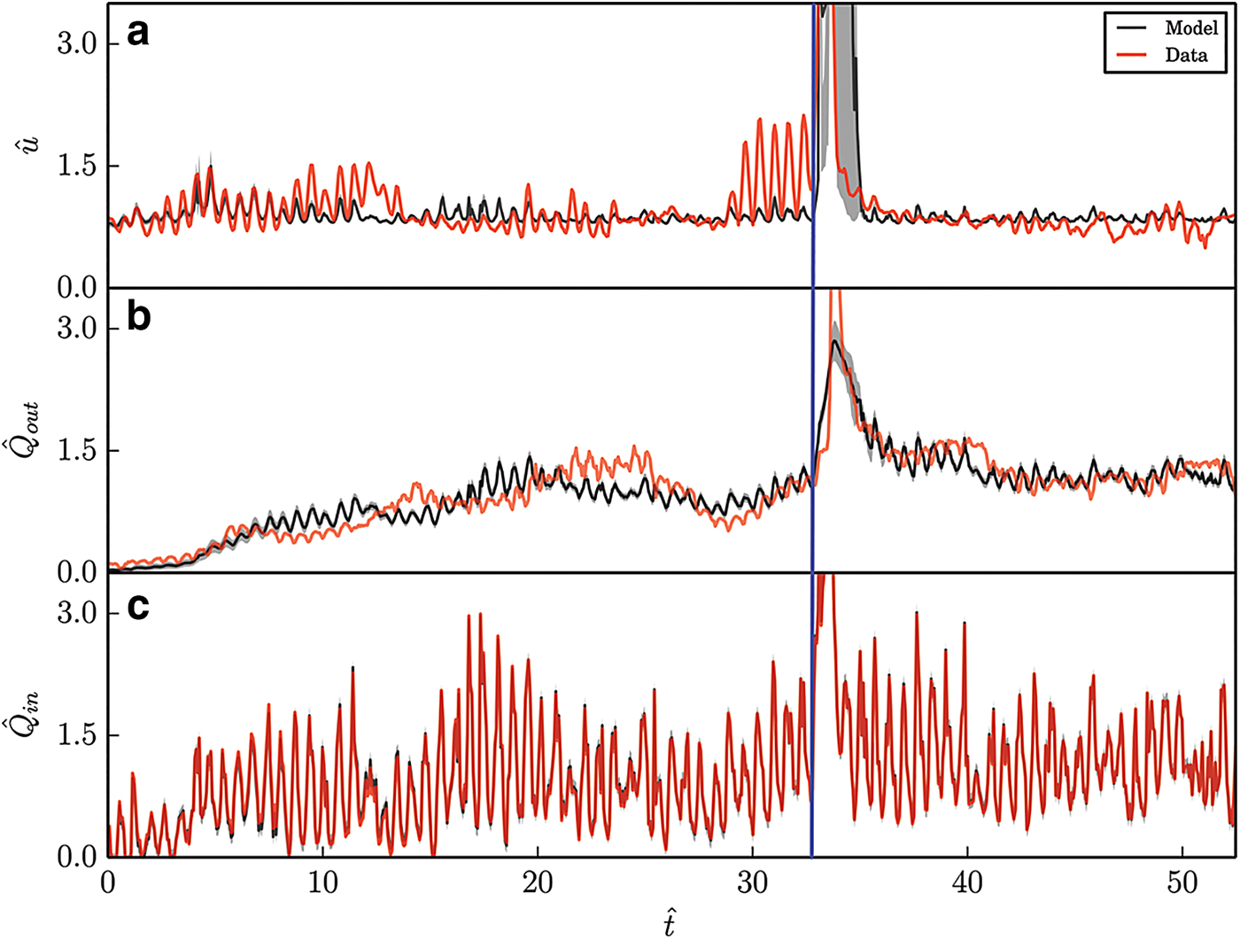
Fig. 1. Observed (red) and modelled (black) non-dimensionalized velocity, input flux and output flux. Gray envelopes correspond to the 1σ credibility interval. Blue line indicates approximate time, at which marginal lake outburst flood occurred.
MODEL DESCRIPTION
The model of the subglacial hydrologic system considered here, treats the subglacial/englacial hydrologic system as area-averaged quantities over the extent of the glacier. It is fashioned after that proposed by Bartholomaus and others (Reference Bartholomaus, Anderson and Anderson2011), with a few adaptations. Additionally, we have adopted the notation used by Bueler (Reference Bueler2014). It consists of two linked elements. First, storage of water in the englacial system is parameterized by its proxy water pressure P(t). In particular, under the assumption of an englacial drainage system that is macroporous and well connected to the subglacial system, storage in the englacial system defines a water table, which corresponds directly to subglacial water pressure. Thus, the water pressure in the englacial system is given by a simple mass budget
 $$\displaystyle{{{\rm d}P} \over {{\rm d}t}} = \displaystyle{{{\rho _{\rm w}}g} \over {LW\phi}} \left( {{Q_{{\rm in}}}(t) - {Q_{{\rm out}}}(t) - \displaystyle{{\,fLW} \over h}\displaystyle{{{\rm d}{A_{\rm c}}} \over {{\rm d}t}}} \right),$$
where L and W are the glacier length and width, respectively, ϕ the englacial porosity, h an average bedrock bump height and f a geometric factor related to the geometry of bedrock bumps. The essential statement of this equation is that the change in water pressure is governed by the flux into the system from the surface minus the flux out the terminus, less the change in capacity of the subglacial system.
Average cavity size A c(t) (a proxy for subglacial storage) is governed by the opening of cavities due to sliding, the melting of cavities due to turbulent heat generation and creep closure (Nye, Reference Nye1976)
 $$\eqalign{\displaystyle{{{\rm d}{A_{\rm c}}} \over {{\rm d}t}} &= {u_{\rm b}}h \cr &\quad + \left( {\displaystyle{{1 - {\gamma _{\rm r}}} \over {{\rho _{\rm i}}{L_{\rm f}}}}} \right)\left( {\displaystyle{{{\lambda _x}} \over W}{Q_{{\rm out}}}(t)} \right)\nabla P \cr &\quad - {C_{\rm c}}{A_{\rm c}}{({P_0} - P)^n},} $$
where u
b is the sliding velocity, γ
r the Röthlisberger constant (Röthlisberger, Reference Röthlisberger1972), C
c = 2/(Bn)
n
an effective ice softness and $\nabla P$
the hydraulic gradient, which we henceforth approximate as
$\nabla P$
the hydraulic gradient, which we henceforth approximate as $\nabla P \approx (P/\ell )$
, where ℓ is a water pressure gradient length scale. P
0 denotes the ice overburden pressure. A
c(t) is constrained to be positive, which reflects the fact that a cavity cannot possess negative cross-sectional area. P(t) is constrained to lie between zero and P
0. The lower bound reflects that, it is unlikely for a subglacial cavity to hold a vacuum (e.g. Schoof and others, Reference Schoof, Hewitt and Werder2012). Properly, the upper bound on pressure should be (ρ
w/ρ
i)P
0, where ρ
w and ρ
i are water and ice density, respectively. This bound is the limit at which the englacial water table would overtop the glacier itself, assuming a well-connected englacial cavity network, as is thought to be the case at Kennicott Glacier (Bartholomaus and others, Reference Bartholomaus, Anderson and Anderson2011). Nonetheless, our chosen sliding law becomes singular at pressures greater than overburden (which reflects the entire glacier reaching flotation), as it was developed without the consideration of either well-connectedness or more exotic mechanisms by which overburden pressure can be exceeded such as hydrofracturing (Tsai and Rice, Reference Tsai and Rice2010). As such, we impose this more restrictive constraint.
$\nabla P \approx (P/\ell )$
, where ℓ is a water pressure gradient length scale. P
0 denotes the ice overburden pressure. A
c(t) is constrained to be positive, which reflects the fact that a cavity cannot possess negative cross-sectional area. P(t) is constrained to lie between zero and P
0. The lower bound reflects that, it is unlikely for a subglacial cavity to hold a vacuum (e.g. Schoof and others, Reference Schoof, Hewitt and Werder2012). Properly, the upper bound on pressure should be (ρ
w/ρ
i)P
0, where ρ
w and ρ
i are water and ice density, respectively. This bound is the limit at which the englacial water table would overtop the glacier itself, assuming a well-connected englacial cavity network, as is thought to be the case at Kennicott Glacier (Bartholomaus and others, Reference Bartholomaus, Anderson and Anderson2011). Nonetheless, our chosen sliding law becomes singular at pressures greater than overburden (which reflects the entire glacier reaching flotation), as it was developed without the consideration of either well-connectedness or more exotic mechanisms by which overburden pressure can be exceeded such as hydrofracturing (Tsai and Rice, Reference Tsai and Rice2010). As such, we impose this more restrictive constraint.
The forcing function Q in(t) is specified by data. Bartholomaus and others (Reference Bartholomaus, Anderson and Anderson2011) also consider Q out(t) as known, but this amounts to the specification of both an influx and outflux boundary condition. This is problematic from a physical perspective and amounts to the odd conceptual situation of a fixed volume pump being attached to both ends of the hydrologic system. Such a configuration implies that the model is permanently sensitive to the initial pressure, as there is no mechanism for the self-correction of over- and under-pressure, which has serious implications for the interpretation of recovered parameter values.
Here we take an alternative approach: rather than specify the output flux, we use a generalized Manning relationship relating water pressure and channel size to output flux (e.g. Walder, Reference Walder1986), namely
 $${Q_{{\rm out}}}(t) = rA_{\rm c}^\alpha {\left( {\displaystyle{P \over \ell}} \right)^{\beta - 1}},$$
where the hydraulic gradient has again been approximated as proportional to water pressure over a gradient length scale ℓ.
To close the model, we require a constitutive relationship for basal velocity. After Bartholomaus and others (Reference Bartholomaus, Anderson and Anderson2011), we adopt the commonly used sliding law
 $${u_{\rm b}} = \displaystyle{{k\tau _{\rm b}^n} \over {{{({P_0} - P)}^\gamma}}}, $$
where k is a constant, and τ b is the basal shear stress (e.g. Bindschadler, Reference Bindschadler1983; Jansson, Reference Jansson1995). Despite notable limitations, this sliding law is simple and has been used extensively in the literature, allowing the specification of reasonable prior information about the value of its flow exponent.
Non-dimensionalization
The model described above has 23 parameters. Many of these are well constrained (e.g. physical constants like g). However, many are not. For example, the value of the geometric factor f, which describes the ratio of asperity size to spacing, is not practically observable. Simultaneously, it multiplies another under-constrained parameter ϕ, the englacial porosity. This is problematic: these two parameters could take on vastly different values, but so long as their product remained the same, the model would produce the same result. Stated another way, these parameters are not independent: the value of one depends on the other. Many such dependent pairings of parameters exist in models of subglacial hydrology. Given that their behavior cannot be independently deduced, it makes sense to treat them as a single parameter.
A formal process of non-dimensionalization indentifies independent parameters, while simultaneously scaling the value of the state variables to be ${\rm {\cal O}}(1)$
. We denote non-dimensional parameters with a hat, and their associated scaling factor with a tilde. We introduce the following relations:
${\rm {\cal O}}(1)$
. We denote non-dimensional parameters with a hat, and their associated scaling factor with a tilde. We introduce the following relations:
 $$\eqalign{& {A_{\rm c}} = {\widetilde A}\hat A,\quad P = {\widetilde P}\hat P,\quad t = {\widetilde t}\hat t, \cr & {Q_i} = {\widetilde Q}{{\hat Q}_i},\quad {u_{\rm b}} = {\widetilde u}{{\hat u}_{\rm b}},\quad k = {\widetilde k}\hat k,\quad r = {\widetilde r}\hat r.} $$
Some scaling factors emerge naturally from data. We define ${\widetilde P} = {P_0}$
, such that pressure scales from 0 at atmospheric pressure to unity at overburden. We scale the flux terms by
${\widetilde P} = {P_0}$
, such that pressure scales from 0 at atmospheric pressure to unity at overburden. We scale the flux terms by ${\widetilde Q} = {\bf E}[{Q_{{\rm obs}}}]$
, where
${\widetilde Q} = {\bf E}[{Q_{{\rm obs}}}]$
, where ${\bf E}[{Q_{{\rm obs}}}]$
is the mean of the available output flux data (and due to mass conservation, quite near the mean of the input flux data). Similarly, we scale basal velocity by choosing
${\bf E}[{Q_{{\rm obs}}}]$
is the mean of the available output flux data (and due to mass conservation, quite near the mean of the input flux data). Similarly, we scale basal velocity by choosing ${\widetilde u}$
to be the mean of the observed surface velocities. With these scales fixed, we choose the remaining ones such that the number of parameters remaining in the model is minimized. Although several parameterizations exist, we choose to use the following scaling:
${\widetilde u}$
to be the mean of the observed surface velocities. With these scales fixed, we choose the remaining ones such that the number of parameters remaining in the model is minimized. Although several parameterizations exist, we choose to use the following scaling:
 $${\widetilde t} = \displaystyle{1 \over {{C_{\rm c}}P_0^n}} $$
 $$\hskip-12pt {\widetilde A} = {\widetilde t}{\widetilde u}h$$
 $$\hskip29pt {\widetilde r} = \displaystyle{{{\widetilde Q}} \over {{{{\widetilde A}}^\alpha} {{({P_0}/l)}^{\beta - 1}}}}$$
 $$\hskip 8pt {\widetilde k} = P_0^\gamma {\widetilde u}\tau _{\rm b}^{ - n}. $$
Substituting these non-dimensional parameters and substituting the constitutive relationships for flux and velocity into the state equations produces the following non-dimensional model:
 $$\displaystyle{{{\rm d}\hat A} \over {{\rm d}\hat t}} = \displaystyle{{\hat k} \over {{{(1 - {\hat P})}^\gamma}}} + \Psi \hat r{\hat A^\alpha} {\hat P^\beta} - \hat A{(1 - {\hat P})^n}$$
 $$\displaystyle{{{\rm d}\hat P} \over {{\rm d}\hat t}} = \chi \left( {{{\hat Q}_{{\rm in}}}(\hat t) - \hat r{{\hat A}^\alpha} {{\hat P}^{\,\beta - 1}} - \Pi \displaystyle{{{\rm d}\hat A} \over {{\rm d}\hat t}}} \right),$$
where we have introduced the non-dimensional parameters
 $$\Psi = (1 - {\gamma _{\rm r}})\left( {\displaystyle{{{P_0}} \over {{\,\rho _{\rm i}}\ell {L_{\rm f}}}}} \right)\left( {\displaystyle{{{\lambda _x}} \over W}} \right)\displaystyle{{{\widetilde Q}{\widetilde t}} \over {{\widetilde A}}}$$
 $$\chi = \left( {\displaystyle{{{\rho _{\rm w}}g} \over {LW\phi}}} \right)\displaystyle{{{\widetilde Q}{\widetilde t}} \over {{P_0}}}$$
 $$\Pi = \left( {\displaystyle{{\,fLW} \over h}} \right)\displaystyle{{{\widetilde A}} \over {{\widetilde t}{\widetilde Q}}}.$$
Each of these groups acts to scale a particular term: Ψ serves to determine the relative importance of turbulent heat generation on cavity opening, χ gives the degree to which changes in englacial storage modulate fluxes, and Π governs the exchange rate between englacial and subglacial systems.
In addition to the parameters derived from non-dimensionalization, the model has two constitutive parameters $\hat k$
and
$\hat k$
and $\hat r$
that linearly scale the velocity and flux terms, respectively.
$\hat r$
that linearly scale the velocity and flux terms, respectively. $\hat k$
in particular can be thought of as a non-dimensional basal traction. Note that it would be possible to choose a scaling that eliminates
$\hat k$
in particular can be thought of as a non-dimensional basal traction. Note that it would be possible to choose a scaling that eliminates $\hat k$
, and reduces the number of parameters by one. However, in so doing we would lose the means to redimensionalize velocity, which is critical for inverse methods involving velocity data.
$\hat k$
, and reduces the number of parameters by one. However, in so doing we would lose the means to redimensionalize velocity, which is critical for inverse methods involving velocity data.
Finally, the model depends on three exponents. γ is the nonlinear dependence of sliding speed on effective pressure, while α and β relate average cavity size and pressure to discharge via the Manning relation.
INVERSION
As discussed in the section Model Description, our chosen glacier hydrology model has eight parameters describing its dynamical evolution, and we seek to estimate these parameters with the given observations, described in the section Data. We approach the matter of parameter estimation from the perspective of Bayesian inference. Bayes' theorem (e.g. Tarantola, Reference Tarantola2005) provides a means to compute the distribution of parameter values, given prior assumptions about parameter values coupled with data according to the following formula:
 $$P({\bf m} \vert {\bf d}) \propto P({\bf d} \vert {\bf m})P({\bf m}),$$
where ${\bf m}$
is the vector of model parameters,
${\bf m}$
is the vector of model parameters, ${\bf d}$
is the vector of observations and P( · ) denotes a probability density. The first term on the right-hand side is known as the likelihood. This quantifies the probability of observing the data given a particular value of
${\bf d}$
is the vector of observations and P( · ) denotes a probability density. The first term on the right-hand side is known as the likelihood. This quantifies the probability of observing the data given a particular value of ${\bf m}$
. The second term is a prior probability (or simply ‘prior’), or the presupposed distribution of parameter values prior to the consideration of the data. The left-hand side of Bayes' theorem is referred to as the posterior probability, or the probability distribution of a given parameter after having considered the data. With this probability distribution in hand, it is trivial to determine the most likely parameters, and under certain assumptions, this procedure is equivalent to minimizing a least-squares misfit function. However, possessing the complete distribution also gives us a rigorous assessment of parameter covariance.
${\bf m}$
. The second term is a prior probability (or simply ‘prior’), or the presupposed distribution of parameter values prior to the consideration of the data. The left-hand side of Bayes' theorem is referred to as the posterior probability, or the probability distribution of a given parameter after having considered the data. With this probability distribution in hand, it is trivial to determine the most likely parameters, and under certain assumptions, this procedure is equivalent to minimizing a least-squares misfit function. However, possessing the complete distribution also gives us a rigorous assessment of parameter covariance.
To specify a likelihood model, we assume that observations of both discharge and surface velocity are independent and normally distributed around the true value at each data point with pointwise variances $\sigma _{Q,i}^2 $
and
$\sigma _{Q,i}^2 $
and $\sigma _{u,j}^2 $
. Thus the likelihood is
$\sigma _{u,j}^2 $
. Thus the likelihood is
 $$\eqalign{P({\bf d} \vert {\bf m}) \propto & \prod\limits_{i \in n} {\rm exp}\left( { - \displaystyle{{{{({{\hat Q}_{{\rm out}}}({{\hat t}_i},{\bf m}) - {{\hat Q}_{{\rm obs},i}})}^2}} \over {2\sigma _{Q,i}^2}}} \right) \cr & \times \prod\limits_{\,j \in k} {\rm exp}\left( { - \displaystyle{{{{({{\hat u}_s}({{\hat t}_j},{\bf m}) - {{\hat u}_{{\rm obs},j}})}^2}} \over {2\sigma _{u,j}^2}}} \right),} $$
where n and k are the number of discharge and velocity measurements.
Selection of the data variances is somewhat subjective. While the measurements themselves are sufficiently precise to be considered nearly error-free, we note that these measurements are necessarily point measurements, and that the model produces only area-averaged quantities. As such, the specified variances should be interpreted as including the uncertainty induced by extrapolating from a point measurement to the area average over the glacier. We suppose uncertainties similar to the magnitude of the diurnal fluctuations. For the velocity estimate this is ~σ u = 0.4, and for discharge σ Q = 0.6. We also note here that we do not consider the velocity data during the flood and the enhanced diurnal signals leading up to it, as we would not expect the assumed sliding law to remain valid during such an event, where pressures are likely at or exceeding overburden (Bartholomaus and others, Reference Bartholomaus, Anderson and Anderson2011).
We also need to specify priors. For the non-dimensional groups Ψ, χ and Π, we adopt a positively constrained uniform distribution, which effectively contributes no prior information aside from positivity. We truncate the prior distribution at ten. Experimentation has shown that this choice of upper bound does not affect the computed posterior distributions. We use the same prior for the velocity and flux scaling factors $\hat k$
and
$\hat k$
and $\hat r$
.
$\hat r$
.
Conversely, the value of the constitutive exponent γ is fairly well constrained by previous studies (Jansson, Reference Jansson1995; Sugiyama and Gudmundsson, Reference Sugiyama and Gudmundsson2004). We choose to model γ as
 $$\gamma {\rm \sim} {\rm ln}{\kern 1pt} {\rm {\cal N}}(\mu = - 0.95,\;\sigma = 0.3),$$
where the log-normal distribution is given by
 $${\rm ln}{\kern 1pt} {\rm {\cal N}}(x;\;\mu, \sigma ) = \displaystyle{1 \over {x\sigma \sqrt {2\pi}}} \exp \left[ { - \displaystyle{{{{(\ln x - \mu )}^2}} \over {2{\sigma ^2}}}} \right].$$
This distribution has a mean of ${\bf E}[\gamma ] \approx 0.4$
and variance Var(γ) ≈ (2/125). α and β are similarly constrained by theory, and we model these as log-normally distributed as well:
${\bf E}[\gamma ] \approx 0.4$
and variance Var(γ) ≈ (2/125). α and β are similarly constrained by theory, and we model these as log-normally distributed as well:
 $$\alpha {\rm \sim} {\rm ln}{\kern 1pt} {\rm {\cal N}}(0.35,\;0.32)$$
 $$\beta - 1{\rm \sim} {\rm ln}{\kern 1pt} {\rm {\cal N}}( - 0.78,\;0.43),$$
which have expected values of ${\bf E}[\alpha ] \approx (3/2)$
and
${\bf E}[\alpha ] \approx (3/2)$
and ${\bf E}[\beta ] \approx (3/2)$
, respectively, corresponding to common literature values (e.g Fowler, Reference Fowler1986; Werder and others, Reference Werder, Hewitt, Schoof and Flowers2013). The variance for each of these distributions is Var(α) ≈ (1/4) and Var(β) ≈ (1/20). We note that, while the mean of each of these distributions was chosen to correspond to published values, the variances were specified heuristically; in the absence of any rigorous empirical estimates of variance, we chose values that seemed to provide a plausible estimate of values that these parameters might assume.
${\bf E}[\beta ] \approx (3/2)$
, respectively, corresponding to common literature values (e.g Fowler, Reference Fowler1986; Werder and others, Reference Werder, Hewitt, Schoof and Flowers2013). The variance for each of these distributions is Var(α) ≈ (1/4) and Var(β) ≈ (1/20). We note that, while the mean of each of these distributions was chosen to correspond to published values, the variances were specified heuristically; in the absence of any rigorous empirical estimates of variance, we chose values that seemed to provide a plausible estimate of values that these parameters might assume.
In addition to the eight governing parameters, we must also include uncertainty in the input function ${\hat Q_{{\rm in}}}$
and in converting from basal velocity
${\hat Q_{{\rm in}}}$
and in converting from basal velocity ${\hat u_{\rm b}}$
, which is modelled, to surface velocity
${\hat u_{\rm b}}$
, which is modelled, to surface velocity ${\hat u_{\rm s}}$
, which is observed by estimating the deformational velocity
${\hat u_{\rm s}}$
, which is observed by estimating the deformational velocity ${\hat u_{\rm d}}$
. Effectively, this means that we must assign prior distributions to each of these quantities and include them as additional parameters in the inversion.
${\hat u_{\rm d}}$
. Effectively, this means that we must assign prior distributions to each of these quantities and include them as additional parameters in the inversion.
We model uncertainty in ${\hat Q_{{\rm in}}}(\hat t)$
as a multivariate normal distribution with a mean given by value from a positive degree-day model and a Gaussian covariance with correlation timescale τ = 1 (i.e. random variations occur smoothly and over the characteristic timescale of the differential equation), which in dimensional time corresponds to τ ≈ 1.4 d. We assume a standard deviation of σ
in = 0.2.
${\hat Q_{{\rm in}}}(\hat t)$
as a multivariate normal distribution with a mean given by value from a positive degree-day model and a Gaussian covariance with correlation timescale τ = 1 (i.e. random variations occur smoothly and over the characteristic timescale of the differential equation), which in dimensional time corresponds to τ ≈ 1.4 d. We assume a standard deviation of σ
in = 0.2.
Basal velocities produced by the forward model are not directly comparable with the surface velocity data, and we do not know a priori the proportion of the surface velocity accounted for by deformational velocity ${\hat u_{\rm d}}$
. To account for this, we assume that
${\hat u_{\rm d}}$
. To account for this, we assume that
 $${\hat u_{\rm s}}(\hat t) = {\hat u_{\rm b}}(\hat t) + {\hat u_{\rm d}},$$
where ${\hat u_{\rm d}}$
is given by
${\hat u_{\rm d}}$
is given by
 $${\hat u_{\rm d}}{\rm \sim} {\rm Unif}(0,\;{\rm min}({\hat u_{{\rm obs}}})).$$
This implies that the surface velocity is the sum of a modelled time-varying basal velocity, and a constant but unknown deformational velocity. The deformational velocity may, as end-member cases, account for either none of the surface velocity or all of the velocity signal minus the time-varying component. This is a more conservative assumption than modelling deformational velocities; the shallow-ice approximation would not yield an accurate result in this context, and we have insufficient geometric information to model higher-order stresses.
Finally, we also specify log-normally distributed priors for the initial conditions on $\hat P$
and
$\hat P$
and ${\hat A}_{\rm c}$$
 $$\hat P(\hat t = 0){\rm \sim }{\rm ln}{\kern 1pt} {\rm {\cal N}}( - 1.12,\;0.64)$$
 $${\hat A}_{\rm c}(\hat t = 0){\rm \sim} {\rm ln}{\kern 1pt} {\rm {\cal N}}(0.49,\;0.64),$$
which enforce non-negativity but otherwise provide relatively little information. Experimentation has shown that the choice of initial conditions has a minimal effect on model results, and that after a short ( $ \approx \hat t = 1$
) equilibration period, even extremely improbable initial conditions yield very similar solutions to more reasonable ones.
$ \approx \hat t = 1$
) equilibration period, even extremely improbable initial conditions yield very similar solutions to more reasonable ones.
Sampling
The posterior distribution cannot be computed directly, and must be characterized with samples instead. With a large number of these in hand, we can then evaluate the statistical properties of the samples as a proxy for the joint posterior distribution of the parameters.
There are many choices of sampling algorithm, but we chose the Adaptive Metropolis Algorithm (AMA) (Haario and others, Reference Haario, Saksman and Tamminen2001), which is a variant of the classic Metropolis–Hastings (MH) algorithm (Hastings, Reference Hastings1970). The MH algorithm works by travelling through parameter space, sequentially updating each parameter independently by randomly drawing a jump from a proposal distribution. If the posterior probability is greater at the new location than at the present, the new parameter value is accepted. Otherwise, it is accepted with probability proportional to the ratio of the current posterior probability and that of the proposed value.
The AMA functions identically, except that the proposal distribution is updated by iteratively constructing a covariance matrix from the previous samples, and proposing a new parameter set en masse, rather than individually. This variant is particularly suited for this problem, where parameters tend to be strongly correlated and the covariance matrix can help to identify suitable proposal steps. Simultaneously, by block updating the parameters, the number of forward model evaluations is reduced, increasing efficiency. We use the implementation of these algorithms available in the PyMC package (Patil and others, Reference Patil, Huard and Fonnesbeck2010).
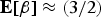
We drew 5 × 10⁵ samples from the joint posterior distribution of the parameters given in Table 2, repeated three times in order to assess consistency between sample populations. In order to assess convergence, we relied upon a heuristic examination of the history of each parameter as it was sampled; well-converged sample populations typically traverse the feasible parameter space many times (Fig. 2a). Additionally, we compared sample histograms between populations to assess whether the posterior distribution was unique (Fig. 2b). As a numerical convergence test, we computed the Gelman–Rubin statistic (Gelman and Rubin, Reference Gelman, Rubin, Bernardo, Berger, Dawid and Smith1992), which compares the intra-population variance with the inter-population variance. In the limit as the sample size goes to infinity, the Gelman–Rubin statistic R converges to unity. A well-converged sample set that exhibits limiting statistical behavior should also have an R value near one. In our case, for each parameter tested R ≪ 1.1, which is typically taken to indicate adequate convergence.
Fig. 2. (a) Sampling history of each state parameter. The fuzzy appearance is an indicator of the algorithm efficiently and fully exploring the feasible parameter space. (b) Histograms of each parameter's marginal distribution for three independently sampled parameter populations. The identical posterior distributions strongly indicate population convergence.
Table 1. Dimensional constants and their values as used by Bartholomaus and others (Reference Bartholomaus, Anderson and Anderson2011)

Table 2. Parameters computed using the constants defined in Table 1 (column 2) and the maximum a posteriori probability (MAP) parameter estimates determined using the methods described in this paper (column 3)

RESULTS AND DISCUSSION
State variables
Figure 1a shows the posterior distribution of velocity along with velocity observations. It is immediately evident that the model reproduces the long-timescale variability in velocity observations well. Additionally, we see that the model is also capable of reproducing diurnal variability in both magnitude and duration. The good fidelity to diurnal timing should not be surprising: these features are forced by the input data, and the input data exhibit the same structure, as seen in Figure 1c. Adequately reproducing the magnitude of velocity fluctuations is more difficult and more important, as this imposes strong constraints on pressure.
One case where the model does not reproduce the velocity observations well is during and before the flood that occurred at $\hat t \approx 32$
. Although it is not well shown in Figure 1a, the model predicts velocities of approximately twice those observed, with a broader peak. Two observations seem relevant here. First, this misfit is likely due to inadequacies in the sliding law both in the sense that it is not well equipped to handle pressures very near overburden, and also because it is unable to include effects that would serve to mitigate the velocity increase, such as longitudinal and transverse stresses. Secondly, the large diurnal fluctuations evident before the main velocity peak indicate that processes occur that are either not captured by the input data or are not captured by the model physics. An example of the former would be an additional pre-emptive lake drainage or other anomalous source of extra water. This seems unlikely, as such an input would appear in the output flux data, which it does not. An example of the latter could be the inability of the model to capture local hydraulic jacking effects due to the lake partially draining and subsequently refilling, without overcoming the necessary pressure barrier to route excess water into the greater subglacial drainage system.
$\hat t \approx 32$
. Although it is not well shown in Figure 1a, the model predicts velocities of approximately twice those observed, with a broader peak. Two observations seem relevant here. First, this misfit is likely due to inadequacies in the sliding law both in the sense that it is not well equipped to handle pressures very near overburden, and also because it is unable to include effects that would serve to mitigate the velocity increase, such as longitudinal and transverse stresses. Secondly, the large diurnal fluctuations evident before the main velocity peak indicate that processes occur that are either not captured by the input data or are not captured by the model physics. An example of the former would be an additional pre-emptive lake drainage or other anomalous source of extra water. This seems unlikely, as such an input would appear in the output flux data, which it does not. An example of the latter could be the inability of the model to capture local hydraulic jacking effects due to the lake partially draining and subsequently refilling, without overcoming the necessary pressure barrier to route excess water into the greater subglacial drainage system.
Figure 1b shows the posterior distribution of modelled output flux along with observations. Once again, the model effectively captures both the long-term variability in output flux, as well as the frequency and magnitude of diurnal variability. However, as with the modelled velocity, some limitations are evident. First, the modelled output fluxes are offset by around half a diurnal period. This is the result of the spatially averaged nature of the model, particularly the fact that pressure is assumed to propagate instantaneously through the system, and output flux responds immediately to variations in input flux. In reality, pressure changes induced in the upper reaches of the system would take some amount of time to propagate downgradient, and this propagation time would be dependent upon the state of the hydrologic system.
Another notable instance where the model fails to reproduce observations occurs just prior to the flood event. Here input and output fluxes are out of phase with one another by around ten diurnal cycles. This too could be a result of the lack of spatially heterogeneous storage. This misfit is less pronounced or non-existent following the flood. An explanation for this is that the drainage system has grown more efficient, causing the implicit assumption of uniform spatial response times to become a better approximation to reality. This modelled increase in cavity size is evident in Figure 3c, which shows a marked increase in average cavity size following the flood. As cavities become larger (and presumably better connected), we would expect the lumped model to capture the temporal variability of the system with more fidelity.
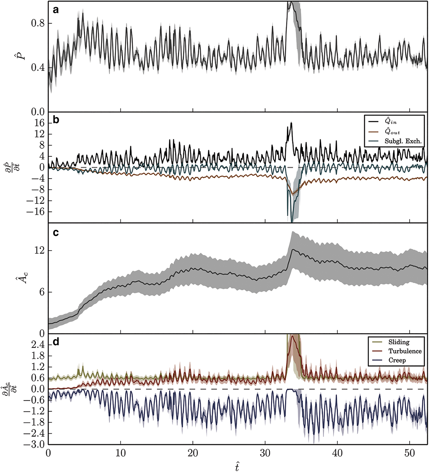
Fig. 3. Posterior distributions and observations of non-dimensional pressure (a), magnitude of pressure model terms (b), average cavity size (c), magnitude of cavity model terms (d).
The modelled englacial water pressure as a fraction of overburden is shown in Figure 3a. While no direct observations of water pressure are available, we observe that the model reproduces the expected diurnal fluctuations, and that under non-flood conditions, the glacier tends to oscillate between ~40% and 80% of overburden. The magnitude of the modelled fluctuations is similar to observations in many mountain glaciers (Amundson and others, Reference Amundson, Truffer and Lüthi2006; Harper and others, Reference Harper, Humphrey, Pfeffer and Lazar2007), lending support to the reliability of predictions. During the flood event, the pressure increases to overburden (which it is constrained not to exceed), though the uncertainty during this event is high.
We can also examine the relative magnitude of each mechanism contributing to the evolution of the water pressure on a termwise basis. Figure 3b shows the individual contributions of the input flux, output flux and subglacial exchange terms through time. For dynamic equilibrium to occur (i.e. no long-term storage change), the three terms, on average, must sum to zero, which they do less the water moving out of subglacial storage and into englacial storage. Input flux and output flux are both uniformly and respectively positive and negative (by definition). The more interesting contributor to the evolution of the pressure state is the subglacial/englacial exchange term Π, which acts as a buffer for the large swings in input flux, while maintaining an approximately zero mean. This short-term fluctuation in subglacial storage is responsible for the evident attenuation in flux magnitude between input and output. Note that in Figure 3b, a positive value of the subglacial exchange term implies that water is moving into englacial storage from subglacial storage. Predictably, this state occurs when water pressure is low, and creep closure acts to drive water out of cavities.
Figure 3b shows the non-dimensional cavity size. While we cannot compute the dimensional constant ${\widetilde A}$
that would be necessary to re-dimensionalize the modelled cavity size, we note that the (known) time and velocity scales imply that, it is of the same order as the bedrock bump height. As such,
${\widetilde A}$
that would be necessary to re-dimensionalize the modelled cavity size, we note that the (known) time and velocity scales imply that, it is of the same order as the bedrock bump height. As such, $\hat A$
is similar to A
c so long as average bedrock asperities are on the order of meters in height. We first note that the variance in cavity size distribution is higher than the other state variables. This implies that the parameters controlling it cannot be precisely determined given the available data. Alternatively, it would appear that the specifics of cavity formation play a less critical role in explaining surface velocity and output flux than does the pressure, commensurately limiting the amount of information that can be used to constrain its governing parameters. Nonetheless, it remains possible to make a qualitative assessment of cavity evolution over the modelled time period. At the beginning of the simulation, cavities are relatively small. The cavities grow during pressure-driven speed-up events, but the increasingly well-developed cavities tend to damp this response as time goes on. During the lake drainage event, the average cavity size increases significantly. This increase in size decays over the course of a few days, as the reduced water pressure following drainage is no longer capable of sustaining large cavities and creep closure becomes the dominant mechanism of channel evolution.
$\hat A$
is similar to A
c so long as average bedrock asperities are on the order of meters in height. We first note that the variance in cavity size distribution is higher than the other state variables. This implies that the parameters controlling it cannot be precisely determined given the available data. Alternatively, it would appear that the specifics of cavity formation play a less critical role in explaining surface velocity and output flux than does the pressure, commensurately limiting the amount of information that can be used to constrain its governing parameters. Nonetheless, it remains possible to make a qualitative assessment of cavity evolution over the modelled time period. At the beginning of the simulation, cavities are relatively small. The cavities grow during pressure-driven speed-up events, but the increasingly well-developed cavities tend to damp this response as time goes on. During the lake drainage event, the average cavity size increases significantly. This increase in size decays over the course of a few days, as the reduced water pressure following drainage is no longer capable of sustaining large cavities and creep closure becomes the dominant mechanism of channel evolution.
Once again, it is useful to examine each modelled mechanism's contribution to cavity evolution (Fig. 3d). Near the beginning of the simulation when cavities are small, sliding is the dominant mechanism of cavity opening. During this stage, there is insufficient flux through the cavities to support the production of much turbulent heat. Simultaneously, creep closure has yet to act strongly, because the cavities are still relatively small and the closure rate scales linearly with cavity area. As the cavities grow, opening due to bedrock sliding remains relatively constant, while both turbulent dissipation and creep closure grow in magnitude. Creep closure in particular exhibits strong diurnal variations as the large variations in water pressure are amplified by the nonlinearity in ice rheology, with nearly no closure occurring when effective pressures are near zero. In particular, during the highly pressurized flood event, creep closure effectively shuts down for several days, while both enhanced basal sliding and increased output flux rapidly enlarge subglacial cavities.
Evaluating the uncertainties associated with each term in Eqn (7) gives us an understanding of the source of the relatively large degree of uncertainty associated with cavity size. In particular, we see that the cavity opening rate is subject to a much larger relative degree of uncertainty than other terms in Figure 3d, and it is this uncertainty that generates the large spread evident in Figure 3c. The greater degree of uncertainty in the magnitude of this term is to be expected; like opening due to sliding, dissipative heating is directly associated with one of the observed quantities (namely output flux). However, unlike opening due to sliding, dissipative heating is associated with the additional free parameter Ψ apart from the constitutive flux relation.
Finally, we can look at the posterior distribution of the deformation velocity and initial conditions (Fig. 4). In the case of deformational velocities, the model has a slight tendency towards predicting deformational velocities near the center of the admissible range. Due to the insensitivity of model dynamics to initial conditions, the posterior distributions of both initial conditions are very similar to their prior distributions. In general, the inversion procedure contributes little useful information towards these parameters, and in this context they should be viewed primarily as sources of additional uncertainty with respect to the other model parameters.
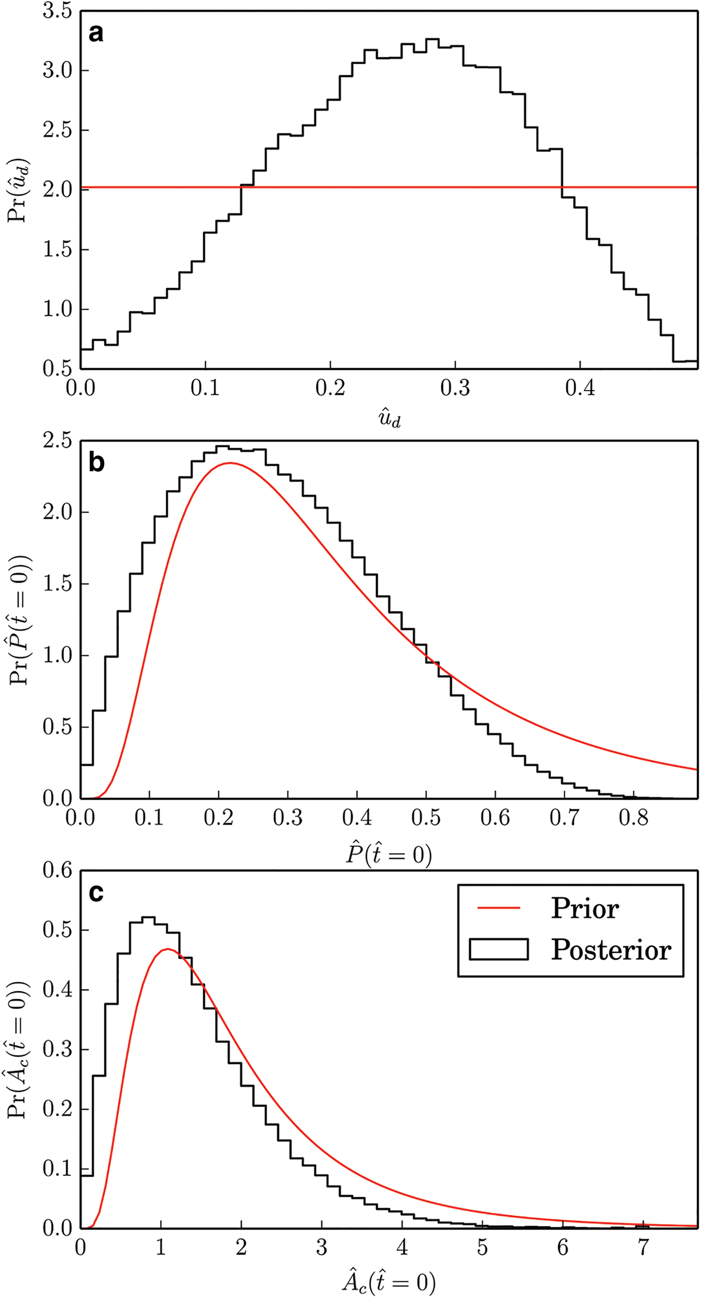
Fig. 4. Posterior distributions of peripheral variables deformational velocity u
d, pressure initial condition $\hat P(\hat t = 0)$
and cavity area initial condition
$\hat P(\hat t = 0)$
and cavity area initial condition ${\hat A}_{\rm c}(\hat t = 0)$
.
${\hat A}_{\rm c}(\hat t = 0)$
.
CONFIGURATION STABILITY
Because we have in our model included turbulent heat generation as a mechanism for melting cavity walls, we must also assess whether or not our envisaged drainage configuration is compatible with the parameter values that we have recovered from a stability perspective. A well-known result from Kamb (Reference Kamb1987) shows that for water pressures above a threshold value and a given hydraulic gradient, a linked cavity system undergoes runaway evolution towards a channelized system. We note these results, and the similar ones found in, for example, Schoof (Reference Schoof2010) and Hewitt (Reference Hewitt2011) are based on linear stability analysis, and only strictly valid for autonomous systems of equations. The inclusion of a time-varying influx term clearly makes this system of equations non-autonomous, and the analysis of the stability of such systems is beyond the scope of this paper. Nonetheless, we can find model steady states for a prescribed steady influx (i.e. a fixed ${\hat Q_{{\rm in}}}$
as opposed to a time-varying one) in order to assess the stable states of the model.
${\hat Q_{{\rm in}}}$
as opposed to a time-varying one) in order to assess the stable states of the model.
In steady state, Eqns (7) and (8) reduce to
 $${\hat A}_{\rm c} = (1 - {\hat P})^n\left[ {\displaystyle{{\hat k} \over {{{(1 - {\hat P})}^\gamma}}} + \Psi {{\hat Q}_{{\rm in}}}{\hat P}} \right]$$
 $$0 = {{\hat Q}_{{\rm in}}} - {\hat r}{\hat A}_{\rm c}^{\alpha} {{\hat P}^{\beta - 1}},$$
the numerical solution of which is straightforward to compute. Furthermore, we can compute the stability of each of these points by evaluating the eigenvalues of the Jacobian matrix of Eqns (7) and (8). Doing so for the parameters computed through inversion yields the interesting result that regardless of the chosen flux, the system has a unique and stable steady state. This is held in contrast to the results of Kamb (Reference Kamb1987), Schoof (Reference Schoof2010) and Hewitt (Reference Hewitt2011), which would predict runaway channelization due to the magnitude of the turbulent melting terms included here. The reason that this model differs is that flux is fundamentally limited by the requirement of global mass conservation; runaway channel growth is not possible because such growth efficiently evacuates the water necessary to maintain the low effective pressures that limit creep closure. This occurs because the lumped structure of the model requires that this channelization occur everywhere simultaneously. In a spatially explicit model (and presumably in reality), spatial heterogeneity allows distinct channels to remain self-sustainingly pressurized by drawing upon local rather than global reservoirs. The suppression of the channelizing instability by the model structure begs the question of whether the dynamics induced by such effects can credibly be neglected. This remains an unresolved issue, and we do not claim to have the answer here. Our approach is qualitatively supported by observations at the terminus of Kennicott Glacier, where there exist no obvious subglacial channels. The Kennicott terminus is characterized by a linked series of terminal lakes, none of which has visible subglacial input. Nonetheless, we imagine that during the lake outburst flood, development of large and efficient channels becomes dominant over a distributed system due to the high water pressures involved, and the suppression of creep closure as seen in Figure 3b. During this period the model tends to overestimate the length of the perturbation in velocity (and so probably water pressure as well) due to the flood. During the lake drainage, we speculate that a channel developed, which evacuated water much more quickly than this model can account for without explicit channelization.
Parameter covariance
In addition to assessing the feasible model states, possessing the joint posterior distribution allows us to examine the covariance structure of the model parameters as well. Figure 5 shows the joint sample distribution of each parameter pair, as well as the histogram of each.

Fig. 5. Histograms on the diagonal show the marginal posterior distribution of each parameter. The red line indicates the maximum posterior probability. Scatter plots below the diagonal indicate the relationship between each parameter set. Colored boxes above the diagonal indicate the correlation coefficient for each pair of parameters: red indicates a negative correlation, while blue indicates a positive one.
The first set of strongly correlated parameters are the two, which govern the sliding speed $\hat k$
and γ. This result is not surprising: given data uncertainty and the flexibility granted by their priors, there are a variety of combinations that these two parameters can feasibly adopt due to the inversely correlated relationship built into the sliding law. Nonetheless, it is worth noting that both parameters have smaller variance than their priors, indicating that the data provide information about both (recall, e.g. that the prior on
$\hat k$
and γ. This result is not surprising: given data uncertainty and the flexibility granted by their priors, there are a variety of combinations that these two parameters can feasibly adopt due to the inversely correlated relationship built into the sliding law. Nonetheless, it is worth noting that both parameters have smaller variance than their priors, indicating that the data provide information about both (recall, e.g. that the prior on $\hat k$
is uniform).
$\hat k$
is uniform). $\hat r$
and α, which control the magnitude and cavity size dependence of the flux, are correlated in a similar fashion.
$\hat r$
and α, which control the magnitude and cavity size dependence of the flux, are correlated in a similar fashion.
A more interesting negative correlation exists between Π, the parameter scaling the importance of englacial/subglacial exchange, and Ψ, the parameter controlling the rate of turbulent melting. In particular, this correlation implies that decreases in the geometric capacity for the subglacial system to store water can be offset by increases in the rate at which turbulent melting can occur. Since the magnitude of cavity opening due to bedrock sliding and closing due to creep are both constrained by the scaling of the problem, only Π and Ψ can covary. These parameters are positively and negatively correlated with α, respectively. An increase in either has the tendency to produce a greater amount of subglacial storage, but this correlation tells us that an increase in the flux dependence on ${\hat A}_{\rm c}$
is more easily offset by an increase in turbulent melt rates, than by an increase in the subglacial/englacial transfer rate as a whole.
${\hat A}_{\rm c}$
is more easily offset by an increase in turbulent melt rates, than by an increase in the subglacial/englacial transfer rate as a whole.
A final observation is that the value of χ is ${\rm {\cal O}}(1)$
. This parameter relates the size of the flux terms on the right-hand side of Eqn (8) to the rate of change of the pressure, and is effectively a proxy for englacial porosity. Previous work has suggested that this term is limitingly large, which is to say that englacial porosity is close to zero. This effectively assumes that changes in englacial storage occur instantaneously (Schoof and others, Reference Schoof, Hewitt and Werder2012), and that the time derivative appearing in Eqn (8) is zero. Other models have retained this term under the auspices of a non-negligible englacial porosity as a means to regularize a distributed model of subglacial cavity evolution (Werder and others, Reference Werder, Hewitt, Schoof and Flowers2013; Bueler and Van Pelt, Reference Bueler and Van Pelt2015). Clarke (Reference Clarke2003), though citing an alternative physical mechanism of compressibility, also included an analogous term to improve numerical stability. Our results suggest that despite the initial numerical motivation, retaining the time derivative in Eqn (8) may also be physically correct, and also that the inclusion of significant englacial storage is required to simultaneously explain observed velocity and output fluxes. This additional storage could take the form of englacial void space (Fountain and others, Reference Fountain, Jacobel, Schlichting and Jansson2005), basal crevasses (Harper and others, Reference Harper, Bradford, Humphrey and Meierbachtol2010) or a combination thereof. This further begs the question, what is the englacial macroporosity corresponding to a χ of
${\rm {\cal O}}(1)$
. This parameter relates the size of the flux terms on the right-hand side of Eqn (8) to the rate of change of the pressure, and is effectively a proxy for englacial porosity. Previous work has suggested that this term is limitingly large, which is to say that englacial porosity is close to zero. This effectively assumes that changes in englacial storage occur instantaneously (Schoof and others, Reference Schoof, Hewitt and Werder2012), and that the time derivative appearing in Eqn (8) is zero. Other models have retained this term under the auspices of a non-negligible englacial porosity as a means to regularize a distributed model of subglacial cavity evolution (Werder and others, Reference Werder, Hewitt, Schoof and Flowers2013; Bueler and Van Pelt, Reference Bueler and Van Pelt2015). Clarke (Reference Clarke2003), though citing an alternative physical mechanism of compressibility, also included an analogous term to improve numerical stability. Our results suggest that despite the initial numerical motivation, retaining the time derivative in Eqn (8) may also be physically correct, and also that the inclusion of significant englacial storage is required to simultaneously explain observed velocity and output fluxes. This additional storage could take the form of englacial void space (Fountain and others, Reference Fountain, Jacobel, Schlichting and Jansson2005), basal crevasses (Harper and others, Reference Harper, Bradford, Humphrey and Meierbachtol2010) or a combination thereof. This further begs the question, what is the englacial macroporosity corresponding to a χ of ${\rm {\cal O}}(1)$
? Assuming the length and width scales of Bartholomaus and others (Reference Bartholomaus, Anderson and Anderson2011) (see Table 2), we find that porosity must be in the range ϕ = [10−4, 10−3]. The scaling analysis in the section Non-dimensionalization shows us that even this modest amount of porosity provides a sufficient amount of storage to provide an englacial reservoir of equivalent magnitude to the subglacial reservoir.
${\rm {\cal O}}(1)$
? Assuming the length and width scales of Bartholomaus and others (Reference Bartholomaus, Anderson and Anderson2011) (see Table 2), we find that porosity must be in the range ϕ = [10−4, 10−3]. The scaling analysis in the section Non-dimensionalization shows us that even this modest amount of porosity provides a sufficient amount of storage to provide an englacial reservoir of equivalent magnitude to the subglacial reservoir.
CONCLUSIONS
We have extended the subglacial hydrology model of Bartholomaus and others (Reference Bartholomaus, Anderson and Anderson2011) in a few ways, which is ‘lumped’ in the sense that it treats the whole of the subglacial system using area-averaged quantities. An advantage of this treatment is that it allows a simple numerical treatment, as the model consists of a pair of non-homogeneous, nonlinear ordinary differential equations. Furthermore, the simplicity of the model allows for the straightforward identification of the governing parameters.
First, we have discarded the simultaneous specification of both input and output fluxes in favor of a Manning flow relation, which relates output flux to both average cavity size and water pressure. Second, we have formally non-dimensionalized the model to determine the specific parameter ratios that govern model dynamics. In so doing, we identified eight parameters. Three are non-dimensional groups controlling the relative importance of turbulent melting of cavity walls (Ψ), the exchange rate between the englacial and subglacial hydrologic systems (Π) and the rate at which the englacial water system can accommodate flux imbalances (χ). The remaining five parameters describe constitutive relationships describing both the relationship between effective pressure and basal ice velocity and the relationship between average cavity size, water pressure and outflux.
The values of these parameters are known a priori with varying degrees of certainty. We sought to improve these estimates through inverse modelling. Using flux and velocity observations from Bartholomaus and others (Reference Bartholomaus, Anderson and Anderson2011) to construct a likelihood function, and in conjunction with prior parameter estimates, we used a Markov-chain Monte Carlo method to sample from the joint posterior probability distribution of the model parameters, conditioned upon velocity and flux data from Kennicott Glacier. Not only did this allow us to determine the most probable parameter values, but also to characterize the covariance within and between parameters.
Despite the simplicity of the lumped modelling approach, we were able to reproduce observations with a reasonable degree of fidelity. The model captures both the magnitude and timing of diurnal variability in velocity and output flux, even passably capturing the dynamics of a lake-related flooding event. The model predicted diurnal water pressure variations between 40% and 80% of overburden, which corresponds well to prior observations of borehole pressure records in similar systems. The model also produced reasonable estimates of average cavity size. Nonetheless, the limitations due to the assumption of spatial uniformity were also evident, as longer scale temporal variability, particularly in the less efficient pre-flood configuration, was not captured. It is possible that adding spatial dimensionality to the model could help to reduce some of the remaining misfit, and the way forward in doing this is clear (Bueler, Reference Bueler2014). However, this would drastically increase the computatational cost of the forward model, making the rigorous estimation of parameter covariance through Monte Carlo methods less practical. Nonetheless, it would be extremely valuable to determine whether the conclusions suggested by this work hold in the presence of more advanced physics, and if not, the reason for the inconsistency.
The parameter estimates produced by the inverse modelling procedure suggested that all of the mechanisms included in the model were important in explaining observations. Cavity opening due to basal sliding seems to dominate the evolution of the subglacial system until cavities grow large enough to support turbulent heat generation, at which point the interplay between turbulent melting and creep closure become important as well. Our results also suggest that transfer of water into the subglacial hydrologic system from the englacial system acts to attenuate the input flux signal, leading to the observed relative reductions in magnitude in the diurnal variability of output flux.
Finally, we find that the assumption of negligible englacial porosity is not compatible with observations under the assumptions of the model used here, so we suppose that englacial storage plays an important role in the hydrologic systems of glaciers similar to the one examined here, even for relatively low absolute values of glacier macroporosity. Addressing this supposition further will require direct measurements of englacial porosity and connectivity in more glaciers, as well as further numerical investigation through inverse modelling. If englacial porosity indeed has a ubiquitous influence on glacier dynamics, then further effort towards quantifying and predicting this value will be required in order to credibly model the effect of hydrology on glacier dynamics.
ACKNOWLEDGEMENTS
This paper was initially conceived and developed at the International Glaciology Summer School, held in McCarthy, AK. We acknowledge the summer school's organizer Regine Hock and the support of the US National Science Foundation ARC-1204202, GlacioEx (Glaciology Exchange program funded by Norwegian Centre for International Cooperation in Higher Education, Partnership Program for North America), the International Association of Cryospheric Sciences, and the International Glaciological Society. Many thanks to Patricia Eugster for insightful conversations. We acknowledge the helpful comments of the scientific editor, Christian Schoof, and two anonymous reviewers, which greatly improved the quality of this manuscript. D. J. B. was supported by the US National Science Foundation (NSF) Graduate Research Fellowhip grant No. DGE1242789. C.R.M. was supported by the NSF Graduate Research Fellowship grant No. DGE1144152. E. B. was supported by NASA grant NNX13AM16G.


 Open access