


1. Introduction
1.1. Thermal siphon, a case of overturning circulation
Horizontal convection, or overturning circulation, can occur when surface waters are differentially heated – or cooled – across the fluid's domain. A canonical example is the ‘meridional overturning circulation’ resulting from the differential heating between equatorial and polar regions (Hughes & Griffiths Reference Hughes and Griffiths2008). Overturning circulations, however, may also arise at much smaller scales when a spatially uniform heat flux warms or cools the water surface (i.e. the air–water interface) of sloping waterbodies. In this scenario, shallows warm or cool more rapidly than deeper waters. The latter topographically controlled differential heating or cooling sets a horizontal density gradient that can drive a large-scale overturning circulation (LS-OC), also known as ‘thermal siphon’ (Monismith, Imberger & Morison Reference Monismith, Imberger and Morison1990). Such a phenomenon can be observed in nearshore zones of lakes and open seas (Fer, Lemmin & Thorpe Reference Fer, Lemmin and Thorpe2002; Ivanov et al. Reference Ivanov, Shapiro, Huthnance, Aleynik and Golovin2004; Monismith et al. Reference Monismith, Genin, Reidenbach, Yahel and Koseff2006; Bouffard & Wüest Reference Bouffard and Wüest2019), and its induced cross-shore circulation is more distinctive when wind and background currents are weak or absent (Molina et al. Reference Molina, Pawlak, Wells, Monismith and Merrifield2014; Ulloa et al. Reference Ulloa, Davis, Monismith and Pawlak2018; Ramón et al. Reference Ramón, Ulloa, Doda and Bouffard2021). The linear model introduced by Farrow & Patterson (Reference Farrow and Patterson1993) captures the underlying mechanisms responsible for the diurnal, thermally driven horizontal circulation and has been the foundation to derive analytical solutions that characterise the cross-shore flow induced by more complex forcing conditions.
In this work we investigate and characterise the transient dynamics associated with the development of thermal siphons due to surface cooling only. A summary of the major contributions focusing on the fluid dynamics of this type of convective flows is presented next.
1.2. Cooling-driven thermal siphon
Considering a wedge-like water basin of a uniform slope, the pioneering experimental and numerical work by Horsch & Stefan (Reference Horsch and Stefan1988) showed that a thermal siphon results from a cumulative process. As the thermals induced by surface cooling interact with the sloping bottom, they feed a downslope gravity current formed in the shallowest region. Due to mass conservation, the thermally driven downslope gravity current boosts a surface current towards the shore, leading to an overturning circulation. Thus, the thermal siphon is formed by a two-layer exchange flow. Its bottom layer transports colder and denser waters downslope (offshore), whereas its surface layer transports warmer and lighter waters towards the shore. Sturman, Oldham & Ivey (Reference Sturman, Oldham and Ivey1999) performed laboratory experiments to examine the horizontal exchange driven by a destabilising buoyancy flux,  $B_{0}$, imposed locally at the surface of waters that were bottom bounded by a constant slope bathymetry, $\bar {s}$, joined to a uniform-depth basin. In a steady-state regime Sturman et al. (Reference Sturman, Oldham and Ivey1999) derived a scaling for the discharge transported by the downslope gravity current and the time scale taken to flush the sloping region. Both quantities depend on $B_{0}$, $\bar {s}$ and the horizontal extent of the sloping bottom, $\ell _{s}$.
Wells & Sherman (Reference Wells and Sherman2001) studied via laboratory experiments thermal siphons using a basin composed of a flat shelf joined to a deeper flat basin through a sloping bottom, similar to the basin sketched in figure 1. Before the formation of a thermal siphon, Wells & Sherman (Reference Wells and Sherman2001) described that there was a period of active vertical mixing along which a large horizontal temperature difference was set between the shallow and deep areas. The authors estimated the initialisation of the gravity currents using the ‘transition time scale’ derived by Finnigan & Ivey (Reference Finnigan and Ivey1999) in the context of a buoyancy-driven exchange flow between two basins separated by a sill. In the problem investigated by Finnigan & Ivey (Reference Finnigan and Ivey1999), the lateral buoyancy gradient was forced by imposing a localised and destabilising surface buoyancy flux on one of the basins. Finnigan & Ivey (Reference Finnigan and Ivey1999) found that the exchange flow across the sill experienced three dynamic regimes. Initially, convection was localised in the basin subjected to the surface buoyancy flux, which led to the progressive growth of the density difference between both basins. At one point, the system developed a transient exchange flow across the sill until achieving a quasi-steady state. The characterisation of the regime associated with horizontal convection observed by Finnigan & Ivey (Reference Finnigan and Ivey1999) built on an inertia–buoyancy balance, similar to the analysis developed by Phillips (Reference Phillips1966) to describe the convective circulation in the Red Sea.

Figure 1. Schematic of the sloping region of a water basin. The system considers a shallow plateau (P) joined through a sloping (S) bottom region to the interior (I) stratified basin. The characteristic length scales of the plateau are its horizontal length  $\ell _{p}$ and the minimum depth $d$. The depth-dependent sloping zone has a horizontal length $\ell _{s}$ and a characteristic slope $\bar {s}$. The interior region, of maximum depth $D$, has a surface mixed layer of thickness $h_{m}$, whose base is deeper than $d$. The initial temperature distribution is characterised by a two-layer stratification with a thin but smooth ‘metalimnion’ $\delta _{m}\ll D$ at a height $z_{m}$. The ‘free’ surface has an inhomogeneous Neumann boundary condition that models a uniform surface buoyancy flux $B_{0}$, which is controlled by the cooling rate of the very surface waters. The ‘solid’ bottom and lateral boundaries, on the other hand, consider adiabatic conditions that are modelled by homogeneous Neumann conditions. Colours provide a conceptual distribution of temperature with lower temperatures depicted with darker colours.
Bednarz, Lei & Patterson (Reference Bednarz, Lei and Patterson2008, Reference Bednarz, Lei and Patterson2009) used laboratory and numerical experiments to study the onset of Rayleigh–Bénard type convection (RBTC)– or natural convection – and the subsequent convective flow induced by a destabilising surface heat flux on an initially isothermal waterbody of uniform slope joined to a flat interior basin. In a similar setting, Mao, Lei & Patterson (Reference Mao, Lei and Patterson2010) found that the convective flow across the sloping region can develop three regimes, whose dynamics is characterised by the Rayleigh number and the slope of the system. From shallower to deeper waters, these regimes and sub-regions are denoted as ‘conductive’, ‘transition’ and ‘convective’ zones (figure 3 in Mao et al. Reference Mao, Lei and Patterson2010). The conductive region has nearly vertical isotherms with a horizontal decay in temperature towards the shore, whereas in the transition region, the isotherms are tilted due to the formation of an exchange flow. In contrast, the convective zone is characterised by the coexistence of two modes of motion, a buoyancy-driven downslope current and convective plumes plunging from the water surface.
Recent field experiments have revealed new features of the cooling-driven thermal siphon in a perialpine lake. Doda et al. (Reference Doda, Ramón, Ulloa, Wüest and Bouffard2021) examined this phenomenon in Rotsee, Switzerland, a small and elongated freshwater basin. The authors found that the thermal siphon is a ubiquitous mode of motion between July and December, yet being more vigorous from late summer to early autumn. Instead of a smooth and progressive increase of the cross-shore exchange over the cooling phase, as predicted by analytical models (e.g. Farrow & Patterson Reference Farrow and Patterson1993), Doda et al. (Reference Doda, Ramón, Ulloa, Wüest and Bouffard2021) measured the development of sudden exchange flows attributed to thermal siphons. This ‘sudden transition’ from natural convection to forming a thermal siphon has not been previously investigated.
1.3. This manuscript
We revisit the problem of thermal siphons induced by surface cooling to specifically investigate its transient formation. The manuscript focuses on characterising the dynamics controlling the transition from a Rayleigh–Bénard type convective regime, in which transport occurs locally, to a regime governed by an overturning circulation, in which transport occurs predominantly parallel to the sloping bottom. We examine water basins subject to surface cooling rates and geometrical aspect ratios observed in nature. However, we restrict our study to convective motions characterised by time scales shorter than the local inertial period of a waterbody, so the effect of Coriolis is assumed negligible for the transient convective dynamics leading to thermal siphons.
In § 2 we formulate the problem and derive the theoretical time scales governing the transition from localised and quasi-isotropic convective cells to a LS-OC between the shallow and deep waters. We then test the theoretical regimes and examine the formation of thermal siphons via idealised numerical experiments, whose results are presented in § 3. In § 4 we discuss our results in light of previous studies, and we challenge the theoretical time scales against field experiments. Last, we summarise our findings in § 5, emphasising the scopes and applicability of the analytical expressions derived for (i) the cross-shore temperature gradient required to drive thermal siphons; (ii) the time scales associated with the expansion of horizontal convection; and (iii) the cross-shore transport under quasi-steady-state conditions.
2. Formulation
2.1. Conceptual model
Our conceptual model considers a two-dimensional waterbody such as that in figure 1. The basin has minimum and maximum depths of  $d$ and $D$, respectively, and horizontal length-scale $\mathcal {L}$, such that the aspect ratio $D/\mathcal {L}\ll 1$. The origin of the coordinate system is located at the left deepest basin level, with the vertical coordinate $z$ positive upward and the horizontal coordinate $x$ positive towards the basin's interior. The top surface (e.g. air–water interface) is stress free, whereas its sloping bottom satisfies no-slip and no-flux boundary conditions (e.g. no heat flux across the sediment–water interface).
The initial water temperature is formed by a stable two-layer distribution, with temperatures higher than the temperature of maximum density,  $T_{MD}\approx 3.98\,^{\circ }\textrm {C}$, and a thermocline (pycnocline) located at $h_{m}>d$ beneath the surface. We model the initial thermal stratification by the smooth function
 \begin{equation} T(x,z,t=0) = T_{b} + \frac{\Delta T}{2}\left\{1 + \textrm{{tanh}}\left(\frac{z-z_{m}}{\delta_{m}}\right)\right\}, \end{equation}
where  $T_{b}$ is the bottom temperature in the interior basin, $T_{s} = T_{b}+\Delta T$ is the surface layer temperature, $z_{m}$ is the height of the thermocline and $\delta _{m}$ is the metalimnion thickness. Initially, the fluid is at rest. From the equation of state (EoS) of water, we can determine the density distribution, and the reduced gravity of the system, $g'\equiv (\Delta \rho /\rho _{0})g$, with $\Delta \rho$ the density difference between the deepest and the top layer, $\rho _{0}$ the reference density and $g$ the gravitational acceleration. The molecular properties of the fluid are the kinematic viscosity, $\nu$, and the thermal diffusivity, $\kappa$.
The nearshore basin is conceptually divided into two zones: a shallow plateau, zone (P), of length  $\ell _{p}$, joined to a sloping bottom zone (S), of horizontal length $\ell _{s}$. Zone (S) extends until the point where the thermocline intersects the sloping bottom, and has a characteristic slope $\bar {s} \equiv (h_{m}-d)/\ell _{s}$, with $h'_{m}=h_{m}-d$. Farther offshore, the basin holds the interior stratified zone (I), of horizontal length longer than $\ell _{p}$ and $\ell _{s}$.
The surface boundary is subject to a uniform heat loss rate  $H_{0}$, expressed as a kinematic heat flux $I_{0}=H_{0}/(\rho _{0}c_{p})$, with $c_{p}$ the specific heat capacity. The latter process cools surface waters. In turn, the heat loss leads to a positive and destabilising buoyancy flux $B_{0} =-g\alpha H_{0}/(\rho _{0}c_{p})$, with $\alpha =\rho ^{-1}_{0}(\partial \rho /\partial T)$ the thermal expansion coefficient, which forces natural convection. The velocity scale of the initial convective motions is well described by a balance between buoyancy and advection of kinetic energy, $w_{c}\simeq (B_{0}h'_{m})^{1/3}$ (Deardorff Reference Deardorff1970). Therefore, since convection will tend to locally homogenise the vertical temperature distribution, the depth-varying nearshore basin will experience differential cooling – the critical mechanism for driving thermal siphons.
2.2. Non-dimensional parameters and equations of motion
From the physical parameters introduced in § 2.1  $\{d,h'_{m},\ell _{p},\ell _{s},g',w_{c},\nu,\kappa \}$, we define six non-dimensional groups: three parameters associated with the flow dynamics,
 \begin{equation} Pr\equiv \frac{\nu}{\kappa},\quad {Ri_{c}}\equiv\frac{g'h'_{m}}{w^{2}_{c}},\quad {Ra}\equiv \frac{w_{c}h'_{m}}{\kappa}, \end{equation}
and three parameters characterising the system's geometry,
 \begin{equation} \bar{s}\equiv \frac{h'_{m}}{\ell_{s}},\quad A^{(v)}\equiv \frac{d}{h_{m}},\quad A^{(h)}\equiv\frac{\ell_{p}}{\ell_{s}}. \end{equation}
The first parameter in (2.2a–c) is the Prandtl number, here set to be  $Pr=7$ to model thermally forced freshwater systems. The second parameter, the convective Richardson number $Ri_{c}$, compares the ratio of stabilising effects of the background stratification to the destabilising effects of convective stirring. The third parameter in (2.2a–c), the Rayleigh number $Ra$, establishes the scale separation between convective and diffusive heat transport.
The second parameter in (2.3a–c) describes the ratio between the shallow's depth and the mixing layer depth. We expect that as  $A^{(v)}\rightarrow 0$, the difference between the cooling rate of the shallow and the cooling rate of the interior region becomes larger, thus speeding the formation of the thermal siphon. The third parameter, $A^{(h)}$, describes the ratio between the horizontal length-scales of zones (P) and (S). Thus, fixing $\ell _{s}$, one expects that smaller values of $A^{(h)}$ are associated with shorter time windows between the formation and the stabilisation of thermal siphons.
To expose the role of the non-dimensional numbers in the equations of motion, we scale the dimensional variables as follows:  $x\sim \ell _{s}$, $z\sim h'_{m}$, $t\sim h'_{m}/w_{c}$, $\boldsymbol {v}\sim w_{c}$, $p/\rho _{0}\sim w^{2}_{c}$ and $\rho \sim \Delta \rho$. Defining the non-dimensional linear operators
 \begin{equation} \tilde{{\boldsymbol{\nabla}}}_{\bar{s}}\equiv \bar{s} \left(\tilde{\partial}_{x}\,\hat{{\boldsymbol{i}}} + \tilde{\partial}_{y}\, \hat{{\boldsymbol{j}}}\right) + \tilde{\partial}_{z}\, \hat{{\boldsymbol{k}}} \quad \textrm{and} \quad \tilde{\nabla}^{2}_{\bar{s}}\equiv \tilde{{\boldsymbol{\nabla}}}_{\bar{s}} \boldsymbol{\cdot} \tilde{{\boldsymbol{\nabla}}}_{\bar{s}} = \bar{s}^{2} \left(\tilde{\partial}^{2}_{x} + \tilde{\partial}^{2}_{y}\right) + \tilde{\partial}^{2}_{z}, \end{equation}
the non-dimensional governing equations are given by
 $$\begin{gather} (\tilde{\partial}_t + \tilde{\boldsymbol{v}}\boldsymbol{\cdot}{\tilde{\nabla}_{\bar{s}}}) \tilde{T} = {Ra}^{{-}1}\,{\tilde{\nabla}^{2}_{\bar{s}}}\,\tilde{T}, \end{gather}$$
 $$\begin{gather}(\tilde{\partial}_t + \tilde{\boldsymbol{v}}\boldsymbol{\cdot}{\tilde{\nabla}_{\bar{s}}}) \tilde{\boldsymbol{v}} ={-}\tilde{\boldsymbol{\nabla}}_{\bar{s}}\,\tilde{p} - {Ri_{c}}\, \tilde{\rho}\,\hat{\boldsymbol{k}} + {Pr\, Ra}^{{-}1}{\tilde{\nabla}^{2}_{\bar{s}}}\, \tilde{\boldsymbol{v}}, \end{gather}$$
 $$\begin{gather}{\tilde{\boldsymbol{\nabla}}_{\bar{s}}}\boldsymbol{\cdot}\tilde{\boldsymbol{v}} = 0, \end{gather}$$
where  $\widetilde {(\boldsymbol {\cdot })}$ denotes non-dimensional variables. The non-dimensional parameters $\bar {s}$, $Pr$,
$Pr$,  $Ri_{c}$ and $Ra$ appear along with the various terms in (2.5). The latter provides insights into their role in the momentum and energy balances. The slope, $\bar {s}$, weights the importance of the horizontal advective acceleration and the horizontal pressure gradient. The convective Richardson number, $Ri_{c}$, weights the buoyancy term in the vertical momentum balance ( $z$-axis). Moreover, the diffusion of momentum and heat are inversely proportional to the Rayleigh number, $({Pr\, Ra^{-1}})\tilde {\boldsymbol {\nabla }}^{2}_{\bar {s}}\tilde {\boldsymbol {v}}$ and $({Ra^{-1}})\tilde {\boldsymbol {\nabla }}^{2}_{\bar {s}}\tilde {T}$, respectively.
The scaling chosen in this study differs from the scaling adopted by Mao et al. (Reference Mao, Lei and Patterson2010). The Rayleigh numbers used by Mao et al. (Reference Mao, Lei and Patterson2010), here denoted as  $Ra_h = B_{0} h'^{4}_{m} / \nu \kappa ^{2}$ and $Ra_g = B_{0} \ell ^{4}_{s} / \nu \kappa ^{2}$ (global Rayleigh number), result by considering velocity scales determined by a balance between the viscous term and the thermally driven pressure gradient. However, we can relate and compare the Rayleigh numbers in Mao et al. (Reference Mao, Lei and Patterson2010) with $Ra$ as $Ra_{h} = Ra^{3}\, Pr^{-1}$ and $Ra_{g} = Ra^{3}\, Pr^{-1}\,\bar {s}^{-4}$, respectively. In our study, $Ra$ will be substantially greater than the critical value for Rayleigh–Bénard convection on free-slip boundaries, $Ra^{c}_{h} \approx 657.5$ or $Ra^{c}\approx 16.6$. High- $Ra$ ensures a vigorous convective regime and that the diffusive terms in (2.5) play no critical role in the dynamic balances.
2.3. Convective regimes
Initially, the fluid ‘subject to a uniform surface cooling’ is found at rest, yet during a brief period. The time scale for the onset of thermal instabilities from the air–water interface can be estimated as  $\tau _{B}\simeq \sqrt {657.5}\,\sqrt {\nu /B_{0}}$ (Bednarz et al. Reference Bednarz, Lei and Patterson2008). For typical values of $B_{0}$ in surface waterbodies ( ${\sim }10^{-10}\text {--}10^{-8}\ \textrm {W}\ \textrm {kg}^{-1}$), $\tau _{B}$ may vary from minutes to tens of minutes. Considering that the speed of the initial convective plumes scales as $w_{c}\simeq (B_{0}d)^{1/3}$ ( ${\sim }10^{-3}\ \textrm {m}\ \textrm {s}^{-1}$), with $d$ (
$d$ ( ${\sim }1\text {--}10\ \textrm {m}$) the vertical length-scale (Deardorff Reference Deardorff1970), the first thermals interacting with the bottom boundary have a travelling time of about $\tau _{RB}\simeq d/(dB_{0})^{1/3}$. Thus, the time scale $\tau _{RB}$ characterises the lifespan of the very initial convective regime, over which the system experiences RBTC without the influence of the sloping bottom boundary. The latter regime has a short duration, and its properties have been investigated by Bednarz et al. (Reference Bednarz, Lei and Patterson2008, Reference Bednarz, Lei and Patterson2009). In the present study we do not examine this initial convective regime. Instead, the study focuses on the convective dynamics occurring once thermals interact with the bottom physical boundaries until a LS-OC forms across the shallower sloping region – the thermal siphon.
Figure 2 depicts three convective regimes. In an early stage, RBTC dominates the fluid motion, characterised by local quasi-isotropic convective cells across the different zones, as illustrated in figure 2(a). Rayleigh–Bénard type convection supports, locally, the vertical homogenisation of the temperature in the surface layer. At the same time, the fluid builds up a cross-shore temperature gradient due to the differential cooling between shallow and deep waters, whereas convective cells start to grow gradually in the horizontal direction. We denote this first phase as regime I, and it takes place over a time window  $\tau _{RB}< t\lesssim \tau _{t}$.

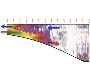
Figure 2. (a) Regime I characterises a system that hosts local, quasi-isotropic convective cells everywhere in the surface layer, while shallower waters become colder than deeper waters. This regime has a finite time window  $\tau _{t}$ whose end characterises the transition to a flow dominated by horizontal convection. (b) Regime II is characterised by the expansion of horizontal convection, from the region that experiences the largest lateral temperature gradient, i.e. zone (S). During regime II, the left front of the growing horizontal convection cell propagates towards the lateral boundary at a speed $u_{f}$, as illustrated in panel (b). (c) Regime III starts when the front of the LS-OC occupies all zone (P), and a quasi-steady circulation is achieved, at a time $\tau _{qs}=\tau _{t} + \tau _{a}$.
After the ‘transition time scale’,  $\tau _{t}$, the fluid motion is progressively dominated by horizontal density gradients. Thus, a LS-OC is expected to start from zone (S), which holds the largest cross-shore density gradient. We denote this second phase as regime II. Figure 2(b) schematises the expansion of the horizontal convective cell towards the shallowest lateral boundary due to a baroclinic adjustment. Its lateral growth occurs at a rate $u_{f}\equiv \textrm {d}\ell _{f}/\textrm {d} t$, with $\ell _{f}$ the position of the left front with respect to the position from where the expanding horizontal convection region emerges. Large-scale overturning circulation is characterised by a two-layer exchange flow, with a surface layer $h_{s}$ flowing toward the lateral boundary, whereas the bottom layer flows to the interior. Regime II takes place over a time scale $\tau _{a}$, which is the time required by the LS-OC to reach the lateral boundary, as illustrated in figure 2( $c$). After a time scale $\tau _{qs} \simeq \tau _{t}+\tau _{a}$, we expect the LS-OC to achieve a quasi-steady state, denoted as regime III.
In what follows, we derive, in dimensional form, the dynamic regimes and time scales governing the transition from one regime to another.
2.3.1. Heat budgets in the absence of net horizontal transport
We look at the heat budget for each of the three zones shown in figure 2(a). Initially, convective motions are laterally localised and vertically confined due to the presence of a physical barrier, either the bottom boundary in zones (P) and (S) or the background stratification in zone (I). In flat zones (P) and (I), convective plumes diverge laterally without any particular horizontal preference. The latter is not the case in the sloping region, where we expect that part of the vertical momentum carried down by the thermals is transformed into horizontal momentum. However, since the slopes of natural systems are usually mild,  $O(10^{-2})$, such a net transfer from vertical to horizontal momentum is rather weak. We will assume that during regime I, the net horizontal heat transport is negligible; thus, the heat balance can be approximated by
 \begin{equation} \partial_{t}T + \partial_{z}\left(wT\right) = \partial_{z}\left(\kappa\partial_{z}T\right), \end{equation}
where  $\partial _{\xi }$ denotes the partial derivative with respect to an arbitrary variable $\xi$. We express the vertical average of a function $\varphi (t,z)$ over a layer $h$ as $\langle {\varphi }\rangle _{{(\boldsymbol {\cdot })}} = h^{-1}\int _{h}\varphi (t,z)\,\textrm {{d}}z$. Here, the subscript $(\boldsymbol {\cdot })$ will indicate zone (P), (S) or (I). Thus, integrating (2.6) over the water column $d$ in zone (P), and applying the boundary conditions of the problem, i.e. $w=0$ at $z=D-d$ and $z=D$, and $\kappa \partial _{z}T=-I_{0}$ at $z=D$ and $\kappa \partial _{z}T = 0$ at $z=D-d$, we obtain
 \begin{equation} \partial_{t}\langle T\rangle_{{(P)}} ={-}\frac{I_{0}}{d} . \end{equation}
Integrating (2.7) in time, and assuming that the initial time is  $t_{0}=0$, the mean temperature in zone (P) evolves as
 \begin{equation} \langle T\rangle_{{(P)}} = \langle T(t_{0})\rangle_{{(P)}} -\frac{I_{0}}{d}t. \end{equation}
In zone (I), however, the heat budget integrates the contribution of the diffusive and advective fluxes at the base of the convective mixing layer,
 \begin{equation} \partial_{t}\langle T\rangle_{{(I)}} ={-}\frac{1}{h_{m }}\left\{I_{0}+(\kappa\partial_{z}T)\large|_{z=z_{m}} + ( w T)\large|_{z=z_{m}}\right\} , \end{equation}
where  $z_{m}$ is the height at the base of the surface mixed layer. However, vertical fluxes at the base of the convective layer can be substantially diminished by the action of the temperature jump and the intensification of the background stratification (Deardorff, Willis & Lilly Reference Deardorff, Willis and Lilly1969; D'Asaro, Winters & Lien Reference D'Asaro, Winters and Lien2002). The net heat flux at a convective layer base is about one order of magnitude smaller than the surface heat flux (Zilitinkevich Reference Zilitinkevich1991). Therefore, in order to obtain an analytical approximation of $\langle T\rangle _{(I)}(t)$, the balance in (2.9) can be simplified to
 \begin{equation} \partial_{t}\langle T\rangle_{{(I)}} \approx{-}\frac{I_{0}}{h_{m }} , \end{equation}
thus,
 \begin{equation} \langle T\rangle_{{(I)}} \approx \langle T(t_{0})\rangle_{{(I)}} -\frac{I_{0}}{h_{m}}t . \end{equation}
 In the sloping region (S) the  $x$-dependent depth-averaged temperature evolution, $\langle T\rangle _{{(S)}}$, is analogous to (2.8) and (2.11) but normalised by the local depth, $D_{B}(x)$. Note that $\langle T(t_{0})\rangle _{{(P)}}=\langle T(t_{0})\rangle _{{(S)}}=\langle T(t_{0})\rangle _{{(I)}}$.
Since we are considering that  $T>T_{MD}$, and that drops in temperature due to a cooling phase during a day are small relative to $T_{s}$ $({\sim }0.1^{\circ }\ \textrm {day}^{-1})$, a linear EoS provides a robust approximation to estimate the density, $\rho$, and buoyancy, $b$, for each zone, i.e.
 $$\begin{gather} \frac{\langle\rho\rangle_{{(\boldsymbol{\cdot})}}}{\rho_{0}}-1=\alpha\left(\langle T \rangle_{{(\boldsymbol{\cdot})}} - T_{0}\right) , \end{gather}$$
 $$\begin{gather}\langle b \rangle_{{(\boldsymbol{\cdot})}} ={-}g\left(\frac{\langle\rho\rangle_{{(\boldsymbol{\cdot})}}}{\rho_{0}}-1\right)={-} g\alpha\left(\langle T \rangle_{{(\boldsymbol{\cdot})}} - T_{0}\right) . \end{gather}$$
2.3.2. Vertical momentum balance
Now we consider the vertical momentum balance during the first regime,
 \begin{equation} \partial_{t}w + \boldsymbol{\nabla}\boldsymbol{\cdot}\left(\boldsymbol{v}w \right) ={-} \rho^{{-}1}_{0} \partial_{z}p + b + \nu\nabla^{2}w . \end{equation}
Assuming that natural convection controls the vertical momentum transport, i.e.that the advection of momentum balances buoyancy, the viscous term  $\nu \nabla ^{2}w$ can be neglected from (2.14). As we show in § 2.2, (2.5b), the diffusion of momentum, $\nu \nabla ^{2}\boldsymbol {v}$, is inversely proportional to the Rayleigh number ( $Ra$) of the system, thereby for high- $Ra$, the contribution of $\nu \nabla ^{2}\boldsymbol {v}$ becomes negligible. Therefore, averaging (2.14) between the surface $z=D$ and a height $z\geqslant D-d$, $\langle \boldsymbol {\cdot } \rangle _{{D-z}} = ({1}/({D -z}))\int ^{D}_{z} \boldsymbol {\cdot } \,\textrm {{d}}z$, and considering that variations of the vertical velocity during regime I are negligible, $\partial _{t}\langle w\rangle _{D-z}\sim 0$, the vertical momentum balance reduces to
 \begin{equation} \left.-\frac{w^{2}}{2}\right|_{z} \approx{-}\left(\frac{p_{{D}}-p}{\rho_{0}}\right) + \langle b \rangle_{{D-z}}\left(D-z\right) . \end{equation}
Here  $p_{{D}}$ and $p$ denote the pressures at the surface and a height $z$, respectively. Then, the balance in (2.15), can be expressed as
 \begin{equation} \frac{p - p_{{D}}}{\rho_{0}} ={-} \langle b \rangle_{{D-z}}\left(D-z\right)-\left.\frac{w^{2}}{2}\right|_{z} . \end{equation}
The expression (2.16) shows that the pressure  $p$ has a hydrostatic component, ${\langle b \rangle _{D-z}(D-z)}$, and a non-hydrostatic component, $w^{2}/2$.
2.3.3. Cross-shore pressure gradient
The cross-shore pressure gradient at  $z=D-d$, the depth of zone (P), increases in time due to differential cooling. From (2.16) and (2.13), we can estimate $\partial _{x}p$ directly from the cross-shore temperature gradient,
 \begin{equation} \rho^{{-}1}_{0}\partial_{x} p = dg\alpha\partial_{x}\langle T \rangle_{{D-z}} . \end{equation}
A constant sloping bottom induces a uniform pressure gradient across zone (S). Thus, recalling that  $B_{0}= -g\alpha I_{0}$, the time-dependent, cross-shore pressure gradient between zones (P) and (I) can be estimated from (2.8) and (2.11) as
 \begin{equation} \left.\rho^{{-}1}_{0}\partial_{x} p\right|_{z=D-d} \approx \frac{d g \alpha}{\ell_{s}}\left(\langle T \rangle_{{(I)}} - \langle T \rangle_{{(P)}}\right) ={-}\frac{B_{0}}{\ell_{s}}\left( 1 -\frac{d}{h_{m}}\right)t . \end{equation}
 In general, the horizontal temperature difference,  $\langle T\rangle _{{(I)}} - \langle T \rangle _{{(P)}}$, is substantially smaller than the temperature difference between the top and the bottom layer in the stratified interior region (I), $\Delta T$.
2.3.4. Cross-shore momentum balance
We examine now the cross-shore momentum balance during regime I,
 \begin{equation} \partial_{t}u + \boldsymbol{v}\boldsymbol{\cdot}\boldsymbol{\nabla}u ={-} \rho^{{-}1}_{0}\partial_{x}p + \nu\nabla^{2}u . \end{equation}
Previous works have considered a three-way linear momentum balance between the inertial, the viscous and the cross-shore pressure gradient terms to derive asymptotic solutions for the cross-shore velocity at small slopes and low- $Ra$ (Farrow & Patterson Reference Farrow and Patterson1993). Here, however, we use similar arguments to those adopted by Finnigan & Ivey (Reference Finnigan and Ivey1999) to integrate the role of advection, $\boldsymbol {v}\boldsymbol {\cdot }\boldsymbol {\nabla }u$, on the formation of a horizontal overturning due to an increase in time of the cross-shore pressure gradient. Neglecting the viscous term in (2.19), and considering that once the LS-OC starts the flow becomes largely horizontal, (2.19) reduces to the following three-way momentum balance:
 \begin{equation} \partial_{t}u + \partial_{x}\left(\frac{u^{2}}{2}\right) \approx{-} \partial_{x}\left(\frac{p}{\rho_{0}}\right) . \end{equation}
2.3.5. Transition time scale –  $\tau _{t}$

We aim at determining the time scale at which the cross-shore pressure gradient balances the inertial terms in (2.20), i.e.
 \begin{equation} -\partial_{x}\left(\frac{p}{\rho_{0}}\right) \simeq \partial_{t}u\simeq \partial_{x}\left(\frac{u^{2}}{2}\right). \end{equation}
From (2.21) and the cross-shore pressure gradient in (2.18), we derive two horizontal velocity scales,
 $$\begin{gather} \partial_{t}u\simeq{-}\partial_{x}\left(\frac{p}{\rho_{0}}\right) \quad \rightarrow\quad u\simeq \frac{B_{0}}{\ell_{s}}\left( 1 -\frac{d}{h_{m}}\right)\frac{t^{2}}{2} , \end{gather}$$
 $$\begin{gather}\partial_{x}\left(\frac{u^{2}}{2}\right)\simeq{-}\partial_{x}\left(\frac{p}{\rho_{0}}\right) \quad \rightarrow\quad u\simeq \sqrt{2B_{0}\left( 1 -\frac{d}{h_{m}}\right)t} . \end{gather}$$
The three-way balance (2.21) is achieved at a time scale  $\tau _{t}$ at which the velocity scale $u$ allows balancing the inertial terms with the cross-shore pressure gradient. Therefore, by equating expressions (2.22) and (2.23) yields
 \begin{equation} \tau_{t}\simeq \frac{2\ell_{s}}{\left(B_{0}\ell_{s}\right)^{1/3}}\left(1-\frac{d}{h_{m}}\right)^{{-}1/3} . \end{equation}
The time scale  $\tau _{t}$ defines the transition from regime I to regime II, schematised in figure 2(b), and at $\tau _{t}$, the characteristic horizontal velocity scale, $u_{t}$, is given by
 \begin{equation} u_{t}\simeq 2\left(B_{0}\ell_{s}\right)^{1/3} \left(1-\frac{d}{h_{m}}\right)^{1/3} . \end{equation}
The exchange flow associated with the LS-OC should start developing in the zone with the maximum cross-shore pressure gradient, i.e. zone (S). Considering that this zone has a uniform slope, we expect the LS-OC to emerge at about the middle of zone (S), as shown later via numerical experiments.
2.3.6. Adjustment time scale – $\tau _{a}$

We now aim to determine the time scale required by the LS-OC to reach the lateral boundary in zone (P) and be adjusted to a new equilibrium state. This adjustment time scale,  $\tau _{a}$, depends on the horizontal length of the nearshore area between the point from where the thermal siphon starts and the lateral boundary. During regime II, this nearshore area can be split into two regions, a region of length $\ell _{f}(t)$ (measured from the starting point) that grows in time due to the lateral expansion of the LS-OC and its neighbouring region that shrinks in time, where quasi-isotropic convective cells dominate the local flow, as depicted in figure 2(b). In this shrinking well-mixed zone, denoted as (LP), the average buoyancy results from the expressions (2.8) and (2.13),
 \begin{equation} \langle b \rangle_{{(LP)}} ={-}\frac{B_{0}}{d}\, t . \end{equation}
In zone (LP) the temperature and buoyancy are continuously decreasing, and  $\langle b \rangle _{{(LP)}}$ matches the buoyancy at the left front of the horizontal convective cell, $\ell _{f}(t)$. Following the arguments by Phillips (Reference Phillips1966), we assume that the momentum of the surface layer current $u_{s}$ and buoyancy are found in an inertia–buoyancy balance. This assumption implies the flow within the horizontal convective cell scales as $u_{s}\simeq (2\langle b\rangle _{{(LP)}}h_{s}) ^{1/2}$, where $h_{s}$ is the thickness of the surface exchange layer, shown in figure 2(b). Additionally, we may also consider that the surface buoyancy flux, $B_{0}$, across $\ell _{f}$ is balanced with the production of kinetic energy, which leads to the scaling velocity $u_{s}\simeq (2B_{0}\ell _{f})^{1/3}$. Hence, the above two velocity scales are equal when
 \begin{equation} \langle b \rangle_{{(LP)}} \simeq \frac{\left(2B_{0}\ell_{f}\right)^{2/3}}{2h_{s}} . \end{equation}
 By equating (2.26) and (2.27), we can derive the time scale required by the exchange flow to reach the lateral boundary. The latter is reached when  $\ell _{f}(\tau _{a})\simeq \ell _{p}+\ell _{s}/2$,
 \begin{equation} \tau_{a} \simeq \frac{d}{h_{s}}\,\frac{\ell_{f}}{\left(2\ell_{f}B_{0}\right)^{1/3}} , \end{equation}
where  $\tau _{a}$ represents the time scale needed for the LS-OC to fully adjust across zones (P) and (S). As a consequence, the time scale $\tau _{qs}\simeq \tau _{t}+\tau _{a}$ represents the time required to achieve the quasi-steady state that characterises regime III.
2.4. Numerical experiments
We examine the theoretical regimes derived in § 2.2 by means of numerical experiments. Previous studies investigated different forcing intensities for fixed basin's geometries (Horsch & Stefan Reference Horsch and Stefan1988; Bednarz et al. Reference Bednarz, Lei and Patterson2009; Mao et al. Reference Mao, Lei and Patterson2010). Here, instead, we vary the geometrical properties of the nearshore topography and keep the thermal forcing constant yet considering higher Rayleigh numbers than those examined in previous studies (Horsch & Stefan Reference Horsch and Stefan1988; Bednarz et al. Reference Bednarz, Lei and Patterson2009; Mao et al. Reference Mao, Lei and Patterson2010).
Building on the conceptual model and parameters introduced in §§ 2.1–2.2, we conducted four experiments listed in table 1. We considered three different slopes  $\bar {s}$ below 10 %, which are representative of nearshore aquatic systems like lakes and coastal seas. Also, we examined two values for $A^{(h)}$ to test the impact of the plateau extent on the time scale $\tau _{qs}$. The initial stratification characterises a strongly stratified environment as observed in late summer in temperate lakes, with a convective Richardson number $Ri_{c}\approx 10^{3}$. Our numerical experiments explore moderate thermal forcing scenarios observed in natural aquatic systems, with Rayleigh numbers $Ra\approx 10^{5}$ and $Ra_{h}\approx 10^{5}$ introduced in § 2.2, and global Rayleigh numbers $10^{18}\leqslant Ra_{g}\leqslant 10^{20}$ defined by Mao et al. (Reference Mao, Lei and Patterson2010). Thus, the magnitude of the parameters adopted for the numerical experiments are close to those found in nearshore lakes (Bouffard & Wüest Reference Bouffard and Wüest2019, and references therein), and especially similar to those in Rotsee, Switzerland (Doda et al. Reference Doda, Ramón, Ulloa, Wüest and Bouffard2021). For the parameters used in the experiments, the time scales $\tau _{t}$ and $\tau _{qs}$, are shorter than $T_{day}=24$ h.
Table 1. Non-dimensional parameters of numerical experiments and time scales associated with the transition from regime I to regime II,  $\tau _{t}$, and the transition from regime II to regime III, $\tau _{qs}$, with $T_{day}=24$ h. The ratios $\varDelta _{x,z}/(\eta _{K},\eta _{B})$ determine the global grid resolution in terms of the Kolmogorov and Batchelor scales, $\eta _{{K}}$ and $\eta _{{B}}$, respectively.

To achieve real-scale conditions, we resolved the two-dimensional version of the equations of motion (2.5) using a spectral large-eddy simulation (SLES) approach integrated in the solver flow_solve (Winters & de la Fuente Reference Winters and de la Fuente2012). The SLES approach combines a Laplacian operator with a high-order operator (‘hyper-diffusion’), which works on the temperature and the velocity fields to dissipate variance cascaded to the smallest scales near the grid spacing. This localised dissipation has a negligible effect at scales larger than a few times the grid resolution over a time scale of a few time steps (cf. Winters Reference Winters2016; Ulloa et al. Reference Ulloa, Winters, Wüest and Bouffard2020). A discussion of this approach and an explicit demonstration of the insensitivity to moderate changes in the parameters is given in Winters (Reference Winters2016). Table 1 compares the grid resolution of the numerical experiments,  $\varDelta _{x}\approx \varDelta _{z}$, to the bulk Kolmogorov and Batchelor scales of the flow, $\eta _{K}$ and $\eta _{B}$, respectively (Appendix B), which were computed a posteriori. The simulations are characterised by $\varDelta _{x,z}/\eta _{K}<10$ and $\varDelta _{x,z}/\eta _{B}\leqslant 21$. For these spatial resolutions, Gayen, Griffiths & Hughes (Reference Gayen, Griffiths and Hughes2014) classified their numerical experiments as fairly resolved LES. Appendix A describes the numerical modelling approach, whereas tables 2 and 3 present the dimensional parameters used to set the numerical experiments.
Table 2. Numerical parameters kept invariant among the numerical experiments.

Table 3. Numerical parameters that vary among the numerical experiments.

3. Numerical results
3.1. Flow patterns and geometry
The results from the simulations show the existence of the three main convective regimes. As an example, we use exp. 1 (table 1) to illustrate the spatiotemporal flow patterns by examining the cross-shore velocity component,  $u(t,\boldsymbol {x})$, and the streamfunction, $\psi (t,\boldsymbol {x})=\int ^{z}_{z_0} u(t,x,z)\, \textrm {d} z$, as shown in figure 3. Additionally, we examine the flow geometry, $F_{G}$, defined as
 \begin{equation} F_{G}(t) \equiv \frac{\sqrt{\langle u^{2}\rangle} +c}{\sqrt{\langle w^{2}\rangle}+c}. \end{equation}
The quantity  $\langle \varphi \rangle$ denotes the spatial average of a function $\varphi$ over the plateau zone (P), whereas $c\ll \sqrt {\langle u^{2}\rangle }, \sqrt {\langle w^{2}\rangle }$ is a positive constant to avoid a singularity when fluid is at rest, i.e. before the onset of RBTC. Thus, $F_{G}$ is a positive defined function of time that provides information on the global geometry of the flow in the cross-shore/vertical plane, and we use it as a diagnostic parameter to identify the transition among the different regimes. When $F_{G}\approx 1$, the flow geometry is quasi-isotropic, and as $F_{G}$ turns larger than unity, the fluid trajectory becomes more elliptic, implying that on average, horizontal motions become more dominant than vertical motions.

Figure 3. Flow patterns described by the non-dimensional horizontal velocity component,  $u/u_{t}$, and the non-dimensional streamfunction, $\tilde {\psi }=\psi /(u_{t}d)$, with $u_{t}$ the horizontal velocity scale defined in (2.25) at different non-dimensional times $t/\tau _{t}$, with $\tau _{t}$ the transition time scale in (2.24). (a,b) Instantaneous snapshot at $t/\tau _{t}=0.5$ for regime I. (c, d) Instantaneous snapshot at $t/\tau _{t}=1.5$ for regime II. (e, f) Instantaneous snapshot at $t/\tau _{t}=3.0$ for regime III. Values for $u_{t}$ and $\tau _{t}$ are provided in table 1. Movie 1 in the supplementary material available at https://doi.org/10.1017/jfm.2021.883 shows the spatiotemporal evolution of $u/u_{t}$ for exp. 1.
3.1.1. Regime I: $0< t/\tau _{t}<1$

Figure 3(a,b) shows the non-dimensional cross-shore velocity,  $u/u_{t}$, along the non-dimensional streamfunction $\tilde {\psi } = \psi /(u_{t}d)$ on the plane $x$–
$x$– $z$ at time $t/\tau _{t}=0.5$. Once convection begins, the flow pattern is organised in quasi-isotropic convective cells that occupy the whole water column in the plateau (P) and sloping (S) zones, and the mixed layer in the interior zone (I). The strength of convection is maximal in zone (I), and it decays towards the shallower zones (S) and (P), as shown in figure 3(a). In contrast, the stratified and deepest region in zone (I), $(D-z)/d>4.5$, exhibits weak but comparable flow magnitudes to those in zone (P), where convective plumes have the shortest vertical excursion, ${\sim }d$, making their convective speed the smallest one in the basin. In regime I, the fluid motion is extremely localised, and it is organised in an array of alternated clockwise and counter-clockwise circulation cells as shown by $\tilde {\psi }$ in figure 3(b).
Figure 4 shows the metric  $F_{G}$, as a function of the non-dimensional time $t/\tau _{t}$, for each experiment. Initially, and by construction, $F_{G}=1$. At the onset of RBTC, $F_{G}$ exhibits momentarily values lower than unity since it integrates mostly vertical motion (see circle A). After this event, $F_{G}$ takes values partially higher than unity due to the quasi-isotropic characteristic of the convective flow, yet it shows a gradual increase until $t/\tau _{t}\approx 1$. At this time, $F_{G}$ reaches a value close to $1.5$.

Figure 4. Flow geometry,  $F_{G}$, as a function of the non-dimensional time $t/\tau _{t}$. Values for $\tau _{t}$ are summarised in table 1. Circle A denotes the onset of RBTC. Circle B stresses the time for the transition to horizontal convection. Circle C highlights the instants when the horizontal convective cell reaches the lateral boundary, $x/\ell _{s}=0$.
3.1.2. Regime II: $1\lesssim t/\tau _{t}<\tau _{qs}/\tau _{t}$

Regime II exhibits a progressive change in the flow pattern. Figure 3(c,d) shows  $u/u_{\tau }$ and $\tilde {\psi }$, respectively, at time $t/\tau _{t}=1.5$. The transition from quasi-isotropic convective cells to a LS-OC occurs at about $t/\tau _{t}\approx 1$, when convective cells start to merge and organise in a greater elliptical cell near the upper half of the sloping zone (S), $1\leqslant x/\ell _{s}\leqslant 1.5$. Figure 3(d) shows the signature of such a process, where we identify a large counterclockwise circulation taking place across the boundary between zones (P) and (S). This circulation pattern has a distinctive two-layer exchange flow, with a bottom layer running downslope from zone (P) to zone (S) and a surface layer flowing in the reverse direction.
The structure of the exchange flow that propagates upslope is well defined, with a depth for the stagnation point stable in time. As the left front of the LS-OC propagates across zone (P), it erodes the region that is still dominated by quasi-isotropic convective cells. On the other hand, the structure of the exchange flow that propagates downslope is rather chaotic and pulsating, and its signature becomes weaker as it reaches zone (I). At the same time, an equally large but less coherent clockwise circulation is formed across zones (S) and (I),  $1.75\leqslant x/\ell _{s}\leqslant 2.25$, whereas further offshore, the flow pattern is governed by RBTC, as shown in figure 3(c,d) for $2.5\leqslant x/\ell _{s}\leqslant 3.5$.
The metric  $F_{G}$ shows a break in its trend at $t/\tau _{t}\approx 1$, as shown on the highlighted circle B in figure 4. We associate this break with the expansion of horizontal convection that characterises regime II. Indeed, $F_{G}$ experiences a remarkable increase in its growth rate due to the shift from quasi-isotropic convective cells to the LS-OC that occurs across zones (S) and (P). As time progresses, however, $F_{G}$ starts to reduce its growth ( $t/\tau _{t}>2$) in a way that the curves begin to converge and oscillate around a value of $F_{G}\approx 5$, indicating that fluid motion in zone (P) is predominantly horizontal.
From the results in figure 4, the time associated with the shift from regime II to regime III is not evident. However, circle C highlights a marked change in  $F_{G}$ that allows identifying the emergence of a new dynamic regime. We found that the oscillatory signal that starts at $t/\tau _{t}\approx 1.8$ for exp. 4 occurs when the left front of the LS-OC reaches the lateral boundary, $x/\ell _{s}=0$. After this time, $F_{G}(t)$ oscillates around $F_{G}\approx 5$. To estimate the time scale associated with the transition from regime II to regime III, $\tau _{qs}\simeq \tau _{t}+\tau _{a}$, we require the thickness of the surface exchange layer $h_{s}$, depicted in figure 2(b), which is so far unknown. However, both $\tau _{qs}$ and $h_{s}$ can be obtained from the numerical experiments.
We first estimate the time  $\tau ^{(exp)}_{qs}$ at which the left front reaches the lateral boundary $x/\ell _{s}=0$. For this, we look at the evolution of the near-surface, cross-shore velocity, defined by convenience as
 \begin{equation} \bar{u}_{s}(t,x)\equiv \frac{1}{d/3}\int^{D}_{D-d/3} u(t,x,z) \, \textrm{d}z . \end{equation}
Knowing that the upper layer velocity of the LS-OC has a negative sign and propagates towards the shore ( $x/\ell _{s}=0$), its left front is easy to track by examining $\bar {u}_{s}$.
Figure 5 shows  $\bar {u}_{s}(t,x)/u_{t}$ (colour map) for each experiment. The horizontal axes denote the non-dimensional position $x/\ell _{s}$ whereas the vertical axes denote the non-dimensional time $t/\tau _{t}$. Blue colours denote on-shore currents, while red colours denote off-shore currents. Thus, the evolution of the blue region is associated with the irreversible expansion of the LS-OC that starts approximately about $t/\tau _{t}\simeq 1$, in the middle of zone (S). In particular, the left diagonal boundary of the large blue region denotes the spatiotemporal position of the front, and its intersection with the vertical axis at $x/\ell _{s}=0$ (marked by a green circle) allows for estimating $\tau ^{(exp)}_{qs}$.

Figure 5. Near-surface cross-shore velocity,  $\bar {u}_{s}(t,x)$, normalised by $u_{t}$ as a function of cross-shore position $x/\ell _{s}$ and time $t/\tau _{t}$ for (a) exp. 1, (b) exp. 2, (c) exp. 4 and (d) exp. 3 (see table 1). Note that exp. 1 and exp. 4 have been placed one on top of the other for easier visual comparison. Each map is divided in nine regions. Across the space coordinate $x/\ell _{s}$, we distinguish: the plateau zone (P), between $x/\ell _{s}=0$ and the left vertical dashed line; the sloping zone (S), between the two vertical dashed lines; and the interior zone (I), between the right vertical dashed line and $x/\ell _{s}=3.5$. On the time coordinate $t/\tau _{t}$, we identify: the theoretical regime I, $0< t/\tau _{t}\lesssim 1$, followed by the regime II, between $t/\tau _{t}\simeq 1$ and the time when the left front of the exchange flow reaches $x/\ell _{s}=0.0$, marked by a green circle on the vertical axis. This time is denoted as $\tau ^{(exp)}_{qs}$. Regime III is characterised by times $t/\tau _{t}$ above the upper horizontal dashed line.
The empirical estimation of  $\tau _{qs}$ allows for examining the adjustment time scale $\tau _{a}$ (2.28), which depends on the characteristic thickness of the upper exchange layer, $h_{s}$. Figure 3(e) provides a spatial view of $u/u_{t}$, and shows that $h_{s}$ varies little across zone (P). In figure 6 we provide a detailed view of the cross-shore velocity profile $u/u_{t}$ at the middle of zone (P). Green lines in figure 6 show the time-averaged velocity profile over regime I, $\bar {u}_{{R1}}/u_{t}$. Its maximum magnitude, $\bar {u}_{{R1}}/u_{t}\sim O(0.1)$, and vertical distribution results from time averaging a flow dominated by localised, quasi-isotropic convective cells. Red lines show the time-averaged velocity profile over regime II, $\bar {u}_{{R2}}/u_{t}$. To obtain $\bar {u}_{{R2}}/u_{t}$, we followed two steps. We first used $\tau ^{(exp)}_{qs}$ (estimated from figure 5) to examine the vertical structure of the time-averaged velocity profile over $t\in [\tau _{t},\tau ^{(exp)}_{qs}]$. From this velocity profile, we found that $h^{(exp)}_{s}/d\approx 0.35$ for all the experiments. We then used the experimental value of $h^{({\rm exp})}_{s}$ to re-estimate $\tau _{a}$ and $\tau _{qs}\simeq \tau _{t}+\tau _{a}(h^{(exp)}_{s})$ from the theoretical expressions (2.24) and (2.28). Thus, $\bar {u}_{{R2}}/u_{t}$ in figure 6 results from a time averaging over $t\in [\tau _{t},\tau _{qs}(h^{(exp)}_{s})]$. We use then $\tau _{qs}$ to normalise the evolution in time of $F_{G}$, as shown in figure 7. In this new non-dimensional time, all the curves of $F_{G}$ collapse after $t/\tau _{qs}=1$, which defines the end of regime II and the beginning of regime III.

Figure 6. Non-dimensional cross-shore velocity component,  $u/u_{t}$, at the middle point $x_{*}$ of zone (P). (a) Exp. 1, $x/\ell _{s}=0.5$. (b) Exp. 2, $x/\ell _{s}=0.5$. (c) Exp. 3, $x/\ell _{s}=0.5$. (d) Exp. 4, $x/\ell _{s}=0.25$. Note that exp. 1 and exp. 4 have been placed one on top of the other for easier visual comparison. Grey lines show the superimposed velocity profiles of $u$ over the three regimes. Green lines show the time-averaged velocity profile, $\bar {u}_{{R1}}$, over regime I. Red lines show the time-averaged velocity profile, $\bar {u}_{{R2}}$, over regime II. Blue lines show the time-averaged velocity profile, $\bar {u}_{{R3}}$, over regime III. The horizontal dashed line denotes $(D-z)/d = 0.35$.

Figure 7. Flow geometry,  $F_{G}$, as a function of the non-dimensional time $t/\tau _{qs}$. Values for $\tau _{qs}$ are summarised in table 1.
3.1.3. Regime III: $1\lesssim t/\tau _{qs}$

Figure 3(e, f) shows  $u/u_{t}$ and $\tilde {\psi }$, respectively, at time $t/\tau _{t}=3.0$. In regime III convection takes the form of a counter-clockwise LS-OC across zones (P) and (S). Blue lines in figure 6 show the time-averaged velocity profile over regime III, $\bar {u}_{{R3}}/u_{t}$. Note that the magnitude of $\bar {u}_{{R3}}/u_{t}$ is larger than the magnitude of $\bar {u}_{{R2}}/u_{t}$ since regime II integrates the transition from localised, quasi-isotropic convective cells to a full LS-OC across zone (P).
The well-defined exchange flow observed along zone (P) and the upper zone (S) differs from the complex flow that characterises the pass from zone (S) to (I), shown in figure 3( f) ( $1.75\leqslant x/\ell _{s}\leqslant 2.25$). In this transition region, convective plumes are energetic enough to erode the weak stratified flow induced by the LS-OC and act as a lateral obstacle that holds the LS-OC in the shallower zones. In zone (I) the flow structure exhibits prominent localised convective cells, which are wider and more unstable than those observed early in regime I. The latter may be the signature of the unsteady flows developed in the deeper zone (S) and the remnants of the transient flow experienced in regime II. The unsteadiness generated in the deeper zone (S) may also propagate upslope. As an example, figure 5(c) highlights pulsating signals in $\bar {u}_{s}$. The pulses are characterised by diagonal white stripes crossing the broad blue region, showing that they propagate from zone (S) towards zone (P). This pulsating feature in the flow is also imprinted in $F_{G}$, as shown in figure 7, for $t/\tau _{qs}\geqslant 1$.
3.2. Cross-shore transport
The development of the LS-OC boosts the cross-shore transport,  $\mathcal {Q}_{{Exp}}$. Here, we quantify $\mathcal {Q}_{{Exp}}(t)$ at the boundary between zones (P) and (S), where a two-layer exchange flow is well defined,
 \begin{equation} \mathcal{Q}_{{Exp}}(t) \equiv \tfrac{1}{2}\int^{D}_{D-d} |u(t,x=\ell_{p},z)|\, \textrm{d}z . \end{equation}
In the quasi-steady state the cross-shore transport can be estimated from Phillips (Reference Phillips1966) velocity scale,  $(B_{0}\ell _{p})^{1/3}$, and the local depth, $d$, as
 \begin{equation} \mathcal{Q}_{qs}\simeq \mathcal{A} d\left(B_{0}\ell_{p}\right)^{1/3} , \end{equation}
where  $\mathcal {A}$ is a constant coefficient to be determined. For the conditions in regime III, we compute for each experiment $\mathcal {Q}_{{Exp}}(t)$ and the respective time-averaged coefficient $\mathcal {A}$,
 \begin{equation} \bar{\mathcal{A}}_{{Exp}} = \frac{1}{d \left(B_{0}\ell_{p}\right)^{1/3}}\left\{ \frac{1}{\tau_{m}-\tau_{qs}}\int^{\tau_{m}}_{\tau_{qs}} Q_{{Exp}}(t) \, \textrm{d} t\right\}. \end{equation}
 Figure 8 shows the time series of  $\mathcal {Q}_{{Exp}}(t)$ for each experiment, normalised by their respective scaling $\mathcal {Q}_{qs}$, with $\bar {\mathcal {A}}=(1/4)\sum ^{4}_{i=1}\bar {\mathcal {A}}_{{Exp\,i}}=0.35 \pm 0.05$. The time-averaged values $\bar {\mathcal {A}}_{{Exp\,i}}$, along with their standard deviations, are summarised in the legend of figure 8. The time axis in figure 8 is normalised by $\tau _{qs}$, which allows stressing the transition between regimes II to III at $t/\tau _{qs}\simeq 1$. In this non-dimensional time, the time series of $\mathcal {Q}_{{Exp}}(t)/\mathcal {Q}_{qs}$ show a first transient phase over which the magnitude of the cross-shore transport has significant variability as well as a progressive increase. Not surprisingly, $\mathcal {Q}_{{Exp}}(t)/\mathcal {Q}_{qs}$ shows a stabilisation before $t/\tau _{qs}=1$. The latter is due to the fact that at the location where we measure $Q_{{Exp}}(t)$, the horizontal exchange flow forms earlier than the time $\tau _{qs}$ required to reach the lateral boundary. For times $t/\tau _{qs}\geqslant 1$, the results show a quasi-steady cross-shore transport, with a standard deviation $\sigma$ of about $15\,\%$ over its mean value. Thus, for the set of parameters considered in the numerical experiments, the scaling $\mathcal {Q}_{qs}\simeq 0.35d(B_{0}\ell _{p})^{1/3}$ is a robust predictor of the cross-shore transport between zones (P) and (S) under quasi-steady-state conditions.

Figure 8. Experimental cross-shore transport  $\mathcal {Q}_{{Exp}}(t)$ scaled by $\mathcal {Q}_{qs}=\bar {\mathcal {A}}\,d(B_{0} \ell _{p})^{1/3}$, with $\bar {\mathcal {A}}=0.35\pm 0.05$.
3.3. Evolution of the cross-shore thermal field
Figure 9 shows the spatiotemporal evolution of the non-dimensional temperature field  $(T-T_{b})/\Delta T$ for exp. 1. Zone (P) has the coolest temperature above the thermocline height, whereas the convective mixing layer in zone (I) is the warmest region.

Figure 9. Spatiotemporal evolution of the relative temperature field  $(T-T_{b})/\Delta T$. Zone (P): $0\leqslant x/\ell _{s}\leqslant 1$; zone (S): $1\leqslant x/\ell _{s}\leqslant 2$; zone (I): $2\leqslant x/\ell _{s}\leqslant 3.5$. Movie 2 in the supplementary material shows the spatiotemporal evolution of $(T-T_{b})/\Delta T$ for exp. 1.
During regime I ( $0\leqslant t/\tau _{t}< 1.0$), waters above the thermocline remain vertically well mixed due to turbulent convection. Zones (P) and (I) also remain horizontally mixed. As time progresses, a cross-shore temperature difference builds up between zones (P) and (I), where the maximum horizontal temperature gradient is found across zone (S) ( $1.0\leqslant x/\ell _{s}\leqslant 2.0$), as shown in figure 9(a). However, we identify that at about $t/\tau _{t}\simeq 1.0$ warmer waters entrain above colder waters in zone (P) ( $x/\ell _{s}\approx 1.5$), as shown in figure 9(b). This localised overturn is associated with the development of the overturning circulation that characterise regime II.
Figure 9(c–e) shows the thermal structure resulting from the growing LS-OC during regime II. In this phase we observe the formation of a layer of cold water flowing downslope from the upper region of zone (S). At the same time, a surface layer formed by warmer waters coming from zone (S) penetrates across zone (P). Once the LS-OC is fully developed across zone (P), i.e. when regime III starts, the water column exhibits an almost uniform temperature profile towards the lateral boundary,  $x/ \ell _{s}\rightarrow 0$, and towards the end of zone (S), $x/\ell _{s} \simeq 2.0$, as shown in figure 9( f). Within this region, the exchange flow keeps waters weakly stratified and feeds a gravity current that propagates downslope. Yet, as the gravity current crosses zone (S) and approaches zone (I), its signature becomes substantially weaker and intermittent while convective plumes get more vigorous, enhancing vertical mixing and supporting the degeneration of the exchange flow. In the previous subsections we used the velocity field properties to show that the formation of the LS-OC agrees well with the transition time scale, $\tau _{t}$, in (2.24). However, for practical reasons, one might wish to infer the conditions that support forming a thermal siphon in an aquatic system by measuring the temperature at specific locations. Theoretically, the dynamic balance that controls the formation of the thermal siphon (§ 2.3.4) has a specific cross-shore temperature gradient to fulfil. In our framework, expressions (2.8) and (2.11) allow for determining the mean temperature difference and thermal gradient between zones (P) and (I) at the transition time scale $t=\tau _{t}$,
 $$\begin{gather} \varDelta\langle T\rangle_{{(IP)}} = \langle T\rangle_{{(I)}} - \langle T\rangle_{{(P)}} \approx \frac{I_{0}}{d}\left(1 - \frac{d}{h_{m}}\right)\tau_{t} , \end{gather}$$
 $$\begin{gather}\partial _{x}\langle T\rangle_{{(IP)}} = \frac{\langle T\rangle_{{(I)}} - \langle T\rangle_{{(P)}}}{\ell_{s}} \approx \frac{I_{0}}{d \ell_{s}}\left(1 - \frac{d}{h_{m}}\right)\tau_{t} , \end{gather}$$
respectively. Both expressions depend only on the geometrical properties of the nearshore basin and the kinematic heat flux  $I_{0}$. Therefore, they can be readily used to determine the mean temperature difference between the shallow and interior waters, or the mean cross-shore temperature gradient, that supports the formation of a LS-OC in a waterbody.
Note that  $\langle T\rangle _{{(P)}}$ is higher than the temperature of the deeper layer, $T_{b}$, which means that the lower branch of LS-OC can not plunge into the deeper layer of the interior basin.
We tested the ability of expression (3.6a) to predict the temperature difference between shallow and interior waters at  $\tau _{t}$. For this, we computed times series of $\varDelta \langle T\rangle _{{(IP)}}(t)$, and we scaled them by their respective temperature difference predicted in (3.6a). Figure 10 shows $[\varDelta \langle T\rangle _{{(IP)}}(t)]_{exp}/\varDelta \langle T\rangle _{{(IP)}}(\tau _{t})$ as a function of the non-dimensional time $t/\tau _{t}$. The dashed line bisecting the map represents the theoretical linear trend expected during regime I ( $0 < t/\tau _{t}<1$). Thus, for a perfect agreement, the curves should cross the coordinate (1,1). Indeed, the experimental temperature difference $[\varDelta \langle T\rangle _{{(IP)}}]_{exp}$ at $\tau _{t}$ shows values of about 90 % of the theoretically predicted.

Figure 10. Relative temperature difference between the shallow and interior waters as a function of time. Capital letters (A), (B) and (C) are associated with capital letters in figure 11.
Recalling the hypotheses adopted to derive (3.6a), i.e.no horizontal heat exchange and that the mean temperature in zone (I) is dominated by the surface heat flux, our numerical results show that these assumptions are met reasonably well, and the level of disagreement is expected. Figure 11(a) shows a close-up view of the temperature field overlapped by the velocity field in zone (S) for exp. 1 at  $t/\tau _{t}=1$. The temperature field is still almost vertically mixed, and the flow field is organised in localised convective cells, suggesting that no exchange between zones (P) and (I) takes place yet.

Figure 11. Relative temperature field  $(T-T_{b})/\Delta T$ within zone (S), $1\leqslant x/\ell _{s}\leqslant 2$, superposed by the velocity field (black arrows) for (a) $t/\tau _{t}=1.0$, (b) $t/\tau _{t}=1.3$ and (c) $t/\tau _{t}=3.0$. Capital letters (A), (B) and (C) are associated with capital letters in figure 10.
For  $t/\tau _{t}>1$, nonetheless, the curves $[\varDelta \langle T\rangle _{{(IP)}}(t)]_{exp}/\varDelta \langle T\rangle _{{(IP)}}(\tau _{t})$ start departing progressively from the dashed line due to the horizontal heat exchange that takes place across zone (S). Thus, the analytical expression (3.6a) grants a conservative estimation of the temperature difference between shallow and interior waters required to drive the LS-OC across the sloping region. However, to generate an effective heat exchange between zone (P) and the interior zone (I), the fluid within each extreme zone must first be transported all through zone (S). Therefore, we anticipate that the collapse of the curves should hold until the heat exchange driven by the LS-OC starts to influence the mean temperatures in zones (P) and (I). Indeed, we observe in figure 10 that this horizontal heat exchange becomes distinctive at about $t/\tau _{t} \gtrsim 1.3$. As an example, figure 11(b) illustrates that in exp. 1 at $t/\tau _{t}=1.3$, the heat exchange is already occurring between zones (P) and (S). After the above experimental time, the curves $[\varDelta \langle T\rangle _{{(IP)}}(t)]_{exp}/\varDelta \langle T\rangle _{{(IP)}}(\tau _{t})$ start to depart from each other and the non-dimensional temperature difference between (P) and (I) starts to grow at a slower rate due to the horizontal heat exchange throughout zone (S), as shown in figure 11(c).
4. Discussion
4.1. Relevance and scopes
Overturning circulation resulting from the uniform cooling of the surface in sloping water basins can be a persistent mode of motion in littoral aquatic environments (Doda et al. Reference Doda, Ramón, Ulloa, Wüest and Bouffard2021). This convective process, aka thermal siphon (Monismith et al. Reference Monismith, Imberger and Morison1990), is an efficient mechanism for renewing and exchanging heat and mass between shallow and deep waters (e.g. Fer et al. Reference Fer, Lemmin and Thorpe2002; Monismith et al. Reference Monismith, Genin, Reidenbach, Yahel and Koseff2006; Molina et al. Reference Molina, Pawlak, Wells, Monismith and Merrifield2014). In lakes at mid-latitudes, thermal siphons may occur during summer due to nighttime surface cooling or more continuously over autumn and winter due to the seasonal cooling (Fer et al. Reference Fer, Lemmin and Thorpe2002; Doda et al. Reference Doda, Ramón, Ulloa, Wüest and Bouffard2021), which may support the formation of deep stratification (Wells, Griffiths & Turner Reference Wells, Griffiths and Turner1999; Wells & Sherman Reference Wells and Sherman2001). From the viewpoint of the aquatic ecosystem, the robust characterisation of thermal siphons is relevant to assess their impact on diurnal and seasonal biogeochemical cycles occurring in nearshore and open waters (MacIntyre & Melack Reference MacIntyre and Melack1995; Hofmann Reference Hofmann2013; Encinas Fernández, Peeters & Hofmann Reference Encinas Fernández, Peeters and Hofmann2016; Brothers et al. Reference Brothers, Kazanjian, Köhler, Scharfenberger and Hilt2017; Donis et al. Reference Donis, Flury, Stöckli, Spangenberg, Vachon and McGinnis2017; DelSontro, del Giorgio & Prairie Reference DelSontro, del Giorgio and Prairie2017; Razlutskij et al. Reference Razlutskij, Buseva, Feniova and Semenchenko2021; Krishna et al. Reference Krishna, Ulloa, Kerimoglu, Minaudo, Anneville and Wüest2021).
In this work we characterise the formation of thermal siphons based on a three-way, cross-shore momentum balance, in which the thermally controlled pressure gradient balances the inertial terms. From this dynamic regime, we derived the first relevant scale, denoted as the transition time scale,  $\tau _{t}$ (§ 2.3.5), that is analogous to the time scale derived by Finnigan & Ivey (Reference Finnigan and Ivey1999) to characterise the emergence of the buoyancy-driven exchange flow above a sill that separates two basins of the same depth. Here, $\tau _{t}$ determines the time scale needed by the convective flow to start forming a LS-OC across the nearshore sloping waters. We characterised a third dynamic regime, in which the cross-shore pressure gradient balances the advective acceleration under steady state. From the latter balance, we derived a second time scale, denoted as $\tau _{qs}$ (§ 2.3.6), that describes the shift to a quasi-steady flow regime. For times longer than $\tau _{qs}$, a horizontal overturning occupies the nearshore basin whose depth is shallower than the base of the thermocline region in the interior waters, as shown in figures 2(c) and 3(e, f). Further offshore, Rayleigh–Bénard type convection dominates the flow structure and constrains the expansion of the nearshore, overturning circulation.
The theoretical flow regimes and time scales derived in this study are supported by numerical experiments designed to examine real-scale water basins. Our numerical tests achieved high Rayleigh numbers ( $Ra=10^{5}$, $Ra_{h}=10^{14}$, $Ra_{g}=10^{20}$, §§ 2.3.1–2.4), and simulated systems with slopes below 10 % (table 1), which is a usual scenario of aquatic systems like lakes and coastal seas. Thus, our results complement previous numerical and experimental studies that have examined basins with slopes of about 10 % or higher (Horsch & Stefan Reference Horsch and Stefan1988; Sturman et al. Reference Sturman, Oldham and Ivey1999; Wells & Sherman Reference Wells and Sherman2001; Bednarz et al. Reference Bednarz, Lei and Patterson2008, Reference Bednarz, Lei and Patterson2009; Mao et al. Reference Mao, Lei and Patterson2010). Although the theoretical time scales $\tau _{t}$ and $\tau _{qs}$ agree well with numerical experiments, they do not provide information about the dynamics governing the flow structure in the transition region between the sloping zone (S) and the interior convective mixing layer (I). Thus, future studies might focus on the fluid dynamics of this transition region to understand better how the problem's parameters and the convective regime taking place in the interior constrains the extent of the nearshore, overturning circulation.
To resolve both large-scale convective processes of about 100 m in the horizontal and about 10 m in the vertical, and small-scale processes associated with secondary instabilities and boundary layers of about centimetres, we integrated the two-dimensional equations of motions using a SLES approach implemented in the solver flow_solve (Winters & de la Fuente Reference Winters and de la Fuente2012; Winters Reference Winters2016; Ulloa et al. Reference Ulloa, Winters, Wüest and Bouffard2020). The experiments were run for a time scale of a day with a time resolution of 0.15 s. Certainly, resolving the same range of scales in a three-dimensional system, or increasing the spatial resolution to resolve Kolmogorov and Batchelor scales, will require substantially more computational resources. However, we emphasise the need to investigate further the differences and similarities between two-dimensional and three-dimensional Rayleigh–Bénard convective flows for systems with aspect ratios  $D/\mathcal {L}\ll 1$ in a similar fashion as done by van der Poel, Stevens & Lohse (Reference van der Poel, Stevens and Lohse2013) for ${D/\mathcal {L}= 1}$, with $D$ and $\mathcal {L}$ the vertical and horizontal length-scale of the water basin, respectively.
4.2. Cross-shore transport
From the numerical experiments, and Phillips (Reference Phillips1966) velocity scale,  $(B_{0}\ell _{p})^{1/3}$, we derived a semi-empirical scaling for the cross-shore transport in the shelf zone (P), $\mathcal {Q}_{qs}\simeq \mathcal {A}d(B_{0}\ell _{p})^{1/3}$, with $\mathcal {A}=0.35\pm 0.05$ (§ 3.2). If we consider the mean coefficient $\mathcal {A}\approx 0.35$, $\mathcal {Q}_{qs}$ matches the theoretical expression for estimating the maximal exchange flow above a sill that separates two basins (Farmer & Armi Reference Farmer and Armi1986; Finnigan & Ivey Reference Finnigan and Ivey2000). The above value differs partially from the coefficient obtained by Harashima & Watanabe (Reference Harashima and Watanabe1986), $0.15 \leqslant \mathcal {A}\leqslant 0.33$, and by Sturman & Ivey (Reference Sturman and Ivey1998), $\mathcal {A}\approx 0.2$, via laboratory experiments in a basin with similar geometry (shelf/slope basin) but with different boundary conditions. In the experiments conducted by Harashima & Watanabe (Reference Harashima and Watanabe1986), they imposed a destabilising heat flux on an open shallow water shelf joined with a deeper reservoir, ( $\ell _{s}=0$ or $\bar {s}\rightarrow \infty$). In this system they found that the coefficient $\mathcal {A}$ depends monotonically on the flux Reynolds number, defined as $Re_{f}\equiv (d/\ell _{p})^{2/3}(B_{0}d)^{1/3}d/\nu$, over the range $Re_{f}\sim O(10)\text {--}O(10^{2})$. In our experiments, $Re_{f} \sim O(10^{2})$, and for this magnitude, Harashima & Watanabe (Reference Harashima and Watanabe1986) obtained $\mathcal {A}\approx 0.33$, which is close to the coefficient found in the present study. In the case of Sturman & Ivey (Reference Sturman and Ivey1998), the authors imposed a solid boundary condition at the surface where we prescribed a free-slip condition, and their flux Reynolds number was about $Re_{f}\approx 40$. Indeed, the existence of an additional boundary layer (at the surface) and lower forcing conditions may have led to a reduction of $\mathcal {A}$.
Sturman & Ivey (Reference Sturman and Ivey1998) also considered a different thermal forcing scenario to investigate the cross-shore transport. They applied a surface buoyancy flux only over the shelf region (see figure 1 in Sturman & Ivey Reference Sturman and Ivey1998), which would be analogous to restricting the surface cooling to zone (P) in our system. This second difference might be more relevant for the flow developed across the sloping zone and the interior. The authors observed a well-defined downslope exchange flow able to penetrate through the interior deeper basin and whose surface was not subjected to a destabilising surface buoyancy flux. In contrast, our experiments show that the downslope gravity current is strongly degenerated and diminished as it approaches the interior deeper zone, where the surface cooling supports a vigorous RBTC. Examining the degeneration of gravity currents in convective environments requires, without a doubt, thorough investigation.
4.3. Thermal siphon and other processes
The dynamics of the thermal siphon found in this study may be affected by several processes occurring in natural waters. First, wind can act at the same time as surface cooling. Coupling both processes may indeed modify the cross-shore exchange flow properties (Farrow Reference Farrow2012; Horwitz & Lentz Reference Horwitz and Lentz2014; Ramón et al. Reference Ramón, Ulloa, Doda and Bouffard2021). Ramón et al. (Reference Ramón, Ulloa, Doda and Bouffard2021) showed that in small water basins forced by surface cooling and steady winds, the coupling effect weakens the cross-shore transport on the upwind side of the basin and boosts the cross-shore transport on the downwind side of the basins. Second, thermal siphons associated with low Rossby numbers may modify their horizontal trajectory and reduce the effective cross-shore transport in a similar fashion as shown by Cenedese et al. (Reference Cenedese, Whitehead, Ascarelli and Ohiwa2004) and by Ramón et al. (Reference Ramón, Ulloa, Doda, Winters and Bouffard2021) in radiatively heated ice-covered basins. Third, aquatic systems may experience spatial and temporal changes in the surface heat flux. In the case of small basins, spatial variability might be at first order negligible, yet the variation in time of  $B_{0}$ can be significant, especially during the summer season. One aspect to consider is that the surface layer may tend to weakly stratify during daytime due to the incoming solar radiation. The latter means that early in the cooling phase, convection has to initially mix the surface layer to fulfil the conceptual model shown in figure 1 (Doda et al. Reference Doda, Ramón, Ulloa, Wüest and Bouffard2021). Fourth, thermal siphons may interact and be modified by alongshore and cross-shore currents resulting, for instance, from large-scale oscillations, among others (Ulloa et al. Reference Ulloa, Davis, Monismith and Pawlak2018). In enclosed waterbodies like lakes, each of the aspects mentioned earlier requires particular attention.
4.4. Development of thermal siphons and non-dimensional numbers
The transition time scale  $\tau _{t}$ (2.24) can be expressed compactly as
 \begin{equation} \tau_{t} \simeq \tau_{m} G_{b}\, Ra^{{-}1} , \end{equation}
with  $\tau _{m}=2h'^{2}_{m}/\kappa$ a diffusive time scale, $Ra$ the Rayleigh number introduced in (2.2a–c) and $G_{b} = \bar {s}^{-2/3} (1-A^{(v)})^{-1/3}$ a geometrical parameter of the basin. Expression (4.1) shows that $\tau _{t}$ is inversely proportional to $Ra$, and proportional to $G_{b}$ implying that stronger surface cooling, steeper slopes $\bar {s}$ and a smaller ratio $A^{(v)}$ will shorten $\tau _{t}$ and speed up the development of thermal siphons. Here, we show the significant role of the slope in $\tau _{t}$ via experiments 1–3 (table 1), which was varied $0.03\leqslant \bar {s}\leqslant 0.09$, while keeping constant $Ra = 10^{5}$ and $A_{v}=0.2$. For this range of $\bar {s}$, $\tau _{t}$ reduced from 7.9 h to 3.8 h. These time scales are shorter than a usual cooling phase of a day, which is primarily but not exclusively associated with nighttime.
Additionally, note that the parameter  $A^{(h)}=\ell _{p}/\ell _{s}$ is not relevant to determine $\tau _{t}$, which means that the length of the shelf zone $\ell _{p}$ does not affect $\tau _{t}$ as long as the shelf's depth is fairly uniform. The latter is supported by the results in exp. 1 and exp. 4, which have the same characteristic slopes, $\bar {s}\approx 3\,\%$, but different parameters $A^{(h)}=\ell _{p}/\ell _{s}$, $A^{(h)}\approx 1.0$ and $A^{(h)}\approx 0.5$, respectively (table 1). Since $\ell _{s}$ is also the same for both experiments, the contrast rises on the time scale $\tau _{qs}$, which depends on $\ell _{p}$. Thus, in exp. 4, $\tau _{qs}$ is shorter than in exp. 1 because its shelf's length $\ell _{p}$ is shorter.
In order to gain sensibility with the magnitude of the geometrical parameters needed to compute  $\tau _{t}$, we used the bathymetric information available in sites where thermal siphons have been reported. Figure 12(a) illustrates $G_{b}$ in terms of $\bar {s}$ and $A^{(v)}$; $\bar {s}$ varies between $10^{-3}$ and values above $10^{-1}$, whereas $A^{(v)}$ varies between $10^{-2}$ and 1. For the above values, $G_{b}$ ranges between 1 and 100. Figure 12(a) also shows that, for $A^{(v)}<0.1$, the term $(1-A^{(v)})^{-1/3}$ in $G_{b}$ becomes a small correction.

Figure 12. (a) Example of the range of values for the non-dimensional parameters  $\bar {s}$ and $A^{(v)}$ observed in lakes, reservoirs and coastal seas. (b) Transition time scale $\tau _{t}$ normalised by the diffusive time scale $\tau _{m}= 2h'^{2}_{m}/\kappa$ as a function of the Rayleigh number $Ra$ and the geometrical parameter mapped in panel (a). Legend: $\circ$ Lake Anna (USA): 0.7–5.8 h (Adams & Wells Reference Adams and Wells1984); $\square$ Wellington reservoir (Australia): 0.3–2.6 h (Monismith et al. Reference Monismith, Imberger and Morison1990); $\triangledown$ Lake Banyoles (Spain): 1.3–21.8 h (Roget et al. Reference Roget, Colomer, Casamitjana and Llebot1993); $\triangleright$ Lake Victoria (East Africa): 13.1–29.2 h (MacIntyre, Romero & Kling Reference MacIntyre, Romero and Kling2002); $\diamond$ Lake Geneva (Switzerland/France): 18.5–26.1 h (Fer et al. Reference Fer, Lemmin and Thorpe2002); $\triangleleft$ Kilo Nalu (Hawaii): 4.6–5.8 h (Molina et al. Reference Molina, Pawlak, Wells, Monismith and Merrifield2014); $\bigstar$ Lake Rotsee (Switzerland) 2.6–21.2 h (Doda et al. Reference Doda, Ramón, Ulloa, Wüest and Bouffard2021).
Figure 12(b) shows the transition time scale  $\tau _{t}$ normalised by the diffusive time scale, $\tau _{t}/\tau _{m}$, as a function of $G_{b}$ (over the range obtained from figure 12a) and the Rayleigh number $Ra$ defined in (2.2a–c). Field observations show that $Ra$ may vary by two orders of magnitude, between $10^{4}$ and $10^{7}$, whereas $G_{b}$ may vary by one order of magnitude. For the above parameters’ intervals, $\tau _{t}$ can vary from tens of minutes to one day, approximately. To sum up, the expression (4.1) and figure 12 allow for: (1) a straightforward interpretation of the effect of the crucial non-dimensional parameters involved in the development of thermal siphons, and (2) estimating the transition time scale from the non-dimensional parameters and time scale $\tau _{m}$.
4.5. Application: field-scale experiments
To estimate the time scales and the cross-shore transport that characterise the thermal siphon in a specific system, we require the geometry of the nearshore basin and the surface buoyancy flux. The geometrical parameters include the characteristic length and depth of the shelf region, the characteristic slope and the depth of the surface mixed layer in the open waters ( $\ell _{p}$, $\ell _{s}$, $d$,
$d$,  $\bar {s}$, $h_{m}$). The surface buoyancy flux, $B_{0}=\alpha g H_{0}/(\rho _{0}c_{p})$, is estimated from the surface heat flux, $H_{0}$ (not considering solar radiation), and the surface waters temperature, implicitly used to determine the thermal expansivity, $\alpha$.
We illustrate the applicability of the scaling introduced in this manuscript by testing them against observations in Rotsee, Switzerland. In this lake, Doda et al. (Reference Doda, Ramón, Ulloa, Wüest and Bouffard2021) carried out a year-long field study to characterise the properties of thermal siphons induced by surface cooling. Figure 13(a,b) shows the bathymetry of Rotsee and the cross-shore topography of the study site, from where we extract the geometrical properties to estimate  $\tau _{t}$, $\tau _{qs}$ and $\mathcal {Q}_{qs}$, assuming that $h_{s}/d = 0.35$. Here, we examine two wind-free days, one in summer (02–03 August 2019) and one in autumn (5–6 October 2019). The thickness of the surface mixed layer $h_{m}$ was determined from a high-resolution thermistor chain located in the interior basin (Doda et al. Reference Doda, Ramón, Ulloa, Wüest and Bouffard2021), with $\bar {h}_{m}\approx 4.6$ m for the summer day and $\bar {h}_{m}\approx 7.2$ m for the autumn day. Zone (P) has a length of $\ell _{p}\approx 140$ m and a characteristic depth of $d\approx 1$ m. From $\bar {h}_{m}$ we determine the horizontal length of the sloping zone (S), which is $\ell _{s} \approx 110$ m for the summer day and $\ell _{s} \approx 195$ m for the autumn day. For both periods, zone (S) has a characteristic slope of $\bar {s}\approx 0.03$.

Figure 13. Observations in Rotsee, Switzerland. Panels (a,b) show the lake's bathymetry and the cross-shore topographic profile of the north-east side basin, respectively. Panel (b) provides the average depth of zone (P),  $d\approx 1$ m, the average slope $\bar {s}\approx 3\,\%$, the horizontal extension of zones (P) and (S), and the depths of the surface mixed layer at two different periods, summer $h_{m}\approx 4.6$ m and autumn $h_{m}\approx 7.2$ m. Panels (c–e) show time series of the surface buoyancy flux $B_{0}$ and the incoming magnitude of the buoyancy flux due to solar radiation $|B_{sw}|$, the cross-shore velocity component $u$ and the cross-shore transport $\mathcal {Q}_{obs}$ along with the semi-empirical prediction given by $\mathcal {Q}_{qs}$, respectively, for the day 02–03 August 2019. Panels ( f–h) show analogous time series but for the day 05–06 October 2019. In panel (c, f) we mark the sunset and sunrise time based on the solar radiation magnitude. Also, in panels (c,d, f,g) we mark the theoretical time scales $\tau _{t}$ and $\tau _{qs}$ expected for each scenario. Contour lines in panels (d,g) denote $0.05\,^{\circ }\textrm {C}$-spaced isotherms.
Figure 13(c, f) shows the time series of the surface buoyancy fluxes for the summer and the autumn day, respectively. The surface buoyancy flux  $B_{0}$ integrates the net long-wave radiation, latent and sensible heat fluxes; its positive sign means that heat is being transferred from the water to the atmosphere. On the other hand, $B_{sw}$ denotes the buoyancy flux due to the short-wave radiation acting at the water's surface; its sign is negative, which means that the system gains heat, yet here we display its magnitude $|B_{sw}|$. We defined the characteristic destabilising surface buoyancy flux from time averaging $B_{0}$ from sunset to sunrise. This time window, obtained from $|B_{sw}|$, was chosen to avoid including the stabilising effects of the radiative flux in the temperature distribution of surface waters. The latter is particularly relevant for the summer day, in which the surface layer is weakly stratified during daytime but fully mixed at sunset, as shown by the distribution of isotherms in figure 13(d). Therefore, we obtain a mean value of $\bar {B}_{0}\approx 1.4\times 10^{-7}\ \textrm {m}^{2}\ \textrm {s}^{-3}$ for the summer day, and a mean value of $\bar {B}_{0}\approx 5.4\times 10^{-8}\ \textrm {m}^{2}\ \textrm {s}^{-3}$ for the autumn day, which are associated with Rayleigh numbers of $Ra\approx 2\times 10^{5}$ and $Ra\approx 3\times 10^{5}$, respectively. From these characteristic values, we obtain $\tau _{t}\approx 2.6$ h, $\tau _{qs}\approx 7.3$ h and $\mathcal {Q}_{qs}=0.020\pm 0.003\ \textrm {m}^{2}\ \textrm {s}^{-1}$ for the summer day, and $\tau _{t}\approx 5.2$ h, $\tau _{qs}\approx 12.5$ h and $\mathcal {Q}_{qs}=0.015\pm 0.002\ \textrm {m}^{2}\ \textrm {s}^{-1}$ for the autumn day.
The theoretical time scales  $\tau _{t}$ and $\tau _{qs}$ are marked on the time series exhibited in figure 13. Figure 13(d,g) shows the vertical profile of the cross-shore velocity component $u$, obtained from an acoustic Doppler current profiler (ADCP) deployed on the sloping bottom, as shown in figure 13(b). The vertical axis in figure 13(d,g) indicates the height relative to the deployment depth over the ADCP profiling range 0.2–3.0 m, which misses the very bottom and the last 1.2 m of the water column. For both dates, the results show that a downslope bottom current emerges soon after the time scale $\tau _{t}$, in agreement with the theory. Also, in both scenarios, the time scale $\tau _{qs}$ indicates that the cross-shore exchange should achieve a quasi-steady state earlier than sunrise.
We compute the cross-shore transport as  $\mathcal {Q}_{obs}(t) \approx \sum ^{n_{bin}(t)}_{i=0} u^{+}_{i}(t)\, (\Delta z)_{bin}$, with $u^{+}$ the positive velocity component of $u$,
$u$,  $(\Delta z)_{bin}$ the bin size over which the velocity is measured and $n_{bin}$ the number of bins associated with a positive velocity signal at each time step. The time series of $\mathcal {Q}_{obs}$ are shown in figure 13(e,h) along with the range of magnitudes predicted by $\mathcal {Q}_{qs}$ in the shaded area. In both days, the variability of $\mathcal {Q}_{obs}$ is significant variability for $\tau _{t}\leqslant t\leqslant \tau _{qs}$, and decreases for $t>\tau _{qs}$. The magnitudes obtained for $\mathcal {Q}_{obs}$ show fair agreement with the magnitude predicted by $\mathcal {Q}_{qs}$. For the summer day, the time-averaged value of $\mathcal {Q}_{obs}$ between $\tau _{qs}$ and the sunrise time is $\bar {\mathcal {Q}}_{obs} = 0.020\pm 0.008\ \textrm {m}^{2}\ \textrm {s}^{-1}$, whereas for the autumn day, we obtain $\bar {\mathcal {Q}}_{obs} = 0.018\pm 0.003\ \textrm {m}^{2}\ \textrm {s}^{-1}$. These mean values agree well with the cross-shore transport expected during the quasi-steady regime.
5. Conclusions
In this manuscript we investigate the transition convective regimes and formation of thermal siphons in sloping waterbodies due to a destabilising buoyancy flux  $B_{0}$ at the surface. For conceptual simplicity, we consider two-dimensional basins characterised by a shallow shelf of depth $d$ and length $\ell _{p}$ connected to a deeper basin through a sloping boundary of horizontal length $\ell _{s}$ and slope $\bar {s}$ (figure 1). The deeper basin hosts a two-layer thermal stratification, in which the base of the surface mixed layer $h_{m}$ is deeper than $d$. For such aquatic systems, a uniform surface cooling generates natural convection and a progressive temperature difference between the shallow and deeper waters that grows linearly in time as
 \begin{equation} \varDelta\langle T\rangle_{{(IP)}}(t)\approx \frac{I_{0}}{d}\left(1-\frac{d}{h_{m}}\right) t, \end{equation}
with  $t<\tau _{t}$, and
 \begin{equation} \tau_{t}\simeq \frac{2\ell_{s}}{\left(B_{0}\ell_{s}\right)^{1/3}}\left(1-\frac{d}{h_{m}}\right)^{{-}1/3} \end{equation}
the transition time scale (2.24). The differential cooling forces, in turn, an increasing pressure gradient that at about  $\tau _{t}$ triggers a cross-shore exchange flow when it balances the inertial terms in the cross-shore momentum equation (§ 2.3.5). We define the latter process as the condition to form an overturning circulation throughout sloping waters – the thermal siphon. Thus, we can interpret the formation of the thermal siphon as the transition from natural convection, in which transport occurs mostly localised and in the direction of gravity, to horizontal convection, in which transport processes happen predominantly parallel to the basin's topography. We found that the cross-shore exchange flow associated with the thermal siphon starts in the upper half-region of the sloping boundary, and it achieves a quasi-steady regime after a time scale of about $\tau _{qs}\simeq \tau _{t}+\tau _{a}$, with
 \begin{equation} \tau_{a}\simeq\frac{d}{2h_{s}}\frac{(2\ell_{f})^{2/3}}{B^{1/3}_{0}} \end{equation}
the adjustment time scale derived in § 2.3.6,  $\ell _{f} = \ell _{p}+\ell _{s}/2$, and $h_{s}=0.35d$. The shifts among the three flow regimes here characterised are well captured by the flow geometry parameter defined in § 3.1,
 \begin{equation} F_{G}\equiv \frac{\sqrt{\langle u^{2}\rangle} +c}{\sqrt{\langle w^{2}\rangle} +c}, \end{equation}
with  $c\ll \sqrt {\langle u^{2}\rangle }, \sqrt {\langle w^{2}\rangle }$ a constant to avoid a singularity when fluid is at rest. Initially, the flow geometry remains close to unity for $t\lesssim \tau _{t}$, indicating the dominance of quasi-isotropic convective motions, followed by a progressive increase during $\tau _{t} \lesssim t \lesssim \tau _{qs}$, indicating a transition towards elliptical convective motions. For $\tau _{qs}\lesssim t$, $F_{G}\approx 5$, which shows that the mean flow pattern in the quasi-steady state has a predominant horizontal component. In this quasi-steady regime the cross-shore transport per unit width obeys the semi-empirical scaling
 \begin{equation} \mathcal{Q}_{qs}\simeq (0.35\pm 0.05)d\left(B_{0}\ell_{p}\right)^{1/3}. \end{equation}
Considering the mean component of the expression  $\mathcal {Q}_{qs}$, the flushing time scale, $\tau _{{F}}$, of the shelf zone due to the thermal siphon can be estimated as
 \begin{equation} \tau_{{F}}\simeq \frac{7}{2} \frac{\ell^{2/3}_{p}}{\left(B_{0}\right)^{1/3}}. \end{equation}
The analytical expressions that characterise the time scales and the cross-shore transport associated with the development of thermal siphons were tested against numerical experiments and field observations in a small lake. Such parameterisations can be readily used to assess the impact of surface cooling and thermal siphons on the flushing of littoral waters, which is relevant for quantifying the physical and biogeochemical connectivity between nearshore and interior waters. This study emphasises the role of the nearshore topography on the dynamics of convective motions in natural waters.
Supplementary movies
Supplementary movies are available at https://doi.org/10.1017/jfm.2021.883.
Acknowledgements
The numerical experiments were performed at the Center for High-Performance Computing SCITAS, EPFL. We thank K. B. Winters for providing support on the numerical implementation of the boundary conditions and discussions on buoyancy-driven flows. We thank G. Pawlak for providing data from the Kilo Nalu Observatory used in § 4.4. We also render thanks to L.-A. Couston, B. Fernández-Castro, B. Gayen, J. Olsthoorn, S. Piccolroaz, O. Sepúlveda Steiner and M. Wells for discussions and suggestions on this study. Finally, we want to thank the Editor for his support during the review process and four anonymous referees for their constructive comments and suggestions.
Funding
This work was supported by the Swiss National Science Foundation (project Buoyancy driven nearshore transport in lakes, HYPOlimnetic THErmal SIphonS, HYPOTHESIS, reference 175919) and by the Physics of Aquatic Systems Laboratory (APHYS), EPFL.
Declaration of interests
The authors report no conflict of interest.
Appendix A. Numerical modelling approach
The dimensional Boussinesq equations of motion for temperature-stratified fluids are
 $$\begin{gather} \frac{\partial T}{\partial t} + {\boldsymbol{v}}\boldsymbol{\cdot} \boldsymbol{\nabla} T = \mathscr{D}(T), \end{gather}$$
 $$\begin{gather}\frac{\partial {\boldsymbol{v}}}{\partial t} + {\boldsymbol{v}}\boldsymbol{\cdot} \boldsymbol{\nabla} {\boldsymbol{v}} ={-} \frac{1}{\rho_0}\boldsymbol{\nabla} p - \frac{g}{\rho_0} \mathscr{A} \, \hat{\boldsymbol{k}}+ \mathscr{D}(\boldsymbol{v}) \end{gather}$$
 $$\begin{gather}\boldsymbol{\nabla} \boldsymbol{\cdot} \boldsymbol{v} = 0, \end{gather}$$
where
 \begin{align} \mathscr{D}(T)= \kappa \nabla^{2}T + \kappa_* \left( \frac{\partial^{8}}{\partial x^{8}} + \frac{\partial^{8}}{\partial z^{8}} \right)T \quad \textrm{and} \quad \mathscr{D}(\boldsymbol{v})= \nu\nabla^{2}{\boldsymbol{v}} + \nu_* \left( \frac{\partial^{8}}{\partial x^{8}} + \frac{\partial^{8}}{\partial z^{8}} \right){\boldsymbol{v}}. \end{align}
The dissipation term  $\mathscr {D}$ combines a Laplacian operator, with molecular values $\nu$ for momentum and $\kappa$ for temperature, with a high-order operator with coefficients $\nu _{*}$ and $k_{*}$ for momentum and temperature, respectively, which have dimensions $\textrm {m}^{8}\ \textrm {s}^{-1}$. This second operator, also known as a ‘hyper-diffusion’, acts on the temperature field $T$ and in the velocity vector $\boldsymbol {v}=(u,w)$ to dissipate variance cascaded to spatial scales near the grid resolution (Winters Reference Winters2016; Ulloa et al. Reference Ulloa, Winters, Wüest and Bouffard2020). We prescribe the coefficients $\kappa _{*}$ and $\nu _{*}$ so that this operator has a negligible effect at scales larger than a few times the grid spacing yet efficiently removes variance at the grid-scale on a damping time scale of a few discrete time steps.
Here,  $p$ is the pressure, $\hat {\boldsymbol {k}}$ is the upward oriented unit vector, whereas $g$ is the gravitational acceleration. Density perturbations are assumed to be small, i.e. $|\rho |/\rho _0 \ll 1$, and we use the EoS $\rho =\mathscr {A}(T)$ (Millero & Poisson Reference Millero and Poisson1981) in the vertical momentum equation. The cross-shore and vertical coordinates are $x$ and $z$, with $x=0$ at the left shore and $z=0$ at the deepest point of the water basin. The dependent variables in (A1)–(A3) are expanded using trigonometric basis functions over a rectangular computational domain and integrated in time using a third-order Adams–Bashforth scheme (Winters & de la Fuente Reference Winters and de la Fuente2012).
We set the top boundary as a stress-free rigid lid, where we specify a kinematic heat flux,  $I_{0}=-\kappa ({\partial T}/{\partial z})$, to model a uniform surface cooling. Additionally, the basin topography is modelled by the smooth function
 \begin{equation} Z_{B}(x) = \begin{cases} (D-d), & x\leqslant L_{x_{1}},\\ (D-d), & x\geqslant L_{x} - L_{x_{1}} ,\\ (D-d)\exp\left(-\dfrac{[r(x)-L_{x}/2]^{4}}{\delta^{4}_{x}}\right), & L_{x_{1}}< x<(L_{x}-L_{x_{1}}), \end{cases} \end{equation}
where  $r=\|x-L_{x}/2\|$, $L_{x_{1}}$, and $\delta _{x}$ define the basin's geometrical parameters. Here $D$ and $d$ are the deepest and shallowest depths in the basin, respectively. Note that $Z_{B}(x)$ has even symmetry about the horizontal domain midpoint $x=L_{x}$ yet our analysis focuses on half of the domain. The sediment–water interface $Z_{B}(x)$ is modelled as a no-slip, adiabatic immersed boundary and its mathematical implementation is discussed in detail in Winters & de la Fuente (Reference Winters and de la Fuente2012). The dimensional values for the various parameters in (A5) are provided in tables 2 and 3, whereas the dimensional parameters for the initial stratification are given in table 2.
Appendix B. Grid resolution in terms of dissipative scales
We characterise the global grid resolution of the numerical experiments in terms of the Kolmogorov and Batchelor scales,
 \begin{equation} \eta_{K} = \left(\frac{\nu^{3}}{\bar{\epsilon}}\right)^{1/4}\quad \textrm{and}\quad \eta_{B} = \eta_{K}Pr^{{-}1}, \end{equation}
respectively. Here, the bulk kinetic energy dissipation rate  $\bar {\epsilon }$ is computed by volume- and time-averaging the local kinetic dissipation rate $\epsilon$ yielded from the dissipate terms in (A2), i.e.
 \begin{equation} \epsilon = \nu\left( |\boldsymbol{\nabla} u|^{2} + |\boldsymbol{\nabla} w|^{2}\right) + \nu_{*}\sum^{2}_{i=1}\left[ \left(\frac{\partial^{4}u}{\partial x^{4}_{i}}\right)^{2} + \left(\frac{\partial^{4}w}{\partial x^{4}_{i}}\right)^{2}\right] . \end{equation}
The term  $x_{i}$ for $i=1,2$ refers to $x$ and $z$ coordinates, respectively.
By construction, the high-order derivative operators act at scales near the grid resolution only, allowing a wide inertial subrange where nonlinear and nearly inviscid dynamics determine the rate of downscale kinetic energy transfer  $\bar {\epsilon }$ (Winters Reference Winters2016). Thus, $\bar {\epsilon }$ quantifies the rate at which kinetic energy is removed from the flow in the basin.
For each simulation, we computed  $\eta _{K}$ and $\eta _{B}$ as in (B 1) and compared them to the grid resolution $\varDelta _{x,z}$ provided in table 2. The ratios $\varDelta _{x,z}/\eta _{K}$ and $\varDelta _{x,z}/\eta _{B}$ are given in table 1 and they define the global resolution of the numerical experiments. For the ratios $\varDelta _{x,z}/\eta _{K}$ and $\varDelta _{x,z}/\eta _{B}$ achieved in this study, Gayen et al. (Reference Gayen, Griffiths and Hughes2014) classified the simulations as fairly resolved large-eddy simulations.
To examine the sensibility of the numerical results to moderate modifications to the grid resolution, we rerun exp. 1 (table 1) with a modified grid resolution almost 25 % higher and the ratio between the bulk kinetic dissipation rate  $\bar {\epsilon }$ and the prescribed surface buoyancy flux $B_{0}$ varied about 10 %. The evolution of the flow, including the time for the development of the overturning circulation and the cross-shore transport at quasi-steady-state conditions, remains nearly unchanged.


 Open access