


1. Introduction
Fibres and filaments play crucial roles in the motion and organisation of microscopic systems. Many bacteria rotate rigid helical filaments, called flagella, to generate motion (Lauga Reference Lauga2016), some organisms use microscopic filaments, called cilia, to generate symmetry breaking flows in early embryo development (Hernández-Pereira et al. Reference Hernández-Pereira, Guerrero, Rendón-Mancha and Tuval2019) and actin filaments and microtubules play an active role in the organisation of eukaryotic cells (Ganguly et al. Reference Ganguly, Williams, Palacios and Goldstein2012; Nazockdast et al. Reference Nazockdast, Rahimian, Needleman and Shelley2017). In attempts to mimic their biological counterparts, many microscopic robots also use filaments to control behaviour (Qiu & Nelson Reference Qiu and Nelson2015; Magdanz et al. Reference Magdanz2020; Li & Pumera Reference Li and Pumera2021), which may lead to the development of new keyhole surgery techniques and methods for targeted drug delivery. The large range of applications of wiry bodies is only possible because of the wide variety of behaviours that a single elastic filament can display (du Roure et al. Reference du Roure, Lindner, Nazockdast and Shelley2019).
The sizes and speeds typical of these microscopic cables mean that their movement is dominated by the frictional forces in the surrounding fluid. These filaments can therefore be accurately modelled using the equations for slow viscous flows: the Stokes equations (Kim & Karrila Reference Kim and Karrila2005). However, many numerical approaches struggle to resolve the behaviour of filaments because of their large aspect ratio (defined as length over thickness). This prompted the creation of slender-body theory (SBT), an asymptotic method developed to describe the hydrodynamics of fibres with large aspect ratios. The SBTs can be separated into local drag theories (Cox Reference Cox1970; Gray & Hancock Reference Gray and Hancock1955; Koens & Montenegro-Johnson Reference Koens and Montenegro-Johnson2021) and non-local integral operator theories (Keller & Rubinow Reference Keller and Rubinow1976; Lighthill Reference Lighthill1976; Johnson Reference Johnson1979; Koens & Lauga Reference Koens and Lauga2018). Local drag theories, sometimes called resistive-force theories (RFTs), provide a linear relationship between the velocity and the force on a filament but require the logarithm of the aspect ratio of the filament to be much larger than one. Resistive-force theories are, therefore, easy to use but only qualitatively describe the behaviour of real filaments. The non-local, one-dimensional integral operator theories, however, offer greater accuracy (Ohm et al. Reference Ohm, Tapley, Andersson, Celledoni and Owren2019; Mori & Ohm Reference Mori and Ohm2020; Mori, Ohm & Spirn Reference Mori, Ohm and Spirn2020) but need to be solved numerically. This numerical inversion can be tricky, with the most common SBT integral operator being divergent and prone to high-frequency instabilities (Andersson et al. Reference Andersson, Celledoni, Ohm, Owren and Tapley2021).
Slender-body theory is a powerful tool that has been key in understanding the behaviour of many microscopic systems (Ganguly et al. Reference Ganguly, Williams, Palacios and Goldstein2012; Qiu & Nelson Reference Qiu and Nelson2015; Lauga Reference Lauga2016; Nazockdast et al. Reference Nazockdast, Rahimian, Needleman and Shelley2017; Hernández-Pereira et al. Reference Hernández-Pereira, Guerrero, Rendón-Mancha and Tuval2019; du Roure et al. Reference du Roure, Lindner, Nazockdast and Shelley2019; Magdanz et al. Reference Magdanz2020; Li & Pumera Reference Li and Pumera2021). However, most derivations of SBT assume that the fibre is isolated from any other body and that the filament thickness is much smaller than any other length scale within the system. Attempts to overcome these limitations are often very complex (Katsamba, Michelin & Montenegro-Johnson Reference Katsamba, Michelin and Montenegro-Johnson2020), limited to specific regions (De Mestre & Russel Reference De Mestre and Russel1975; Katz, Blake & Paveri-Fontana Reference Katz, Blake and Paveri-Fontana1975; Barta & Liron Reference Barta and Liron1988a,Reference Barta and Lironb), or to specific geometries (Brennen & Winet Reference Brennen and Winet1977). Indeed, slender-body approaches that go beyond these limits have been identified as a key priority for many interdisciplinary fields (Reis, Brau & Damman Reference Reis, Brau and Damman2018; du Roure et al. Reference du Roure, Lindner, Nazockdast and Shelley2019; Kugler et al. Reference Kugler, Kech, Cruz and Osswald2020).
The last few years have seen significant developments made in extending SBT beyond the typical limits. Local drag theories have been extended to model fibres in viscoplastic fluids (Hewitt & Balmforth Reference Hewitt and Balmforth2018) and a RFT model for rods at any distance above a plane interface was found (Koens & Montenegro-Johnson Reference Koens and Montenegro-Johnson2021). The careful treatment of point torques (Walker, Ishimoto & Gaffney Reference Walker, Ishimoto and Gaffney2023) and regularised point torques (Maxian & Donev Reference Maxian and Donev2022) have identified important higher-order contributions from rotation. These studies offered new analytical insights into the torques and coupling generated from rotations around a filament's centreline.
Among these developments, we created tubular-body theory (TBT) (Koens Reference Koens2022). Tubular-body theory determines the traction jump on any isolated cable-like body with an interior fluid, which can be found exactly by iteratively solving a one-dimensional SBT-like operator. Unlike the popular SBT operator of Johnson (Reference Johnson1979), the TBT kernel is compact, symmetric and self-adjoint, thereby formally transforming the problem into a one-dimensional Fredholm integral equation of the second kind. Fredholm integral equations of the second kind are well posed and there are many techniques to solve them exactly and numerically (Dmitrievich & Vladimirovich Reference Dmitrievich and Vladimirovich2008). Although currently a purely numerical tool, TBT is valid well beyond the typical SBT limits, including capturing the hydrodynamics of bodies with arbitrary aspect ratios, thickness variations and body curvatures.
This paper extends TBT to consider the motion of a cable-like body next to a plane interface. The geometry of the system is described in § 2 and some background into slow viscous flows is provided in § 3. In § 4, the single-layer boundary integral representation for a tubular body by an interface is expanded using the steps of regularisation, binomial series and reorganisation, similarly to the free-space TBT derivation. Inherited from free-space TBT, the resultant TBT by interfaces (TBTi) system allows for the traction jump on the body to be determined exactly by iteratively solving a well-behaved Fredholm integral equation of the second kind. Hence, the TBTi formulation avoids the implementation difficulties associated with the singular kernels in SBT and the standard boundary integrals. The iterative TBTi representation is equivalent to a geometric series and converges absolutely if certain conditions on the eigenvalues of the operator are met. Using the Galerkin method described in § 5, the TBTi equations are solved numerically in § 6 in an approach we call TBTi-BEM (boundary element method) and its results are compared with BEMs and wall corrected SBT models for a spheroid with symmetry axis perpendicular to the wall normal. This Galerkin approach was chosen as it allows many properties of the TBTi operators to be empirically investigated with ease. These comparisons highlight the accuracy of TBTi-BEM to within numerical tolerance for all the distances and aspect ratios tested, the power of TBTi over typical SBT approaches and empirically evidence the satisfaction of the conditions placed on the TBTi operator. In particular, these examples suggest that TBTi is able to accurately capture lubrication effects, although additional iterations are required as an object closely approaches a boundary. Finally, in § 7, we compare the traction jump associated with a helix approaching a rigid wall with that near a free interface, each of which are found to be consistent with the scaling of lubrication forces.
2. Geometry of the tubular body
The surface of a tubular body is geometrically identical to that of a slender body but does not assume that the aspect ratio of the body is large. Beneath a plane interface, such a body can be parameterised by an arclength parameter  $s\in [-1,1]$ and an angular parameter $\theta$ as
 \begin{equation} \boldsymbol{S}(s,\theta) = \boldsymbol{r}(s) + \rho(s) \boldsymbol{{\hat{e}}}_{\rho} - d \boldsymbol{{\hat{z}}}, \end{equation}
where  $\boldsymbol {r}(s)$ is the centreline of the filament, $\rho (s)$ is the cross-sectional radius, $\boldsymbol {{\hat {e}}}_{\rho } = \cos [\theta -\theta _{i}(s)]\boldsymbol {{\hat {n}}}(s) +\sin [\theta -\theta _{i}(s)]\boldsymbol {{\hat {b}}}(s)$ and $d$ is the offset of the body from the plane interface located at $z=0$ (figure 1). The maximum radius of the filament is denoted by $\eta$. In the above parameterisation, $\boldsymbol {{\hat {z}}}$ is the unit vector in the direction of increasing $z$,
$z$,  $\boldsymbol {{\hat {n}}}(s)$ is the normal vector of the centreline, $\boldsymbol {{\hat {b}}}(s)$ is the binormal vector of the centreline and $\theta _{i}(s)$ sets the origin of the $\theta$ coordinate. The function $\theta _{i}$ is defined such that $\mathrm {d}\theta _i/\mathrm {d}s = \tau (s)$ for torsion $\tau =\mathrm {d}\boldsymbol {{\hat {b}}}/\mathrm {d}s\boldsymbol {\cdot }\boldsymbol {{\hat {n}}}$, which removes any dependence of our analysis on the torsion (Koens & Lauga Reference Koens and Lauga2018). We assume that the tubular body lies completely under the $z=0$ plane and it does not intersect itself, so that $\boldsymbol {S}(s,\theta )\boldsymbol {\cdot }\boldsymbol {{\hat {z}}}<0$ and $\boldsymbol {S}(s,\theta ) \,{\neq}\, \boldsymbol {S}(s',\theta ')$ if $(s,\theta )\neq\ (s',\theta ')$, respectively.

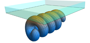
Figure 1. Diagram of a tubular body under a plane interface at  $z=0$. The distance from the place interface is denoted by $d$,
$d$,  $\boldsymbol {r}(s)$ represents the centreline of the tubular body, $\rho (s)$ is the thickness of the body at $s$,
$s$,  $\boldsymbol {\hat {t}}(s)$ is the tangent vector to the centreline and $\boldsymbol {{\hat {e}}}_{\rho }(s,\theta )$ is the local radial vector around the centreline.
This fibre parameterisation assumes that the body can be described by a single centreline,  $\boldsymbol {r}(s)$, and a continuous circular cross-sectional radius, $\rho (s)$. A different approach would be required for modelling non-traditional fibre shapes, such as a self-intersecting body or one with discontinuities in the cross-sectional radius. Furthermore, the present derivation requires that $\rho (s) \partial _s \rho (s)$ is finite everywhere to regularise the integral kernels (Koens Reference Koens2022). This differs from the standard SBT assumption that $\rho (s)$ can only vary slowly and requires ellipsoidal ends.
3. Stokes flow and the Green's function for a plane interface
The slow viscous flow around a tubular body can be accurately modelled by the incompressible Stokes equations (Kim & Karrila Reference Kim and Karrila2005)
 $$\begin{gather} \mu \nabla^2 \boldsymbol{u} - \boldsymbol{\nabla} p = \boldsymbol{0}, \end{gather}$$
 $$\begin{gather}\boldsymbol{\nabla} \boldsymbol{\cdot} \boldsymbol{u} = 0, \end{gather}$$
where  $\mu$ is the dynamic viscosity of the fluid, $\boldsymbol {u}$ is the fluid velocity and $p$ is the fluid pressure. The drag force, $\boldsymbol {F}$, and torque, $\boldsymbol {L}$, on the fluid from the tubular body are
 $$\begin{gather} \boldsymbol{F} = \iint_{S} (\boldsymbol{\sigma} \boldsymbol{\cdot} \boldsymbol{\hat{n}}_s) \,{\rm d}S, \end{gather}$$
 $$\begin{gather}\boldsymbol{L} = \iint_{S} \boldsymbol{S} \times (\boldsymbol{\sigma} \boldsymbol{\cdot} \boldsymbol{\hat{n}}_S) \,{\rm d}S, \end{gather}$$
where the integrals are taken over the surface of the body,  $\boldsymbol {\hat {n}}_S$ is the outward pointing unit normal to the surface and $\boldsymbol {\sigma } = - p \boldsymbol{\mathsf{I}} + \mu ( \boldsymbol {\nabla } \boldsymbol {u} + (\boldsymbol {\nabla }\boldsymbol {u})^{\rm T})$ is the fluid stress tensor.
The incompressible Stokes equations are linear and time independent, with the flow therefore depending only on the instantaneous geometry of the system and any boundary conditions. Hence, the drag force and torque on the fluid from rigid body motion can always be written as
 \begin{equation} \begin{pmatrix} \boldsymbol{F} \\ \boldsymbol{L} \end{pmatrix} = \boldsymbol{\mathsf{R}} \begin{pmatrix} \boldsymbol{U} \\ \boldsymbol{\varOmega} \end{pmatrix}\!, \end{equation}
where  $\boldsymbol {U}$ is the linear velocity of the body, $\boldsymbol {\varOmega }$ is the angular velocity and $\boldsymbol{\mathsf{R}}$ is the resistance matrix. The resistance matrix is often decomposed into three $3\times 3$ sub-matrices of the form
 \begin{equation} \boldsymbol{\mathsf{R}} =\begin{pmatrix} \boldsymbol{\mathsf{R}}^{FU} & \boldsymbol{\mathsf{R}}^{F\varOmega} \\ (\boldsymbol{\mathsf{R}}^{F\varOmega})^{{\rm T}} & \boldsymbol{\mathsf{R}}^{L\varOmega}, \end{pmatrix} \end{equation}
where  $\boldsymbol{\mathsf{R}}^{FU}$, $\boldsymbol{\mathsf{R}}^{F\varOmega }$ and $\boldsymbol{\mathsf{R}}^{L\varOmega }$ describe the drag force generated from translation, the drag force generated from rotation (or, equivalently, the torque generated from translation) and the torque generated from rotation, respectively.
Exact solutions of the incompressible Stokes equations, (3.1) and (3.2), only exist for simple geometries (Kim & Karrila Reference Kim and Karrila2005). As a result, most solutions are found asymptotically or numerically. Many of these asymptotic and numerical methods rely on the Green's function solution for the Stokes equations, called the Stokeslet. The Stokeslet represents the flow from a point force of strength  $\boldsymbol {f}$ on the fluid that is located at $\boldsymbol {y}$. The flow from a Stokeslet, $\boldsymbol {u}_S$, satisfies
 \begin{equation} \mu \nabla^2 \boldsymbol{u}_S - \boldsymbol{\nabla} p = \boldsymbol{f} \delta(\boldsymbol{x}-\boldsymbol{y}), \end{equation}
along with the incompressibility condition of (3.2). In free space, it is given explicitly as
 \begin{equation} 8 {\rm \pi}\mu \boldsymbol{u}_S(\boldsymbol{x}) =\boldsymbol{\mathsf{G}}_{S}(\boldsymbol{R}) \boldsymbol{\cdot} \boldsymbol{f}, \quad \boldsymbol{\mathsf{G}}_{S}(\boldsymbol{R}) = \frac{\boldsymbol{\mathsf{I}}+ \boldsymbol{{\hat{R}}}\boldsymbol{{\hat{R}}}}{|\boldsymbol{R}|}, \end{equation}
where  $\boldsymbol {x}$ is a point in the domain and we define $\boldsymbol {R}= \boldsymbol {x}-\boldsymbol {y}$ as the vector from the point force to the point of interest in the flow (Kim & Karrila Reference Kim and Karrila2005). Here, and throughout, $\boldsymbol {{\hat {R}}} = \boldsymbol {R} / \big |\boldsymbol {R}\big |$, $\hat {\cdot }$ denotes a unit-normalised vector, and $|{\cdot }|$ denotes the length of the vector.
The Stokeslet for more complicated geometries can be constructed using the representation by fundamental singularities. This method places Stokeslets and their derivatives outside the fluid region such that the boundary conditions are satisfied. Such a representation is always theoretically possible for the flow around any body (Kim & Karrila Reference Kim and Karrila2005), but the location and strengths of the singularities are often not known a priori. However, the flow due to a point force under a plane interface at  $z=0$ is known. In particular, if the fluid beneath the interface has viscosity $\mu _1$ and the fluid above the interface has viscosity $\mu _2$, the solution can be found by placing adding a Stokeslet, a force dipole (the derivative of the Stokeslet with respect to its position) and source dipole (Laplacian of the Stokeslet) in the fluid region above the interface (Aderogba & Blake Reference Aderogba and Blake1978). The resultant flow $\boldsymbol {u}_{S}^{*}$ in the lower fluid region is therefore given by
 \begin{equation} 8 {\rm \pi}\mu_{1} \boldsymbol{u}_S^{*}(\boldsymbol{x}) = \boldsymbol{\mathsf{G}}_{S}(\boldsymbol{R}) \boldsymbol{\cdot} \boldsymbol{f} + \boldsymbol{\mathsf{G}}_{S}^{*}(\boldsymbol{R}') \boldsymbol{\cdot} \boldsymbol{f}, \end{equation}
where  $\lambda = \mu _2/\mu _1$ is the viscosity ratio of the two fluids, $y_z=\boldsymbol {y} \boldsymbol {\cdot } \boldsymbol {{\hat {z}}} < 0$
 $$\begin{gather} \boldsymbol{\mathsf{G}}_{S}^{*}(\boldsymbol{R}') = \frac{\boldsymbol{\mathsf{I}}+ \boldsymbol{{\hat{R}}}' \boldsymbol{{\hat{R}}}'}{|\boldsymbol{R}'|}\boldsymbol{\cdot} \boldsymbol{\mathsf{B}} - \frac{2 \lambda}{1 + \lambda} y_z \left[(\boldsymbol{R}'\boldsymbol{\cdot}\boldsymbol{{\hat{z}}}-y_z)\frac{\boldsymbol{\mathsf{I}} - 3 \boldsymbol{{\hat{R}}}'\boldsymbol{{\hat{R}}}'}{|\boldsymbol{R}'|^3} + \frac{\boldsymbol{R}' \boldsymbol{{\hat{z}}} - \boldsymbol{{\hat{z}}} \boldsymbol{R}'}{|\boldsymbol{R}'|^3} \right]\boldsymbol{\cdot} \boldsymbol{\mathsf{A}}\,, \end{gather}$$
 $$\begin{gather}\boldsymbol{\mathsf{B}} = \frac{1 - \lambda}{1 + \lambda}\left(\boldsymbol{\mathsf{I}}- \boldsymbol{{\hat{z}}}\boldsymbol{{\hat{z}}}\right) -\boldsymbol{{\hat{z}}}\boldsymbol{{\hat{z}}}, \end{gather}$$
 $$\begin{gather}\boldsymbol{\mathsf{A}} = \boldsymbol{\mathsf{I}}- 2\boldsymbol{{\hat{z}}}\boldsymbol{{\hat{z}}}, \end{gather}$$
 $$\begin{gather}\boldsymbol{R}' = \boldsymbol{x} - \boldsymbol{\mathsf{A}} \boldsymbol{\cdot} \boldsymbol{y}, \end{gather}$$
where  $\boldsymbol {{\hat {z}}}$ is the frame vector parallel to the interface normal. In the above, $\boldsymbol{\mathsf{A}}$ is the reflection matrix across the $z=0$ plane. This solution for the flow due to a Stokeslet underneath a plane interface represents the flow under a free surface when $\lambda =0$ and a rigid wall in the limit $\lambda \to \infty$. The normal velocity of this Green's function is always 0 at the interface to keep the interface flat, while the tangential velocity at the interface is continuous and can be non-zero. As a result, the Green's function does not revert to a point force in free space when $\lambda =1$.
The Stokeslet plays an important role developing numerical and asymptotic solutions to the incompressible Stokes equations, (3.1) and (3.2). Several asymptotic theories use a representation-by-fundamental-singularities approach to construct approximate solutions for the flow around bodies with special symmetries (Keller & Rubinow Reference Keller and Rubinow1976; Johnson Reference Johnson1979). For example, some SBTs approximate the flow around an isolated slender filament by placing Stokeslets and source dipoles placed along the centreline of the fibre (Johnson Reference Johnson1979). The strength of the Stokeslets and source dipoles are determined by asymptotically expanding the no-slip boundary condition in the inverse aspect ratio of the body. This expansion sets a linear relationship between the strength of the Stokeslets and the source dipoles and relates the Stokeslet strength to the centreline velocity,  $\boldsymbol {U}_{c}(s)$, through a one-dimensional integral equation given by
 \begin{align} 8 {\rm \pi}\mu \boldsymbol{U}_{c}(s) &=\int_{-1}^{1} \left( \frac{\boldsymbol{\mathsf{I}}+ \boldsymbol{\hat{R}}_{0}\boldsymbol{\hat{R}}_{0}}{|\boldsymbol{R}_{0}|} \boldsymbol{\cdot} \boldsymbol{q}(s') -\frac{\boldsymbol{\mathsf{I}}+ \boldsymbol{\hat{t}}\boldsymbol{\hat{t}}}{|s'-s|} \boldsymbol{\cdot} \boldsymbol{q}(s) \right){\rm d}s' \nonumber\\ &\quad + \left[L_{SBT} (\boldsymbol{\mathsf{I}}+ \boldsymbol{\hat{t}}\boldsymbol{\hat{t}})+ \boldsymbol{\mathsf{I}}- 3 \boldsymbol{\hat{t}}\boldsymbol{\hat{t}} \right]\boldsymbol{\cdot}\boldsymbol{q}(s), \end{align}
where  $\boldsymbol {R}_0(s,s') = \boldsymbol {r}(s)-\boldsymbol {r}(s')$ is a vector between two points on the centreline of the body, $\boldsymbol {\hat {t}}(s) = \partial _s \boldsymbol {r}(s)$ is the tangent to the centreline, $\boldsymbol {q}(s)$ is the Stokeslet strength and $L_{SBT} =\ln [4 (1-s^{2})/(\rho ^{2}(s))]$. Although structurally similar to a one-dimensional Fredholm integral equation of the second kind, this equation does not share the same properties due to the kernel being singular, thereby making it difficult to solve (Tornberg & Shelley Reference Tornberg and Shelley2004; Tornberg Reference Tornberg2020). Even so, this formulation has been used successfully in varied circumstances (Ganguly et al. Reference Ganguly, Williams, Palacios and Goldstein2012; Qiu & Nelson Reference Qiu and Nelson2015; Lauga Reference Lauga2016; Nazockdast et al. Reference Nazockdast, Rahimian, Needleman and Shelley2017; Hernández-Pereira et al. Reference Hernández-Pereira, Guerrero, Rendón-Mancha and Tuval2019; du Roure et al. Reference du Roure, Lindner, Nazockdast and Shelley2019; Magdanz et al. Reference Magdanz2020; Li & Pumera Reference Li and Pumera2021) and derived in many different ways (Keller & Rubinow Reference Keller and Rubinow1976; Koens & Lauga Reference Koens and Lauga2018). Extensions of SBT to include boundaries tend to only apply in limited regimes (Brenner Reference Brenner1962; De Mestre & Russel Reference De Mestre and Russel1975; Jeffrey & Onishi Reference Jeffrey and Onishi1981; Barta & Liron Reference Barta and Liron1988b; Lisicki, Cichocki & Wajnryb Reference Lisicki, Cichocki and Wajnryb2016) or for a limited set of geometries (Man, Koens & Lauga Reference Man, Koens and Lauga2016; Koens & Montenegro-Johnson Reference Koens and Montenegro-Johnson2021).
Most numerical approaches to solve the incompressible Stokes equations use the Green's function nature of the Stokeslet to transform the equations into the boundary integrals (Pozrikidis Reference Pozrikidis1992; Kim & Karrila Reference Kim and Karrila2005)
 \begin{align} 4 {\rm \pi}\mu \boldsymbol{U}_{S}(\boldsymbol{x}) &= \iint_S \,{\rm d}S(\boldsymbol{x}_{0}) \left[ \boldsymbol{\mathsf{G}}(\boldsymbol{x}-\boldsymbol{x}_0) \boldsymbol{\cdot}\boldsymbol{f}(\boldsymbol{x}_{0})\right] \nonumber\\ &\quad + \mu \iint_S^{PV} \,{\rm d} S(\boldsymbol{x}_{0}) \left[\boldsymbol{U}_{S}(\boldsymbol{x}_{0})\boldsymbol{\cdot} \boldsymbol{\mathsf{T}}(\boldsymbol{x}-\boldsymbol{x}_0) \boldsymbol{\cdot} \boldsymbol{\hat{n}}_S(\boldsymbol{x}_{0}) \right], \end{align}
where all the integrals are carried out over the boundaries of the system,  $\boldsymbol {U}_{S}(\boldsymbol {x})$ is the velocity at the surface point $\boldsymbol {x}$, $\boldsymbol {\hat {n}}_S(\boldsymbol {x}_{0})$ is the surface normal pointing into the fluid, $\boldsymbol {f}(\boldsymbol {x}_{0}) = \boldsymbol {\sigma }(\boldsymbol {x}_{0}) \boldsymbol {\cdot } \boldsymbol {\hat {n}}_S(\boldsymbol {x}_{0})$ is the surface traction, $\boldsymbol{\mathsf{T}}(\boldsymbol {R})$ is the stress generated from the Stokeslet and the superscript $PV$ denotes a principal value integral. We note that the influence of background flows can be included in the boundary integral equations by replacing $\boldsymbol {U}_{S}(\boldsymbol {x})$ with $\boldsymbol {U}_{S}(\boldsymbol {x})-\boldsymbol {u}_{\infty }(\boldsymbol {x})$, where $\boldsymbol {u}_{\infty }(\boldsymbol {x})$ is the background velocity at the surface if the body was not present. The boundary integrals are exact and apply for any geometry in which the Green's function, $\boldsymbol{\mathsf{G}}$, is known (Pozrikidis Reference Pozrikidis1992). If the volume of the tubular body is constant, this equation can be transformed into the single-layer boundary integral
 \begin{equation} 8 {\rm \pi}\mu \boldsymbol{U}_{S}(\boldsymbol{x}) = \iint_S \,{\rm d} S(\boldsymbol{x}_{0}) \boldsymbol{\mathsf{G}}(\boldsymbol{x}-\boldsymbol{x}_0) \boldsymbol{\cdot}\boldsymbol{\tilde{f}}(\boldsymbol{x}_{0}), \end{equation}
where  $\boldsymbol {\tilde {f}}(\boldsymbol {x}_{0})$ represents the jump in surface traction between the exterior fluid and a fluid interior to the surface. Notably, the force and torque over any closed surface can be found identically to (3.3) and (3.4) but with $\boldsymbol {\tilde {f}}(\boldsymbol {x}_{0})$ replacing the traction (Pozrikidis Reference Pozrikidis1992).
Since the single-layer boundary integral represents the flow exactly in these circumstances (Kim & Karrila Reference Kim and Karrila2005), we can use it to develop a TBTi. Unlike other expansions of the boundary integrals (Koens & Lauga Reference Koens and Lauga2018), the TBT approach promises to create a similar one-dimensional SBT integral operator, but with a compact, symmetric and self-adjoint kernel. Furthermore the iterative solving of this operator can be used to reconstruct the jump in surface traction exactly. This overcomes several of the numerical issues encountered in SBTs and removes many of their limitations, most notably slenderness and their approximate nature. In the absence of slenderness, BEMs like that described by Pozrikidis (Reference Pozrikidis2002) are often preferred, which numerically solve the exact boundary integral equations. However, these exact methods still require the evaluation of weakly singular integrals, often via non-standard quadrature routines, and are often prohibitively expensive to apply to objects with high curvatures due to the fine surface meshes required for accuracy.
4. Tubular-body theory for interfaces
Tubular-body theory builds off key ideas from both boundary integral methods and SBTs to generate an exact theory with desirable properties. The structure of the TBT formulation is inspired by the classical SBT formalism, but overcomes several of the typical SBT restrictions to recover the exactness, flexibility and broad applicability similar to standard boundary integral approaches. To achieve this, TBT transforms the single-layer boundary integral representation into a series of well-behaved one-dimensional Fredholm integral equations of the second kind, which can be sequentially inverted to determine higher-order corrections. Fredholm integral equations of the second kind have been studied extensively and several well-established methods exist to numerically and analytically solve them (Dmitrievich & Vladimirovich Reference Dmitrievich and Vladimirovich2008). In particular, all the integral kernels within the TBT formalism are non-singular, which removes much of the complexity associated with implementing boundary integral formulations like the BEM. Though the focus of this work is on tubular bodies by plane interfaces, the development of this approach is easily generalised to other scenarios where Green's functions are available. We have presented our formulation in a manner that highlights this.
4.1. Regularisation of the boundary integrals
The single-layer boundary integral representation for a tubular body by an interface can always be expressed as
 \begin{equation} 8 {\rm \pi}\mu_1 \boldsymbol{U}_S(\boldsymbol{S}(s,\theta)) = \int\nolimits_{-1}^{1} \,{\rm d}s' \int\nolimits_{-{\rm \pi}}^{\rm \pi} \,{\rm d} \theta' \,\boldsymbol{\mathsf{G}}(s,\theta,s',\theta') \boldsymbol{\cdot} \boldsymbol{\bar{f}}(s',\theta') , \end{equation}
where  $\boldsymbol {U}_S(\boldsymbol {S}(s,\theta ))$ is the known velocity at $\boldsymbol {S}(s,\theta )$ on the surface of the body, $\boldsymbol{\mathsf{G}}(s,\theta,s',\theta ') =\boldsymbol{\mathsf{G}}_{S}(\boldsymbol {S}(s,\theta )-\boldsymbol {S}(s',\theta ')) + \boldsymbol{\mathsf{G}}_{S}^{*}(\boldsymbol {S}(s,\theta )-\boldsymbol{\mathsf{A}}\boldsymbol {\cdot }\boldsymbol {S}(s',\theta '))$ is the Green's function for the flow at $\boldsymbol {S}(s,\theta )$ from a point force located at $\boldsymbol {S}(s',\theta ')$ and $\boldsymbol {\bar {f}}(s',\theta ')$ is the unknown surface traction jump, $\boldsymbol {\tilde {f}}$, multiplied by the corresponding surface element at $(s',\theta ')$. The integrand of the boundary integrals diverges as $(s',\theta ') \to (s, \theta )$ because the free-space component of the Green's function, $\boldsymbol{\mathsf{G}}_{S}(\boldsymbol {S}(s,\theta )-\boldsymbol {S}(s',\theta '))$, blows up at this location. The interface corrections $\boldsymbol{\mathsf{G}}_{S}^{*}(\boldsymbol {S}(s,\theta )-\boldsymbol{\mathsf{A}}\boldsymbol {\cdot }\boldsymbol {S}(s',\theta '))$ are non-singular if $d>0$. The divergence of the free-space Green's function does not pose an analytical issue as the singularity is integrable over a (sufficiently smooth) surface, but it does present challenges for asymptotic and numerical approximations.
There are numerous ways to regularise boundary integral representations to overcome the singularity of the free-space kernel (Cortez, Fauci & Medovikov Reference Cortez, Fauci and Medovikov2005; Batchelor Reference Batchelor1970; Klaseboer, Sun & Chan Reference Klaseboer, Sun and Chan2012). One of the simplest is by adding and subtracting an existing solution to the boundary integral representation chosen such that the integrands cancel when  $(s',\theta ') \to (s, \theta )$. A simple solution is available for a translating spheroid in free space (Brenner Reference Brenner1963; Martin Reference Martin2019), whose translational mobility matrix $\boldsymbol{\mathsf{M}}_{A}$ and surface parameterisation $\boldsymbol {S}_{e}(s,\theta )$ we give in Appendix A. Choosing the unique spheroid that matches both the position and the tangent plane of the tubular body at $(s,\theta )$, we can add and subtract the boundary integral representation of the mobility given in (A2) from the boundary integral equations for the tubular body (4.1) to give
 \begin{align} 8 {\rm \pi}\mu_1 \boldsymbol{U}_S(\boldsymbol{S}(s,\theta)) &= \int\nolimits_{-1}^{1} \,{\rm d} s' \int\nolimits_{-{\rm \pi}}^{\rm \pi} \,{\rm d} \theta' \,\boldsymbol{\mathsf{G}}_{S}(\boldsymbol{S}(s,\theta)-\boldsymbol{S}(s',\theta')) \boldsymbol{\cdot} \boldsymbol{\bar{f}}(s',\theta')\nonumber\\ &\quad +\int\nolimits_{-1}^{1} \,{\rm d} s' \int\nolimits_{-{\rm \pi}}^{\rm \pi} \,{\rm d} \theta'\, \boldsymbol{\mathsf{G}}_{S}^{*}(\boldsymbol{S}(s,\theta)-\boldsymbol{\mathsf{A}}\boldsymbol{\cdot}\boldsymbol{S}(s',\theta')) \boldsymbol{\cdot}\boldsymbol{\bar{f}}(s',\theta')\nonumber\\ &\quad - \int\nolimits_{-1}^{1} \,{\rm d} s' \int\nolimits_{-{\rm \pi}}^{\rm \pi} \,{\rm d} \theta'\, \boldsymbol{\mathsf{G}}_{S}(\boldsymbol{S}_{e}(s_e,\theta)-\boldsymbol{S}_{e}(s',\theta')) \boldsymbol{\cdot} \boldsymbol{\bar{f}}(s,\theta) \nonumber\\ &\quad + \boldsymbol{\mathsf{M}}_{A}\boldsymbol{\cdot}\boldsymbol{\bar{f}}(s,\theta) , \end{align}
where each of  $\boldsymbol {S}_e$, $s_e$ and $\boldsymbol{\mathsf{M}}_{A}$ depend on $s$ and $\theta$. Here, and throughout, $s_e$ is the arclength on the regularising spheroid at which it intersects with the tubular body, defined in Appendix A. Notably, the matching of the tubular body and the spheroid means that the singularity in the first integrand as $(s',\theta ') \to (s,\theta )$ now precisely cancels with the singularity in the third integrand as $(s',\theta ') \to (s_e,\theta )$.
4.2. Identifying exactly integrable terms
The next step is to manipulate the regularised boundary integrals in (4.2) to find terms in the kernel that can be directly integrated. These terms and their integrals will act as the SBT-like operator in the TBT expansion, which one can think of as a first approximation to the solution. In keeping with the SBT approach, these terms should be structurally equivalent to a Fredholm integral equation of the second kind, as these are well-posed problems and have been studied extensively (Dmitrievich & Vladimirovich Reference Dmitrievich and Vladimirovich2008). This requires the expansion process to somehow allow the evaluation of the  $\theta '$ integration within (4.2) while keeping the expanded Green's function (the kernel) compact. Additionally, it will be useful if the kernel is symmetric and self-adjoint, as the operator will have real eigenvalues and additional desirable properties (Dmitrievich & Vladimirovich Reference Dmitrievich and Vladimirovich2008).
Notably, the integration over  $\theta '$ can be evaluated if all the $\theta '$ terms within the denominator of the Green's function are moved to the numerator in the expansion process (Koens & Lauga Reference Koens and Lauga2018). If done through a Taylor series of expansion in the inverse aspect ratio $\eta$, which here we do not assume is small, this recovers the classical SBT equations. The kernel of these equations is, however, not compact. Recently, there have been many attempts have been made to fix this (Walker et al. Reference Walker, Curtis, Ishimoto and Gaffney2020, Reference Walker, Ishimoto and Gaffney2023; Andersson et al. Reference Andersson, Celledoni, Ohm, Owren and Tapley2021; Tüatulea-Codrean & Lauga Reference Tüatulea-Codrean and Lauga2021; Shi, Moradi & Nazockdast Reference Shi, Moradi and Nazockdast2022; Maxian & Donev Reference Maxian and Donev2022).
In contrast to SBT, the TBT derivation creates a compact, symmetric and self-adjoint kernel by expanding each denominator in the Green's function using the binomial series. This expansion converges absolutely whenever  $(s,\theta ) \neq\ (s',\theta ')$, irrespective of the body geometry or position. In the previous TBT derivation, this was done using a single binomial expansion, motivated by an erroneous claim about the triangle inequality. Here, we correct this by applying the binomial series twice. The final structure, however, remains the same. For the full details of this manipulation, we refer the interested reader to Appendix B.
The application of sequential binomial series allows the free-space Green's function to be rewritten as
 \begin{equation} \boldsymbol{\mathsf{G}}_{S}(\boldsymbol{S}(s,\theta)-\boldsymbol{S}(s',\theta')) = \boldsymbol{\mathsf{K}}_{S}(s,s')+O( R_{\varDelta}^{(i)}(s,\theta,s',\theta')), \end{equation}
for  $i=1,2$, where $\boldsymbol{\mathsf{K}}_{S}(s,s')$ is the first-approximation kernel and equals
 \begin{equation} \boldsymbol{\mathsf{K}}_{S}(s,s') =\frac{\boldsymbol{\mathsf{I}}}{\big|\tilde{\boldsymbol{R}}\big|} + \frac{\boldsymbol{R}_0\boldsymbol{R}_0}{\big|\tilde{\boldsymbol{R}}\big|^3}. \end{equation}
Here,  $\boldsymbol {R}_0(s,s') = \boldsymbol {r}(s)-\boldsymbol {r}(s')$, $|{\tilde {\boldsymbol {R}}}|$ is a function only of $s$ and $s'$, and $R_{\varDelta }^{(i)}(s,\theta,s',\theta ')$ are remainder terms defined in Appendix B. The first approximation for the integration of the free-space Green's function therefore becomes
 \begin{align} \int\nolimits_{-1}^{1} \,{\rm d} s' \int\nolimits_{-{\rm \pi}}^{\rm \pi} \,{\rm d} \theta' \,\boldsymbol{\mathsf{G}}_{S}(\boldsymbol{S}(s,\theta)- \boldsymbol{S}(s',\theta')) \boldsymbol{\cdot} \boldsymbol{\bar{f}}(s',\theta') &\approx \int\nolimits_{-1}^{1} \,{\rm d} s' \int\nolimits_{-{\rm \pi}}^{\rm \pi} \,{\rm d} \theta' \,\boldsymbol{\mathsf{K}}_{S}(s,s') \boldsymbol{\cdot} \boldsymbol{\bar{f}}(s',\theta') \nonumber\\ &= 2 {\rm \pi}\int\nolimits_{-1}^{1} \,{\rm d} s' \,\boldsymbol{\mathsf{K}}_{S}(s,s') \boldsymbol{\cdot} \langle \,\boldsymbol{\bar{f}}(s',\theta') \rangle_{\theta'}, \end{align}
where  $\langle {\cdot } \rangle _{\theta '} = \int _{-{\rm \pi} }^{{\rm \pi} } \,{\rm d}\theta ' / (2 {\rm \pi})$. Hence, the binomial expansion has effectively treated the $\theta '$ integration and left a well-behaved integrand. This is the same kernel as found via an erroneous method in the free-space TBT formalism (Koens Reference Koens2022).
The expansion of the free-space Green's function naturally includes the regularising spheroid geometry. The result of the regularising spheroid integral can, therefore, be found by recognising that, for the spheroid,  $\boldsymbol {r}(s) \equiv a s \boldsymbol {\hat {x}}$ and $\rho (s) \equiv c \sqrt {1-s^2}$. Hence, the binomial series give
 \begin{equation} \boldsymbol{\mathsf{G}}_{S}(\boldsymbol{S}_e(s_e,\theta)-\boldsymbol{S}_e(s',\theta')) = \boldsymbol{\mathsf{K}}_{S,e}(s_e,s')+O( R_{\varDelta}^{(i)}(s_e,\theta,s',\theta')), \end{equation}
where
 $$\begin{gather} \boldsymbol{\mathsf{K}}_{S,e}(s_e,s') =\frac{\boldsymbol{\mathsf{I}}}{\big|\tilde{\boldsymbol{R}}_e\big|} + a^2(s,\theta) (s_e(s)-s')^2 \frac{\boldsymbol{\hat{t}}(s)\boldsymbol{\hat{t}}(s)}{\big|\tilde{\boldsymbol{R}}_e\big|^3} \end{gather}$$
 $$\begin{gather}\big|\tilde{\boldsymbol{R}}_e(s_e,\theta,s')\big|^2 = a^2(s,\theta)(s_e(s)-s')^2 + c^2(s) (2 - s_e^2(s) - s'^2). \end{gather}$$
The above explicitly includes the additional  $(s,\theta )$ dependence in $s_e(s)$, $a(s,\theta )$ and $c(s)$ as dictated by (A7) to (A12). The first approximation for the integration of the spheroid's Green's function therefore becomes
 \begin{align} &\int\nolimits_{-1}^{1} \,{\rm d} s' \int\nolimits_{-{\rm \pi}}^{\rm \pi} \,{\rm d} \theta' \,\boldsymbol{\mathsf{G}}_{S}(\boldsymbol{S}_e(s_e,\theta)- \boldsymbol{S}_e(s',\theta')) \boldsymbol{\cdot} \boldsymbol{\bar{f}}(s,\theta) \nonumber\\ &\quad \approx \int\nolimits_{-1}^{1} \,{\rm d} s' \int\nolimits_{-{\rm \pi}}^{\rm \pi} \,{\rm d} \theta' \,\boldsymbol{\mathsf{K}}_{S,e}(s_e(s),s') \boldsymbol{\cdot} \boldsymbol{\bar{f}}(s,\theta) \nonumber\\ &\quad = 2 {\rm \pi}\int\nolimits_{-1}^{1} \,{\rm d} s' \,\boldsymbol{\mathsf{K}}_{S,e}(s_e(s),s') \boldsymbol{\cdot} \boldsymbol{\bar{f}}(s,\theta). \end{align}
The remaining integral over  $s'$ can be evaluated exactly (Gradshteyn et al. Reference Gradshteyn, Ryzhik, Jeffrey and Zwillinger2000) to give
 \begin{equation} 2 {\rm \pi}\int\nolimits_{-1}^{1} \,{\rm d} s'\, \boldsymbol{\mathsf{K}}_{S,e}(s_e(s),s') \boldsymbol{\cdot} \boldsymbol{\bar{f}}(s,\theta) = \boldsymbol{\mathsf{M}}_{a} (s,\theta)\boldsymbol{\cdot}\boldsymbol{\bar{f}}(s,\theta), \end{equation}
where
 $$\begin{gather} \boldsymbol{\mathsf{M}}_{a} (s,\theta) = \left\{\chi_{{\parallel}}(s_e(s),\theta) \boldsymbol{{\hat{t}}}(s) \boldsymbol{{\hat{t}}}(s) +\chi_{{\perp}}(s_e(s),\theta) \left[\boldsymbol{\mathsf{I}}-\boldsymbol{{\hat{t}}}(s)\boldsymbol{{\hat{t}}}(s)\right]\right\}\!, \end{gather}$$
 $$\begin{gather}\frac{a}{2{\rm \pi}}\chi_{{\parallel}}(s_e,\theta) = \frac{1-\beta}{ (-\beta)^{3/2}}L(s_e,\theta)+g(s_e,\theta,1)-g(s_e,\theta,-1), \end{gather}$$
 $$\begin{gather}\frac{a}{2{\rm \pi}} \chi_{{\perp}}(s_e,\theta) = \frac{1}{ \sqrt{-\beta}}L(s_e,\theta), \end{gather}$$
 $$\begin{gather}L(s_e,\theta) = \ln\left(\frac{a(s_e -\beta) + \sqrt{-\beta} \big|\tilde{\boldsymbol{R}}_e(s_e,\theta,-1)\big|}{ a(s_e +\beta) + \sqrt{-\beta} \big|\tilde{\boldsymbol{R}}_e(s_e,\theta,1)\big|} \right)\!, \end{gather}$$
 $$\begin{gather}g(s_e,\theta,s') = \frac{2 (s_e-s')}{\beta \big|\tilde{\boldsymbol{R}}_e(s_e,\theta,s')\big|} \left(\frac{ s' s_e \alpha^2 - (1-s_e^2)\beta}{2\beta - s_e^2 (1-\beta) } \right)\!, \end{gather}$$
and  $a$,
$a$,  $\alpha$, $\beta$ and $s_e$ are all also functions of $(s,\theta )$ according to (A7) to (A12). The last integrand to expand contains the mirror singularities that account for the plane interface, $\boldsymbol{\mathsf{G}}_{S}^{*}(\boldsymbol {S}(s,\theta )-\boldsymbol{\mathsf{A}}\boldsymbol {\cdot }\boldsymbol {S}(s',\theta '))$. The binomial series approach can also be used to achieve this (details provided in Appendix C). The derivation shows that, for the mirror singularities, it is always possible to express the Green's function as
 \begin{equation} \boldsymbol{\mathsf{G}}_{S}^*(\boldsymbol{S}(s,\theta)-\boldsymbol{\mathsf{A}}\boldsymbol{\cdot}\boldsymbol{S}(s',\theta')) = \boldsymbol{\mathsf{K}}_{S}^*(s,s')+O( R_{\varDelta}^{*(i)}(s,\theta,s',\theta')), \end{equation}
for  $i=1,2$, where
 \begin{align} \boldsymbol{\mathsf{K}}_{S}^*(s,s')&= \left(\frac{\boldsymbol{\mathsf{I}}}{\big|\tilde{\boldsymbol{R}}^*\big|} +\frac{\boldsymbol{R}_0^* \boldsymbol{R}_0^*}{\big|\tilde{\boldsymbol{R}}^*\big|^3} \right)\boldsymbol{\cdot}\boldsymbol{\mathsf{B}} \nonumber\\ &\quad- \frac{2 \lambda}{1 + \lambda} (\boldsymbol{{\hat{z}}}\boldsymbol{\cdot}\boldsymbol{r}(s')-d) (\boldsymbol{{\hat{z}}}\boldsymbol{\cdot}\boldsymbol{r}(s)-d)\left(\frac{\boldsymbol{\mathsf{I}}}{\big|\tilde{\boldsymbol{R}}^*\big|^3} -3\frac{\boldsymbol{R}_0^* \boldsymbol{R}_0^*}{\big|\tilde{\boldsymbol{R}}^*\big|^5}\right)\boldsymbol{\cdot}\boldsymbol{\mathsf{A}}\nonumber\\ &\quad- \frac{2 \lambda}{1 + \lambda} (\boldsymbol{{\hat{z}}}\boldsymbol{\cdot}\boldsymbol{r}(s')-d) \left( \frac{\boldsymbol{R}_0^* \boldsymbol{{\hat{z}}} - \boldsymbol{{\hat{z}}} \boldsymbol{R}_0^*}{\big|\tilde{\boldsymbol{R}}^*\big|^3} \right)\boldsymbol{\cdot}\boldsymbol{\mathsf{A}}, \end{align}
where  $\boldsymbol {R}_0^*(s,s') = \boldsymbol {r}(s) - \boldsymbol{\mathsf{A}}\boldsymbol {\cdot }\boldsymbol {r}(s) -2 d \boldsymbol {{\hat {z}}}$ is a vector between a point on the body centreline and the mirror centreline, and $R_{\varDelta }^{*(i)}(s,\theta,s',\theta ')$ are the remainder terms defined in Appendix C. The first approximation for the integral of the mirror singularities is therefore
 \begin{align} &\int\nolimits_{-1}^{1} \,{\rm d} s' \int\nolimits_{-{\rm \pi}}^{\rm \pi} \,{\rm d} \theta'\, \boldsymbol{\mathsf{G}}_{S}^*(\boldsymbol{S}(s,\theta)-\boldsymbol{\mathsf{A}}\boldsymbol{\cdot}\boldsymbol{S}(s',\theta')) \boldsymbol{\cdot}\boldsymbol{\bar{f}}(s',\theta')\notag\\ &\quad \approx \int\nolimits_{-1}^{1} \,{\rm d} s' \int\nolimits_{-{\rm \pi}}^{\rm \pi} \,{\rm d} \theta'\, \boldsymbol{\mathsf{K}}_{S}^*(s,s') \boldsymbol{\cdot} \boldsymbol{\bar{f}}(s',\theta') \nonumber\\ &\quad = 2 {\rm \pi}\int\nolimits_{-1}^{1} \,{\rm d} s' \,\boldsymbol{\mathsf{K}}_{S}^*(s,s') \boldsymbol{\cdot} \langle \,\boldsymbol{\bar{f}}(s',\theta') \rangle_{\theta'}. \end{align}
The expansions of the free space (4.5), mirror (4.18) and regularising spheroid (4.10) can be combined together to create a first approximation of the regularised boundary integrals, (4.2). This approximation has the form
 \begin{equation} \mathcal{L}\bar{\boldsymbol{f}} = \Delta \boldsymbol{\mathsf{M}}_{A}(s,\theta)\boldsymbol{\cdot} \boldsymbol{\bar{f}}(s,\theta) +2 {\rm \pi}\int\nolimits_{-1}^{1} \,{\rm d} s' \left( \boldsymbol{\mathsf{K}}_{S}(s,s') +\boldsymbol{\mathsf{K}}_{S}^*(s,s')\right) \boldsymbol{\cdot} \langle \,\boldsymbol{\bar{f}}(s',\theta') \rangle_{\theta'}, \end{equation}
where  $\Delta \boldsymbol{\mathsf{M}}_{A}(s,\theta ) = \boldsymbol{\mathsf{M}}_{A}(s,\theta )- \boldsymbol{\mathsf{M}}_{a}(s,\theta )$ is the mobility for the translating spheroid, (A2), minus the first-approximation representation for this term, (4.11). Here, $\Delta \boldsymbol{\mathsf{M}}_{A}(s,\theta )$ is positive definite (see Appendix D) when $\rho (s)\neq 0$. When $\rho (s)=0$, $\Delta \boldsymbol{\mathsf{M}}_{A}(s,\theta )$ has a 0 eigenvalue in the $\boldsymbol {t} \boldsymbol {t}$ direction and so care needs to be taken to not sample the $\rho (s)=0$ points directly when numerically inverting $\mathcal {L}$. The above integral equation is the first-approximation operator that needs to be inverted for the TBT by interfaces expansion. Technically speaking, this integral equation has a compact, symmetric and self-adjoint kernel that renders the integral equation amenable to analysis and solution.
Although it involves  $(s,\theta )$, the approximate integral equation is actually a one-dimensional Fredholm integral equation of the second kind plus a sequence of linear operations (Koens Reference Koens2022). The equivalence to a one-dimensional Fredholm integral equation and a sequence of linear operations can be shown by considering the problem $\boldsymbol {Q}(s,\theta ) = \mathcal {L}\bar {\boldsymbol {f}}$. If we multiply this equation by $\Delta \boldsymbol{\mathsf{M}}_{A}^{-1}(s,\theta )$ and then average over $\theta$, it becomes
 \begin{align} \langle \Delta \boldsymbol{\mathsf{M}}_{A}^{-1}(s,\theta)\boldsymbol{\cdot} \boldsymbol{Q}\rangle_{\theta} &= \langle \,\boldsymbol{\bar{f}}(s,\theta)\rangle_{\theta}\nonumber\\ &\quad +2 {\rm \pi}\langle \Delta \boldsymbol{\mathsf{M}}_{A}^{-1}(s,\theta)\rangle_{\theta}\boldsymbol{\cdot} \int\nolimits_{-1}^{1} \,{\rm d} s' \left( \boldsymbol{\mathsf{K}}_{S}(s,s') +\boldsymbol{\mathsf{K}}_{S}^*(s,s')\right) \boldsymbol{\cdot} \langle \,\boldsymbol{\bar{f}}(s',\theta) \rangle_{\theta} , \end{align}
where we have used that  $\langle \,\boldsymbol{\bar{f}}(s',\theta ') \rangle _{\theta '} =\langle \,\boldsymbol{\bar{f}}(s',\theta ) \rangle _{\theta }$. The above is a one-dimensional Fredholm integral equation of the second kind for $\langle \,\boldsymbol{\bar{f}}(s,\theta )\rangle _{\theta }$. If this Fredholm integral equation is substituted into $\boldsymbol {Q}(s,\theta ) = \mathcal {L}\bar {\boldsymbol {f}}$, somewhat cumbersome but elementary manipulation yields
 \begin{align} \langle \Delta \boldsymbol{\mathsf{M}}_{A}^{-1}(s,\theta)\rangle_{\theta}\boldsymbol{\cdot}\Delta \boldsymbol{\mathsf{M}}_{A}(s,\theta)\boldsymbol{\cdot}\boldsymbol{\bar{f}}(s,\theta) = \boldsymbol{Q}(s,\theta) - \langle \Delta \boldsymbol{\mathsf{M}}_{A}^{-1}(s,\theta)\boldsymbol{\cdot}\boldsymbol{Q}\rangle_{\theta} + \langle \,\boldsymbol{\bar{f}}(s,\theta)\rangle_{\theta}. \end{align}
This is a linear equation for  $\boldsymbol {\bar {f}}(s,\theta )$ in terms of $\boldsymbol {Q}(s,\theta )$ and $\langle \,\boldsymbol{\bar{f}}(s,\theta )\rangle _{\theta }$. Hence, the first-approximation operator of (4.19) is equivalent to a one-dimensional Fredholm integral of the second kind with a compact, symmetric and self-adjoint kernel (4.20), plus a sequence of linear operations (4.21). Since Fredholm integral equations of the second kind and linear operations are in some sense well behaved, the inversion of the first-approximation operator, (4.19), is also expected to behave similarly.
4.3. Construct the series
The final step in the TBT derivation is to represent the full traction jump in the exact regularised boundary integrals,  $\boldsymbol {\bar {f}}(s,\theta )$, as an iterative series, found through repeatedly solving the first-approximation operator, (4.19). The simplest approach to achieve this is to add and subtract $\mathcal {L}\bar {\boldsymbol {f}}$ from the regularised boundary integrals and rearrange the equation into
 \begin{equation} 8 {\rm \pi}\boldsymbol{U}_S(\boldsymbol{S}(s,\theta)) = \mathcal{L} \bar{\boldsymbol{f}} + \Delta\mathcal{L} \bar{\boldsymbol{f}}, \end{equation}
where  $\Delta \mathcal {L} \bar {\boldsymbol {f}}$ is the difference between the first-approximation operator and right hand side of the regularised boundary integrals and is given by
 \begin{align} \Delta\mathcal{L} \bar{\boldsymbol{f}} &= \int\nolimits_{-1}^{1} \,{\rm d} s' \int\nolimits_{-{\rm \pi}}^{\rm \pi} \,{\rm d} \theta' \left[ \boldsymbol{\mathsf{G}}_{S}(\boldsymbol{S}(s,\theta)-\boldsymbol{S}(s',\theta')) - \boldsymbol{\mathsf{K}}_{S}(s,s') \right]\boldsymbol{\cdot}\boldsymbol{\bar{f}}(s',\theta') \nonumber\\ &\quad- \int\nolimits_{-1}^{1} \,{\rm d} s' \int\nolimits_{-{\rm \pi}}^{\rm \pi} \,{\rm d} \theta' \left[\boldsymbol{\mathsf{G}}_{S}(\boldsymbol{S}_{e}(s_e,\theta)-\boldsymbol{S}_{e}(s',\theta')) - \boldsymbol{\mathsf{K}}_{S,e}(s_e(s),s')\right] \boldsymbol{\cdot} \boldsymbol{\bar{f}}(s,\theta) \nonumber\\ &\quad+\int\nolimits_{-1}^{1} \,{\rm d} s' \int\nolimits_{-{\rm \pi}}^{\rm \pi} \,{\rm d} \theta' \left[\boldsymbol{\mathsf{G}}_{S}^{*}(\boldsymbol{S}(s,\theta)-\boldsymbol{\mathsf{A}}\boldsymbol{\cdot}\boldsymbol{S}(s',\theta')) - \boldsymbol{\mathsf{K}}_{S}^*(s,s') \right]\boldsymbol{\cdot}\boldsymbol{\bar{f}}(s',\theta'). \end{align}
The above expresses the difference terms as integrals to emphasise the relationship between the boundary integral and the first-approximation terms and captures all the higher-order terms from the binomial expansions.
Since the operator  $\mathcal {L}$ should be well behaved, it is reasonable to assume that its inverse exists. Assuming that an inverse $\mathcal {L}^{-1}$ exists, (4.22) can be written as
 \begin{equation} 8 {\rm \pi}\mathcal{L}^{-1}\boldsymbol{U}_S(\boldsymbol{S}(s,\theta)) = \left(1+ \mathcal{L}^{-1}\Delta\mathcal{L} \right) \bar{\boldsymbol{f}}, \end{equation}
where  $1 \bar {\boldsymbol {f}} = \bar {\boldsymbol {f}}$. The solution to the regularised boundary integrals can therefore be written as
 \begin{equation} \bar{\boldsymbol{f}}(s,\theta) = 8 {\rm \pi}\left(1+ \mathcal{L}^{-1}\Delta\mathcal{L} \right)^{-1} \mathcal{L}^{-1}\boldsymbol{U}_S(\boldsymbol{S}(s,\theta)). \end{equation}
Provided the eigenvalues of  $\mathcal {L}^{-1}\Delta \mathcal {L}$ are within $(-1,1)$, which we assume and evidence empirically later, $(1+ \mathcal {L}^{-1}\Delta \mathcal {L} )^{-1}$ can be expressed as a Neumann series, the operator analogue of a geometric series, allowing the solution to be written as
 \begin{equation} \bar{\boldsymbol{f}}(s,\theta) = 8 {\rm \pi}\sum_{n=0}^{\infty}\left(-\mathcal{L}^{-1}\Delta\mathcal{L} \right)^{n} \mathcal{L}^{-1}\boldsymbol{U}_S(\boldsymbol{S}(s,\theta)), \end{equation}
or, equivalently,
 \begin{equation} \bar{\boldsymbol{f}}(s,\theta) = \sum_{n=0}^{\infty} \bar{\boldsymbol{f}}_n(s,\theta), \end{equation}
where
 $$\begin{gather} \mathcal{L} \bar{\boldsymbol{f}}_0(s,\theta) = 8 {\rm \pi}\boldsymbol{U}(\boldsymbol{S}(s,\theta)), \end{gather}$$
 $$\begin{gather}\mathcal{L} \bar{\boldsymbol{f}}_n(s,\theta) =-\Delta\mathcal{L} \bar{\boldsymbol{f}}_{n-1}(s,\theta) \quad n\geq1. \end{gather}$$
Equations (4.27) to (4.29) are the TBTi equations for a body by a plane interface and are the main result of the paper. They are structurally equivalent to TBT for free space (Koens Reference Koens2022). Identically to the free-space version, solutions are constructed by iteratively solving a well-behaved one-dimensional Fredholm integral equation of the second kind. One-dimensional Fredholm integral equations of the second kind are well-posed structures with many established methods to solve them both numerically and analytically (Dmitrievich & Vladimirovich Reference Dmitrievich and Vladimirovich2008). In practice, the iterative approach may become efficient, depending on the difficulty of inverting the first-approximation terms and the number of terms in the series needed to achieve the desired accuracy. In the numerical implementation of TBTi described below, denoted TBT-BEM, the cost of computing additional terms in the series is exceptionally low, essentially negligible when compared with constructing discrete analogues of the linear operators (also required in the TBT-BEM approach). We note that, in the previous TBT study, no condition was identified for the convergence of the series in (4.27). The Neumann series approach used here reveals that the series converges if the eigenvalues of  $\mathcal {L}^{-1}\Delta \mathcal {L}$ are within $(-1,1)$, and applies to general operators, not simply those employed in this study.
5. Numerical implementation
One-dimensional Fredholm integral equations of the second kind can be solved in many ways (Dmitrievich & Vladimirovich Reference Dmitrievich and Vladimirovich2008). The previous TBT study inverted the first-approximation operator,  $\mathcal {L} \bar {\boldsymbol {f}}_n(s,\theta )$ in (4.28) and (4.29), and evaluated the difference integrals, $\Delta \mathcal {L} \bar {\boldsymbol {f}}_{n-1}$, through a collocation approach (Koens Reference Koens2022). This approach was simple to implement, as the kernels are all non-singular, and was effective as only a few terms in the series, (4.27), were needed. However, it would not be suitable for TBTi if significantly more terms are needed, as we will see is often the case. In light of the new conditions on $\mathcal {L}^{-1}\Delta \mathcal {L}$, we also want our method to allow us to explore the properties of our operator empirically, including estimating its spectrum. We therefore adopt a Galerkin approach (Pozrikidis Reference Pozrikidis1992; Kim & Karrila Reference Kim and Karrila2005), similar to that often applied to the boundary integral equations (Pozrikidis Reference Pozrikidis1992). We call this numerical implementation of the TBTi equations TBTi-BEM due to its similarity with traditional BEM schemes. In summary, the Galerkin method allows us to estimate the eigenvalues of the operator, quickly compute iterations and capture the full solution. As such, we have opted for versatility rather than speed in this numerical approach.
In TBTi-BEM, the surface of the tubular body is discretised by dividing  $s \in [-1,1]$ and $\theta \in [-{\rm \pi},{\rm \pi} )$ into $N$ and $M$ equal subintervals, respectively. The traction jump is then assumed to be constant over a region of $s \in [s_k-\Delta s/2,s_k+\Delta s/2]$ and $\theta \in [\theta _l- \Delta \theta /2,\theta _l+ \Delta \theta /2)$, where $(s_i,\theta _j)$ is the centre of the $(i,j)$th cell on the tubular body and $\Delta s =2/N$ and $\Delta \theta =2 {\rm \pi}/M$ are the distances between points in $s$ and $\theta$, respectively. Akin to typical boundary element methods, this discretisation approximates each surface integral as
 \begin{equation} \int\nolimits_{-1}^{1} \,{\rm d} s' \int\nolimits_{-{\rm \pi}}^{\rm \pi} \,{\rm d} \theta' \,\boldsymbol{Q}(\boldsymbol{S}(s_i,\theta_j)-\boldsymbol{S}(s',\theta')) \boldsymbol{\cdot} \boldsymbol{\bar{f}}(s',\theta') \approx \sum_{k=0}^{N} \sum_{l=0}^{M} \boldsymbol{Q}_{i,j,k,l} \boldsymbol{\cdot} \boldsymbol{\bar{f}}(s_k,\theta_l), \end{equation}
where  $\boldsymbol {Q}(\boldsymbol {R})$ represents the integral kernel of (4.19) or (4.23) and
 \begin{equation} \boldsymbol{Q}_{i,j,k,l} =\int\nolimits_{s_k-\Delta s/2}^{s_k+\Delta s/2} \,{\rm d} s' \int\nolimits_{\theta_l- \Delta \theta/2}^{\theta_l+ \Delta \theta/2} \,{\rm d} \theta'\,\boldsymbol{Q}(\boldsymbol{S}(s_i,\theta_j)-\boldsymbol{S}(s',\theta')). \end{equation}
The integrands in (4.19) and (4.23) are non-singular, by construction, and are straightforward to evaluate numerically, in contrast to those usually associated with BEMs (Pozrikidis Reference Pozrikidis2002). With the above discretisation, (4.28) and (4.29) are transformed into a system of linear equations, which can be represented as the matrix equations
 $$\begin{gather} \boldsymbol{\mathfrak{L}} \bar{\boldsymbol{\mathfrak{f}}}_0 = 8 {\rm \pi}\boldsymbol{\mathfrak{U}}, \end{gather}$$
 $$\begin{gather}\boldsymbol{\mathfrak{L}} \bar{\boldsymbol{\mathfrak{f}}}_n =- \boldsymbol{\Delta\mathfrak{L}} \bar{\boldsymbol{\mathfrak{f}}}_{n-1}, \quad n\geq1, \end{gather}$$
where  $\boldsymbol {\mathfrak {U}} = \{\boldsymbol {U}(\boldsymbol {S}(s_0,\theta _0)),\boldsymbol {U}(\boldsymbol {S}(s_1,\theta _0)), \ldots, \boldsymbol {U}(\boldsymbol {S}(s_N,\theta _M))\}$ contains the discrete surface velocities and $\bar {\boldsymbol {\mathfrak {f}}}_n = \{\bar {\boldsymbol {f}}_n(\boldsymbol {S}(s_0,\theta _0)),\bar {\boldsymbol {f}}_n(\boldsymbol {S}(s_1,\theta _0)), \ldots, \bar {\boldsymbol {f}}_n(\boldsymbol {S}(s_N,\theta _M))\}$ is the unknown traction jumps weighted by their respective surface elements. We define the discrete operators $\boldsymbol {\mathfrak {L}}$ and $\boldsymbol {\Delta \mathfrak {L}}$ as
 $$\begin{gather} \boldsymbol{\mathfrak{L}} = \begin{pmatrix} \mathfrak{L}_{0,0,0,0} & \mathfrak{L}_{0,0,1,0} & \dots & \mathfrak{L}_{0,0,N,M} \\ \mathfrak{L}_{1,0,0,0} & \mathfrak{L}_{1,0,1,0} & \dots & \mathfrak{L}_{1,0,N,M} \\ \vdots & \vdots & & \vdots\\ \mathfrak{L}_{N,M,0,0} & \mathfrak{L}_{N,M,1,0} & \dots & \mathfrak{L}_{N,M,N,M} \end{pmatrix}\!, \end{gather}$$
 $$\begin{gather}\boldsymbol{\Delta\mathfrak{L}} = \begin{pmatrix}\Delta \mathfrak{L}_{0,0,0,0} & \Delta \mathfrak{L}_{0,0,1,0} & \dots & \Delta \mathfrak{L}_{0,0,N,M} \\ \Delta \mathfrak{L}_{1,0,0,0} & \Delta \mathfrak{L}_{1,0,1,0} & \dots & \Delta\mathfrak{L}_{1,0,N,M} \\ \vdots & \vdots & & \vdots\\ \Delta \mathfrak{L}_{N,M,0,0} & \Delta \mathfrak{L}_{N,M,1,0} & \dots & \Delta \mathfrak{L}_{N,M,N,M} \end{pmatrix}\!, \end{gather}$$
as approximations to the full operators  $\mathcal {L}$ and $\Delta \mathcal {L}$, with scalar components
 \begin{gather} \mathfrak{L}_{i,j,k,l} = \int\nolimits_{s_k-\Delta s/2}^{s_k+\Delta s/2} \,{\rm d} s' \int\nolimits_{\theta_l- \Delta \theta/2}^{\theta_l+ \Delta \theta/2} \,{\rm d} \theta' \left( \boldsymbol{\mathsf{K}}_{S}(s_i,s') +\boldsymbol{\mathsf{K}}_{S}^*(s_i,s')\right) +\Delta \boldsymbol{\mathsf{M}}_{A}(s_i,\theta_j) \delta_{i,k} \delta_{j,l}, \end{gather}
 \begin{align} \Delta \mathfrak{L}_{i,j,k,l} &= \int\nolimits_{s_k-\Delta s/2}^{s_k+\Delta s/2} \,{\rm d} s' \int\nolimits_{\theta_l- \Delta \theta/2}^{\theta_l+ \Delta \theta/2} \,{\rm d} \theta' \left[ \boldsymbol{\mathsf{G}}_{S}(\boldsymbol{S}(s_i,\theta_j)-\boldsymbol{S}(s',\theta')) - \boldsymbol{\mathsf{K}}_{S}(s_i,s') \right] \nonumber\\ &\quad +\int\nolimits_{s_k-\Delta s/2}^{s_k+\Delta s/2} \,{\rm d} s' \int\nolimits_{\theta_l- \Delta \theta/2}^{\theta_l+ \Delta \theta/2} \,{\rm d} \theta' \left[\boldsymbol{\mathsf{G}}_{S}^{*}(\boldsymbol{S}(s_i,\theta_j)-\boldsymbol{\mathsf{A}}\boldsymbol{\cdot}\boldsymbol{S}(s',\theta')) - \boldsymbol{\mathsf{K}}_{S}^*(s_i,s') \right]\nonumber\\ &\quad-\delta_{i,k} \delta_{j,l} \int\nolimits_{-1}^{1} \,{\rm d} s' \int\nolimits_{-{\rm \pi}}^{\rm \pi} \,{\rm d} \theta' \left[\boldsymbol{\mathsf{G}}_{S}(\boldsymbol{S}_{e}(s_e(s_i),\theta_j)-\boldsymbol{S}_{e}(s',\theta')) -\boldsymbol{\mathsf{K}}_{S,e}(s_e(s_i),s')\right]\!. \end{align}
Here,  $\delta _{i,j}$ is the Kronecker delta, defined to be $\delta _{i,j}=1$ when $i=j$ and zero otherwise.
The discretised TBTi equations, (5.3) and (5.4), can be solved by inverting  $\boldsymbol {\mathfrak {L}}$ to find
 $$\begin{gather} \bar{\boldsymbol{\mathfrak{f}}}_0 = 8 {\rm \pi}\boldsymbol{\mathfrak{L}} ^{-1} \boldsymbol{\mathfrak{U}}, \end{gather}$$
 $$\begin{gather}\bar{\boldsymbol{\mathfrak{f}}}_n =\left(- \boldsymbol{\mathfrak{L}} ^{-1} \boldsymbol{\Delta\mathfrak{L}} \right)\bar{\boldsymbol{\mathfrak{f}}}_{n-1}, \quad n\geq1. \end{gather}$$
It is useful to retain the full  $- \boldsymbol {\mathfrak {L}} ^{-1} \boldsymbol {\Delta \mathfrak {L}}$ matrix as it reduces the task of finding higher iterations of $\bar {\boldsymbol {\mathfrak {f}}}_n$ to matrix multiplication. We note that this matrix multiplication is exceptionally fast, relative to constructing discrete analogues of the linear operators, $\boldsymbol {\mathfrak {L}}$ and $\boldsymbol {\Delta \mathfrak {L}}$.
This matrix representation also allows us to compute the infinite summation using the aforementioned Neumann series for matrices, which generalises the well-known geometric series to operators. Specifically,
 \begin{equation} \bar{\boldsymbol{\mathfrak{f}}} = \sum_{n=0}^{\infty} \bar{\boldsymbol{\mathfrak{f}}}_n = 8 {\rm \pi}\sum_{n=0}^{\infty} \left(- \boldsymbol{\mathfrak{L}} ^{-1} \boldsymbol{\Delta\mathfrak{L}} \right)^n \boldsymbol{\mathfrak{L}} ^{-1} \boldsymbol{\mathfrak{U}} = 8 {\rm \pi}(1+\boldsymbol{\mathfrak{L}} ^{-1} \boldsymbol{\Delta\mathfrak{L}} )^{-1} \boldsymbol{\mathfrak{L}} ^{-1} \boldsymbol{\mathfrak{U}}, \end{equation}
if the eigenvalues of  $\boldsymbol {\mathfrak {L}} ^{-1} \boldsymbol {\Delta \mathfrak {L}}$ lie in $(-1,1)$. These eigenvalues are an approximation to the eigenvalues of ${\mathcal {L}} ^{-1} {\Delta \mathcal {L}}$. Hence, the Galerkin approach can be used to determine the tubular-body theory by interfaces solution exactly using (5.11), estimate the eigenvalues of ${\mathcal {L}} ^{-1} {\Delta \mathcal {L}}$ and test the convergence of the series representation for the traction jump, (4.27), with relative ease.
We implemented TBTi-BEM in MATLAB® in order to validate the theory, using an optimised BEM written in Fortran 90 (Walker et al. Reference Walker, Wheeler, Ishimoto and Gaffney2019) for comparison. The time complexity of constructing the largest matrix in TBTi-BEM is  $O(N^2M^2)$, equivalent to that of a traditional BEM scheme with $NM$ elements. As expected, the optimised BEM implementation is associated with lower computational runtimes than our high-level TBTi-BEM implementation, approximately by a factor of 2–3 in typical examples. Hence, TBTi-BEM is not expected to provide any significant computational advantages over traditional BEMs, although we remark that TBTi-BEM does not require specialised quadrature schemes, whilst boundary element schemes do in general. Notably, both TBTi-BEM and BEM, which can be seen as differing formulations of the boundary integral equations, are outperformed in terms of simplicity and computational efficiency by SBTs, which are typically $O(N^2)$, although the speed of SBTs is accompanied by significantly restricted applicability and validity.
6. A spheroid by a plane wall
In order to numerically evaluate TBTi, we used TBTi-BEM to begin with perhaps the simplest class of tubular bodies: spheroids. Despite their geometrical simplicity, spheroids and the flows around them still pose challenging numerical problems in extreme circumstances, such as when very close to boundaries or when they have large aspect ratios. In this section, we explore and evidence how TBTi-BEM is capable of capturing the dynamics of such spheroids, presented with direct comparison with a numerical implementation of SBT and a BEM. We consider motion in the presence of a rigid wall, noting that motion near such a boundary generates large stresses that can be difficult to resolve numerically (Kim & Karrila Reference Kim and Karrila2005). We note that the validity of TBT has been established for non-slender and highly curved objects by Koens (Reference Koens2022), which we will see is inherited by TBTi. Hence, we will focus on evidencing validity in the presence of boundaries effects, although we will explore a more complex geometry in § 7.
Initially, we consider spheroids whose symmetry axis is taken to be parallel to the plane boundary. In such a configuration, the spheroid can be parameterised as
 \begin{equation} \boldsymbol{S}(s,\theta) = s \boldsymbol{\hat{x}} + \eta \sqrt{1-s^2} \boldsymbol{{\hat{e}}}_{\rho} -d \boldsymbol{{\hat{z}}}, \end{equation}
where we have set  $\boldsymbol {r}(s) = s \boldsymbol {\hat {x}}$ and $\rho (s) = \eta \sqrt {1-s^2}$.
6.1. Establishing accuracy with boundary element simulations
In order to verify the accuracy of TBTi-BEM (and therefore infer the versatility of the TBTi equations), we compute resistance matrices for spheroids of various aspect ratios and boundary separations. As no general analytical solutions are available for the hydrodynamic resistance of spheroids near boundaries, we compare the numerical results with those obtained with a high-accuracy BEM, as described by Walker et al. (Reference Walker, Wheeler, Ishimoto and Gaffney2019) and Pozrikidis (Reference Pozrikidis2002). Of note, as TBTi regularises the boundary integral equations by the subtraction of a free-space solution for the motion of a spheroid, not one near a boundary, accurately resolving boundary interactions remains non-trivial.
In more detail, we consider spheroids of inverse aspect ratios given by  $\eta \in \{1, 0.2, 0.1\}$ at distances $d\in \{2,2\eta, 1.1\eta \}$, encompassing both slender and non-slender objects at moderate and extreme boundary proximities. The TBTi-BEM calculations used $\lambda =10^4$, $N=15$ and $M=300$, while the boundary element calculations discretised the body into ${2\times 10^{4}}$ flat triangles. All numerical results were verified to have converged to within approximately 1 % of the values obtained using significantly higher resolution computational meshes.
In tables 1 to 3, we tabulate the absolute and relative errors in the eight non-zero resistance coefficients of the spheroids in this configuration, noting that symmetry of this particular set up removes many degrees of freedom from the resistance matrix. Here, values obtained from the boundary element simulations are considered the true values, with absolute and relative errors defined relative to these quantities. These tables, reporting the force-translation, torque-rotation and force-rotation coefficients, respectively, highlight the marked accuracy of TBTi-BEM across the range of separations and geometries considered here, particularly given the uniform, non-specific meshing employed. As might be expected, spuriously large relative errors occur for the force-rotation coefficients of table 3, which are typically  $100\times$ smaller in value than the largest coefficients, so that the observed absolute errors are in line with approximately 1 % error in computing the force density $\bar {\boldsymbol {\mathfrak {f}}}$.
Table 1. The relative error in the non-zero force-translation resistance coefficients  $\{R^{FU}_{11},R^{FU}_{22},R^{FU}_{33}\}$ for spheroids of varying aspect ratio and boundary separation, as computed with TBTi-BEM and compared against the BEM. The absolute errors between the coefficients is given in parentheses. Here, spheroids were aligned parallel to the boundary.

Table 2. The relative error in the non-zero torque-rotation resistance coefficients  $\{R^{L\varOmega }_{11},R^{L\varOmega }_{22},R^{L\varOmega }_{33}\}$ for spheroids of varying aspect ratio and boundary separation, as computed with TBTi-BEM and compared against the BEM. The absolute errors between the coefficients is given in parentheses. Here, spheroids were aligned parallel to the boundary.

Table 3. The relative error in the non-zero force-rotation resistance coefficients  $\{R^{F\varOmega }_{12},R^{F\varOmega }_{21}\}$ for spheroids of varying aspect ratio and boundary separation, as computed with TBTi-BEM and compared against the BEM. The absolute errors between the coefficients is given in parentheses. Here, spheroids were aligned parallel to the boundary.

Notably, these results suggest that TBTi is accurate even for slender objects that are very close to a boundary. In the next section, we will assess this accuracy more systematically as a function of boundary separation.
6.2. Beyond the limits of slender-body theory
While slender objects are often simulated using wall-corrected SBTs, these theories are not expected to be accurate when boundary separation is on the same scale as the radius of the object. In figure 2, we compare the effectiveness of such a numerical implementation of SBT (utilising the boundary corrections of Barta & Liron Reference Barta and Liron1988a) against TBTi-BEM by plotting computed resistance coefficients as a function of boundary separation. The TBTi equations, in principle, impose no theoretical limits on the boundary separation. Fixing  $\eta = 0.1$, figure 2 evidences the agreement between the SBT and TBTi-BEM when the boundary separation is large, here quantified by $d/\eta - 1$. However, as boundary separation decreases to approximately $\eta$ in size, the resistance coefficients computed by TBTi-BEM and SBT diverge. We also include computations using the BEM for comparison, from which we can immediately conclude that TBTi-BEM remains valid even at small separations, while the SBT is rendered inaccurate by the comparable scales of boundary separation and body radius. Hence, the validity of TBTi appears to extend significantly beyond that of this wall-corrected SBT. This reflects the fact that no slenderness assumptions are invoked in the formulation of TBTi, with the boundary integral equations being reformulated exactly.

Figure 2. The resistance coefficients for a prolate spheroid perpendicular to a wall normal as a function of gap size. (a) Force from translation along the symmetry axis of the prolate spheroid,  $R^{FU}_{11}$. (b) Force from translation along perpendicular to symmetry axis and wall normal of the prolate spheroid, $R^{FU}_{22}$. (c) Force from translation along in the direction of the wall normal, $R^{FU}_{33}$. In each plot, the TBTi-BEM result is in blue, the BEM simulations are shown are red dashed lines and the wall corrected SBT results are shown in yellow. Results are shown for $\eta =0.1$.
6.3. Replication of lubrication limits
The comparisons with the boundary element simulations and the wall corrected SBT suggests that the TBTi equations are correctly accounting for the wall at large to close distances. However, when the body gets very close to the wall, the forces on the body begin to diverge due to the lubrication stresses (Kim & Karrila Reference Kim and Karrila2005). These stresses come from the large gradients in the velocity present near the wall and are notoriously hard to resolve numerically (Ishikawa Reference Ishikawa2022). For a sphere approaching a wall the force on the fluid is known to grow as  $6 {\rm \pi}/(d-1)$, while for transverse motion the force grows proportionally to $\ln (d-1)$.
The iterative structure means the TBTi equations cannot be effectively expanded in the lubrication limit to investigate if the lubrication behaviour is preserved. It is, however, expected that the lubrication behaviour should be captured as the TBTi equations are fundamentally equivalent to the boundary integrals, which are an exact representations of the flow. We tested this by performing high resolution TBTi-BEM simulations ( $N=M=65$) for a sphere approaching a wall and compared it with the leading-order lubrication behaviour ( $6 {\rm \pi}/(d-1)$) when $d-1 \in (0.01,1]$ (figure 3). We kept the mesh uniform for all simulations. The transverse singularity requires a higher resolution and proximity to the wall than available as the gap between the sphere and wall must be minute for $\ln (d-1)$ to be large. TBTi-BEM simulations is seen to agree well with the BEM simulations for $d-1 \in (0.1,1]$ and smoothly connects to the leading-order lubrication results as $d-1<0.1$. The slight deviation between TBTi-BEM and the singularity result around $d-1= 0.01$ is due to numerical resolution issues. The TBTi-BEM is therefore able to capture the strongest lubrication singularity for a sphere, the approaching the wall singularity, suggesting that TBTi will be able to resolve the lubrication on non-spherical bodies (since TBTi is exact representation in theory).

Figure 3. The drag on a sphere as it approaches a plane wall as predicted by TBTi-BEM (blue), and the leading-order lubrication result ( $6 {\rm \pi}/(d-1)$). The BEM results for larger $d-1$ are included for reference.
6.4. Eigenvalue analysis
In order for the series defined in (4.27) to converge, and for the inverse representation of (5.11) to be valid, the eigenvalues of  $\mathcal {L}^{-1} \Delta \mathcal {L}$ are required to lie within $(-1,1)$. To establish this in practice, we consider the eigenvalues of the matrix approximation $\boldsymbol {\mathfrak {L}} ^{-1} \boldsymbol {\Delta \mathfrak {L}}$ to this operator found using TBTi-BEM. For eight of the configurations considered in § 6.1, we compute and plot the eigenvalues of this discrete operator in figure 4 in order. In each case, many of these eigenvalues can be seen to cluster above $-1$, although all remain in the required interval for convergence. Decreasing $\eta$ appears to result in the most extreme eigenvalues more closely approaching $-1$, while varying the boundary separation appears to have no noticeable effect at the scale of these plots. Hence, this suggests that the series underlying the TBTi formalism converges absolutely, an observation that appears independent of geometry, at least for the objects considered here. In a cursory evaluation of a wider range of geometries than we can succinctly report in this work, we have not encountered any objects that invalidate this observation of convergence.

Figure 4. The eigenvalues of the matrix approximation to the TBTi-BEM operator,  $\boldsymbol {\mathfrak {L}} ^{-1} \boldsymbol {\cdot } \boldsymbol {\Delta \mathfrak {L}}$, for eight of the configurations considered in § 6.1. (a) All 135 000 eigenvalues. (b) The 6000 eigenvalues closest to $-1$.
$-1$.
6.5. Convergence rates
The convergence of the TBTi summation, (5.11), as a function of the number of terms retained, was also explored for the eight different configurations in § 6.1 (figure 5) using TBTi-BEM. For brevity, only the force towards the wall from motion in the same direction,  $R^{FU}_{33}$, force in the minor axis perpendicular to the wall due to rotation around the major axis, $R^{F\varOmega }_{21}$, and the torque in the minor axis perpendicular to the wall normal from rotation in the same direction, $R^{L\varOmega }_{22}$, are shown because they converge the slowest. The force-translation and torque-rotation coefficients both correspond to motions with large lubricating stresses, while the force-rotation term is a small secondary effect of the wall.

Figure 5. The convergence of the non-zero resistance coefficients predicted by the TBTi series, (4.27) (calculated using TBTi-BEM), as a function of the truncation point in the series. The slowest coefficient to converge, in each sub-matrix, is shown for brevity. The absolute relative error is defined as the absolute value of the difference between the converged value and the iterated value all divided by the converged value. (a) The coefficient relating force towards the wall from motion towards the wall,  $R^{FU}_{33}$. (b) The coefficient relating force along the minor axis perpendicular to the wall normal from rotation around the major axis, $R^{F\varOmega }_{21}$. (c) The coefficient relating torque in the minor axis perpendicular to the wall normal from rotation in the same direction, $R^{L\varOmega }_{22}$. All coefficients are scaled by their converged value.
Except when the body is close to the wall, the coefficients are seen to converge in approximately 10 terms. A similar number of terms was needed to realise convergence in the free-space TBT equations (Koens Reference Koens2022). The number of terms needed to converge increases rapidly when the body is very close to the wall ( $d=1.1 \eta$) and as the thickness of the spheroid $\eta$ increases. The improved convergence with slender shapes is due to the first-approximation kernel capturing the local logarithmic dependence on the drag when very slender, by construction and shown in Koens (Reference Koens2022). The presence of the interface, however, introduces significant asymmetry in the traction experienced by the body and so a higher number of iterations are needed to fully resolve this variation. For the weaker lubrication singularity, present in $R^{L\varOmega }_{22}$ (figure 5c), convergence occurs around 100 terms, while for the strongest lubrication singularity, present in $R^{FU}_{33}$ (figure 5a), it takes approximately 1000 terms to converge. The small coupling term, $R^{F\varOmega }_{21}$, converges in roughly $10^{2.5} \approx 316$ terms. The singular nature of lubrication effects often makes these singularities hard to resolve numerically, so the increase in the number of terms needed for convergence is expected.
6.6. Force distribution on tilted wall-approaching spheroids
In a final example of TBTi applied to simple spheroids, we compute the force density on tilted spheroids approaching a plane wall with unit normal velocity using TBTi-BEM. In particular, we consider spheroidal geometry that is somewhat slender ( $\eta =0.1$) and at various separations, one of which lies on the edge of the regime of validity of SBT identified in § 6.2. Due to the regular integral kernel, our implementation of TBTi-BEM also does not rely on specialised quadrature routines, unlike the boundary element method used in the previous sections, so that solution via TBTi-BEM is relatively straightforward. The computed magnitude of the force on such a spheroid in three scenarios is illustrated in figure 6, from which a significant dependence on the details of the approach of the spheroid to the boundary can be seen. Here, we have made use of a fine mesh with $N=32$, $M=64$, and have considered $d\in \{0.3,0.95,1.1\}$ at angles of $\{0, {\rm \pi}/4, {\rm \pi}/2\}$ to the wall respectively. We note that he largest traction jump on the spheroid is located at the point on the surface closest to the wall, whether this is in the middle or near the ends. This is in contrast to what would be found with the wall corrected slender-body approach in which the largest stress would be found at the point on the centreline closest to the wall.

Figure 6. The computed magnitude of the force density on a range of spheroids as they approach an infinite rigid wall at unit velocity normal the boundary. Here, we have fixed  $\eta =0.1$ and considered separations of $d\in \{0.3,0.95,1.1\}$ at angles of $\{0, {\rm \pi}/4, {\rm \pi}/2\}$ to the wall in (a), (b) and (c), respectively.
7. Traction jump on helices above an interface
Tubular-body theory by interfaces applies to general cable-like bodies by any plane interface. For example, it can be used to determine the traction jump on a helix moving close to a free interface and a plane wall. We parameterise a helix by  $\rho (s) = \sqrt {1 - s^{20}}$ and $\boldsymbol {r} = r_x\boldsymbol {\hat {x}} + r_y\boldsymbol {\hat {y}} + r_z\boldsymbol {{\hat {z}}}$, where
 $$\begin{gather} r_x(s) =\alpha_h s, \end{gather}$$
 $$\begin{gather}r_y(s) = R_h\cos(ks + {\rm \pi}/2), \end{gather}$$
 $$\begin{gather}r_y(s)= R_h\sin(ks + {\rm \pi}/2), \end{gather}$$
where  $\alpha _h = \varLambda / \sqrt {{\rm \pi} ^2 R_{h}^2 + \varLambda ^2}$ is the axial length of the helix, $k ={\rm \pi} / \sqrt {{\rm \pi} ^2 R_{h}^2 + \varLambda ^2}$ is the wavenumber, $R_{h}$ is the helix radius and $\varLambda$ is the helix pitch. The helix-by-an-interface simulations here used $\eta = 0.05$, $R_h = 0.05109375$ and $\lambda = 0.25$. This parameterisation was used to simulate the motion of tightly wound helices with the free-space TBT (Koens Reference Koens2022). The specific geometry corresponds to the helix with the largest pitch and smallest helix radius tested by Koens (Reference Koens2022). When the distance from the interface was large, $d=1000$, the results found using TBTi-BEM and the free-space TBT were the same, up to numerical error.
The surface traction on this helix was determined in presence of a rigid boundary ( $\lambda \rightarrow \infty$) and a free interface ( $\lambda = 0$), using TBTi-BEM. The distance to the wall was $d = 0.15$. Each configuration is illustrated in figure 7, with figures 7(a) and 7(c) corresponding to the rigid boundary and the free interface held flat by surface tension, respectively. In both cases, we prescribe a unit velocity towards the boundary on the surface of the helix, and colour the surface by the pointwise magnitude of the resulting traction jump (multiplied by the surface element), with the boundaries shown semi-transparent for visual clarity.

Figure 7. The traction jump on a helical body as it approaches an infinite plane boundary. The colour shows the magnitude of the traction computed using TBTi-BEM for two identical helical bodies moving towards a rigid boundary (a,b) with  $\lambda \rightarrow \infty$ and a free interface (c,d) with $\lambda = 0$. In (b,d), we show the same traction distributions in the computational domain, from which we observe significant differences between different parts of each body and between the two cases. The approach towards the rigid boundary is associated with significantly larger traction, as expected.
The traction distribution on the computational domain, parameterised by arclength  $s$ and angle $\phi$, is shown in figures 7(b) and 7(d). The largest-magnitude traction jumps (multiplied by the surface element) are found on the three near-boundary regions of the helix in both cases. The decay of these peaks are skewed along the helix arms, giving the curving shape on the computational domain.
The rigid boundary is seen to generate tractions jumps (multiplied by the surface element) approximately twice as large than the free interface in these regions. Since the traction jump multiplied by the surface element scales with the total force on the body, this is consistent with the known behaviour of the lubrication force. When approaching another body, the lubrication force diverges proportionally with the inverse of the gap size,  $\Delta d$ (Kim & Karrila Reference Kim and Karrila2005). The force on the nearest points of the helix by the wall therefore scales with $1/\Delta d$. However, a helix approaching a free interface is mathematically equivalent to the helix approaching a mirrored helix across the interface. Hence, the effective gap size for the helix approaching the plane interface is doubled. The traction jump on a helix by a free interface therefore scales with $1/(2 \Delta d)$. This difference explains the apparent factor of 2 observed in the traction strengths and implies that TBTi can handle complex shapes by different types of interfaces. An investigation of the eigenvalues of the discrete TBTi-BEM operator, the convergence of the series expansion, and mesh independence can be found in Appendix E.
We further highlight the flexibility of TBTi by considering a helix that violates common assumptions of SBT, one that approaches self-intersection due to its thickness. Taking  $\eta = 0.15$ and using an increased separation $d=0.5$, we illustrate such a helix in figure 8 above a rigid boundary along with a representative computational mesh and the computed traction jump. Appendix E examines this example in more detail, including an exploration of convergence of the associated resistance matrix as a function of truncation number and mesh refinement. This non-slender, non-spheroidal example highlights the flexibility and broad utility of TBTi, even when an object is approaching self-intersection.

Figure 8. The traction field on a thick tubular body approaching a rigid boundary. (a) The geometry and magnitude of the computed surface traction jump on a helical body whose surface approaches self-intersection, where the body approaches the surface in the normal direction at unit speed. As might be expected, the largest magnitude traction jump is localised to the near-boundary side. (b) The traction jump distributions shown in the computational domain, highlighting the heterogeneous surface distribution.
8. Conclusion
This paper extends the TBT formalism to handle cable-like bodies by plane interfaces. Similarly to in the free-space case, the employed expansion allows for the traction jump on the body to be reconstructed exactly by iteratively solving a better-behaved SBT-like operator, (4.19). The iterations are shown to be equivalent to an appropriate analogue of the geometric series, indicating that the iterations will converge to the exact value if certain conditions on the eigenvalues of the operator are met. Empirically, these conditions were found to be satisfied for all geometries considered.
The TBTi equations (4.27) to (4.29) were solved numerically using a Galerkin approach (Pozrikidis Reference Pozrikidis1992) in an approach called TBTi-BEM. The Galerkin approach was taken as it provides an efficient method to conduct iterations, determine the exact solution and find approximate eigenvalues for the system, thereby empirically investigating the properties of the TBTi equations. The TBTi-BEM simulations were compared with boundary element simulations for spheroids by a plane wall. All rigid body motions near a wall generate lubrication stresses that can be hard to determine numerically. The TBTi-BEM results agreed well with both boundary element simulations for all aspect ratios and distances from the wall and the asymptotic solution to the lubrication for an approaching sphere when very close to the wall, suggesting that the TBTi equations can capture the lubrication effect. This is to be expected as TBTi is an exact representation of the flow. The largest deviations between the results were found in the weak force-rotation resistance coefficients and was likely due to the numerical errors in both the TBTi-BEM and BEM implementations.
The TBTi equations were found to converge in around 10 iterations when the body was well separated from the boundary, based on the results of TBTi-BEM. However, when very close to the wall, the rate of convergence decreased. When a body approaches the plane wall it was found to converge in around 1000 terms, while for other motions it took around 100 terms. The increase in the number of terms reflects the general difficulty with resolving lubrication effects numerically.
Finally, the TBTi simulations (TBTi-BEM) were used to look at the motion of helices towards a rigid wall and a free interface. As would be anticipated, the traction (multiplied by the surface element) found in both cases was largest on the parts of the helix closest to the interface and decayed as the distance increased. The maximum traction on the helix near a plane wall was also found to be around twice the size of the maximum traction on the helix by a free interface. Since the hydrodynamics of a body by a free interface is equivalent to two bodies approaching each other at double the separation, the factor of two is consistent with the scaling of the lubrication singularity.
The TBTi formalism opens up many new possibilities for exploration. It allows a SBT-like method to explore geometries that lie well beyond the limits of SBT in the presence of interfaces. Further, it presents a viable alternative to general boundary integral methods, removing the need to evaluate weakly singular integrals during numerical solution. Looking forward, we expect that the convergence rate of the representation can be improved should a better regularising body be found, which is a topic of active development for TBT and TBTi. The derivation could also generalise to other systems that can be represented by integral equations, and other viscous flow configurations. Furthermore, the well-behaved nature of the TBTi operator opens up new avenues for solving for the hydrodynamics of wires near interfaces asymptotically.
Funding
B.J.W. is supported by the Royal Commission for the Exhibition of 1851. The TBTi-BEM program and data that support the findings of this study are openly available on GitHub at https://github.com/LKoens/TBTi.
Declaration of interests
The authors report no conflict of interest.
Appendix A. Spheroid solution and matching
We make use of the exact solution for the mobility of a translating spheroid in order to regularise the boundary integral equations of our tubular body. We parameterise the surface of a spheroid as
 \begin{equation} \boldsymbol{S}_{e}(s,\theta) = a s \boldsymbol{\hat{x}}' + c \sqrt{1-s^2} \boldsymbol{\hat{\rho}}(\theta) +\boldsymbol{q}, \end{equation}
where  $a$ and $c$ are the semi-axes of the spheroid, $\boldsymbol {\hat {x}}'$ is a unit vector along the symmetry axis, $\boldsymbol {\hat {\rho }}(\theta )$ is the radial director perpendicular to the symmetry axis and $\boldsymbol {q}$ is the centre of the spheroid. The solution of Brenner (Reference Brenner1963) gives
 \begin{equation} \boldsymbol{\mathsf{M}}_{A}\boldsymbol{\cdot}\boldsymbol{\bar{f}}(s,\theta) = \int\nolimits_{-1}^{1} \,{\rm d} s' \int\nolimits_{-{\rm \pi}}^{\rm \pi} \,{\rm d} \theta'\, \boldsymbol{\mathsf{G}}_{S}(\boldsymbol{S}_{e}(s,\theta)-\boldsymbol{S}_{e}(s',\theta')) \boldsymbol{\cdot} \boldsymbol{\bar{f}}(s,\theta) , \end{equation}
where  $\alpha = c/a$ is the inverse aspect ratio of the spheroid. The matrix $\boldsymbol{\mathsf{M}}_A$ is proportional to the translational mobility matrix of the spheroid and equals
 $$\begin{gather} \boldsymbol{\mathsf{M}}_{A} = \zeta_{{\parallel}} \boldsymbol{\hat{x}}' \boldsymbol{\hat{x}}' + \zeta_{{\perp}} (\boldsymbol{\mathsf{I}} -\boldsymbol{\hat{x}}' \boldsymbol{\hat{x}}'), \end{gather}$$
 $$\begin{gather}\frac{a \beta^{3/2}}{4 {\rm \pi}\mu_1} \zeta_{{\parallel}} = (\beta-1) \arccos(\alpha^{-1}) + \sqrt{\beta}, \end{gather}$$
 $$\begin{gather}\frac{a \beta^{3/2}}{2 {\rm \pi}\mu_1} \zeta_{{\perp}} = (3\beta+1) \arccos(\alpha^{-1}) - \sqrt{\beta}, \end{gather}$$
 $$\begin{gather}\beta = \alpha^2-1. \end{gather}$$
 In regularising the boundary integral equations for the tubular body (4.1), we fit a spheroid to the surface of the tubular body at a point  $(s,\theta )$ by matching the positions and the tangent planes of the two objects. Since the spheroid parameterisation has four independent parameters ( $a, \boldsymbol {\hat {x}}', c, \boldsymbol {q}$), it is possible to enforce these conditions uniquely, with the point of agreement on the regularising spheroid parameterised as $(s_e,\theta )$, where $s_e$ is the arclength of the spheroid at which the surface and tangent plane matches. Explicitly, we require $\boldsymbol {S}_e(s_e,\theta ) = \boldsymbol {S}(s,\theta )$, $\partial _{s_e}\boldsymbol {S}_e(s_e,\theta ) =\partial _{s} \boldsymbol {S}(s,\theta )$ and $\partial _{\theta }\boldsymbol {S}_e(s_e,\theta ) =\partial _{\theta } \boldsymbol {S}(s,\theta )$. These conditions give the following relationships between the surface of the body and the parameterisation of the spheroid:
 $$\begin{gather} \boldsymbol{\hat{x}}' = \boldsymbol{\hat{t}}(s), \end{gather}$$
 $$\begin{gather}\boldsymbol{\hat{\rho}}(\theta) = \boldsymbol{{\hat{e}}}_{\rho}(s,\theta), \end{gather}$$
 $$\begin{gather}\boldsymbol{q} +a s_e \boldsymbol{\hat{x}}'= \boldsymbol{r}(s), \end{gather}$$
 $$\begin{gather}2 c^2 = \rho^2(s) + \rho(s) \sqrt{\rho^2(s)+4(\partial_s \rho(s))^2}, \end{gather}$$
 $$\begin{gather}a = 1 - \boldsymbol{\hat{t}}(s) \boldsymbol{\cdot} \partial_s \boldsymbol{{\hat{e}}}_{\rho}(s,\theta), \end{gather}$$
 $$\begin{gather}c^2 s_e = \rho(s) \partial_s \rho(s), \end{gather}$$
where  $\boldsymbol {\hat {t}}(s) = \partial _{s} \boldsymbol {r}(s)$ is the tangent to the centreline of the body.
Appendix B. Expanding the free-space boundary integral kernel
In order to cast the boundary integrals in the TBT form, first, one writes the argument of the free-space Green's function as
 \begin{equation} \boldsymbol{S}(s,\theta)-\boldsymbol{S}(s',\theta') = \boldsymbol{R}_0(s,s') + \Delta \boldsymbol{{\hat{e}}}_{\rho}(s,\theta,s',\theta') , \end{equation}
where  $\boldsymbol {R}_0(s,s') = \boldsymbol {r}(s)-\boldsymbol {r}(s')$ is a vector between two points on the centreline of the body and $\Delta \boldsymbol {{\hat {e}}}_{\rho }(s,\theta,s',\theta ') = \rho (s) \boldsymbol {{\hat {e}}}_{\rho }(s,\theta ) -\rho (s') \boldsymbol {{\hat {e}}}_{\rho }(s',\theta ')$ is the difference between the cross-section vectors at $(s,\theta )$ and $(s',\theta ')$. The length squared of the argument is therefore
 \begin{align} \big|\boldsymbol{S}(s,\theta)-\boldsymbol{S}(s',\theta')\big|^2 = \big|\boldsymbol{R}_0(s,s')\big|^2 + \big|\Delta \boldsymbol{{\hat{e}}}_{\rho}(s,\theta,s',\theta')\big|^2 + 2 \boldsymbol{R}_0(s,s') \boldsymbol{\cdot} \Delta \boldsymbol{{\hat{e}}}_{\rho}(s,\theta,s',\theta'), \end{align}
where the first two terms are the squared lengths of each of the vectors in (B1) while the last term is the cross-term. This equation can be rewritten as
 \begin{align} \big|\boldsymbol{S}(s,\theta)-\boldsymbol{S}(s',\theta')\big|^2 = \left[\big|\boldsymbol{R}_0(s,s')\big|^2 + \big|\Delta \boldsymbol{{\hat{e}}}_{\rho}(s,\theta,s',\theta')\big|^2 \right]\left[1+ R_{\varDelta }^{(1)}(s,\theta,s',\theta')\right], \end{align}
where
 \begin{align} \left[\big|\boldsymbol{R}_0(s,s')\big|^2 + \big|\Delta \boldsymbol{{\hat{e}}}_{\rho}(s,\theta,s',\theta')\big|^2 \right] R_{\varDelta }^{(1)}(s,\theta,s',\theta') = 2 \boldsymbol{R}_0(s,s') \boldsymbol{\cdot}\Delta \boldsymbol{{\hat{e}}}_{\rho}(s,\theta,s',\theta'). \end{align}
The size of  $R_{\varDelta }^{(1)}(s,\theta,s',\theta ')$ can be bound with the triangle inequality. The triangle inequality implies that for any two vectors $\boldsymbol {a}$ and $\boldsymbol {b}$, $|{\boldsymbol {a}}|^2 + |{\boldsymbol {b}}|^2 \geq 2 |{\boldsymbol {a} \boldsymbol {\cdot } \boldsymbol {b}}|$, with equality holding if and only if $\boldsymbol {a}=\pm \boldsymbol {b}$. If $\boldsymbol {a} = \boldsymbol {R}_0(s,s')$ and $\boldsymbol {b} = \Delta \boldsymbol {{\hat {e}}}_{\rho }(s,\theta,s',\theta ')$, $\boldsymbol {a}=\pm \boldsymbol {b}$ can only occur if the tubular body intersects itself. Hence, provided that the body does not self-intersect, the triangle inequality shows that $|{R_{\varDelta }^{(1)}(s,\theta,s',\theta ')}| < 1$ for all $(s',\theta ')$. This same bound does not hold when considering the cross-terms that result from a sum of three vectors, rather than two. This was the erroneous assumption that led to the error in the original TBT derivation, although this does not impact on the derived formalism.
The bound on  $R_{\varDelta }^{(1)}(s,\theta,s',\theta ')$ prompts the denominator of each of the terms within the free-space Green's function to be written as
 \begin{align} &\big|\boldsymbol{S}(s,\theta)-\boldsymbol{S}(s',\theta')\big|^{-2n}\nonumber\\ &\quad = \left[\big|\boldsymbol{R}_0(s,s')\big|^2 + \big|\Delta \boldsymbol{{\hat{e}}}_{\rho}(s,\theta,s',\theta')\big|^2\right]^{-n} \left[1+ R_{\varDelta}^{(1)}(s,\theta,s',\theta')\right]^{-n}, \end{align}
which is structurally equivalent to a binomial series. Generally, a binomial series can be written as
 \begin{equation} (1+x)^\varsigma =
\sum_{k=0}^{\infty}\begin{pmatrix}{\varsigma}\\
{k}\end{pmatrix}x^k,
\end{equation}
\begin{equation} (1+x)^\varsigma =
\sum_{k=0}^{\infty}\begin{pmatrix}{\varsigma}\\
{k}\end{pmatrix}x^k,
\end{equation}where the generalised binomial coefficient is given by
 \begin{equation} \begin{pmatrix}{\varsigma}\\ {k} \end{pmatrix} = \frac{1}{k!} \prod_{n=0}^{k+1} (\varsigma-n). \end{equation}
The binomial series converges absolutely if  $|{x}|<1$ and $\varsigma \in \mathbb {C}$. Therefore, taking $\varsigma =-n$ and $x = R_{\varDelta }^{(1)}(s,\theta,s',\theta ')$, the denominators in the free-space Green's function can be expressed as
 \begin{align} &|\boldsymbol{S}(s,\theta)-\boldsymbol{S}(s',\theta')|^{-2n} \nonumber\\ &\quad = \left[\big|\boldsymbol{R}_0(s,s')\big|^2 + \big|\Delta \boldsymbol{{\hat{e}}}_{\rho}(s,\theta,s',\theta')\big|^2\right]^{-n} \sum_{k_1=0}^{\infty}\begin{pmatrix}{-n}\\ {k_1} \end{pmatrix} R_{\varDelta}^{(1)}(s,\theta,s',\theta')^{k_1}. \end{align}
This first binomial series moves the  $\theta '$ that is related to the dot product of $\boldsymbol {R}_0(s,s')$ and $\Delta \boldsymbol {{\hat {e}}}_{\rho }(s,\theta,s',\theta ')$ from the denominator to the numerator of the Green's function. However, $\theta '$ dependence remains within the $|{\Delta \boldsymbol {{\hat {e}}}_{\rho }(s,\theta,s',\theta ')}|^2$ term of the denominator.
The  $\theta '$ dependence that remains within the denominator can be addressed with a second binomial series. Similarly to the first expansion, the length squared of $\Delta \boldsymbol {{\hat {e}}}_{\rho }(s,\theta,s',\theta ')$ can be written as
 \begin{equation} \big|\Delta \boldsymbol{{\hat{e}}}_{\rho}(s,\theta,s',\theta')\big|^2 = \rho^2(s) +\rho^2(s') - 2 \rho(s) \rho(s') \boldsymbol{{\hat{e}}}_{\rho}(s,\theta) \boldsymbol{\cdot} \boldsymbol{{\hat{e}}}_{\rho}(s',\theta'), \end{equation}
allowing the remaining terms in the denominator to be expressed as
 \begin{equation} \big|\boldsymbol{R}_0(s,s')\big|^2 + \big|\Delta \boldsymbol{{\hat{e}}}_{\rho}(s,\theta,s',\theta')\big|^2 = \big|\tilde{\boldsymbol{R}}(s,s')\big|^2 \left[1+ R_{\varDelta}^{(2)}(s,\theta,s',\theta')\right]\!, \end{equation}
where
 $$\begin{gather} \big|\tilde{\boldsymbol{R}}(s,s')\big|^2 = \big|\boldsymbol{R}_0(s,s')\big|^2 + \rho^2(s) + \rho^2(s'), \end{gather}$$
 $$\begin{gather}\big|\tilde{\boldsymbol{R}}(s,s')\big|^2 R_{\varDelta}^{(2)}(s,\theta,s',\theta') =- 2 \rho(s) \rho(s') \boldsymbol{{\hat{e}}}_{\rho}(s,\theta) \boldsymbol{\cdot} \boldsymbol{{\hat{e}}}_{\rho}(s',\theta'). \end{gather}$$
Similarly to the first expansion, the triangle inequality tells us that  $\rho ^2(s) + \rho ^2(s') \geq 2 \rho (s) \rho (s') |{ \boldsymbol {{\hat {e}}}_{\rho }(s,\theta ) \boldsymbol {\cdot } \boldsymbol {{\hat {e}}}_{\rho }(s',\theta ')}|$. This means that $|{R_{\varDelta }^{(2)}(s,\theta,s',\theta ')}|< 1$ for $s \neq s'$ because the distance between any two points on the centreline is greater than zero, $|{\boldsymbol {R}_0(s,s')} |>0$, when $s \neq s'$. If $s=s'$, the distance between points on the centreline goes to zero, so that $|{\boldsymbol {R}_0(s,s')}| =0$ and the triangle inequality becomes $1 \geq |{\boldsymbol {{\hat {e}}}_{\rho }(s,\theta ) \boldsymbol {\cdot } \boldsymbol {{\hat {e}}}_{\rho }(s,\theta ')}|$. Hence, $|{R_{\varDelta }^{(2)}(s,\theta,s,\theta ')}|=1$ if the local radial vector at $(s,\theta )$, $\boldsymbol {{\hat {e}}}_{\rho }(s,\theta )$, is parallel to the vector at $(s,\theta ')$, $\boldsymbol {{\hat {e}}}_{\rho }(s,\theta ')$. These local radial vectors are parallel if $\theta =\theta '+m {\rm \pi}$, where $m$ is an integer, meaning that $|{R_{\varDelta }^{(2)}(s,\theta,s',\theta ')}|<1$ if $(s,\theta ) \neq\ (s', \theta '+m{\rm \pi} )$. A binomial series in $R_{\varDelta }^{(2)}(s,\theta,s',\theta ')$, therefore, allows us to express the denominators as
 \begin{align} &|\boldsymbol{S}(s,\theta)-\boldsymbol{S}(s',\theta')|^{-2n} \nonumber\\ &\quad = |\tilde{\boldsymbol{R}}(s,s')|^{-2n} \sum_{k_1=0}^{\infty} \begin{pmatrix}{-n}\\ {k_1}\end{pmatrix} R_{\varDelta}^{(1)}(s,\theta,s',\theta')^{k_1} \sum_{k_2=0}^{\infty} \begin{pmatrix}{-n}\\ {k_2}\end{pmatrix} R_{\varDelta}^{(2)}(s,\theta,s',\theta')^{k_2}, \end{align}
if  $(s,\theta ) \neq\ (s',\theta '+m {\rm \pi})$. Geometrically, $|\tilde {\boldsymbol {R}}(s,s')|^2$ is the total squared lengths of $\boldsymbol {R}_0(s,s')$, $\rho (s)\boldsymbol {\hat {e}}_\rho (s,\theta )$ and $\rho (s')\boldsymbol {\hat {e}}_\rho (s',\theta ')$, while the $R_{\varDelta }^{(i)}(s,\theta,s',\theta ')$ contain the interactions between the vectors, where $i=1,2$.
The summation over  $k_2$ does not converge when $(s,\theta ) = (s',\theta '+m {\rm \pi})$. However, these points are treated with the regularisation of the boundary integrals. The spheroid used in the regularised boundary integrals, (4.2), was chosen to mimic the dimensions and tangent plane of the tubular body at $(s,\theta )$. This means that the radius and radial directors $\boldsymbol {{\hat {e}}}_{\rho }$ of the spheroid match with the body at this location. Hence, when $s=s'$, the terms $|{\tilde {\boldsymbol {R}}}|$, $R_{\varDelta }^{(1)}(s,\theta,s,\theta ')$ and $R_{\varDelta }^{(2)}(s,\theta,s,\theta ')$ are the same form for the tubular body and the regularising spheroid. The subtraction of the spheroid geometry in the regularised boundary integrals, (4.2), causes each term of the binomial expanded free-space kernel for the tubular body to cancel with its counterpart from the regularising spheroid, removing the convergence issue when $(s,\theta ) = (s',\theta '+m {\rm \pi})$. This is by construction.
Appendix C. Expanding the mirror boundary integral kernel
Similarly to the free-space Green's function expansion, the expansion of the image kernels starts by expressing the argument as
 \begin{equation} \boldsymbol{S}(s,\theta)-\boldsymbol{\mathsf{A}}\boldsymbol{\cdot}\boldsymbol{S}(s',\theta') = \boldsymbol{R}_0^*(s,s') + \Delta\boldsymbol{{\hat{e}}}_{\rho}^*(s,\theta,s',\theta') , \end{equation}
where  $\boldsymbol {R}_0^*(s,s') = \boldsymbol {r}(s) - \boldsymbol{\mathsf{A}}\boldsymbol {\cdot }\boldsymbol {r}(s) -2 d \boldsymbol {{\hat {z}}}$ is a vector between a point on the body centreline and the mirror centreline, $\Delta \boldsymbol {{\hat {e}}}_{\rho }^*(s,\theta,s',\theta ') =\rho (s) \boldsymbol {{\hat {e}}}_{\rho }(s,\theta ) - \rho (s') \boldsymbol{\mathsf{A}}\boldsymbol {\cdot }\boldsymbol {{\hat {e}}}_{\rho }(s',\theta ')$ is the difference between the cross-section vectors at $(s,\theta )$ and the mirror cross-section vector at $(s',\theta ')$ and $\boldsymbol{\mathsf{A}}$ is the reflection matrix in $\boldsymbol {{\hat {z}}}$. The length squared of the argument can therefore be expressed as
 \begin{align} \big|\boldsymbol{S}(s,\theta)-\boldsymbol{\mathsf{A}} \boldsymbol{\cdot}\boldsymbol{S}(s',\theta')\big|^2 = \big|\tilde{\boldsymbol{R}}^*(s,s')\big|^2 \left[1+ R_{\varDelta}^{*(2)}(s,\theta,s',\theta')\right]\left[1+ R_{\varDelta}^{*(1)}(s,\theta,s',\theta')\right], \end{align}
where
 $$\begin{gather} \big|\tilde{\boldsymbol{R}}^*(s,s')\big|^2 = \boldsymbol{R}_0^{*2}(s,s') + \rho^2(s) + \rho^2(s'), \end{gather}$$
 $$\begin{gather}\big|\tilde{\boldsymbol{R}}^*(s,s') \big|^2R_{\varDelta}^{*(2)}(s,\theta,s',\theta') =- 2 \rho(s) \rho(s') \boldsymbol{{\hat{e}}}_{\rho}(s,\theta) \boldsymbol{\cdot} \boldsymbol{\mathsf{A}}\boldsymbol{\cdot}\boldsymbol{{\hat{e}}}_{\rho}(s',\theta'), \end{gather}$$
 $$\begin{gather}\big|\tilde{\boldsymbol{R}}^*(s,s')\big|^2 \left[1+ R_{\varDelta}^{*(2)}(s,\theta,s',\theta')\right]R_{\varDelta}^{*(1)}(s,\theta,s',\theta') = 2 \boldsymbol{R}_0^*(s,s') \boldsymbol{\cdot}\Delta\boldsymbol{{\hat{e}}}_{\rho}^*(s,\theta,s',\theta'). \end{gather}$$
Geometrically,  $|\tilde {\boldsymbol {R}}^*(s,s')|^2$ is again the total squared lengths of each component vector in (C1), while the $R_{\varDelta }^{*(i)}(s,\theta,s',\theta ')$ contains the interactions between them. Unlike the free-space case, $R_{\varDelta }^{*(2)}(s,\theta,s',\theta ')<1$ for all $(s',\theta ')$ because $|{\boldsymbol {R}_0^*(s,s')}| \neq 0$ if the body does not cross the interface. The binomial series, which follow, are therefore always valid. Hence, the denominators in our mirror Green's functions can always be expanded as
 \begin{align}
&\big|\boldsymbol{S}(s,\theta)-\boldsymbol{\mathsf{A}}\boldsymbol{\cdot}\boldsymbol{S}(s',\theta')\big|^{-2n}
\nonumber\\ &\quad
=\big|\tilde{\boldsymbol{R}}^*(s,s')\big|^{-2n}
\sum_{k_1=0}^{\infty} \left(\begin{smallmatrix}{-n}\\
{k_1}\end{smallmatrix}\right)R_{\varDelta}^{*(1)}(s,\theta,s',\theta')^{k_1}
\sum_{k_2=0}^{\infty}\left(\begin{smallmatrix}{-n}\\ {k_2}\end{smallmatrix}\right)R_{\varDelta}^{*(2)}(s,\theta,s',\theta')^{k_2}.
\end{align}
\begin{align}
&\big|\boldsymbol{S}(s,\theta)-\boldsymbol{\mathsf{A}}\boldsymbol{\cdot}\boldsymbol{S}(s',\theta')\big|^{-2n}
\nonumber\\ &\quad
=\big|\tilde{\boldsymbol{R}}^*(s,s')\big|^{-2n}
\sum_{k_1=0}^{\infty} \left(\begin{smallmatrix}{-n}\\
{k_1}\end{smallmatrix}\right)R_{\varDelta}^{*(1)}(s,\theta,s',\theta')^{k_1}
\sum_{k_2=0}^{\infty}\left(\begin{smallmatrix}{-n}\\ {k_2}\end{smallmatrix}\right)R_{\varDelta}^{*(2)}(s,\theta,s',\theta')^{k_2}.
\end{align}Appendix D. Properties of  $\Delta \boldsymbol{\mathsf{M}}_{A}(s,\theta )$

The matrix  $\Delta \boldsymbol{\mathsf{M}}_{A}(s,\theta ) = \boldsymbol{\mathsf{M}}_{A} - \boldsymbol{\mathsf{M}}_a$ represents the difference between the exact solution for the effective ellipsoid and the first-approximation term and is important to for invertibility properties of the $\mathcal {L}$ operator. For example, (4.21) shows that $\boldsymbol {\bar {f}}(s,\theta )$ is linearly related to the driving flow $\theta$ dependence through $\Delta \boldsymbol{\mathsf{M}}_{A}(s,\theta )^{-1}$. We therefore require $\Delta \boldsymbol{\mathsf{M}}_{A}(s,\theta )$ to be invertible for all $s$ and $\theta$. This can be shown by considering the integrals of the remaining terms.
By definition,  $\Delta \boldsymbol{\mathsf{M}}_{A}(s,\theta )$ is a diagonal matrix with at most two distinct eigenvalues, corresponding to eigenvectors that are parallel and perpendicular to $\boldsymbol {t} \boldsymbol {t}$, which follows directly from the structures of $\boldsymbol{\mathsf{M}}_{A}$ and $\boldsymbol{\mathsf{M}}_a$. Explicitly, we can write
 \begin{equation} \Delta \boldsymbol{\mathsf{M}}_{A} = \lambda_1 \boldsymbol{t} \boldsymbol{t} + \lambda_2 (\boldsymbol{\mathsf{I}}- \boldsymbol{t} \boldsymbol{t}), \end{equation}
where  $\lambda _1= \zeta _{\parallel } - \chi _{\parallel }$ and $\lambda _2 =\zeta _{\parallel } - \chi _{\parallel }$. The inverse of $\Delta \boldsymbol{\mathsf{M}}_{A}(s,\theta )$ can therefore be found by taking the reciprocal of these eigenvalues provided they are not 0.
From the boundary integral representation, these eigenvalues can be written as
 \begin{align} \lambda_1 &= \int_{-1}^{1}\,{\rm d}s'\int_{-{\rm \pi}}^{\rm \pi}\,{\rm d}\theta'\, \boldsymbol{t}\boldsymbol{\cdot}\left[\boldsymbol{\mathsf{G}}_{S}(\boldsymbol{S}_e(s_e,\theta)-\boldsymbol{S}_e(s',\theta')) -\boldsymbol{\mathsf{K}}_{S,e}(s_e(s),s')\right]\boldsymbol{\cdot}\boldsymbol{t} \nonumber\\ &= I_1 + I_2 \end{align}
 \begin{align} \lambda_2 &= \int_{-1}^{1}\,{\rm d}s'\int_{-{\rm \pi}}^{\rm \pi}\,{\rm d}\theta'\, \boldsymbol{b} \boldsymbol{\cdot}\left[\boldsymbol{\mathsf{G}}_{S}(\boldsymbol{S}_e(s_e,\theta)-\boldsymbol{S}_e(s',\theta')) - \boldsymbol{\mathsf{K}}_{S,e}(s_e(s),s')\right]\boldsymbol{\cdot} \boldsymbol{b} \nonumber\\ &= I_1 + I_3 , \end{align}
where  $\boldsymbol {b} \boldsymbol {\cdot } \boldsymbol {t} =0$ and we define
 $$\begin{gather} I_1 = \int_{-1}^{1}\,{\rm d}s'\int_{-{\rm \pi}}^{\rm \pi}\,{\rm d}\theta' \left[\frac{1}{|\boldsymbol{R}_{e}|} -\frac{1}{| \tilde{\boldsymbol{R}}_{e}|} \right]\!, \end{gather}$$
 $$\begin{gather}I_2 = \int_{-1}^{1}\,{\rm d}s'\int_{-{\rm \pi}}^{\rm \pi}\,{\rm d}\theta' \left[\frac{a^2(s)(s-s')^2}{|\boldsymbol{R}_{e}|^3} -\frac{a^2(s)(s-s')^2}{| \tilde{\boldsymbol{R}}_{e}|^3} \right]\!, \end{gather}$$
 $$\begin{gather}I_3 = \int_{-1}^{1}\,{\rm d}s'\int_{-{\rm \pi}}^{\rm \pi}\,{\rm d}\theta' \frac{(\boldsymbol{b}\boldsymbol{\cdot}\Delta \boldsymbol{{\hat{e}}}_{\rho})^2}{|\boldsymbol{R}_{e}|^3}. \end{gather}$$
Inspection reveals that the integrand of  $I_3$ is non-negative, so that positivity of $\lambda _2$ relies only on the positivity of $I_1$. The behaviours of $I_1$ and $I_2$ are less clear. However, progress can be made by recognising that the negative terms in the integrands of $I_1$ and $I_2$ are simply the first terms in the binomial expansions of the remaining integrands, found in Appendix B. Hence, $I_1$ and $I_2$ can be written in terms of the tails of the binomial series
 $$\begin{gather} I_1 = \int_{-1}^{1}\,{\rm d}s' \frac{1}{| \tilde{\boldsymbol{R}}_{e}|} \int_{-{\rm \pi}}^{\rm \pi}\,{\rm d}\theta' \sum_{k_2=1}^{\infty} \left(\begin{smallmatrix}{-1/2}\\ {k_2}\end{smallmatrix}\right) \left[-\varrho \cos(\theta-\theta') \right]^{k_2}, \end{gather}$$
 $$\begin{gather}I_2 = \int_{-1}^{1}\,{\rm d}s' \frac{a^2(s)(s-s')^2}{| \tilde{\boldsymbol{R}}_{e}|^3} \int_{-{\rm \pi}}^{\rm \pi}\,{\rm d}\theta' \sum_{k_2=1}^{\infty} \left(\begin{smallmatrix}{-3/2}\\ {k_2}\end{smallmatrix}\right) \left[- \varrho \cos(\theta-\theta') \right]^{k_2}, \end{gather}$$
where  $\varrho = 2 \rho (s) \rho (s') /| \tilde {\boldsymbol {R}}_{e}|^2$ and we have used that $R^{(1)}_{\varDelta } = 0$ for the spheroid geometry. Interchanging the summation and integration and evaluating the $\theta '$ integral gives
 $$\begin{gather} I_1 = \int_{-1}^{1}\,{\rm d}s' \frac{1}{| \tilde{\boldsymbol{R}}_{e}|} \sum_{k_2=1}^{\infty} \left(\begin{smallmatrix}{-1/2}\\ {2 k_2}\end{smallmatrix}\right) \varrho^{2 k_2} \frac{2 \sqrt{\rm \pi} \varGamma(k_2 + 1/2)}{k_2!}, \end{gather}$$
 $$\begin{gather}I_2 = \int_{-1}^{1}\,{\rm d}s' \frac{a^2(s)(s-s')^2}{| \tilde{\boldsymbol{R}}_{e}|^3} \sum_{k_2=1}^{\infty} \left(\begin{smallmatrix}{-3/2}\\ {2 k_2}\end{smallmatrix}\right) \varrho^{2 k_2} \frac{2 \sqrt{\rm \pi} \varGamma(k_2 + 1/2)}{k_2!}. \end{gather}$$
These summations can be evaluated exactly to give
 $$\begin{gather} I_1 = \int_{-1}^{1}\,{\rm d}s' \frac{1}{| \tilde{\boldsymbol{R}}_{e}|} \left[ \frac{4 K\left(2 \varrho/(1+\varrho) \right)}{ \sqrt{1+\varrho}} - 2 {\rm \pi}\right]\!, \end{gather}$$
 $$\begin{gather}I_2 = 2 {\rm \pi}\int_{-1}^{1}\,{\rm d}s' \frac{a^2(s)(s-s')^2}{| \tilde{\boldsymbol{R}}_{e}|^3} \left[ _2F_1 \left(\frac{3}{4},\frac{5}{4}; 1; \varrho^2 \right)-1 \right]\!, \end{gather}$$
where  $K(x)$ is the complete elliptic integral of the first kind and $_2F_1(a,b;c;x)$ is Gauss's hypergeometric function. The above integrands are strictly greater than zero unless $\varrho =0$ for all $s'$. Since $\varrho =0$ for all $s'$ can only occur if $\rho (s)=0$, this implies that $I_1>0$ and $I_2>0$ unless $\rho (s)=0$, at which point $I_1=I_2=0$. Therefore, we have that
 $$\begin{gather} \lambda_1 = I_1 + I_2 > 0 \end{gather}$$
 $$\begin{gather}\lambda_2 = I_1 + I_3 > 0 \end{gather}$$
unless  $\rho (s)=0$. Hence, $\Delta \boldsymbol{\mathsf{M}}_{A}(s,\theta )$ is invertible provided $\rho (s) \neq 0$, which typically holds at all points except the endpoints of a tubular body.
Appendix E. Eigenvalues and convergence for a thick helix
In order to further explore the example of § 7 in which a tubular body approaches self-intersection, we investigate the convergence of the resistance matrix as a function of the number of terms taken in (4.27) and the level of mesh refinement, report in figures 9(a) and 10, respectively. From these explorations, we see that TBTi-BEM converges rapidly with mesh refinement and with truncation number, with the latter expectedly being the slower of the two. In particular, the relatively small change (<1 %) in accuracy observed for meshes with  $N=M\gtrapprox 30$ justifies the use of what otherwise might be thought of as coarse meshes when using TBTi-BEM.

Figure 9. Convergence as a function of truncation number and an eigenvalue analysis. (a) For the thicker helix of § 7, illustrated in figure 8, we assess the convergence of the resistance matrix as a function of the number of terms taken in the series of (4.27). Error is measured in the Frobenius norm relative to the result corresponding to 1001 terms. Rates of convergence are in line with those associated with spheroids at similar boundary separations (see § 6). (b) For the same helix, we plot the eigenvalues of the discrete operator, which are all seen to lie strictly within  $(-1,1)$. Here, the tubular body is discretised with $N=M=60$ and we have taken $d=0.5$.

Figure 10. The convergence of resistance matrices as a function of mesh resolution. For the slender helix of § 7, we compute the relative error in the TBTi-BEM resistance matrices as a function of mesh refinement, varying  $N=M$ for a fixed configuration. The error is computed as the Frobenius norm of the difference between the result at a given mesh resolution and that obtained with $N=M=160$, and appears to decrease approximately with $N^3=M^3$. The relative error falls below 1 % by $N=M=20$ in this case.
Additionally, figure 9(b) reports the distribution of eigenvalues of the discrete operator  $\mathfrak {L}^{-1}\Delta \mathfrak {L}$, from which it is evident that the eigenvalues of the discrete operator lie in $(-1,1)$. Hence, the discretised series representation of the TBTi formalism (TBTi-BEM) is convergent, as supported by the direct assessment of convergence in figure 9(a). By comparison with § 6 and the convergence analysis presented there for spheroids, this example suggests that the convergence of TBTi is not materially impaired by the complex geometry considered here.
Separately, in order to verify the approximate mesh independence of the TBTi-BEM calculations, we investigate the convergence of the resistance matrix as a function of mesh resolution. Taking  $N=M$ and considering the slender helix of § 7, the relative error in the resistance matrix is plotted in figure 10. Here, we are evaluating the error via the Frobenius norm relative to the result of taking a very fine mesh with $N=M=160$. The computed resistance matrix can be seen to converge rapidly as the mesh is refined, with the error displaying an approximately cubic dependence on the mesh resolution. Here, we have taken 1001 terms in the series of (4.27).


