


Introduction
The Greenland ice sheet (GrIS) is the second largest land ice mass on Earth and one of the largest contributors to global sea-level rise (Rignot and others, Reference Rignot, Velicogna, Van Den Broeke, Monaghan and Lenaerts2011; Gardner and others, Reference Gardner2013; Khan and others, Reference Khan2014). Observations indicate that its contribution increased from 0.09 mm a−1 for the period 1992–2001 to 0.68 mm a−1 for 2012–2016 (IPCC, Reference Pörtner, Roberts, Masson-Delmotte, Zhai, Tignor, Poloczanska, Mintenbeck, Nicolai, Okem, Petzold, Rama and Weyer2019, Section 4.2.2). Apart from a negative surface mass balance due to melting, this contribution to sea level rise is driven by speed-up and retreat of marine-terminating glaciers, leading to ice thinning (Howat and others, Reference Howat, Joughin and Scambos2007; Rignot and others, Reference Rignot, Velicogna, Van Den Broeke, Monaghan and Lenaerts2011; Gillet-Chaulet and others, Reference Gillet-Chaulet2012; IPCC, Reference Pörtner, Roberts, Masson-Delmotte, Zhai, Tignor, Poloczanska, Mintenbeck, Nicolai, Okem, Petzold, Rama and Weyer2019). Of particular importance for sea-level predictions are observations of ice streams that transport ice from the interior of the ice sheet to the margin, where it either melts or calves into icebergs. Dynamic processes of ice sheets in Greenland and Antarctica have been progressively included in numerical models to project sea-level changes (Robinson and others, Reference Robinson, Calov and Ganopolski2012; Church and others, Reference Church2013; Goelzer and others, Reference Goelzer2020; Rückamp and others, Reference Rückamp, Goelzer and Humbert2020). To simulate present ice stream flow and determine its contribution to the mass balance of ice sheets, we have to understand the natural variability of ice stream dynamics on time scales of tens to thousands of years (Robel and others, Reference Robel, Degiuli, Schoof and Tziperman2013). For an accurate assessment of the dynamic component of mass loss, ice-sheet flow requires high-resolution observations of the kinematic properties and the geometry conditions.
Ice stream characteristics vary in their geographical settings and thus boundary conditions, for instance ice thickness, subglacial topography, resistive properties of the underlying substrate, subglacial hydrology, as well as atmospheric and oceanic forcing (Robel and others, Reference Robel, Degiuli, Schoof and Tziperman2013; Khan and others, Reference Khan2014b; Aschwanden and others, Reference Aschwanden, Fahnestock and Truffer2016). In contrast to flow of outlet glaciers, which often drain ice through bedrock channels or valleys, the high flow velocities of ice streams extend further into the interior of the ice sheet. In some cases their location is not controlled by the bed topography and their boundaries are characterized by narrow shear zones (Truffer and Echelmeyer, Reference Truffer and Echelmeyer2003). Basal properties of ice streams in Greenland have been mostly investigated at the (now sub-marine) ice-sheet margins of paleo glacier beds with multi-beam bathymetry and marine sediment cores (e.g. Dowdeswell and others, Reference Dowdeswell2014; Hogan and others, Reference Hogan, Ó Cofaigh, Jennings, Dowdeswell and Hiemstra2016; Newton and others, Reference Newton2017). The beds of paleo ice streams can be hard or soft and often show a large number of streamlined bedforms, mostly parallel to ice flow (Roberts and others, Reference Roberts, Long, Davies, Simpson and Schnabel2010). Streamlined bedforms underneath contemporary ice streams in Antarctica have been analyzed by King and others (Reference King, Hindmarsh and Stokes2009) and Bingham and others (Reference Bingham2017) and classified as mega-scale glacial lineations (MSGL) (Stokes and Clark, Reference Stokes and Clark2002). As subglacial structures may have formed over multiple glaciations, their interpretation is often challenging (Roberts and Long, Reference Roberts and Long2005). Little is known about the current conditions of ice stream beds in the central regions of the GrIS, at the onset of streaming ice flow, because data acquisition as well as determination of the geometry and composition of the bed is much more difficult to elaborate than on the continental shelf. For central Greenland it was generally assumed until recently that the ice sheet is underlain by lithified sediment or a crystalline basement. However, a detailed study of Christianson and others (Reference Christianson2014) identifies deformable and water saturated sediment several meters thick at the onset zone of the Northeast Greenland Ice Stream (NEGIS), which indicates that deformation of the basal substrate could influence sliding at the ice–bed interface and probably also limit subglacial erosion. Furthermore, Jezek and others (Reference Jezek2011) detect elongated landforms probably formed by erosion at the base of the southern flank of the Jakobshavn Ice Stream. Both interpretations indicate a more complex interplay of basal conditions and ice dynamics than present in the case of a simply hard-based ice sheet in Greenland's interior.
The NEGIS is one of the most prominent features of the GrIS. With a length of ~ 600 km it drains ~12% of the GrIS via fast-flowing marine-terminating glaciers (Rignot and Mouginot, Reference Rignot and Mouginot2012). Surface ice flow velocities vary from 10 m a−1 at the onset to more than 2000 m a−1 at the grounding line of the outlet glaciers (Mouginot and others, Reference Mouginot, Rignot, Scheuchl and Millan2017). The NEGIS differs from all other marine-terminating glaciers in Greenland with its catchment of fast streaming ice flow almost reaching the central ice divide (Joughin and others, Reference Joughin, Smith and Howat2018). This configuration provides a possible mechanism to transmit forcing from the marine area far inland (Christianson and others, Reference Christianson2014) and several studies have assessed potential changes in the stability of the NEGIS and the ice dynamics in Northeast Greenland (Fahnestock and others, Reference Fahnestock, Abdalati, Joughin, Brozena and Gogineni2001; Joughin and others, Reference Joughin, Smith, Howat, Scambos and Moon2010; Bamber and others, Reference Bamber2013; Khan and others, Reference Khan2014).
To fully understand the dominating processes and basal boundary conditions driving NEGIS ice flow, in particular in its onset region, on-site measurements are most useful. So far, geophysical surveys investigating the upstream part of the NEGIS concentrated on the immediate surroundings of the East Greenland Ice-core Project (EGRIP) drill site (Fig. 1b), where the ice stream widens (Keisling and others, Reference Keisling2014; Vallelonga and others, Reference Vallelonga2014). High basal melt rates caused by higher continental geothermal heat flux close to the ice divide, as a remnant of the passing of the Icelandic hot spot, are assumed to cause the onset of the ice stream (Fahnestock and others, Reference Fahnestock, Abdalati, Joughin, Brozena and Gogineni2001; Rogozhina and others, Reference Rogozhina2016; Martos and others, Reference Martos2018). Further downstream, acceleration is likely caused by subglacial water routing and the presence of high porosity, water-saturated deformable subglacial till, which lubricates the ice stream (Christianson and others, Reference Christianson2014). The geophysical data of Christianson and others (Reference Christianson2014) suggest that subglacial till is distributed in the center of our survey region, across the entire ice stream, and is dilatant in the fast-flowing part of the ice stream. The source and routing of till is not yet fully understood. The presence of unconsolidated sediment inside and outside of the NEGIS suggest that sediments are funneled into the NEGIS from the upstream catchment (Christianson and others, Reference Christianson2014). Overall, it is difficult to assess which processes dominate the different regions of the ice stream and how they interact (Schlegel and others, Reference Schlegel, Larour, Seroussi, Morlighem and Box2015).
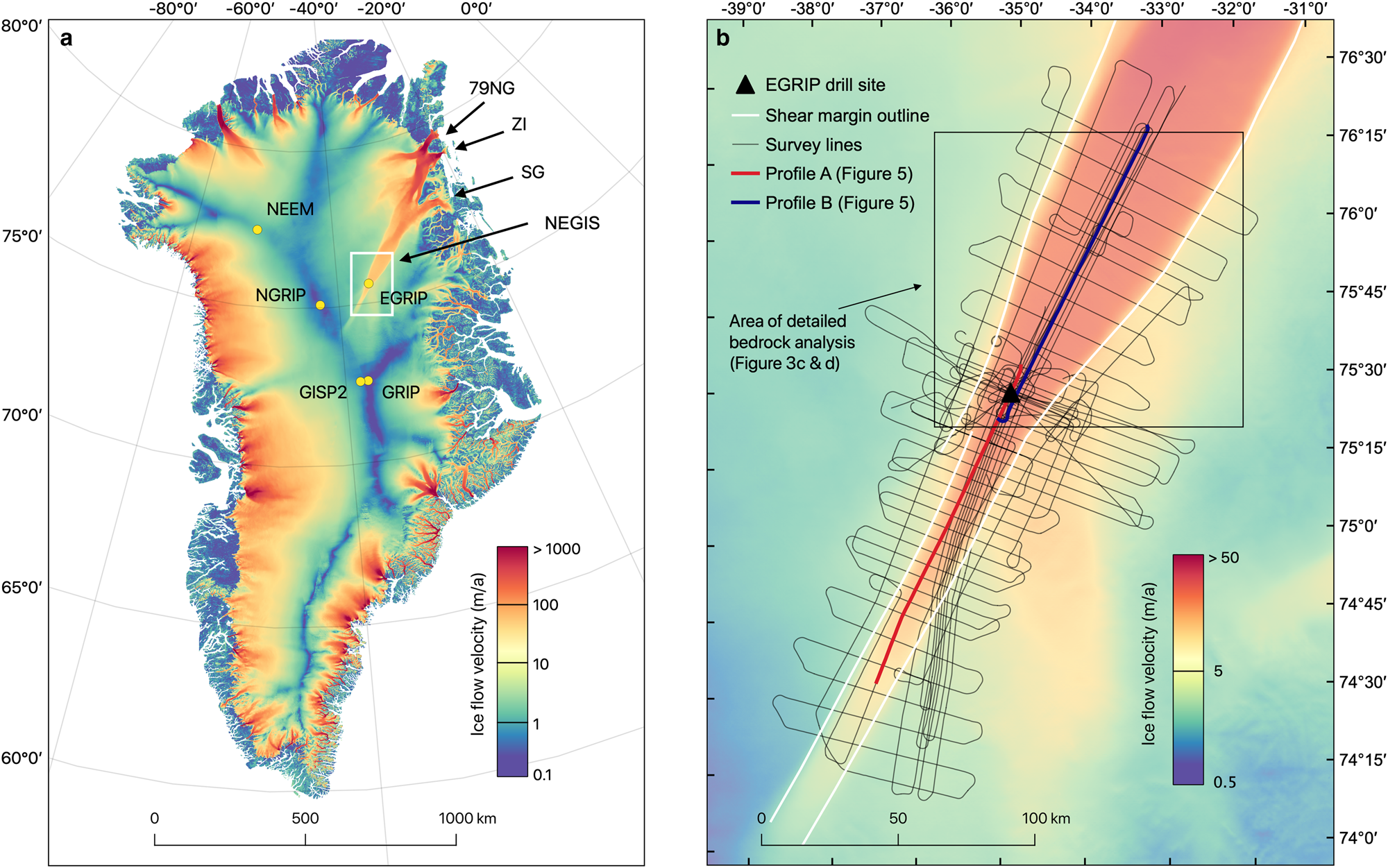
Fig. 1. (a) Surface velocity map of the Greenland ice sheet, highlighting the NEGIS and its marine-terminating outlets (79NG, Zachariae Isbrae (ZI) and Storstrømmen Glacier (SG)). The survey area (b) is marked with a white outline. (b) Ice flow velocity field of the survey area. The schematic outline of the shear margin was derived from Landsat images. Both maps are displayed in WGS 84/NSIDC Sea Ice Polar Stereographic North (EPSG:3413) and show velocity data of Joughin and others (Reference Joughin, Smith and Howat2018).
The most important factors controlling ice streams are their basal properties, ice thickness and bed topography, especially as studies of subglacial hydrology are dependent upon bed and surface slope and thus the variation in ice thickness on a local to regional scale (Wright and others, Reference Wright, Siegert, Le Brocq and Gore2008). Without a sufficient spatial data coverage also at the onset of ice streams, it is not possible to assess the nature of the ice stream bed and its properties. Over the last five decades, most radio-echo sounding campaigns have concentrated on ice divides, domes or fast-flowing outlet glaciers (Bamber and others, Reference Bamber2013; Fretwell and others, Reference Fretwell2013). To date, several bed elevation models for Greenland exist (e.g. Bamber and others, Reference Bamber2013; Morlighem and others, Reference Morlighem2017) with variable resolution and data coverage. Furthermore, modeling studies reveal that an interpretation of isochrones of ice streams is challenging without a detailed knowledge of the bed topography (Leysinger Vieli and others, Reference Leysinger Vieli, Hindmarsh and Siegert2007). These existing limitations motivated the acquisition of new high-resolution ice thickness data to improve available bed topographies around NEGIS, in order to help interpret basal structures and thereby determine ice–substrate interaction within NEGIS and in its vicinity (Keisling and others, Reference Keisling2014; Vallelonga and others, Reference Vallelonga2014).
In this paper, we use airborne radio-echo sounding data to extend previous geophysical surveys of ice thickness and internal layering around the EGRIP drill site. We provide a new high-resolution bed topography map and discuss the overall glaciological setting in the context of NEGIS’ ice dynamics. Furthermore, we interpret radar returns from subglacial structures, which are not visible in our bed topography DEM, to deduce bed properties and complement simple interpretations based on ice thickness only.
Data and Methods
Survey area
The radar data were recorded in the vicinity of the EGRIP drill site in May 2018. A total area of ~24 000 km2 was mapped with 8233 km of profiles sub-parallel and perpendicular to the ice flow direction (Fig. 1b). The central part of the survey area, in direct vicinity to the EGRIP drill site, was covered with a profile spacing of 5 km, further up- and downstream the spacing is 10 km. The area reaches from 150 km upstream to 150 km downstream of the EGRIP drilling site and covers, both, shear margins and parts of the slow-flowing areas outside and adjacent to the ice stream. The shear margins, as boundaries of the ice stream, are mapped over a distance of more than 250 km. The survey lines also cover the transition zone of two northwestern shear margins, located southwest of the EGRIP drill site. Several profiles follow flow paths of a point on the ice surface that has passed through the shear margin.
Radar system
Since 2016 the Alfred Wegener Institute, Helmholtz Centre for Polar and Marine Research (AWI) has been operating a multi-channel ultra-wideband (UWB) airborne radar sounder and imager for sounding ice thickness and imaging internal layering and the basal interface of polar ice sheets. The Multichannel Coherent Radar Depth Sounder (MCoRDS) was developed at the Center for Remote Sensing of Ice Sheets (CReSIS) at the University of Kansas in 1993 and has been continuously improved (Gogineni and others, Reference Gogineni2001; Shi and others, Reference Shi2010). This radar system is designed to operate with multiple antenna elements to increase the power radiated to the target and to compensate for unwanted signals from side echoes and surface clutter by multi-looking and steering a beam to a desired orientation. A comprehensive description of AWI's UWB radar system is given by Hale and others (Reference Hale2016), Rodriguez-Morales and others (Reference Rodriguez-Morales2014) and Wang and others (Reference Wang2014). Its full capabilities were demonstrated by Kjær and others (Reference Kjær2018). The radar system is installed on the fuselage of the AWI Polar6 Basler BT-67 aircraft and comprises eight transmit channels to transmit and receive radar signals, with a high power transmit and receiver module with fast switching speed. All antenna elements were oriented in along-track (HH) polarization. The radar system is able to alternate between different pulse duration stages and different receiver gains for each stage to increase the dynamic range. GPS data were acquired by four geodetic NovAtel DL-V3 GNSS receivers operating at 20 Hz. After processing we achieve a positioning accuracy of 3–4 cm in horizontal space and 10 cm in elevation for the aircraft.
Data acquisition
Signals were transferred in three stages with different pulse durations and gains (see Table I). The transmitted waveforms are amplitude-tapered with a Tukey window with a taper ratio of 0.08 to reduce range sidelobes caused by the sudden transitions of the envelope in a standard chirped pulse without losing much transmit power (Li and others, Reference Li2013). To reduce the data rate and writing speed and to increase signal to noise ratio (SNR), coherent integrations (presums) with zero-pi modulation (Allen and others, Reference Allen, Mozaffar and Akins2005) are performed for each waveform depending on the acquisition mode. The aircraft altitude on all survey flights was ~365 m above ground level and the data were acquired at a pulse repetition frequency of 10 kHz. With an aircraft speed of ~260 km h−1 this results in an initial horizontal transmitting interval of about 0.7 cm. All profiles were recorded in our narrow band (NB) mode with a frequency range of 180–210 MHz.
Table 1. Acquisition parameters of AWI's UWB radar campaign in Greenland 2018
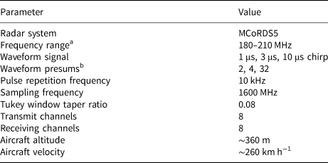
aFrequency range from 180 to 210 MHz is referred to narrow band mode (NB).
bPresums are set for each waveform individually.
Data processing
For data processing, we use the CReSIS Toolbox algorithms for all three spatial domains: vertical range (pulse compression), along-track (fk migration) and cross track (array processing) (see CReSIS-Toolbox, 2019). Further detailed description of the radar data processing is given in the Appendix.
Surface and bed detection
Radar data are recorded in the time domain in two-way travel time (TWT). To convert from radar time to depth, we use the same relative dielectric constant of 3.15 for depth-conversion as used for synthetic aperture radar (SAR) processing. No compensation was done for a firn layer because the spatial variability of firn properties in dynamic regimes can vary on a scale of a few kilometers (Dutrieux and others, Reference Dutrieux2013). The detection of the ice surface is performed automatically by applying a threshold filter searching for the first maximum in a given time window. This window depends on the flight altitude of the aircraft over ground. The location of the surface reflection has been verified using the seismic processing and interpretation software Paradigm by Emerson E&P.
At several locations, the range detection of the bed reflector was not clear. Off-nadir reflections offered multiple horizons for bed picks in regions with rough bed topography, where scattered off-nadir reflections and the nadir bed are simultaneously present. In most cases, we selected the strongest reflection, because the nadir return signal is usually stronger than off-nadir scattered signals. However, this was not always the case, especially in the areas of strong internal deformation, where englacial layers of high reflectivity reduce the energy and mask the bed return.
Nested bed topography model
We computed an ice thickness and bed elevation model based on our observed ice thickness. We integrate them into the existing dataset of Morlighem and others (Reference Morlighem2017), BedMachine v3 (BMv3), in order to get a better overview of the regional topographic setting. We create a buffer of 5 km around our flight lines, use our ice thickness inside this buffer and BMv3 data outside of it. To prevent a strong gradient at the edges of the buffer, we apply a block mean filter on our output grid. The ice thickness data are subtracted from the DEM of the Greenland Ice Mapping Project (GIMP) ice surface (Howat and others, Reference Howat, Negrete and Smith2014). This particular DEM was used in order to compare our bed topography with the BMv3 bed, which also uses GIMP as a reference surface. The grid has been created with the adjustable tension continuous curvature splines method. We also use a tension factor of 0.5 to suppress undesired oscillations and a convergence factor of 0.15% of our gradient in input data. The output grid has a cell size of 500 m and elevations are referenced to mean sea-level using the geoid EIGEN-6C4 (Förste and others, Reference Förste2014). For all bed elevation maps we used the Polar Stereographic North (70 °N, 45 °W) projection, which corresponds to ESPG 3413.
Uncertainty analysis
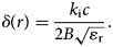
We take the root mean square (RMS) error of the range resolution and add the RMS error of the dielectric constant (CReSIS-Toolbox, 2019). This analysis requires an exact detection of the ice surface, which is well constrained for our data. To determine range resolution variability, we performed a crossover analysis of bed picks at 1449 profile intersections and calculated the mean deviation h c. For the dielectric constant, we consider an error on the order of 1% for typical dry ice (Bohleber and others, Reference Bohleber, Wagner and Eisen2012) and obtain for the range uncertainty:
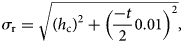
with the radar wave two-way travel time t and a mean value for crossover deviation, h c, of 8.03 m. For ice thickness ranging from 2000 to 3000 m our error, σr, ranges from 13 to 17 m.
Results
Ice thickness and bed topography model
The mean ice thickness of our survey area is 2748 m and varies from 2059 m (±13 m) to 3092 m (±17 m). We observe a gradual decrease of ice thickness from the onset of the NEGIS close to the ice divide toward northeast (Fig. 2). Upstream of the EGRIP drill site we observe an increase in the spatial variability of ice thickness. The variation in ice thickness is mainly dominated by basal topography because the ice surface shows only small changes in surface deviation and slope. We present our bed elevation model (EGRIP-NOR-18) as a nested bed elevation model in Figure 3. The data agree overall with recent Greenland bed topography models of Bamber and others (Reference Bamber2013) and Morlighem and others (Reference Morlighem2017). Bed elevation in our study region ranges from −293 m (±17 m) to 606 m (±13 m). The area of lowest bed elevation in our survey region is located southwest of the EGRIP drill site. Bed topography is generally lower and shows less spatial variability upstream of EGRIP. The topography downstream shows higher mean elevation and also more variability of a few hundred meters elevation change over a distance of 5–10 km.
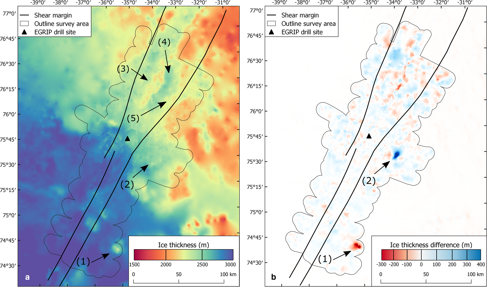
Fig. 2. (a) Map of ice thickness distribution based on the data of the AWI radar survey 2018, termed EGRIP-NOR-2018. EGRIP-NOR-2018 ice thickness minus BMv3 ice thickness is shown in the right image (b). Blue colors represent higher and red colors lower ice thickness in our dataset, respectively. The numbers 1–5 indicate the locations of the main features.
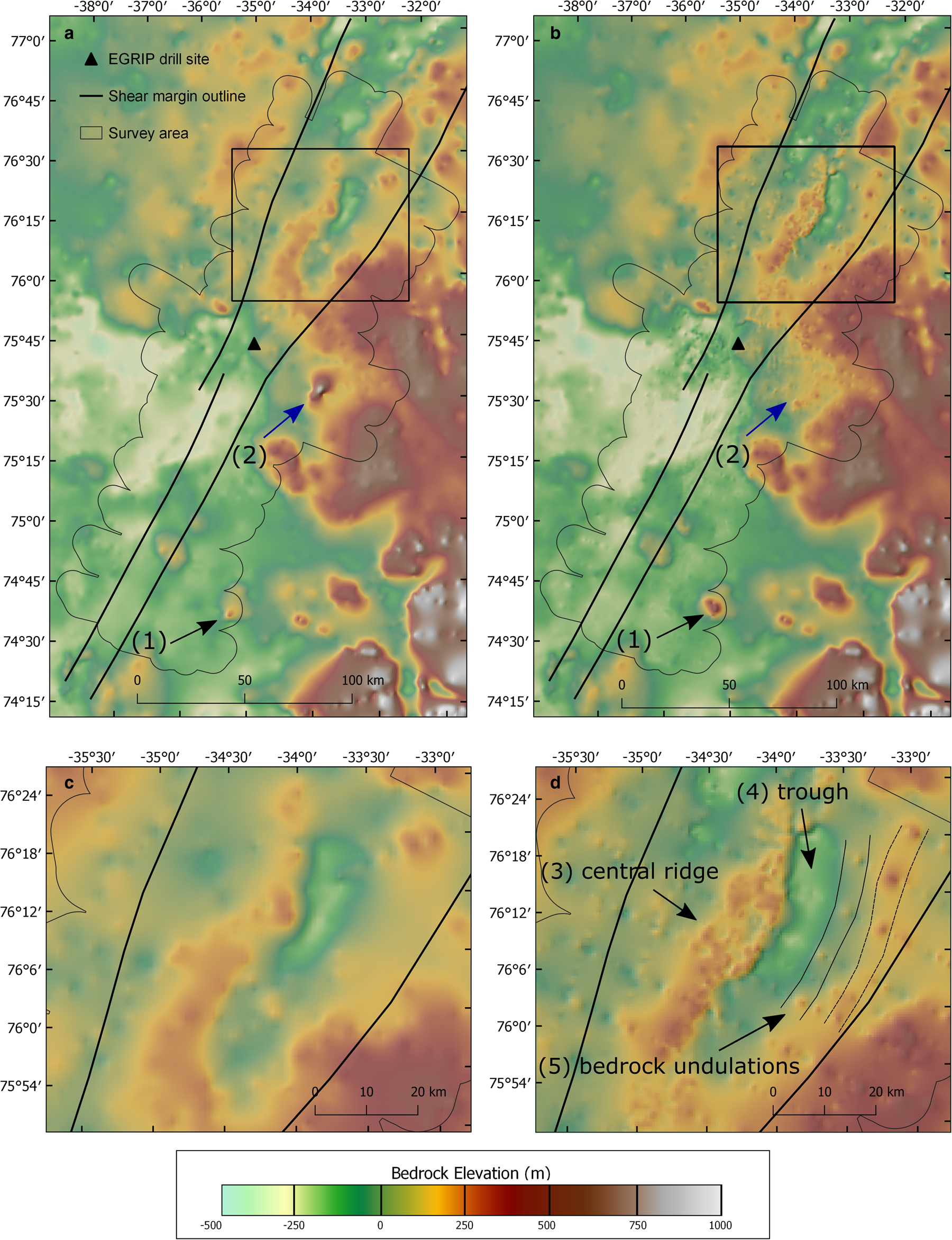
Fig. 3. Bed topography of (a) BedMachine v3 (Morlighem and others, Reference Morlighem2017 and (b) the EGRIP-NOR-2018 bed topography derived from our ice thickness data. A magnified view for the area upstream of the EGRIP drill site for both models (a and b) is shown on the two lower images (c and d, respectively). Two locations with strong elevation differences are marked with a black and blue arrow (feature 1 and 2). In the magnified sections, (c) and (d), we show the location of features 3–5. The black lines in feature 5 outline a possible connection of the single undulations.
In comparison with the BMv3 bed the most prominent differences of our bed topography appear at different locations and show five main features:
(1) Figures 2b and 3a and b show a location with elevation differences as large as 367 m. This isolated hill in the southeast of our survey area (indicated with a black arrow in Figs 3a and b) shows a higher basal elevation and larger surface area in the EGRIP-NOR-2018 topography in comparison with BMv3.
(2) A hill in the central southeast of our survey area, which is visible in the BMv3 bed topography (Fig. 2b and marked with a blue arrow in Figs 3a and b) and roughly 20 km away from the eastern shear margin, is not present in our bed topography. At this position, we find no significant change in ice surface topography but a strong internal reflection above the bed (Fig. 4). The highest elevation of BMv3 at this point is 697 m higher than our bed elevation. Three survey lines cover this feature and reveal strongly folded isochrones in our echograms. An internal anticline extending up to 15 km along the track exhibits elevation differences of isochrones of more than 900 m (Fig. 4). Furthermore, this radargram shows a strong power return of a similar amplitude as the bottom reflector in the proximity of the anticline. This reflection is irregularly shaped with interruptions, steeply dipping flanks and shows multiple layering. Underneath this anticline, we observe a weaker reflection, which we interpret as the real bed echo.
(3) A longitudinal ridge in the center of the ice stream 35–90 km downstream of the EGRIP drill site is located 300–500 m higher than the surrounding bed. In contrast to BMv3, this topographic high is now represented as being more isolated from the high elevated area in the east, that coincides with the position of the eastern shear margin on its western edge. The ridge is oriented only a few degrees off from the direction of the surface ice flow of the NEGIS.
(4) Southeast of the ridge, we find a trough. The transition is marked by a high elevation gradient of up to 500 m over a distance of 2–5 km. The trough shows an increasing depth in the along-flow direction and ends abruptly with a 300 m elevation increase over a distance of 3 km.
(5) Further east of the trough our radar lines show isolated bed undulations, which are aligned in the ice flow direction and bend downstream toward the western shear margin. The shape of this alignment is similar to the eastern and western slope of the trough to the West.
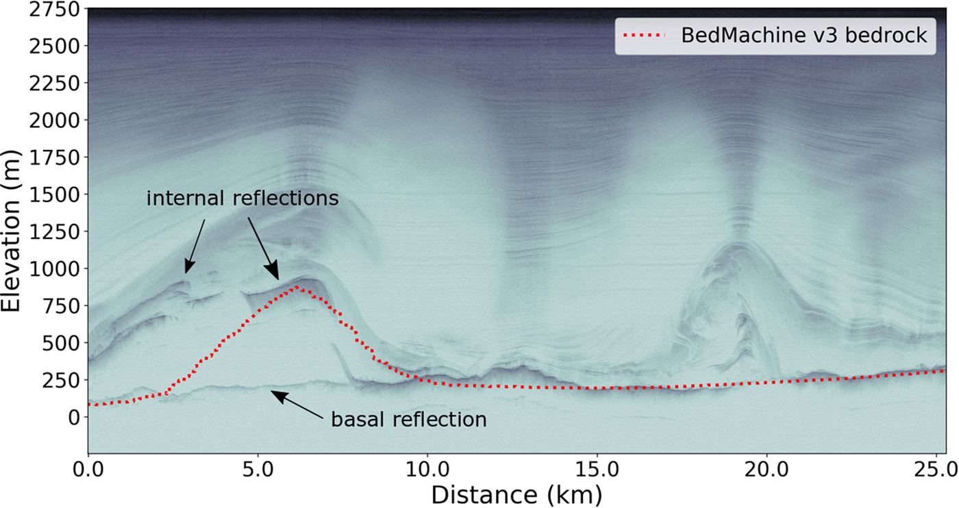
Fig. 4. Echogram from profile 20180508_06_003 along the point of our largest deviation in ice thickness (blue mark in Fig. 2). The dashed red line represents the bed elevation as used in BedMachine v3 (Morlighem and others, Reference Morlighem2017). The high peak at 6 km distance along the profile and ~750 m elevation correlates with a high energy internal reflection located in an area of folded internal layers. Underneath that undulation a fainter laterally straight and coherent reflection with a lower amplitude is visible, which we interpret as the basal reflection.
Discussion
Large scale bed structures
The EGRIP-NOR-18 bed topography shows several structures which are not present in previous bed elevation models. This is mainly due to our increased density in line spacing than in former surveys. Previous radar survey lines by AWI and Operation IceBridge (OIB) only covered parts of our survey area. At feature (1) in Figures 3a and b, only the edge of the bed feature was covered by one former survey line. However, the profile lines of other surveys indicate that this structure does not extend further than 10 km to the East. Feature (2) in Figure 3a is an ice bottom tracking error resulting from a strong reflection that does not represent the ice–bed interface (see Fig. 4).
Except for these larger scale differences between previously available datasets, the new nested bed elevation model mainly differs by more definition and steeper topographic gradients afforded by the increased spatial resolution of our data. The steeper gradients stand out in the region downstream of the EGRIP drill site, where a ridge in the center of the ice stream and an adjacent trough toward the east are delineated by a 300 m drop in bed elevation over 2 km. These structures are oriented almost parallel to ice flow (labeled with 3 and 4 in Fig. 3d). Further toward the east, the trough is bordered by a chain of bed undulations, which very likely form a connected ridge (Fig. 3d, features labeled 3, 4 and 5), also orientated roughly along ice flow. However, due to the lack of flow-parallel survey lines in this region this remains speculative. The trough shows the characteristics of an elongated, closed topographic depression: an overdeepening. These are common features in formally glaciated landscapes, and have been also documented underneath existing ice sheets and glaciers (e.g. Cook and Swift, Reference Cook and Swift2012; Patton and others, Reference Patton, Swift, Clark, Livingstone and Cook2016). A section of the bed along a flow line shows the typical profile of an overdeepening over two terraces, with the deeper part shifted toward the head (upstream) and a gentler upward slope downstream in each part of the basin. This indicates ongoing erosion by quarrying on the upstream end, leading to further deepening (Cook and Swift, Reference Cook and Swift2012). This geomorphology is usually more common toward the margins of the ice sheet, where large, fast-flowing outlet glaciers drain through confined valleys. Patton and others (Reference Patton, Swift, Clark, Livingstone and Cook2016) suggested that the overdeepening structures found in their analysis of the bed topography beneath the central part of the Antarctic and Greenlandic ice sheets might have been initiated in a period with a thinner ice layer, when the ice flow was more defined by the basal topography. The unusually high surface velocities of NEGIS, at least for the central region of the ice sheet, appear to facilitate ongoing erosion of the previously existing bed morphology. Patton and others (Reference Patton, Swift, Clark, Livingstone and Cook2016) also suggest that sedimentation of eroded material at the downstream end of the overdeepening would lead to a stabilization of the structure, preventing erosion downstream due to the softness of the sediment layer and thus, protecting the bed. This would then also result in the flattening of the surface profile. In case of the NEGIS there is a distinct step in the surface elevation at the downstream boundary of the basin, which might be interpreted as the erosion material being effectively flushed away.
As noted before by Christianson and others (Reference Christianson2014), the position and shape of the ice stream cannot be directly linked to the bed topography. The widening of the ice stream from a narrow channel with a width of 15 km upstream of the EGRIP Camp to a more than 50 km wide stream at the downstream end of our survey area is coincident with a 300 to 500 m step in the topography aligned perpendicular to the flow direction.
Interpretation of off-nadir reflections
For the major part of the survey area, the bed shows a clear reflection signature. Survey lines oriented transverse to ice flow show a variable bed topography with frequent elevation changes. Radargrams parallel to ice flow show a smooth and straight basal reflection. Elevation changes appear as elongated steps rather than a pattern of ridges and troughs. Several of the along-flow radargrams show off-nadir events underneath the initial bed reflection (Fig. 5). These events are only found in survey lines from within the ice stream. We interpret them to likely be caused by side reflections off-nadir, that is by elevation changes in the across-track dimension. Figure 6 shows a sketch of what kind of structures along the flight direction could generate these reflections in the radargrams. In some cases, we detect reflections in the form of straight lines, almost parallel and very similar to the shape of the primary bed reflection (subfigures 1, 2 and 3 in Fig. 5). These features are too close to the primary bed event to represent multiple reflections. We argue that the topography in these areas shows elongated ridges oriented parallel to ice flow, which are not visible in the large-scale topography of Figure 3 because of a lack of adequate spatial coverage and data point density. Considering the geometry of the radar beam and the footprint at the base of the ice sheet, the multiple reflectors could be generated by ridges with a height difference of tens of meters, and a ridge-to-ridge distance in the range of a hundred meters. However, on the basis of our data, this can only be evaluated qualitatively. These off-nadir reflection signatures are absent at the upstream end of our survey area, where ice-sheet velocity is below 30 m a−1. They become more pronounced with increasing velocity in the downstream area, approximately around the EGRIP camp, where the ice stream begins to widen. They appear in the western trough as well as on the central ridge. Unfortunately, there are no flow-parallel survey lines along the overdeepening in the east, so we cannot determine their presence. The structures have a length of up to 10 km (feature (1) in Fig. 5A). It is possible that the ridges extend even further, as the flight trajectory might not be exactly parallel to the orientation of the structures, which would cause a fading of the reflections in the radar data and thus interruptions in their appearance. In most cases the main bed reflection along these features is very smooth, at constant depth or with a very gentle slope, while at the downstream end of the multiple reflections a significant change in the bed slope can be detected (Figs 5A and B). This indicates that the flight line here is cutting the grooved bed at a small angle. Thus, it is not possible to derive the exact along-flow extension of these features from the airborne data, but we can only provide a lower estimate.
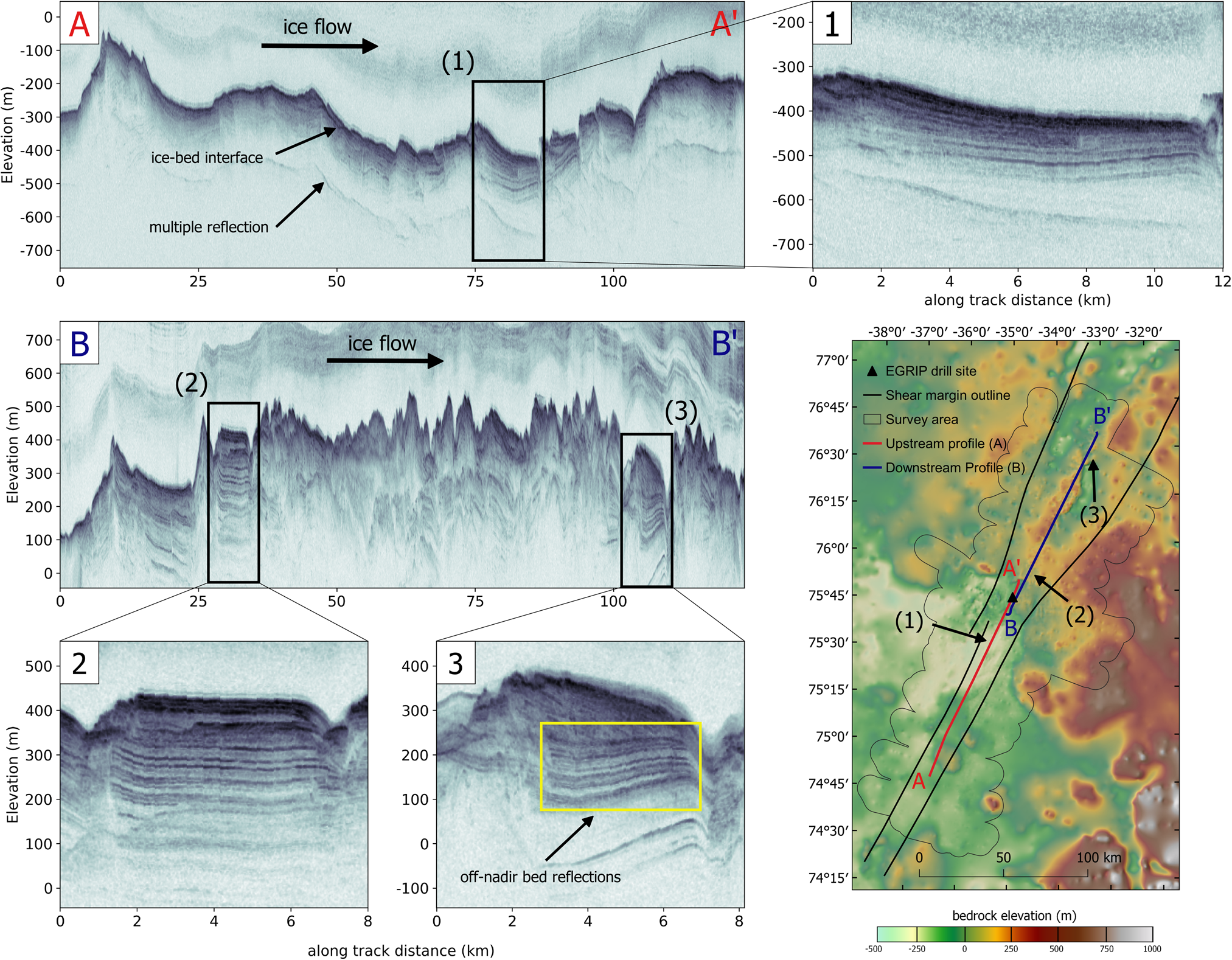
Fig. 5. A set of radargrams from the upstream (A) and downstream part (B) of the survey area oriented parallel to ice flow. The data were recorded with an increased radar cross-track beam angle. Subsections of the radargrams indicating the location of off-nadir reflections are shown in the radargrams 1, 2 and 3. An example of the off-nadir bed reflection pattern in the radargram is indicated in radargram 3 with the yellow outline. The position and the orientation of the radargrams (A to A′ in red and B to B′ in blue) as well as the location of the off-nadir reflection patterns 1, 2 and 3 are indicated in the map in the lower right corner.
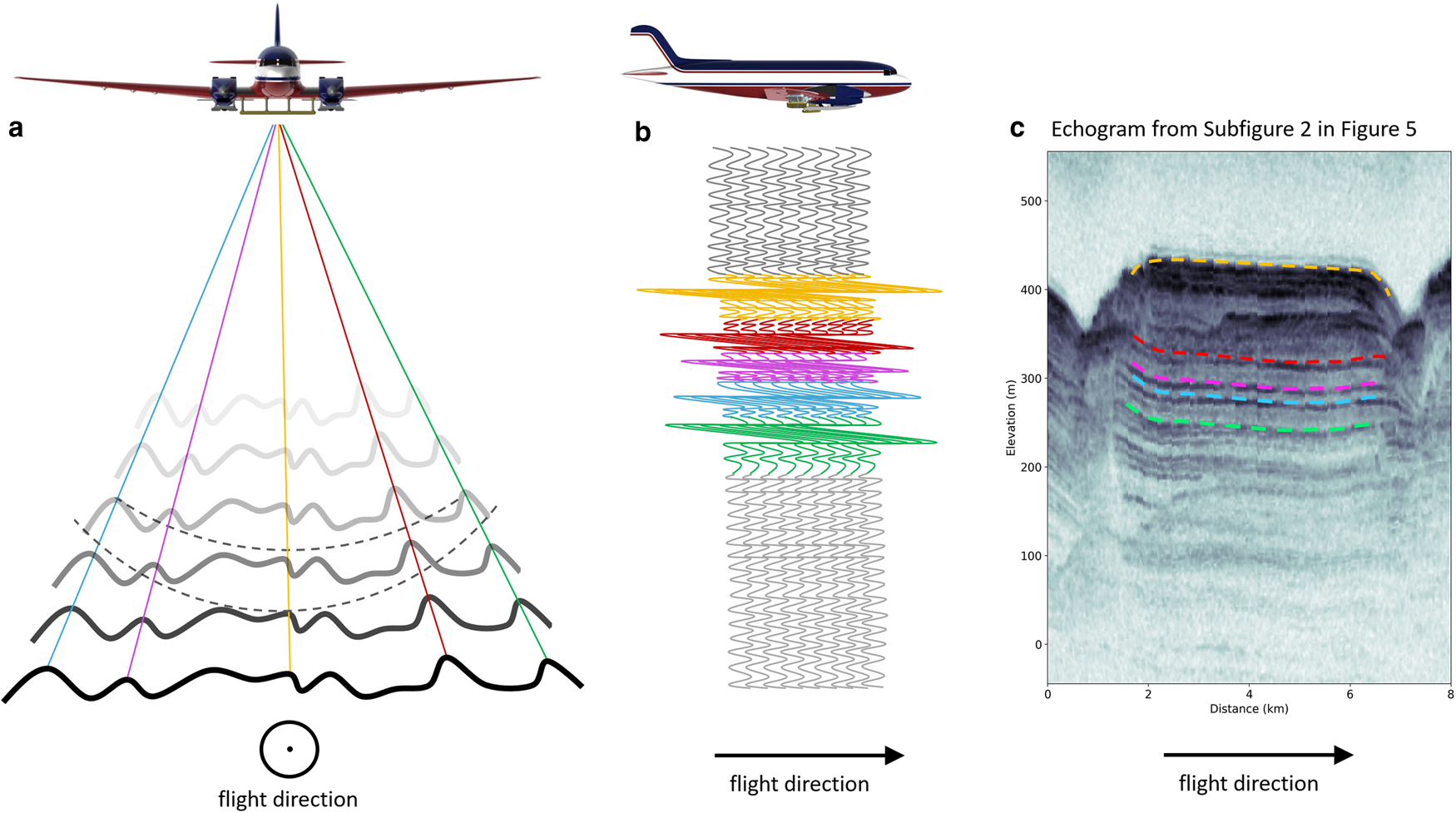
Fig. 6. This sketch shows how the bed structures of our interpretation of basal off-nadir reflections can look like. (a) Side reflections are scattered toward the receiver from elongated landforms aligned parallel to the flight trajectory. The black lines represent the bed reflector at different positions along the flight path. The different off-nadir reflections, which are most likely caused by scattered reflections by the elongated structures, are shown here in five different colors. (b) If the structure is parallel to the flight direction, a similar reflection pattern is recorded in the traces along the flight trajectory. (c) In the example of echogram section of the profile 20180515_01_007, the recorded signal could potentially look as indicated by the colored dashed layers. Plane model by courtesy of University of Kansas, Department of Engineering (2015).
The small-scale subglacial elongated landforms, which we deduce from the interpretation of side reflections, are probably a result of the flow activity of NEGIS in its current configuration, as they are parallel to the direction of observed surface ice flow. Elongated ridges at the ice–bed interface of a similar scale have been mapped underneath active ice streams before. Holschuh and others (Reference Holschuh, Christianson, Paden, Alley and Anandakrishnan2020) used swath radar data at Thwaites Glacier in Antarctica and mapped subglacial landforms which show a clear link between bedform orientation and ice flow. Jezek and others (Reference Jezek2011) interpreted ridges underneath parts of the Jakobshavn Isbræ as linear erosion of a hard bed, a landform which is also known from previously glaciated areas (Bradwell and others, Reference Bradwell, Stoker and Krabbendam2008). To create these structures high flow velocities and a significant sliding between ice and bed is required. However, data from a seismic survey close to the EGRIP Camp indicate a layer of soft, water saturated sediments beneath the main trunk of the ice stream. Saturated deformable sediments are one facilitator of fast-flowing ice streams (Winsborrow and others, Reference Winsborrow, Clark and Stokes2010) which can produce elongated bedforms, such as MSGL (Stokes and Clark, Reference Stokes and Clark2002). Apart from areas with relict MSGLs, they have also been documented beneath active ice streams, for example in West Antarctica below the Rutford Ice Stream by King and others (Reference King, Hindmarsh and Stokes2009), as well as below Pine Island Glacier (Bingham and others, Reference Bingham2017). MSGLs may be produced by either rapid ice flow over a short time, or slower ice flow over a longer duration (Stokes and Clark, Reference Stokes and Clark2002). We observe our features in areas of slow to moderate ice surface flow velocities of 30–80 m a−1 (based on surface velocities provided by Joughin and others, Reference Joughin, Smith and Howat2018). This would indicate that these subglacial features can either form at lower flow velocities or that ice flow in this region has persisted for a long time or at higher velocities than at present, and that dilatant till is present over a wide area beneath the ice stream. It is also possible that there are transitions between hard-bedded eroded streamlined landforms to soft-bedded landforms caused by different basal lithologies or a changing dynamic activity over several glacial cycles. Without further evidence about the nature of the ice–bed interface this remains speculative.
Conclusion
A new high-resolution ice thickness dataset has been computed on the basis of airborne radar data. We derived a bed elevation model and analyzed topography related structures in the area of the NEGIS in the vicinity of the EGRIP drill site. Basal topography is resolved in greater detail than in current bed elevation models of Greenland and covers a greater area than previous investigations and identified several misinterpretations of earlier ice thickness and thus bed elevation data. The enhanced resolution and more accurate geometry of the bed topography influences estimates of hydropotential and basal water routing. We observe an elongated topographic overdeepening, which indicates long-term erosion, potentially even over multiple glacial cycles. Small-scale elongated subglacial landforms in the center of the ice stream oriented parallel ice flow probably cause off-nadir reflections in our radargrams. Due to the survey line spacing and without additional geophysical data, the nature and geomorphology of these structures cannot be determined further. Either these landforms are formed by erosion in hard bed or by depositional processes, in which case they could represent MSGLs. The latter would also be consistent with the observations of Christianson and others (Reference Christianson2014), who found a meter thick layer of sediment across the ice stream located in the vicinity to the locations where we identify these features. Another set of seismic profiles and a higher resolution of the bed topography in regions where we interpret our basal radar return as subglacial landforms would be helpful to evaluate our hypothesis in terms of the composition and structure of elongated bedforms and the existence of sediments. However, a full 3-D bed elevation model is basically a requirement to more comprehensively interpret areas where we find evidence for the types and formation subglacial landforms. Nevertheless, our current analysis significantly improves previous bed elevation dataset in terms of coverage and accuracy, thus fostering more reliable ice flow model applications to investigate driving ice-dynamic process of NEGIS.
Data
The gridded ice thickness and bed topography data as well as the TWTs of the ice thickness along the radar profiles are available at the Data Publisher for Earth & Environmental Science (PANGAEA: https://doi.pangaea.de/10.1594/PANGAEA.907918).
Acknowledgments
We thank the crew of the research aircraft Polar 6. Logistical support in the field was provided by the East Greenland Ice-Core Project. EGRIP is directed and organized by the Center of Ice and Climate at the Niels Bohr Institute. It is supported by funding agencies and institutions in Denmark (A. P. Møller Foundation, University of Copenhagen), USA (U.S. National Science Foundation, Office of Polar Programs), Germany (Alfred Wegener Institute, Helmholtz Centre for Polar and Marine Research), Japan (National Institute of Polar Research and Arctic Challenge for Sustainability), Norway (University of Bergen and Bergen Research Foundation), Switzerland (Swiss National Science Foundation), France (French Polar Institute Paul-Emile Victor, Institute for Geosciences and Environmental research) and China (Chinese Academy of Sciences and Beijing Normal University). We acknowledge the use of software from CReSIS generated with support from the State of Kansas, NASA Operation IceBridge grant NNX16AH54G, and NSF grant ACI-1443054. The authors would like to thank Emerson E&P Software, Emerson Automation Solutions, for providing licenses in the scope of the Emerson Academic Program. We thank Martin Siegert and two anonymous reviewer for comments that improved the quality and readability of this manuscript.
Author contributions
Steven Franke wrote the manuscript and conducted the main part of the data processing and analysis. Olaf Eisen and Daniela Jansen were PI and Co-I of the campaign and designed the study. Daniela Jansen coordinated and conducted the field work together with Tobias Binder and John Paden. Veit Helm processed GPS data and assisted with further data processing together with Daniel Steinhage. John Paden and Nils Dörr contributed to the radar data processing with the CReSIS Toolbox and implemented the set-up for the nested bed elevation model. Daniela Jansen, Steven Franke and Olaf Eisen interpreted the radar and bed topography data. All co-authors discussed and commented on the manuscript.
Appendix A
Radar data processing
As a preliminary result, which is also generated in the field, we produce a quick look echogram with presumed unmigrated data. This output is used to automatically determine the ice surface location by using a maximum power layer tracker. CReSIS SAR processing algorithms use the surface location to model the ice as a layered media for fk migration (Leuschen and others, Reference Leuschen, Gogineni and Tammana2000). A simple dielectric half-space is used for representing the layered media with a relative dielectric permittivity of ice of 3.15. Recorded radar signals of each channel are processed individually and stacked coherently, equivalent to beamforming toward nadir. Depending on the number and pulse duration of the transmitted waveforms, different receiver gains are applied to increase the dynamic range. Radargrams with low and high gain are combined into a single image. The low gain echogram is used for the upper part of the image and the high gain echogram is used for the lower part of the image.
Pulse compression in the frequency domain is used to improve range resolution and SNR. As a result of this processing step, range sidelobes appear on both sides of the main return with a time window of twice the pulse duration (Li and others, Reference Li2013). A Hanning window is applied in the frequency domain to suppress range sidelobes and both the transmit signal and the matched filter are tapered with a Tukey window in the time domain. Range resolution depends on the propagation speed of the radar wave, and thus on the real part of the relative permittivity ɛr, the bandwidth of the transmitted chirp B and a factor for window widening due to the frequency and time domain windows, k i, according to
For the NB bandwidth of 30 MHz, the theoretical range resolution in ice with ɛr = 3.15 and k i = 1.53 is 4.31 m.
Transmit equalization
Prior to the data acquisition, transmit equalization of the emitted radar signals was performed on open water on the transit to Greenland. Adjustment of coefficients for amplitude, phase and time delay for each transmitter and each receiver helps to compensate any mismatches caused by hardware. This adjustment is of particular importance for beam-focusing and array processing to increase SNR. The coefficients are determined during a test flight prior to the actual data acquisition.
Motion compensation
Fourier-based processing algorithms for SAR processing require a uniformly sampled linear trajectory of the receivers along the extent of the SAR aperture and high precision timing information. Any deviation from a straight line reduces the maximum possible SNR of the received signal and induces phase errors, which degrade the target focusing (Legarsky and others, Reference Legarsky, Gogineni and Akins2001). Velocity variations, for instance, alter the along-track sampling and create an irregular sample spacing. High precision processed GPS and INS data from the aircraft are used to correct these effects. Before SAR processing, we (1) resampled the data in along-track using a windowed sinc interpolation kernel and (2) corrected any flight path deviations with a time delay.
SAR processing
The energy of radar wave reflectors spreads over a hyperbola in the along-track dimension produced by off-nadir reflections. The straight trajectory over the synthetic aperture length with uniform sampling points allows us to use frequency-wavenumber (fk) migration to locate reflection energy back to the target location. The technique is based on the fk-migration for seismic data (Gazdag, Reference Gazdag1978) and was adapted for radioglaciology (Leuschen and others, Reference Leuschen, Gogineni and Tammana2000). The processing uses signal information from adjacent traces and the result is based on the dielectric model of the subsurface to determine the radar wave propagation speed (Legarsky and others, Reference Legarsky, Gogineni and Akins2001). For the migration we use a layered velocity model with two constant permittivity values (ɛ = 1 for air and ɛr = 3.15 for ice). The air–ice interface is determined with an automatic surface tracker on unmigrated data. Time delays occurring due to changes of the aircraft trajectory and altitude are also corrected during this step (Rodriguez-Morales and others, Reference Rodriguez-Morales2014). The SAR aperture length at each pixel is chosen to create a fixed along-track resolution of 2.5 m.
Array processing
Coherent combination of return signals in the cross-track dimension is applied to increase SNR and to reduce surface clutter. For our processing, the antenna array beam is steered toward nadir. Since surface clutter due to crevasses is not prominent in our data, we applied the ‘delay and sum’ method for channel combination. This algorithm uses multi-looking of ambient pixels of the image pixel that is combined followed by along-track decimation (Jezek and others, Reference Jezek, Wu, Paden and Leuschen2013). To multilook, the array processed output is power detected and then averaged with neighboring pixels. In this case, the averaging window is 5 range lines before and 5 range lines after the current range line, resulting in reduced signal variance or fading and a coarser resolution of 2.5 m × 11 = 27.5 m along track. An output is generated every 6 range lines so that the sampling or posting in the final image is 2.5 m × 6 = 15 m.
For our bed return, we consider a cross-track resolution for a typical rough surface σy, which is constrained by the pulse-limited footprint and is dependent on Hanning and Tukey window factors:
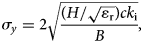
where H is the height of the aircraft over the ice surface and c the speed of light. Our flights were all performed at an elevation of ~365 m above ground, which corresponds to a cross-track footprint of 300–350 m for an ice column of 2000–3000 m in our survey region. The bed return, however, is in some cases characterized by layover signals from off-nadir due to topography. In this case, cross-track resolution depends on the full beam width, βy, of the antenna array:
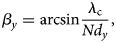
where λc is the wavelength at the center frequency, N is the number of array elements and d y is the element spacing of 46.8 cm. Cross-track resolution can now be calculated as
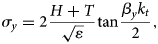
where T is the ice thickness and kt is the window widening factor which 1.53 for 20% Tukey time-domain window on transmit. Considering Eqn (A4) with a beam angle of ~21° corresponds to a cross-track resolution for the bed layer of 800 to 1100 m for an ice thickness range of 2000–3000 m.


 Open access