2.1. Application scenarios

In order to obtain the high-precision maps of large-scale scenes that don’t have their CAD models as ground truth, such as legacy nuclear facilities, historical heritage sites, chemical plants, etc, a novel methodology is proposed in this section. As shown in Fig. 1, the SLAM camera is firstly moved along a known ground truth trajectory (red solid arrow line), and the estimated trajectory (green dash arrow line) and the estimated map (chromatic point cloud) are generated based on the SLAM algorithm. Then the optimal error correction is calculated by minimizing the error between the ground truth trajectory and the estimated trajectory. This optimal error correction is then applied to optimize the estimated map to generate a high-precision map. Finally, the mapping error is evaluated by comparing the high-precision map with the ground truth map of the environment (here denotes the 3D model of the corridor available in benchmark). The proposed methodology is presented and detailed in Sections 2.2 and 2.3.

Figure 1. Concept of simultaneous localization and mapping benchmark and map accuracy improvement. The error correction minimizing trajectory errors is then applied to the estimated map to generate the high-precision map. One example of the potential applications is the mapping of a corridor.

2.2. Methodology of a comprehensive and objective SLAM benchmark

Compared with the current literature, the proposed novel benchmark methodology consists in benchmarking localization and mapping in a global coordinate system.

As shown in Fig. 2, a SLAM camera (RGB-D camera in the example) is used to map a 3D object (profile of a house in the example). To realize a comprehensive and objective SLAM benchmark, a high-precision measuring tool (e.g. VICON motion capture system) is needed for acquiring the ground truth of the trajectory and map, and a global coordinate system needs to be established so that the ground truth and estimates of the trajectory and map can be transformed into it for further evaluation.

As shown in Fig. 2(a), the trajectory ground truth $\boldsymbol{P}^{\mathrm{*}}$ and map ground truth $\boldsymbol{Q}^{\mathrm{*}}$ are acquired by using the high-accuracy vision system, working with a plurality of markers placed on the SLAM camera and object. The ground truth acquisition system is set up at a high position so that it can see all the markers, and its coordinate system is used as the global coordinate frame $\boldsymbol{G}$ . Several markers are placed at corners of the mapping object so that the ground truth mapping $\boldsymbol{Q}^{\mathrm{*}}$ can be obtained directly without any pose transformation.

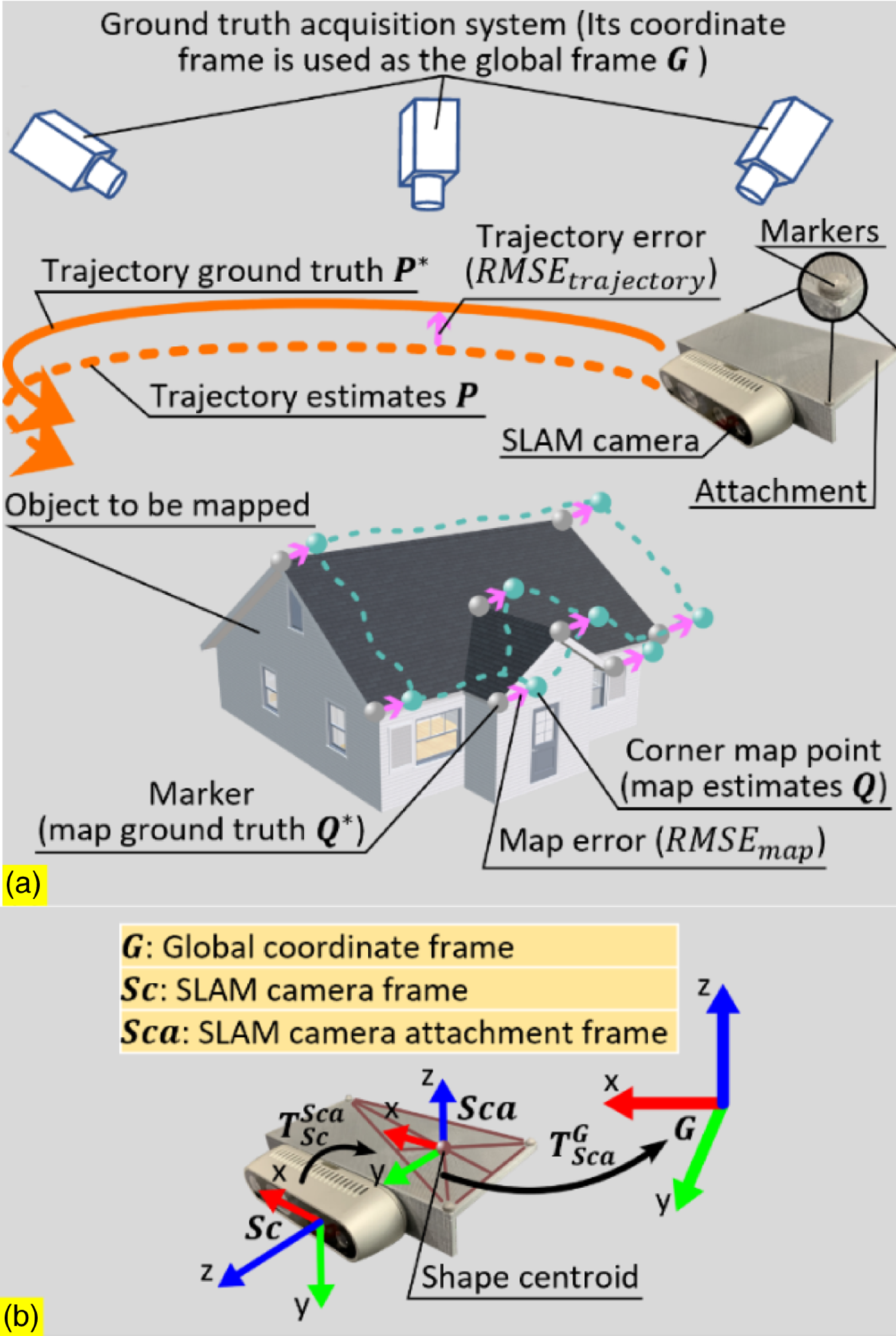
Figure 2. Schematic diagram of the benchmark methodology: (a) General concept of the methodology. To ensure the benchmark is comprehensive and objective, a high-precision measuring tool is used for ground truth acquisition, and its coordinate frame is used as the global frame, which all estimates and ground truth are transformed into. (b) Pose transformations between different frames. Except that the map ground truth $\boldsymbol{Q}^{*}$ can be obtained directly, the acquisition of the other three variables (map estimates $\boldsymbol{Q}$ , trajectory ground truth $\boldsymbol{P}^{*}$ , trajectory estimates $\boldsymbol{P}$ ) requires $Sca$ to achieve the transformation from their respective reference frames to the global frame $\boldsymbol{G}$ .

As shown in Fig. 2(b), the reference frame of the SLAM camera is denoted as $\boldsymbol{Sc}$ (SLAM camera frame), and the trajectory of its origin is considered as the SLAM camera trajectory. For acquiring the ground truth of the SLAM camera trajectory $\boldsymbol{P}^{\mathrm{*}}$ , a 3D-printed part is attached to the back of the SLAM camera with the attachment of three markers. The reference frame of these three markers is denoted as $\boldsymbol{Sca}$ (SLAM camera attachment frame); its origin is located at the centroid of the triangle encircled by the three markers, and its $x$ and $y$ axes are parallel to the attachment length and width respectively. $\boldsymbol{T}_{\boldsymbol{Sca}}^{\boldsymbol{G}}$ denotes the pose transformation from $\boldsymbol{Sca}$ to $\boldsymbol{G}$ ; it is being captured by the ground truth acquisition system constantly, and the position of $\boldsymbol{Sc}$ origin within $\boldsymbol{Sca}$ is a known factor; therefore, the ground truth of the SLAM camera trajectory can be obtained.

The markers on the SLAM camera attachment are placed in an asymmetric pattern, and the reason for this is that the symmetry of the rectangle encircled by four markers oftentimes obfuscates the ground truth acquisition system, which causes the pose of $\boldsymbol{Sca}$ to change during the operation. By contrast, the triangle encircled by three markers is asymmetric, which increases the robustness of the pose of $\boldsymbol{Sca}$ and makes it less likely to change during the operation.

The estimated trajectory and map obtained from the SLAM algorithm are originally within $\boldsymbol{Sc}$ , and the pose transformation from $\boldsymbol{Sc}$ to $\boldsymbol{Sca}$ is denoted as $\boldsymbol{T}_{\boldsymbol{Sc}}^{\boldsymbol{Sca}}$ which is also a known factor; therefore, the pose transformation from $\boldsymbol{Sc}$ to $\boldsymbol{G}$ can be expressed as $\boldsymbol{T}_{\boldsymbol{Sc}}^{\boldsymbol{G}}=\boldsymbol{T}_{\boldsymbol{Sca}}^{\boldsymbol{G}}\boldsymbol{T}_{\boldsymbol{Sc}}^{\boldsymbol{Sca}}$ . In this way, the estimated trajectory $\boldsymbol{P}$ and map $\boldsymbol{Q}$ within the global frame $\boldsymbol{G}$ can be obtained. In the global frame $\boldsymbol{G}$ , for all positions from the estimated camera trajectory $\boldsymbol{p}_{\mathbf{1}}$ , …, $\boldsymbol{p}_{\boldsymbol{n}}\in \boldsymbol{P}$ , their respective nearest neighboring positions from the ground truth trajectory are denoted as $\boldsymbol{p}_{\mathbf{1}}^{\mathrm{*}}$ , …, $\boldsymbol{p}_{\boldsymbol{n}}^{\mathrm{*}} \in \boldsymbol{P}^{\mathrm{*}}$ ; for all positions from the estimated map $\boldsymbol{q}_{\mathbf{1}}$ , …, $\boldsymbol{q}_{\boldsymbol{m}}\in \boldsymbol{Q}$ , their respective nearest neighboring points or mesh surfaces are denoted as $\boldsymbol{q}_{\mathbf{1}}^{\mathrm{*}}$ , …, $\boldsymbol{q}_{\boldsymbol{m}}^{\mathrm{*}} \in \boldsymbol{Q}^{\mathrm{*}}$ . For the camera trajectory, the nearest neighbor distance is point-to-point distance, and the Root Mean Squared Error (RMSE) overall nearest neighbor distances is expressed in Eq. (1). For the map, the nearest neighbor distance could be either point-to-point distance or point-to-mesh distance [Reference Cignoni, Rocchini and Scopigno26, Reference Aspert, Santa-Cruz and Ebrahimi27], and the RMSE of them is collectively expressed in Eq. (2). The RMSE is used as the evaluation metric for error analysis shown in Section 3.

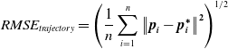(1) \begin{equation}RMSE_{\textit{trajectory}}=\left(\frac{1}{n}\sum _{i=1}^{n}\left\| \boldsymbol{p}_{\boldsymbol{i}}-\boldsymbol{p}_{\boldsymbol{i}}^{\boldsymbol\ast}\right\| ^{\mathbf{2}}\right)^{1/2}\end{equation}

(2) \begin{equation}RMSE_{map}=\left(\frac{1}{m}\sum _{i=1}^{m}\left\| \boldsymbol{q}_{\boldsymbol{i}}-\boldsymbol{q}_{\boldsymbol{i}}^{\boldsymbol\ast}\right\| ^{\mathbf{2}}\right)^{1/2}\end{equation}

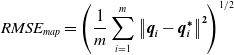
Figure 3. Workflow of the map accuracy improvement system. The approach used in the first step (trajectory error correction) is Centre Point Registration-Iterative Closest Point (CPR-ICP); it is subdivided into five substeps. The first four substeps constitute the CPR operation and are followed by the final ICP step. The output of CPR-ICP is a rigid transformation; it is fed into the step of map error correction and the revised high-precision map is obtained.

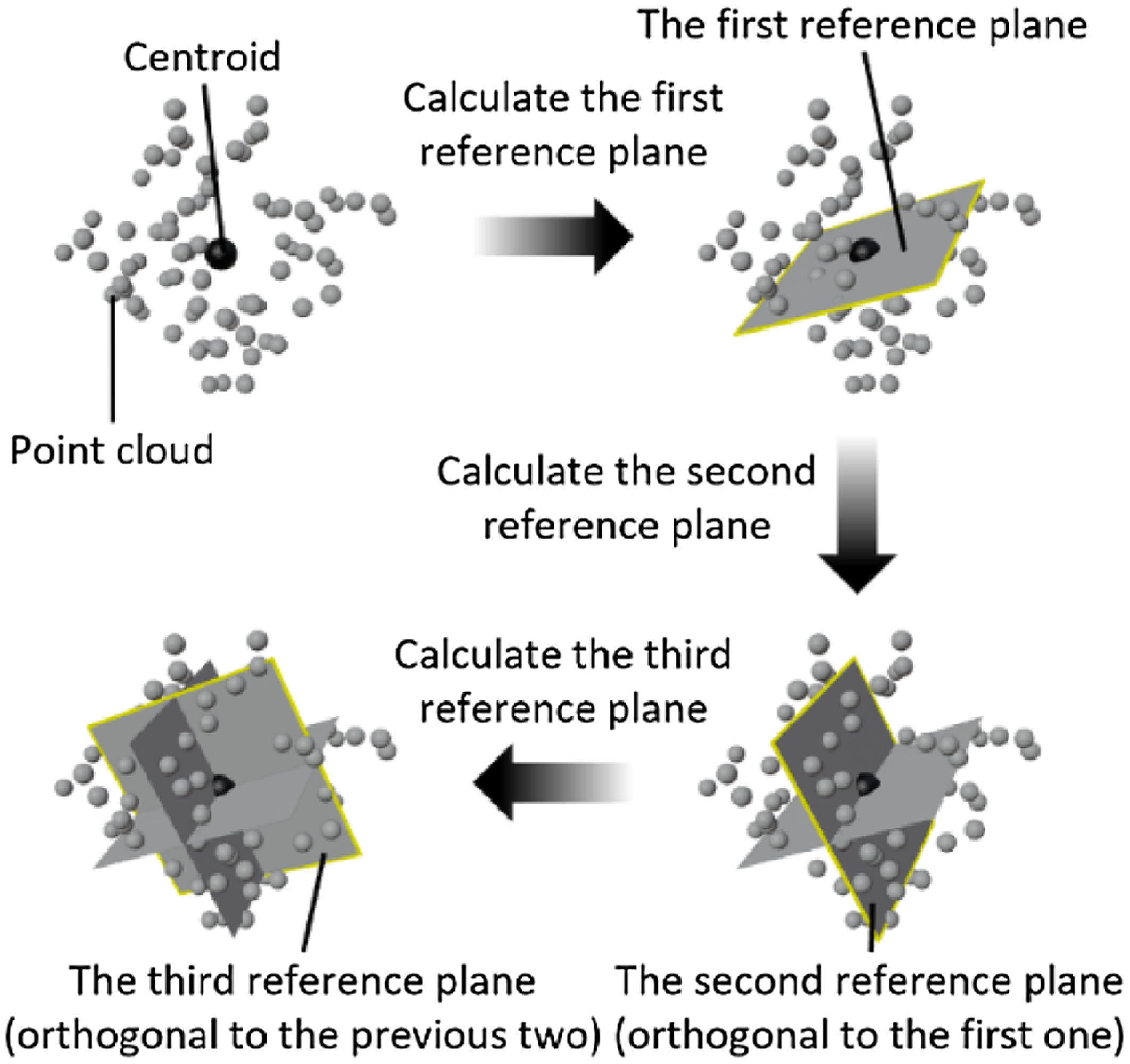
Figure 4. The objective of Centre Point Registration. Being orthogonal to each other, the three reference planes are fitted with the least squares method and they all pass through the centroid of the point cloud.

2.3. Methodology of map accuracy improvement

The motivation of the proposed novel methodology is to improve the accuracy of the estimated map in order to generate a high-precision map (geometry). As shown in Fig. 1, the novel methodology can be formulated as firstly finding the best error optimization between the estimated trajectory and ground truth trajectory and then applying this error optimization on the estimated map to obtain the high-precision map. The rationale behind this is that there exist correlations between the trajectory error and geometry error (yellow and pink curve double arrow lines). As shown in Fig. 3, the workflow of the map accuracy improvement system comprises two steps, that is trajectory error correction (Step 1) and map error correction (Step 2). The trajectory error correction is in essence the registration of the point cloud of the estimated trajectory (green point cloud) to the point cloud of the ground truth trajectory (red point cloud). The commonly employed approach is Iterative Closest Point (ICP) [Reference Besl and McKay19, Reference Arun, Huang and Blostein31–Reference Zhang33] method. For traditional ICP method, if there is no decent feature matching between two point clouds to start with, it cannot achieve good results. Therefore, a novel ICP, that is Centre Point Registration-ICP (CPR-ICP), is proposed to tackle this problem. The Centre Point Registration (CPR) is at the core of CPR-ICP and it is a pre-alignment process for the two point clouds prior to the ICP operation. The aim of CPR is to bring closer the same features in two point clouds and create a decent feature matching for the subsequent ICP operation to start with. As shown in Fig. 4, CPR is achieved by finding and aligning three reference planes for each point cloud, and the three reference planes should have the following attributes:

• • The first reference plane is achieved by minimizing the sum of the squares of distances between points and the plane.

• • The second plane has two attributes: (1) orthogonal to the first reference plane; (2) minimization of the sum of the squares of the distances between the points and the plane.

• • The third plane has three attributes: (1) orthogonal to the first reference plane; (2) orthogonal to the second reference plane; (3) minimization of the sum of the squares of the distances between the points and the plane is the minimum.

The problem of finding the three reference planes can be formulated in a mathematical way: given a point cloud $\boldsymbol{P}=\{\boldsymbol{p}_{\boldsymbol{i}}|\,\boldsymbol{p}_{\boldsymbol{i}}=[x_{i} y_{i} z_{i}]^{T}, i\in \mathbf{N }\cap i\in [1,n]\}$ and a plane $Ax+By+Cz+D=0$ with a unit vector of $\hat{\boldsymbol{u}}=[A B C]^{T}$ , the sum of the squares of the distances between the points and the plane can be expressed as:

(3) \begin{equation}f\left(\hat{\boldsymbol{u}},D\right)=\sum _{i=1}^{n}\left(\hat{\boldsymbol{u}}^{T}\boldsymbol{p}_{\boldsymbol{i}}+D\right)^{2}\end{equation}

Find the $\hat{\boldsymbol{u}}$ and $D$ that make (4) hold.

(4) \begin{equation}\lt \hat{\boldsymbol{u}},D\gt\,=min_{\hat{\boldsymbol{u}},D}f\left(\hat{\boldsymbol{u}},D\right)\end{equation}

If $f'_{\!\!D}(\hat{\boldsymbol{u}},D)=0$ , $D=-\hat{\boldsymbol{u}}^{T}\overline{\boldsymbol{p}}$ where $\overline{\boldsymbol{p}}=\frac{\sum _{i=1}^{n}\boldsymbol{p}_{\boldsymbol{i}}}{n}$ is the centroid of the point cloud $\boldsymbol{P}$ . This means that regardless of the normal unit vector $\hat{\boldsymbol{u}}$ , the planes making (4) hold definitely pass through the point cloud centroid $\overline{\boldsymbol{p}}$ (as shown in Fig. 4, all three reference planes pass through the centroid); therefore, the problem can be further formulated as: given a point cloud matrix $\boldsymbol{P}=[\boldsymbol{p}_{\mathbf{1}},\boldsymbol{p}_{\mathbf{2}},\ldots, \boldsymbol{p}_{\boldsymbol{n}}]$ where $\boldsymbol{p}_{\boldsymbol{i}}=[x_{i}\;y_{i}\;z_{i}]^{T}$ , $\overline{\boldsymbol{p}}=\frac{\sum _{i=1}^{n}\boldsymbol{p}_{\boldsymbol{i}}}{n}$ and $\mathbf{1}={[1,1,\ldots,1]_{\boldsymbol{n}\times \mathbf{1}}}^{T}$ , find the unit vector $\hat{\boldsymbol{u}}=[A\;B\;C]^{T}$ that makes (5) hold:

(5) \begin{equation}\hat{\boldsymbol{u}}=min_{\hat{\boldsymbol{u}}}\hat{\boldsymbol{u}}^{T}\left(\boldsymbol{P}-\overline{\boldsymbol{p}}\mathbf{1}^{T}\right)\left(\boldsymbol{P}-\overline{\boldsymbol{p}}\mathbf{1}^{T}\right)^{T}\hat{\boldsymbol{u}}\end{equation}

In (5), $(\boldsymbol{P}-\overline{\boldsymbol{p}}\mathbf{1}^{T})(\boldsymbol{P}-\overline{\boldsymbol{p}}\mathbf{1}^{T})^{T}$ is a symmetric matrix, so it can be factorized into the form of $\boldsymbol{U}\mathbf{\Sigma }\boldsymbol{U}^{T}$ using SVD (Singular Value Decomposition) [Reference Stewart34]; therefore, (5) can also be expressed as:

(6) \begin{equation}\hat{\boldsymbol{u}}=min_{\hat{\boldsymbol{u}}}\hat{\boldsymbol{u}}^{T}\boldsymbol{U}\left[\begin{array}{c@{\quad}c@{\quad}c} \lambda _{1} & 0 & 0\\[5pt] 0 & \lambda _{2} & 0\\[5pt] 0 & 0 & \lambda _{3} \end{array}\right]\boldsymbol{U}^{\boldsymbol{T}}\hat{\boldsymbol{u}}\end{equation}

In (6), $\boldsymbol{U}$ is an orthogonal matrix and $\lambda _{1}$ , $\lambda _{2}$ , $\lambda _{3}$ are the singular values and $\lambda _{1}\geq \lambda _{2}\geq \lambda _{3}$ ; therefore, $\boldsymbol{U}^{T}\hat{\boldsymbol{u}}$ is still a unit vector and can be denoted as $\hat{\boldsymbol{u}}^{\boldsymbol\prime}=[A'\;B'\;C']^{T}$ , so (6) can also be expressed as:

(7) \begin{equation}\hat{\boldsymbol{u}}^{\boldsymbol\prime}=min_{\hat{\boldsymbol{u}}^{\boldsymbol\prime}}\lambda _{1}A'^{2}+\lambda _{2}B'^{2}+\lambda _{3}C'^{2}\end{equation}

(7) holds if $\hat{\boldsymbol{u}}^{\boldsymbol\prime}=[0\;0\;1]^{T}$ , which means $\hat{\boldsymbol{u}}$ equals the last column vector of $\boldsymbol{U}$ ; therefore, the last column vector of $\boldsymbol{U}$ is the normal vector of the first reference plane. To find the second reference plane, the above calculation is repeated. Since the second reference plane also passes through the centroid and is orthogonal to the first reference plane, its unit vector $\hat{\boldsymbol{u}}^{\boldsymbol\prime}=[A'\;B'\;0]^{T}$ , so (7) reaches the minimum value $\lambda _{2}$ if $\hat{\boldsymbol{u}}^{\boldsymbol\prime}=[0\;1\;0]^{T}$ , which means $\hat{\boldsymbol{u}}$ equals the second to last column vector of $\boldsymbol{U}$ ; therefore, the second to last column vector of $\boldsymbol{U}$ is the normal vector of the second reference plane, and the first column vector of $\boldsymbol{U}$ is the normal vector of the third reference plane. To sum up, this calculation process firstly normalizes every point in the point cloud by the centroid, and then factorizes the square of the normalized point cloud matrix using SVD; therefore, the CPR operation can be elaborated as the following four steps:

1. 1. Compute the centroid (the mean of all point coordinates $\overline{\boldsymbol{p}}=\frac{\sum _{i=1}^{n}\boldsymbol{p}_{\boldsymbol{i}}}{n}$ ) of each point cloud and normalize each point cloud by the centroid, which is corresponding to Substep 1 of Step 1 shown in Fig. 3.

2. 2. Apply SVD to each normalized point cloud and compute the three normal vectors, which is corresponding to Substep 2 of Step 1 shown in Fig. 3.

3. 3. Translate the source point cloud (the estimate) to the reference point cloud (the ground truth) and align their centroids, which is corresponding to Substep 3 of Step 1 shown in Fig. 3.

4. 4. Rotate the translated source point cloud (the estimate) around its centroid and align its three normal vectors to those of the reference point cloud (the ground truth), which is corresponding to Substep 4 of Step 1 shown in Fig. 3.

3.1. Experiments of small-scale scenes

The proposed methodology is then tested on a small-scale SLAM scene. As shown in Fig. 6(a), in the experiment, a Vicon motion capture system is used for acquiring ground truth and providing global frame $\boldsymbol{G}$ ; a laptop (SLAM laptop) with an Intel Core i9-10980HK CPU (2.40 GHz, 8 Cores, 16 Logical Processors) and 32 gigabytes memory is used to run the SLAM algorithm ORB-SLAM2 [Reference Mur-Artal and Tardós38]; and an Intel RealSense D435i RGB-D camera is affixed at the top of the SLAM laptop and used as the SLAM vision sensor (SLAM camera). As shown in Fig. 6(b), the map being evaluated consists of three points that are centroids of three rectangular regions on a 75 × 75 cm table surface. The table surface is partitioned into four equal rectangular regions by tapes with color textures. Among the four rectangular regions, twelve markers are placed at the corners of three rectangular regions; in this way, the centroid coordinates (three blue points) of these three rectangular regions can be captured directly by the motion capture system and used as the ground truth map $\boldsymbol{Q}^{*}$ , as is shown in Fig. 6 (c). The ground truth map $\boldsymbol{P}^{*}$ , estimated trajectory $\boldsymbol{P}$ and estimated map $\boldsymbol{Q}$ are also shown in the form of point clouds in Fig. 6(c).

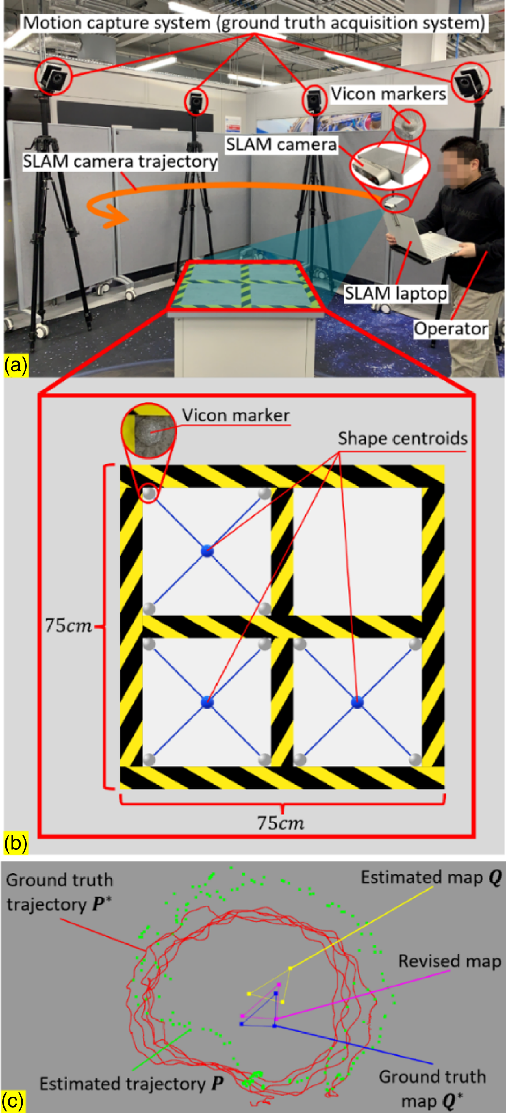
Figure 6. Experimental setup and operation of simultaneous localization and mapping benchmark and map accuracy improvement (SLAMB&MAI). (a) The SLAM system consists of an RGB-D camera (SLAM camera) and a laptop (SLAM laptop); the SLAM camera scans the table surface and feeds the image data into the SLAM laptop to generate the point cloud. During the scanning operation, the SLAM laptop is carried by an operator moving around the table surface, meanwhile, the pose of the SLAM camera is constantly adjusted by the operator to make sure the entire table surface stays in SLAM camera’s field of view and the SLAM camera attachment frame ( $\boldsymbol{Sca}$ ) stays in Vicon’s field of view throughout the operation process. After the scanning operation is done, all obtained coordinates are transformed into the global frame $\boldsymbol{G}$ . In the transformed map point cloud, the map points at four corners of the three rectangular regions are chosen manually, and their mean coordinate is used as the map estimate; then the errors of SLAM camera trajectory and map are calculated, and the error correction function of camera trajectory is obtained and applied to the map estimates to obtain the high-precision map. (b) The layout of the map setup on a table surface. (c) The point cloud of the captured data under the global coordinate frame $\boldsymbol{G}$ . The three blue points represent the ground truth map $\boldsymbol{Q}^{*}$ ; the three yellow points represent the estimated map $\boldsymbol{Q}$ ; the three purple points represent the revised map; the green points represent the estimated trajectory $\boldsymbol{P}$ ; and the dense red points represent the ground truth trajectory $\boldsymbol{P}^{*}$ .

During the experimental operation, the SLAM camera scans the table surface constantly to generate its point cloud; in the meantime, the pose of the SLAM camera attachment frame ( $\boldsymbol{Sca}$ ) relative to the global frame $\boldsymbol{G}$ is being captured constantly by the motion capture system so that $\boldsymbol{P}$ , $\boldsymbol{P}^{*}$ , $\boldsymbol{Q}$ and $\boldsymbol{Q}^{*}$ can be obtained within the global frame $\boldsymbol{G}$ using the pose transformations shown in Section 2. Within the generated point cloud of the table surface, for each rectangular region, the four map points at four corners are chosen manually and their coordinates are averaged, and these three mean coordinates are used as the estimated map $\boldsymbol{Q}$ (three yellow points). After $\boldsymbol{P}$ , $\boldsymbol{P}^{*}$ , $\boldsymbol{Q}$ and $\boldsymbol{Q}^{*}$ are obtained within the global frame $\boldsymbol{G}$ , for the purpose of benchmarks, the RMSE errors of the trajectory and map are calculated based on Eqs. (1) and (2). Then the error correction function CPR-ICP (obtained in Step 1 shown in Fig. 3) or traditional ICP can be obtained, it is applied on the estimated map $\boldsymbol{Q}$ and the revised map (three purple points) is obtained, as is shown in Fig. 1 and Step 2 in Fig. 3. Then, the RMSE errors between the revised trajectory and map and the ground truth trajectory and map are calculated as well based on Eqs. (1) and (2), respectively.

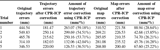
Table I. Errors of map and trajectory before and after Centre Point Registration-Iterative Closest Point correction for the small-scale scene.

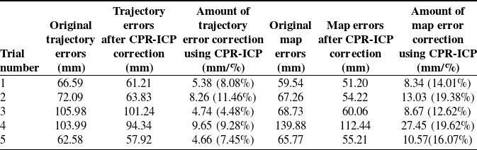
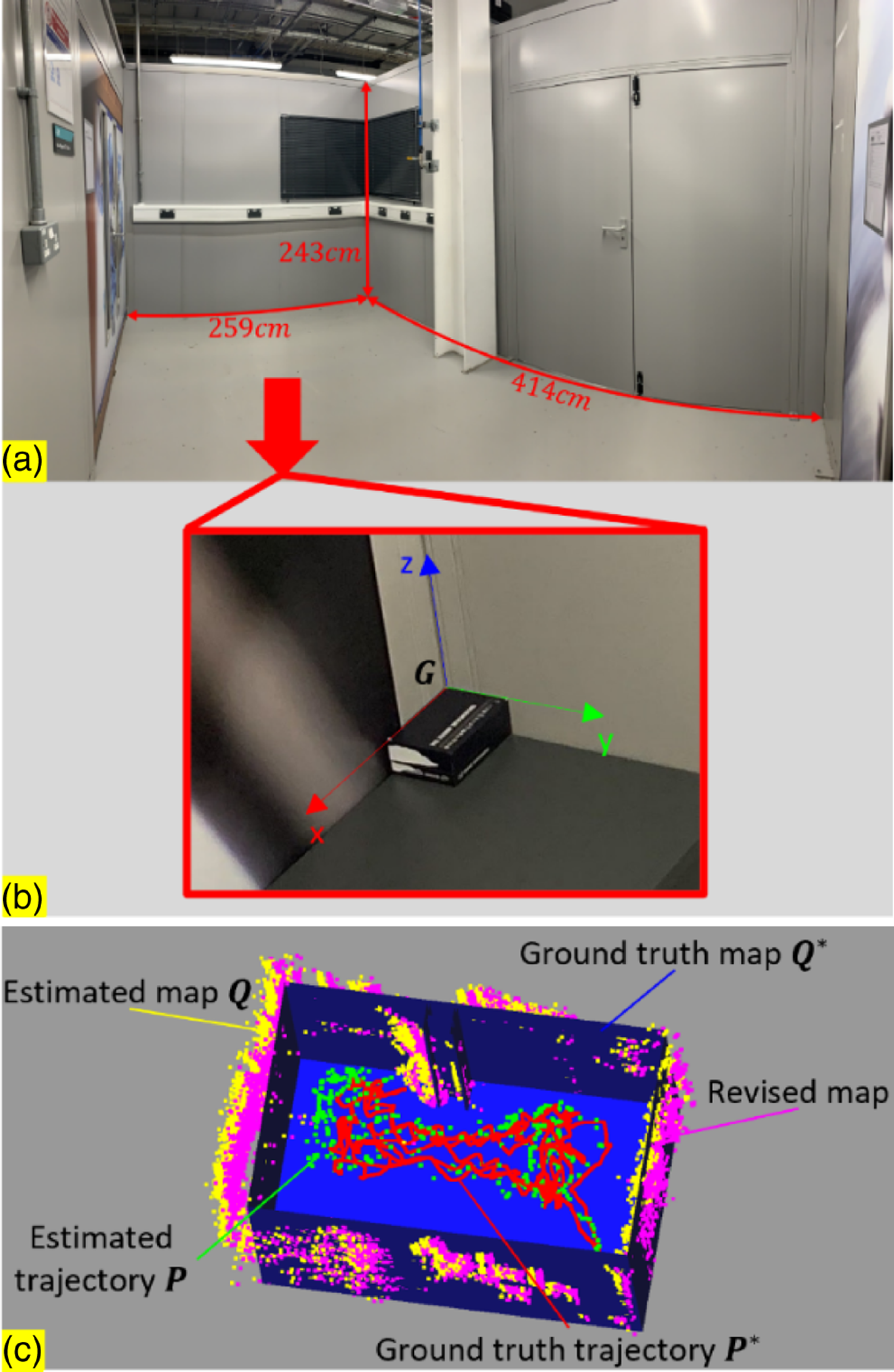
Figure 7. Experiment setup in medium-scale environments and results. (a) A panoramic photo of the medium-scale scene. (b) The global coordinate frame $\boldsymbol{G}$ was established at a corner where two walls meet, and its relative position to the small-scale room is known. (c) The point clouds of the ground truth and estimate of the camera trajectory and map. The blue CAD model represents the ground truth map $\boldsymbol{Q}^{*}$ , its relative position to $\boldsymbol{G}$ is known; the yellow point cloud represents the estimated map $\boldsymbol{Q}$ ; the purple point cloud represents the revised map; the green point cloud represents the estimated trajectory $\boldsymbol{P}$ ; and the dense red point cloud represents the ground truth trajectory $\boldsymbol{P}^{*}$ . They were all captured under the global frame $\boldsymbol{G}$ .

Table II. Errors of map and trajectory before and after Centre Point Registration-Iterative Closest Point correction for the medium-scale scene.

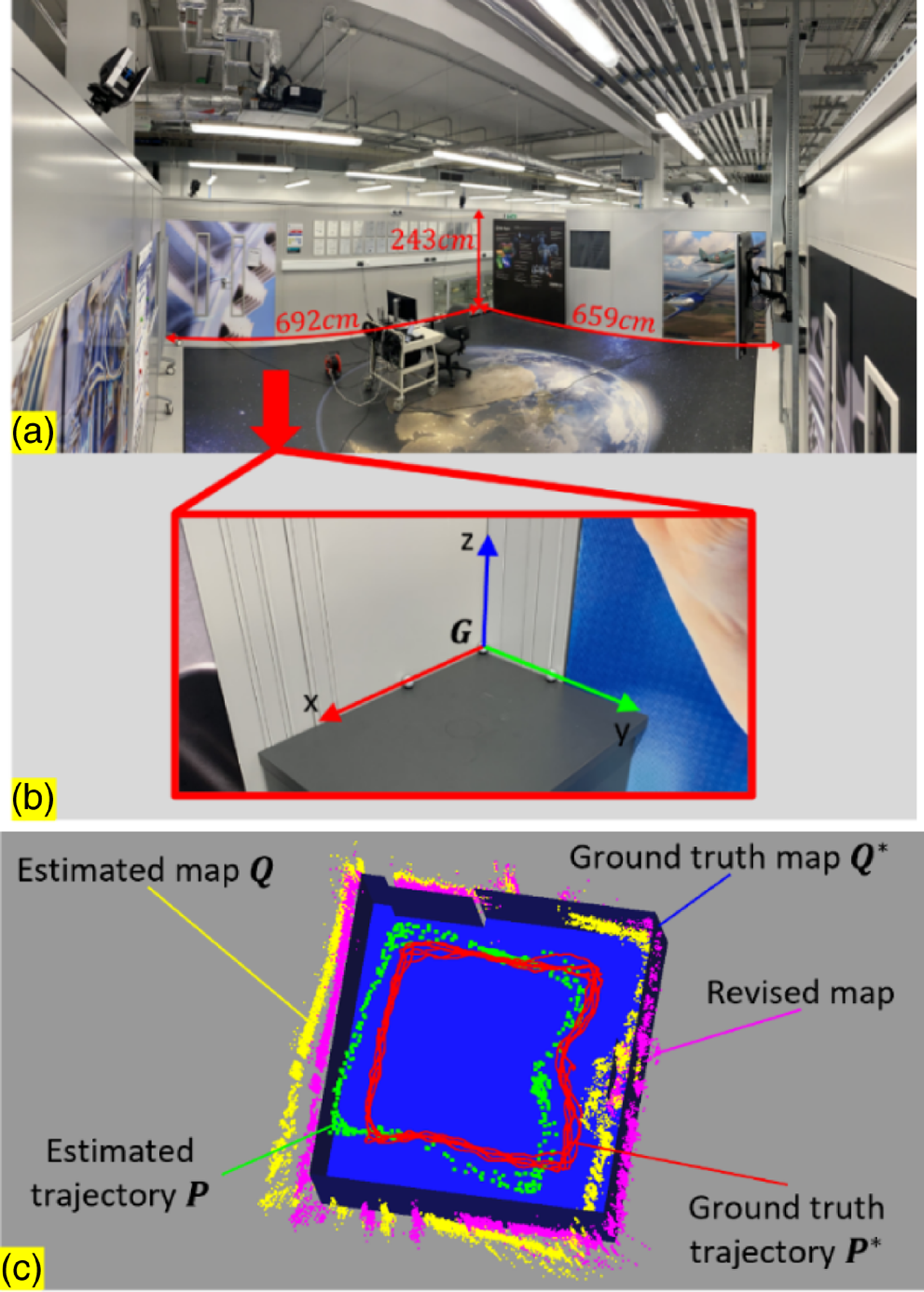
Figure 8. Experiment setup in large-scale environments and results. (a) A panoramic photo of the large-scale scene. (b) The global coordinate frame $\boldsymbol{G}$ is established at a corner where two walls meet, and its relative position to the small-scale room is known. (c) The point clouds of the ground truth and estimate of the camera trajectory and map. The blue CAD model represents the ground truth map $\boldsymbol{Q}^{*}$ , its relative position to $\boldsymbol{G}$ is known; the yellow point cloud represents the estimated map $\boldsymbol{Q}$ ; the purple point cloud represents the revised map; the green point cloud represents the estimated trajectory $\boldsymbol{P}$ ; and the dense red point cloud represents the ground truth trajectory $\boldsymbol{P}^{*}$ . They were all captured under the global frame $\boldsymbol{G}$ .

As shown in Table I, the test results show that the concept of correcting map errors using trajectory error correction works fine; it can reduce the map error by an average of around 15%. Among all test results, for either trajectory or map, ICP and CPR-ICP reduce roughly an equal amount of errors. The reason for this is that in the small-scale scene, the point clouds of estimates and ground truth tend to have a decent initial feature matching between them; therefore, the CPR correction makes a modest contribution. But for a point cloud registration case that doesn’t have a decent initial feature matching like the one shown in Fig. 5, the CPR correction makes a significant difference. To further verify the practical applicability of the proposed methodology for scenes with larger scales, experiments in a medium-scale scene and a large-scale scene were conducted and are detailed in 3.2 and 3.3, respectively.

3.2. Experiments of medium-scale scenes

Similar experiments were then carried out in a medium-scale room with the size of $243\,\rm cm\times 259\,\rm cm\times 414\,\rm cm$ , as is shown in Fig. 7(a). The captured data shown in Fig. 7(c) are similar to the one shown in Fig. 6(c), except that the ground truth map $\boldsymbol{Q}^{\mathrm{*}}$ is a manually drawn CAD model instead of a point cloud. The global frame $\boldsymbol{G}$ shown in Fig. 7(b) was established at a corner where two walls meet, and the relative position of $\boldsymbol{Q}^{\mathrm{*}}$ to $\boldsymbol{G}$ was pre-obtained by manual measurement. Using the manually drawn CAD model as ground truth map would introduce errors; therefore, the actual performance of the proposed methodology is better than the test results shown in Table II.

Table III. Errors of map and trajectory before and after Centre Point Registration-Iterative Closest Point correction for the large-scale scene.

As shown in Table II, the concept of correcting map errors using trajectory error correction also works for medium-scale scenes; the map error was reduced by an average of around 12%. As mentioned before, using the manually drawn CAD model as ground truth map would introduce errors, so it’s safe to say the proposed methodology is able to reduce the map error by at least 12%. Among all the test results, 40% of them of CPR-ICP are better than that of ICP, which is higher than the 20% for the small-scale scene. This result shows that CPR-ICP tends to outperform ICP in scenes with larger scales, so more experiments were conducted in a large-scale scene and are presented in the next section.

3.3. Experiments of large-scale scenes

The proposed methodology is then tested on a large-scale room with the size of $243cm\times 692cm\times 659cm$ as shown in Fig. 8. Same as the test in medium-scale scenes, using the manually drawn CAD model as ground truth map would introduce errors, so the actual performance of the proposed methodology is better than the test results shown in Table III.

As can be seen from Table III, the concept of correcting map errors using trajectory error correction works for large-scale scenes as well; the proposed methodology was able to reduce the map error by around 20%. Among all test results, 80% of them of CPR-ICP are better than that of ICP, and 40% are better by above 15%. Combined with the 0% for small-scale scenes and 40% for medium-scale scenes, the ratios of test results in which CPR-ICP is better than ICP in different scale scenes are shown in Fig. 9. As can be seen from Fig. 9, in terms of map error correction, the trend shows that the proposed CPR-ICP tends to outperform the traditional ICP in scenes with larger scale. The reason is that the SLAM 3D reconstruction of large-scale scenes tends to have more errors, therefore, a pre-alignment before ICP is necessary.

Figure 9. The ratios of test results in which Centre Point Registration-Iterative Closest Point (CPR-ICP) is better than ICP in different scale scenes. The trend shows that the proposed CPR-ICP tends to outperform the traditional ICP in scenes with larger scales.