1. Introduction

Synthetic-aperture-radar (SAR) data are an important source of information for investigations of the Greenland and Antarctic ice sheets, because the SAR signal penetrates the cloud cover. This is, for instance, not the case for advanced very high resolution radiometer (AVHRR) data, which are collected mainly for weather observations and climate studies.

Visual interpretation of SAR data is impeded by the distortion of the morphology that is typical of any side-scan radar or sonar device. Well-known satellite-image-analysis software developed for visual satellite imagery such as Landsat is not applicable, because the multivariate methods require several channels. Consequently quantitative analysis of SAR data necessitates new mathematical solutions. SAR data do not contain absolute reference of grey value and scale, and depend on on-look angle. This calls for mathematical methods that do not depend on an absolute value but on first-order differences.

A good example of such a method is interferometry, based on the phase difference of two consecutive images. If all other physical parameters remain constant during the time of collection of the two datasets, the phase difference may be used to calculate the velocity of a glacier (Reference Goldstein, Engelhardt, Kamb and FrolichGoldstein and others, 1993). Since phase difference is only a one-dimensional variable, inversion to only one other variable is possible, which necessitates the exclusion of any effect that may cause decorrelation of the images. An alternative is to model such effects first. If, however, the ice movement is too complex, interferometry is no longer applicable.

Examples are glaciers during a surge (Reference HerzfeldHerzfeld, 1998) and fast-moving ice streams, the prototype of which is Jakobshavn Isbræ in West Greenland. An interferogram showing lack of coherence on Jakobshavn Isbræ was available on the world-wide web (under Greenland investigations). Geostatistical ice-surface characterization is applied to investigate complex ice movement based on strain patterns rather than on velocity changes. Related principles derived from structural geology are explained and applied to photographic images of Jakobshavn Isbrs in Reference Mayer and HerzfeldMayer and Herzfeld (2000).

The method uses the variogram, the spatial-structure function most common in geostatistics, and as such is another example of a mathematical method that depends only on first-order differences of the data (considered a realization of a stochastic process) rather than on the data themselves, so absolutely referenced values are not needed in the analysis. The geostatistical surface classification system has been developed and applied to sea-floor data (Reference Herzfeld and HigginsonHerzfeld and Higginson, 1996) and to video data from ice surfaces (Reference HerzfeldHerzfeld, 1999). To establish a classification for a new data type, there are three steps of increasing complexity: First, homogeneous surface classes need to be identified and characterized quantitatively (characterization). Second, results from the characterization are used to assign objects that were previously unknown to the system to an object class; here, to relate a given ice-surface area to one of a number of ice-surface classes (classification). Third, a segmentation of an entire region may be obtained by application of the classification procedure as a moving-window operator to a large spatial dataset (segmentation).

In this paper we investigate the usefulness of European Remote-sensing Satellite (ERS) 1 and 2 SAR data for surface classification.

Due to their high resolution, about 30 m and 12.5 m pixel size, SAR data may also be considered a source of subscale information for the study of radar-altimeter data. Subscale variability is the amount of information that is lost in any survey due to the limited resolution of the instrument. In turn, video data or SAR data collected from aircraft may provide subscale information for satellite SAR data, and ground-truth data are needed for any kind of remote sensing data. However, the commonly used terminology "ground truth" does not necessarily imply a survey at higher resolution, but may refer to any type of field work. Such a survey requires special instrumentation.

A survey of surface-morphologic properties at 0.2 m × 0.1 m resolution on the ice surface was carried out with an instrument specifically designed for this purpose during expedition MIGROTOP’97, for selected areas and surface types in the Jakobshavn Isbræ drainage basin. Analysis of those data (Reference Herzfeld, Mayer, Feller and MimlerHerzfeld and others, 2000) serves as ground truth in the geostatistical characterization of SAR data. In this case, surface classes are morphological provinces.

2. Geostatistical Surface Characterization: Mathematical Background in a Nutshell

As mentioned in the introduction, the variogram is a spatial-structure function that depends only on first-order differences, or increments, of the data, considered as a realization of a stochastic process. This property is assured by the so-called "intrinsic hypothesis" (Reference MatheronMatheron, 1963). Elevation is considered a regionalized variable z(x) defined throughout a two-dimensional region D and characterized by a structural aspect and a random variation (Reference MatheronMatheron, 1963). Then z(x)satisfies the intrinsic hypothesis if [z(x)–z(x+h)] is second-order stationary. A consequence of the intrinsic hypothesis is that the variogram exists under conditions where the spectrum or the covariance functions do not exist. Because of this property the variogram is applicable to SAR data. The variogram is calculated as

where z(xz), z(xz + h) are samples taken at locations xi, xl + h ∊ D, respectively, and n is the number of pairs separated by h To detect a drift, the residual variogram is calculated as

where m(h) IS given by

The variogram is well-known as the structure function used in kriging, where a model is fitted to match the transitive behaviour typical of a regionalized variable (low-variogram values for short lags monotonously increasing to high-variogram values for long lags), and finally to solve for the kriging coefficients in the interpolation. For lags exceeding a certain distance, the variogram "fluctuates" around a sill value, indicative of the total variance. These fluctuations are the source of information in geostatistical characterization and classification (Reference HerzfeldHerzfeld, 1999) which is applied here to study and describe ice-surface roughness. Roughness characteristics are captured in parameters that are extracted from the experimental variogram, these parameters constitute a feature vector. For characterization, feature vectors need to be selected that describe an ice-morphological type or ice-surface class uniquely. For classification, feature vectors need to be selected such that each object encountered in a given area may be assigned uniquely to an ice-surface class from a given set of classes. Obviously it is necessary to first master the characterization problem before the surface classification problem can be approached.

The following parameters are applied in the ensuing study of SAR data. The mindist parameter is the lag of the first minimum after the first maximum in the variogram. The dirmin parameter is the direction in which the first minimum occurs first. For anisotropic systems resembling a hill-and-valley pattern, dirmin is the direction normal to the strike of hills. An example is a crevasse field, smoothed in its appearance in a SAR image by the remote-sensing process. To distinguish pure hill-valley sequences from overprinted ones and to characterize more complex morphologic structures, significance parameters are introduced:

p1 is the slope parameter and P2 the relative significance of the first minimum, mini, after the first maximum, max1, and h_× and γx denote lag and variogram value of x, respectively (Reference Herzfeld and HigginsonHerzfeld and Higginson, 1996). Slope parameters involve the spacing. Relative significance parameters are independent of dimensions and thus facilitate comparison between different data sources, for example, surface roughness from SAR data may be compared directly to surface roughness from glacier-roughness-sensor (GRS) data using P 2 . . . p 5 (Reference Herzfeld, Mayer, Feller and MimlerHerzfeld and others, 2000).

A crucial step in the calibration of the geostatistical surface-classification system for a new application or dataset is the determination of the optimal window size: the window needs to be large enough, such that the characteristic surface features repeat several times inside the window, but also small enough, such that the area inside the window is homogeneous in ice-surface type.

3. Data Acquisition and Processing

SAR data were obtained from the European Space Agency (ESA) via the European Space Research Institute. We use the following two images:

1. (1) 1995 ERS-1 SAR data: El-19930.1395.pn, 8 May 1995 (ascending)

2. (2) 1997 ERS-2 SAR data: E2–10958.2205.pn, 25 May 1997 (descending)

The SAR precision image (PRI) product type is defined as a multi-look, ground-range, digital image generated from raw SAR-image node data using up-to-date (at time of processing) auxiliary parameters and corrected for antenna-elevation gain and range-spreading loss. ERS-l.SAR.pn has been specified for users wishing to perform application-oriented analysis. It is intended for multi-temporal imaging and to derive radar cross sections. Engineering corrections and relative calibration are applied to compensate for well-understood sources of system variability Absolute calibration parameters, if available, will be provided in the product annotations, but this depends on external calibration activities (ESA, 1992).

Corrections of return signals use ERS-1 telemetry and orbit parameters (MMCC restituted orbit, or ERS-1 precision orbit, measured antenna patterns, and, if available, external calibration). All processing parameters are derived from the orbit data (MMCC restituted orbit or precision orbit), measured antenna patterns and ERS-1 telemetry (e.g. I/Qchan-nel characteristics, range and azimuth compression functions, noise and calibration pulse powers). The result is a digital image with annotations (amplitude in arbitrary units, 16 bits per pixel). One image covers 100 km in ground range (8000 pixels) and at least 102.5 km (8200 pixels) in azimuth. Pixel size is fixed at 12.5 m in ground range and 12.5 m in azimuth, the spatial resolution is determined by range and azimuth processing parameters, nominal spatial resolution is better than 33 m for ground range and better than 30 m for azimuth. Localization accuracy depends on the orbit data used and knowledge of the precise time of image collection; longitude and latitude of the four corners are given. The coordinate system is obtained using a zero-Doppler coordinate system projected onto ground range, the same slant-to-ground range projection is used for all range lines of a single image. The image is composed from three non-overlapping looks (the first look covers low absolute frequencies, the second look centred at the estimated Doppler centroid, the third look covers high absolute frequencies). The image data are compensated for antenna-elevation-gain pattern and range-spreading loss (cubic with distance, each range cell is normalized with respect to 847 km slant range).

4. Georeferencing and its Influence on Variography

The characterization for SAR images is introduced for subsets on images of Jakobshavn Isbræ, as shown in Figures 1 and 2. For a segmentation of an entire image, the absolute georeference of the image need not be precise. Because rotation of the image to match the east and north orientation necessitates resampling of grey values, which causes loss of resolution even if the pixel size is unchanged as for the GEC formatted product, we use the PRI formatted product (ESA, 1992).

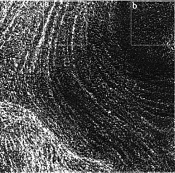
Fig. 1. Part of Jakobshavn Isbræ (North Ice Stream). Subset of ERS-lSAR dataset El-19930.1395.pn (transposed) from 8 May 1995. Subareas used for variogram analysis are indicated: (a) in center of ice stream showing curved flowlines (wl00.τ4.p2); and (b) in corner of subset without significant morphologic features (wl00.τ4.p4).

Fig. 2. Jakobshavn Isbm (subset of ERS-2 dataset E2-10958.2205.pn, georeferenced using Jakobshavn 1:250 000 maP(Kortog Matrikelstyrelsen, 1979). (a) MICROTOP 97 GRS survey area (areaS, area4, area5 of ground surveys with GRS during expedition MICROTOP 97). (b) Index of subset locations: MI, North Ice Stream; LCI, Lower Central Ice Stream; M, MICRO-TOP 97 GRS survey area.

For comparison with ground surveys, however, PRI-type data need to be georeferenced as precisely as possible, in particular since the areas of our ground surveys are relatively small (175 m × 75 m to 175 m × 200 m). The GEC product, which is georeferenced, was not available at the time of our analysis. As a cartographic base, the "Jakobshavn" 1:250 000 map sheet (Kort- og Matrikelstyrelsen, 1979) was used. The map was scanned, transformed to Universal Transverse Mercator coordinates and about 40 control points, identifiable both in the map and the SAR image, were used for georeferencing with the software package ENVI. Because points on the fast-moving ice surface cannot serve as control points, no control points close to the camp area on the inland ice are available. All control points are located on land and at easily identified locations such as promontories on lake shores or at the fjord coast. To minimize the error, all control points were selected at about the same elevation (as shown on the topographic map). After an initial pass, the 17 best control points were retained based on error analysis and knowledge of the geography of the area. The resulting accuracy is one pixel (= 12.5 m), the resolution of the scanned map was high enough to maintain a pixel size of 12.5 m after georeferencing. Image coordinates are counted from left to right (xaxis) and from top to bottom (j/ axis).

Absolute variogram values depend on the raster file format of the processed image (about 60 for sun^® raster files, about 1500–2000 for pgm files from a scale of 256 values). The absolute value of the variogram is not important in the analysis, and the selection of file type has technical reasons not relevant in this study.

We tested the effects of image-enhancement and resampling algorithms on variography for subset NI4 (see Fig. 2 for location; see Fig. 3 for results). As a default in ENVI, images of subareas are enhanced using histograms of subareas, this means a non-linear transformation effect on the spectrum and the variogram (Fig. 3a and b), and subareas cannot be compared any more. A linear transformation preserves the ratios and thus the comparability of subareas, the variogram structures are similar (except for a different scale factor for each transformed subset) (Fig. 3c and d). The following four figure panels (Fig. 3e-h) show variograms of the georeferenced and resampled dataset (the 100 × 100 pixel subset used in Fig. 3a–d, was georeferenced using the same control points as in the entire image). From 8 directional variograms the two that matched directions of Figure 3a–d were chosen. Resampling using cubic convolution (a weighted average, Fig. 3g and h) appears to retain features slightly better than nearest neighbour resampling (Fig. 3e and f), so cubic convolution was used in all following examples. Resampling hardly changes the minima and maxima in the variogram and thus the characterization parameters.

Fig. 3. Test of influence of image processing on variography. Test area on North Ice Stream (NI4), size 100 × 100 pixel, 1 pixel = 12.5m. ERS-2datasetE2-10958.2205.pn. Directional variograms (not filtered). Sub areas selected ni PRl-file: (a and b) image enhancement using histogram-based transformation, (a) 107° across flow, (b) 17° along flow (flow direction is southerly); (cand d) image enhancement using linear transformation, (c) 107° across flow, (d) 17° along flow; (ε andf) georeferenced using same control points as for georeferencing of entire image shown in Figure 2, and recalculation of grey values using nearest-neighbour averaging, with image enhancement using linear transformation, (e) 112.5° across flow, (f) 22.5° along flow; (gandh) georeferenced using same control points as for georeferencing of entire image shown in Figure 2, and recalculation of grey values using cubic convolution, with image enhancement using linear transformation, (g) 112.5° across flow, (h) 22.5° along flow.

5. Geostatistical Surface Characterization from 1995 Ers-1 and 1997 Ers-2 Sar Data, Jakobshavn Isbræ North Ice Stream

The principles of geostatistical surface characterization are demonstrated using examples from Jakobshavn Isbræ. The subset in Figure 1 contains a part of "North Ice Stream",where it flows around a rock promontory, changing from a southerly to westerly direction, before it joins the "South Ice Stream" about 8 km from the calving front. This is one of the most heavily crevassed areas, the crevasses group the seracs in flowline-parallel curved ridges. Thε pattern of the flowlines is clearly visible in the SAR image. Using the geo-statistical ice-surface classification system ICECLASS, directional variograms were calculated for 100 x100 pixel windows moving across a larger area. Suitability of different variogram types for derivation of characteristic parameters is demonstrated in Figure 4a–c. Comparison of the variogram (Equation (1)) with the residual variogram (Equation (2)) shows that there is no trend in the grey values of the investigated subset, so both variogram and residual variogram are equally suited. In Figure 4c, the residual variogram is smoothed using a Butterworth filter, this operation prevents an automated algorithm from catching on small wiggles in the variogram rather than correctly determining the characteristic minima and maxima. Filtering is particularly important when searching for longer-wavelength features. In Figure 4c and d two examples of variograms from different windows are shown to exemplify the structural differences between two surface types. Thε first example (wl00.τ4.p2) is located in the center of the ice stream and contains a section of thε curved flowlines (cf Fig. 1). Thε directional variograms reflect (1) the anisotropy of across-flow and along-flow variability, and (2) the regular hill-and-valley structure of the ridges of seracs, segmented by "valleys" of large crevasses. The across-flow spacing of ridges is 200 m (direction 2 is the direction of closest spacing), the significance of (2) is also captured in parameters p1 and p2, given in Table 1. Both parameters are highest for the across-flow direction and decrease to the along-flow direction, in which the minimum may not be distinguished. In contrast, the second example stems from the area in the inside of the curve of flow, located closer to the rock promontory. There are no significant features visible in the SAR data, and in fact, from field evidence, the area is crevassed but not regularly structured. Consequently, the resulting directional variograms do not exhibit significant minima. This exercise demonstrates that the two ice-surface provinces may be discriminated using geostatistical characterization based on SAR data.

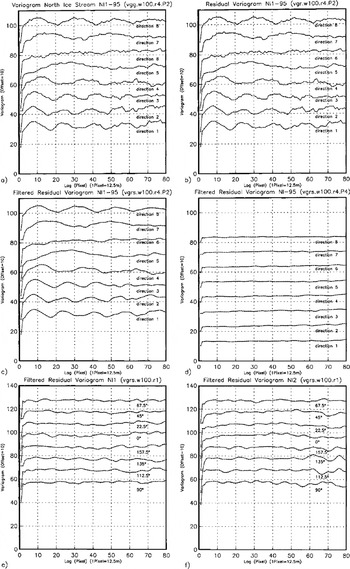
Fig. 4. Directional variograms from North Ice Stream. Eight directions, increasing from 0° (direction 1, × axis; × axis is approximately north, cf Kg 2) clockwise in steps of 22.5° to 157.5° (direction 8). (a–d) calculated from 1995 ERS-1 SAR dataset El-19930.1395.pn (transposed; ascending orbit) in 100×100pixel subareas shown in Figure 1. Residual variograms have been calculated and filtered (Butterworth filter). For ease of display, variograms are plotted with an offset of 10 per direction. In center of NI (Fig. 1a), surfacewithcurvedflowlines: (a) variogram of subarea wl00.r4.p2; (b) residual variogram ofSubareawl00.τ4.p2; ( c) Filtered residual variogram ofsubarea wl00.r4.P2 Near inside of bend of NI(Fig lb), without significant surface patterns: (d) filtered residual variogram of sub are a wl00.r4.p4. ( e) Filtered residual variogram of sub area Nil (Fig 2), same subarea as wl00.τ4.p2 in (a–c) on 1995 image, in center of NI, surface with curved flowlines; (f) filtered residual variogram of subarea NI2 (Fig 2), north of bend in NI. Both (e) and (f) calculated from 1997 ERS-2 SAR dataset E2-10958.2205pn (descending orbit, georeferenced (georeferencing with recalculation of grey values using cubic convolution) ) in 100 × 100 pixel subareas.

As a word of caution, it should be mentioned that the quality of the image of a given feature depends on the look-angle, and consequently differences between ascending mode and descending mode are significant. Thε 1995 ERS-1 image (Fig. 1) stems from an ascending orbit, the flow patterns are well-visible both in the image (Fig. 1) and in the variograms (Fig. 4a–c). In contrast, the same area barely shows flow patterns in the descending orbit 1997 image (Fig. 2, Nil) or characteristic maxima-minima sequences in the variogram (Fig. 4e). Both are much better discernable in a subset upstream of the corner where the flow is southerly (Fig. 2, NI2 and Fig. 4f). This example suggests that a combination of an ascending-mode and a descending-mode image may improve the classification results, but that requires accurate georeferencing.

6. Comparison of Variography from 1997 Ers-2 Sar Data with Contemporaneous Glacier-Roughness Surveys, Jakobshavn Isbræ Drainage Basin

One objective of expedition MICROTOP 97 to the inland ice was to collect high-resolution surface-roughness measurements, that may serve as ground truth for SAR data. The area of ground surveys is located in the Jakobshavn Isbræ drainage basin, close to, but just outside the heavily crevassed marginal area south of the South Ice Stream (Fig. 2). Threε areas with different surface characteristics were surveyed: (1) area3 is characterized by a complex morphology of large sastrugi, overprinted by melting processes, and with smaller structures in between; (2) area4 is dominated by large sastrugi; and (3) area5 is located in a blue-ice area, where the hill-and-valley pattern of the adjacent areas is partly drowned in daily melting and refreezing ice. Compared to other areas of the jakobshavn Isbræ drainage basin, all three areas have similar characteristics. Characteristic differences in variograms calculated from GRS data facilitate a classification of the types in areas area3, area 4, and area 5 (Reference Herzfeld, Mayer, Feller and MimlerHerzfeld and others, 2000).

Location of the survey areas was determined from GPS data of survey grid nodes (Reference Herzfeld, Mayer, Feller and MimlerHerzfeld and others, 2000), each of area 3, area 4, and area 5 was identified with a set of SAR pixels (cf. Fig. 2a) in the georeferenced image. Area3 is 336 pixel, area 4 345 pixel, and area 5 220 pixel in size. Variograms calculated for these areas are presented in Figure 5. Direction 67.5° corresponds most closely to the along-track direction of the GRS surveys (67°45’ geographical direction). For area 3 and area 4, 67.5° is also the direction of the closest minimum (parameter dirmin) in the variogram (Fig. 5), with spacing 5 pixel, mindist is also 5 pixel for 90° and 112.5°. This is an encouraging result, because the along-track direction in the ground surveys was selected normal to the strike of surface features (sastrugi and ridges, see Reference Herzfeld, Mayer, Feller and MimlerHerzfeld and others, 2000). The geometrical anisotropy is best observed in Figure 5b of area 4, this is also the area where the surface morphology is simplest. The spacing is 5 × 12.5 m = 62.5 m, this may correspond to groups of sastrugi. For area 5, the picture is similar, albeit not as clear, matching the observation that the surface in area 5 lies in the same general environment, but within a blue-ice area which partly drowns the ridge systems (Fig. 5c). Comparing Figure 5a–c it is apparent that an automated analysis at this scale would put all three areas in the same category. The analysis of GRS data facilitates a characterization of high-resolution surface structures not otherwise attainable.

Fig. 5. Directional variograms (unfiltered) of ERS-2 SAR datasetE2–10958.2205.pn contemporaneous to ground surveys during MICROTOP 97. Variograms calculated for GRS survey areas area3, area4, area5; located using GPS and georeferencing of ERS-2 data (recalculation of grey values using cubic convolution). Size of areas on SAR image matched with ground areas ( cf Fig. 2a). Eight directions as in Figure 4. For ease of display, variograms are plotted with an offset of 800 per direction: area3, 21×16= 336pixel; area4, 23 x15= 345pixel; area 5, 20 x11 = 220 pixel.

7. Comparison of Surface Characteristics of Three Areas on Jakobshavn Isbræ

Following the observation that area 3, area 4, and area 5 all lie in the same general environment of sastrugi and melting structures south of the margin of the ice stream, a larger area containing all ground-survey areas may be considered homogeneous, if compared to other types at the lower resolution of the SAR images. In this section, we investigate three areas (equal in size to the 40 x40 pixel envelope of the survey areas (Fig. 2)): (1) MICROTOP 97 GRS survey area (M2), dominated by sastrugi and melting structures: (2) an area on North Ice Stream (NI3), dominated by flowline-oriented crevasse patterns: (3) an area on lower "Central Ice Stream" (LCI2) near the calving front, dominated by irregularly oriented large crevasses and seracs (Fig. 2). Variograms for 8 directions are presented for each area in Figure 6, parameters are given in Table 2. We investigate the following criteria: total variance/sill value, isotropy spacing of characteristic features, regularity (of variogram) and significance parameter p2. To investigate the optimal window size for analysis, 100 × 100 pixel windows are studied (Fig. 7): Ml (MICROTOP 97 GRS survey area); NI2 (North Ice Stream); and LCI1 (Lower Central Ice Stream).

Fig. 6. Directional variograms (unfiltered) calculated for 40×40pixel-size areas from ERS-2 SAR dataset E2-10958.2205.pn (georeferenced, recalculation of grey values using cubic convolution) contemporaneous to MICROTOP 97 ground surveys. Eight directions as in Figure 4. For locations see Figure 2 (a) Area M2, containing MICROTOP 97 GRS survey areas area3, area4, area5 ( cf Fig. 2a); (b) area NI3;(c)areaLCI2.

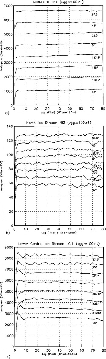
Fig. 7. Directional variograms (unfiltered) calculated for 100×100pixel-sized areas from ERS-2 SAR dataset E2–10958.2205.pn (georeferenced, recalculation of grey values using cubic convolution) contemporaneous to MICROTOP 97 ground surveys. Eight directions as in Figure 4. For locations see Figure 2 (a) Area Ml containing MICROTOP 97 GRS survey areas area3, area4,area5; (b) area NI2; (c) area LCIl.

8. Summary and Conclusions

This paper describes a first attempt to apply the geostatistical surface-characterization method to the analysis of SAR data from ERS-1 and ERS-2. The variogram is an ideal mathematical function to evaluate spatial data that lack absolute values, because it is calculated from increments of the data. Care needs to be taken to exploit the spatial resolution of the data optimally. The effects of image enhancement, common in satellite-image analysis tools and of grey-value resampling after georeferencing on variogram parameters were investigated. As a result, linear transformation in image enhancement and cubic convolution in resampling are now applied routinely.

Using geostatistical surface characterization, different ice-surface types may be distinguished. Examples are: a crevassed part of the ice stream where serac grouping and crevasse patterns follow the flow pattern of the ice on the North Ice Stream of Jakobshavn Isbræ; a heavily, but more chaotically, crevassed area near the calving front; and a crevasse-free area with a surface morphology of sastrugi, melting structures and blue-ice areas. Geometrical anisotropics, flow direction, and spacing of flowline-parallel surface features calculated from variogram parameters matched field observations on jakobshavn Isbræ. Such features on the heavily crevassed ice stream are on the order of 50–500 m. Smaller surface structures such as melting structures and sastrugi (meters to tens of meters), which typically dominate the morphology in crevasse-free areas may also be characterized using this approach, down to a resolution of 50 m. Glacier-roughness-sensor data provide high-resolution ground-truth data not otherwise attainable, that aid in the geostatistical characterization of ice-surface provinces from SAR data.

Consequently, the characteristic parameters derived in the characterization may be used in an automated geostatistical classification of ice surfaces from SAR data, applying a moving-window operator. For characterization of longwave structures from large windows (e.g. 100 × 100 pixel), best results are obtained if variograms are filtered prior to extraction of parameters for feature vectors. The optimal size of the moving window depends on the ice-surface morphological type; this problem is easily managed if individual areas need to be classified. In order to obtain a segmentation of a larger area into ice-surface provinces, a wedging of filters and windows of different sizes is necessary.