


1. Introduction
In mountainous regions, assessment of precipitation with high resolution and accuracy is of crucial importance for glacier mass-balance or hydrological studies. Due to the inhomogeneous precipitation distribution and sparse weather-station data, the assessment of precipitation remains challenging. Mountain areas modify large-scale circulation due to the orographic induced uplift of air masses generating orographic precipitation during saturated atmospheric conditions (e.g. Reference SmithSmith, 1979; Reference RoeRoe, 2005; Reference LinLin, 2007). The orography influences the formation of clouds and consequently the precipitation amount and spatial distribution between the windward and lee sides of the mountain range, creating sharp climate transitions. One of the sharpest climate transitions is found in Southern Patagonia (Reference Miller and SchwerdtfegerMiller, 1976; Reference Schneider, Glaser, Kilian, Santana, Butorovic and CasassaSchneider and others, 2003; Reference RoeRoe, 2005; Reference LinLin, 2007), where the prevailing westerlies of the Southern Hemisphere impinge on the perpendicular-running Southern Andes. This leads to a large-scale orographic lifting of air masses and the development of local-scale wind systems which are often accompanied by strong orographic precipitation events (Reference Miller and SchwerdtfegerMiller, 1976; Reference Paruelo, Beltrán, Jobbágy, Sala and GolluscioParuelo and others, 1998; Reference Schneider, Glaser, Kilian, Santana, Butorovic and CasassaSchneider and others, 2003). The local precipitation patterns depend on prevailing conditions, such as speed and direction of airflow, vertical stability, moisture content, geometry of the mountain range, and pre-existing atmospheric disturbances (e.g. extratropical cyclones) (Reference SmithSmith, 1979; Reference RoeRoe, 2005; Reference LinLin, 2007). Any change in the large-scale atmospheric circulation will cause changes in precipitation that differ widely between west-and east-facing sides of the Southern Andes. The resulting windward- and lee-side effects in spatial precipitation distribution and the high annual precipitation amounts further influence the mass balance of maritime glaciers such as Gran Campo Nevado (GCN) ice cap (Reference Schneider, Glaser, Kilian, Santana, Butorovic and CasassaSchneider and others, 2003, Reference Möller, Schneider and Kilian2007a), causing a high mass turnover and a short response time to changes in temperature and precipitation (Reference Möller, Schneider and KilianSchneider and others, 2007a; Reference Möller and SchneiderMöller and Schneider, 2008). For glaciological impact studies, climate datasets of global or regional climate models are often used to drive high-resolution glacier models. As a result of the coarse resolution of the topography, local-scale variations in orographic induced precipitation patterns in complex terrain are not resolved. To fill the spatial resolution gap between coarse- resolution data and the requirements for local glaciological impact studies, statistical downscaling methods based on station data such as local scaling factors or statistical transfer functions (Reference Reichert, Bengtsson and ÅkessonReichert and others, 1999; Reference Widmann, Bretherton and SalathéWidmann and others, 2003; Reference Radić and HockRadić and Hock, 2006) are often used. Precipitation is mostly distributed over complex terrain by using interpolation schemes, fixed vertical gradients (Reference OerlemansOerlemans, 1992; Reference HockHock, 2003; Reference SchulerSchuler and others, 2005) or altitude corrections (Reference Daly, Neilson and PhillipsDaly and others, 1994; Reference HutchinsonHutchinson, 1998; Reference Huss, Bauder, Funk and HockHuss and others, 2008). Since the availability and quality of station data in mountains is sparse and low, especially in snowy areas, the downscaling method for glaciological studies should be independent of station data to be applicable in mountainous regions without monitoring networks (Reference Schuler, Crochet, Hock, Jackson, Barstad and JohannessonSchuler and others, 2008; Reference Jarosch, Anslow and ClarkeJarosch and others, 2012). Besides statistical downscaling, high-resolution physical numerical models have been used for detailed estimation of precipitation at a spatial resolution of a few kilometers with promising results. However, their high computational requirements restrict their application to individual events. Therefore, this method is not yet suitable for long-term (multi-decadal to century) studies (Reference JiangJiang, 2003; Reference Medina, Smull and HouzeMedina and others, 2005; Reference Mölg and KaserMölg and Kaser, 2011).
In previous mass-balance studies at GCN, statistical precipitation downscaling methods based on station data have been applied (Reference Möller, Schneider and KilianMöller and others, 2007; Reference Möller, Schneider and KilianSchneider and others, 2007a; Reference Möller and SchneiderMöller and Schneider, 2008) and interpolated altitude-dependent by assuming a linear precipitation gradient (LPG). Because of the harsh weather conditions at GCN, the vulnerability of station measurement is high. A precipitation downscaling approach that does not require measured data is the preferred alternative. In addition, the strong influence of the orography on precipitation patterns at GCN is neglected by using a fixed gradient for precipitation distribution. A promising scheme for including this important effect is provided by applying orographic precipitation models (OPMs) to downscale precipitation in mountain areas.
To allow long-term applications at low cost, it is advisable to make a compromise between model complexity and model accuracy. OPMs have been developed and extended over recent decades, with variations in the degree of complexity (Reference SmithSmith, 1979; Reference AlpertAlpert, 1986; Reference Haiden, Kahlig, Kerschbaum and NobilisHaiden and others, 1990; Reference SinclairSinclair,1994; Reference Pandey, Cayan, Dettinger and GeorgakakosPandey and others, 2000; Reference Smith and BarstadSmith and Barstad, 2004; Reference Kunz and KottmeierKunz and Kottmeier, 2006a,Reference Kunz and Kottmeierb). Less complex upslope models estimate the condensation rate on the upslope region by means of the terrain-induced vertical air velocity and wind speed (Reference SmithSmith, 1979; Reference Neiman, Ralph, White, Kingsmill and PerssonNeiman and others, 2002) assuming that precipitation is only generated on the upslope regions (Reference SmithSmith, 1979; Reference SinclairSinclair, 1994). By including temporal delays of fallout rates and condensation, the upslope condensate is redistributed downstream without regard to terrain and evaporation of cloud water and hydrometeors on the lee side of mountain ranges (Reference Haiden, Kahlig, Kerschbaum and NobilisHaiden and others, 1990; Reference Hay and McCabeHay and McCabe, 1998; Reference SmithSmith, 2003). Recent studies further include three-dimensional airflow dynamics from linear theory in order to account for local terrain effects (Reference Jiang and SmithJiang and Smith, 2003; Reference Smith and BarstadSmith and Barstad, 2004; Reference Barstad and SmithBarstad and Smith, 2005; Reference Kunz and KottmeierKunz and Kottmeier, 2006a,Reference Kunz and Kottmeierb). Reference Smith and BarstadSmith and Barstad’s (2004) linear model of orographic precipitation has been validated in detail (Reference Barstad and SmithBarstad and Smith, 2005; Reference Smith and EvansSmith and Evans, 2007) and implemented successfully in hydrological (Reference Crochet, Jóhannesson and JónssonCrochet and others, 2007; Reference Caroletti and BarstadCaroletti and Barstad, 2010) and glaciological studies (Reference Schuler, Crochet, Hock, Jackson, Barstad and JohannessonSchuler and others, 2008; Reference Jarosch, Anslow and ClarkeJarosch and others, 2012). The main advantage of such an analytical model is the simplification of physical processes, which enables a longterm application for larger mountain ranges with high resolutions because of the low computational costs.
One main focus of this study is on the application of the OPM, which is based on Reference Smith and BarstadSmith and Barstad’s (2004) linear theory of orographic precipitation, to downscale precipitation for mass-balance studies at GCN with a horizontal resolution of 1 km. The OPM is driven by the US National Centers for Environmental Prediction and US National Center for Atmospheric Research (NCEP–NCAR) Reanalysis datasets of wind, temperature, relative humidity, geopotential heights, and precipitation, and implemented with a similar methodology to that described in Reference Schuler, Crochet, Hock, Jackson, Barstad and JohannessonSchuler and others (2008). Analysis of the sensitivity of mass-balance modeling of GCN to precipitation changes is another main focus of this study. Hence, two precipitation downscaling schemes (OPM and LPG) are used as the precipitation input of a simple mass-balance model. One aim is to assess the skill of the OPM at GCN, since the model provides a promising technique for downscaling precipitation in regions where the influence of orographic effects is high. A comparison of the OPM with a downscaling method used in earlier studies at GCN should provide details of the applicability, performance, advantages and disadvantages of the model. Ultimately, it would be desirable to achieve improved modeled results due to the application of the OPM, but sparse measured datasets might limit a complete validation.
After an introduction of the study site, a non-exhaustive overview of the methods is provided. Datasets and methodology are described in the following sections. We then validate the two precipitation downscaling methods with station and glaciological datasets. A discussion of the results concludes the paper.
2. Study Site
Most parts of the glaciated area in Patagonia can be found between 46° S and 51° S, where the Northern and Southern Patagonia Icefields with a total area of 17 200 km2 are located (Reference AniyaAniya, 1999). The high orographic induced precipitation amounts and the moderate summer temperatures at sea level cause a decrease of the snowline from 1400 m at the Northern and Southern Patagonia Icefields to ∼700 m near the Strait of Magellan, enabling the existence of smaller glaciated areas. One of these can be found in the study area in the south of the Mu͂noz Gamero peninsula at ∼53° S where the glaciated area extends to ∼252.56 km2, while GCN ice cap accounts for 199.5 km2 (Reference Möller, Schneider and KilianSchneider and others, 2007a). The largest area is made up by the plateau of GCN ice cap with the highest elevation of 1628 m a.s.l., which constitutes several individual outlet glaciers, some reaching sea level (Fig. 1) (Reference Schneider, Kilian and GlaserSchneider and others, 2007b). For the mass turnover of these outlet glaciers, calving into fjords or proglacial lakes plays an important role as reported for a series of Patagonian glaciers (Reference Warren and AniyaWarren and Aniya, 1999; Reference Porter and SantanaPorter and Santana, 2003). Furthermore, most glaciers are characterized by large ablation areas, comparatively small accumulation areas and high vertical mass-balance gradients. At some glaciers on the east side of GCN the accumulation and ablation areas are separated by steep steps, so that avalanches of ice and snow are the main mass transport mechanism. The high-level prevailing westerlies and the perpendicular-running Southern Andes between 48° S and 55° S cause harsh climate conditions at GCN including high wind speeds year-round and an outstanding precipitation gradient with windward and lee-side effects and estimated maximal precipitation amounts of ∼10000 mm a−1 at the glacier plateau of GCN (Reference Schneider, Glaser, Kilian, Santana, Butorovic and CasassaSchneider and others, 2003). It is reported that precipitation originating from westerly and northwesterly air masses accounts for up to 60% of all precipitation events (Reference Möller, Schneider and KilianSchneider and others, 2007a). The prevailing westerlies and the vicinity of the Pacific Ocean lead to a moderate mean annual temperature at sea level of 5.7°C (Reference Schneider, Glaser, Kilian, Santana, Butorovic and CasassaSchneider and others, 2003).

Fig. 1. Location of Gran Campo Nevado ice cap in Southern Patagonia. Profiles A and B are taken for the analysis of mass-balance gradients. Coordinates correspond to Universal Transverse Mercator (UTM) zone 18S.
The maritime climate conditions emphasize the sensitivity of GCN ice cap to climate change. According to Reference Möller and SchneiderMöller and Schneider (2008), glaciers are sensitive to temperature changes (−0.27 ± 0.001 m w.e. K−1), especially during the summer months. By contrast, a 10% shift in precipitation might lead to a mass-balance change of ∼+0.03 m w.e. Based on the climate conditions and the pronounced orographic precipitation effects, GCN provides an excellent study area to apply and evaluate an OPM.
3. Data
3.1. NCEP–NCAR Reanalysis data
The large-scale 6 hourly atmospheric data are derived from the NCEP–NCAR Reanalysis data provided on a 2.5° × 2.5° grid (Reference KalnayKalnay and others, 1996). The selected gridpoint is centered at 52.5° S, 72.5° W. The following variables are used: horizontal (U) and vertical (V) wind components, temperature (T), relative humidity (rH), geopotential heights (hgt) and precipitation (P). The environmental and moist adiabatic lapse rate are calculated using datasets of air temperatures from the 925 and 500 hPa levels. The wind components of the 500 hPa level are used for the OPM application, since they are most suitable to simulate the large-scale prevailing wind conditions in Southern Patagonia. The datasets of precipitation and relative humidity (925 hPa) are needed to calculate the background precipitation and to determine days with orographic precipitation.
3.2. Meteorological and glaciological data
The application and validation of the OPM and LPG is limited to April 2010–July 2011 owing to the availability of measured precipitation data. During this period, the daily precipitation data of two automatic weather stations (AWSs) at different altitudes and distance to GCN ice cap are used for validation. AWS Paso Galería is located at the northeastern pass of GCN at 383 m a.s.l., while AWS Puerto Bahamondes is located ∼3.5 km east of the ice margin at 26 m a.s.l. (Fig. 1; Reference Schneider, Glaser, Kilian, Santana, Butorovic and CasassaSchneider and others, 2003). All data except precipitation are measured 2 m above the surface. Precipitation is measured at a height of 1 m using an unshielded tipping-bucket rain gauge. This type of precipitation measurement is reliable, but large uncertainties may occur during intensive precipitation events, high wind speeds and snowfall. In the years 2000–09 the shaking of the tipping buckets caused wind-induced errors. To minimize these errors, the rain gauges have been additionally fixed since 2010, which limits the time period of validation (Fig. 2). According to Reference Schneider, Glaser, Kilian, Santana, Butorovic and CasassaSchneider and others (2003), the precision of the tipping-bucket rain gauge at Puerto Bahamondes is estimated to be ±20%. More substantial negative deviations of precipitation during the winter months might occur in the case of snowfall, since a heating system is not included. The daily air temperature data of Puerto Bahamondes are needed to interpolate temperature for GCN for mass-balance modeling. Additionally, ablation stake measurements on Glaciar Lengua (Fig. 1) are available for the period 2000–05, which enable the evaluation of the two precipitation downscaling methods by estimating the impact on mass balance by a degree-day model (DDM).

Fig. 2. Precipitation measurement periods at AWS Paso Galería and AWS Puerto Bahamondes.
The uncertainty of ablation stake measurements has been estimated to be about ±9% according to ablation measurements during the 2000 austral summer by Reference SchneiderSchneider (2003). This estimate refers to the period and stake number Set2000 (see Table 2). Differences in ablation between single stakes at the same altitude might occur due to measurement inaccuracies, stake movement within the borehole or due to the small-scale spatial variability of the roughness of the glacier surface. However, these uncertainties can be reduced by taking mean values over all ablation stake measurements at the same altitude (Set2000, L1–L3, L1–L5, L2–L4, B1–B3; Table 2). A more detailed description of the ablation measurement network is provided by Reference SchneiderSchneider (2003) and Reference Möller, Schneider and KilianSchneider and others (2007a).
Table 2. Validation of mass-balance modeling with ablation stake measurements at Glaciar Lengua. Date format is dd.mm.yyyy

4. Methods
4.1. Model description of orographic precipitation
The OPM of Reference Smith and BarstadSmith and Barstad (2004) is an extension of an earlier version of a simple upslope model (Reference SmithSmith, 1979) and upslope-advection model (UAM; Reference SmithSmith, 2003). The models estimate precipitation resulting from forced orographic uplift of air masses over a mountain assuming stable and saturated atmospheric conditions. The simple upslope model created by Reference SmithSmith (1979) estimates the condensation rate on the upslope region by the terrain-induced vertical air velocity, the horizontal wind speed, and assuming direct fallout of condensed water. The terrain-induced vertical air velocity penetrates upwards through the moist layer without considering decay or oscillation with altitude.
Since the original model does not account for lee-side transport, it underestimates orographic precipitation in these regions. Reference SmithSmith (2003) developed a UAM on the basis of this upslope model, including the advection of water vapor described by timescales for conversion τc , and fallout τ f of hydrometeors. Reference Smith and BarstadSmith and Barstad (2004) extended the UAM by designing a linear orographic precipitation model which also considers airflow dynamic and downslope evaporation.
The OPM consists of a pair of steady-state advection equations for atmospheric water, describing the vertically integrated advection of cloud water and hydrometeors:
The left terms describe the steady-state advection of vertically integrated condensed cloud water q
c(x, y) and the hydrometeor density q
s(x,y) with the horizontal wind U. The last term of Eqn (1) describes the conversion of cloud water to hydrometeors. The empirical timescale τc
determines the time required for conversion. This term then serves as the source term for Eqn (2) which describes the change of hydrometeor density. The final fallout rate of hydrometeors is given by the last term ![]() of Eqn (2) (Reference Smith and BarstadSmith and Barstad, 2004).
of Eqn (2) (Reference Smith and BarstadSmith and Barstad, 2004).
The amount of precipitation is controlled by the delay parameters of conversion and fallout of condensed water.
According to Reference SmithSmith (2003), a Fourier transform (FT) of the orographic precipitation formulations is applied for an easier solution and to allow any wind direction to be used without rotating the coordinate system. To reduce the computational time of the OPM the fast Fourier transform (FFT) is used and in the following labeled by (^) (Reference SmithSmith, 2003).
The general solution for orographic precipitation for each Fourier component (k, l) can be obtained by combining Eqns (1) and (2):

In most studies τ
f and τc
are assumed to be equal. Since tuning of these constants by means of station data is not recommended (Reference Smith and BarstadSmith and Barstad, 2004), both timescales are derived from atmospheric data. According to Reference Jiang and SmithJiang and Smith (2003), τ
f can be calculated by ![]() , where H
b is the cloud-base height and V the mass-weighted average falling speed, which is suggested to vary between 1 and 2 m s−1. τc
and τ
f are set equal.
, where H
b is the cloud-base height and V the mass-weighted average falling speed, which is suggested to vary between 1 and 2 m s−1. τc
and τ
f are set equal.
A further improvement on earlier versions of the OPM is in the representation of airflow dynamics effects. The source term ![]() is given by
is given by
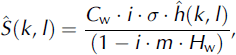
including an uplift sensitivity factor C
w, the water vapor scale height H
w, the complex number i, the intrinsic frequency σ, the orography ![]() , and the vertical wave number m. The thermodynamic uplift sensitivity factor
, and the vertical wave number m. The thermodynamic uplift sensitivity factor ![]() incorporates the effect of saturation water vapor density ρ
s, the moist adiabatic lapse rate Γ
m and the environmental lapse rate γ. The water vapor depth
incorporates the effect of saturation water vapor density ρ
s, the moist adiabatic lapse rate Γ
m and the environmental lapse rate γ. The water vapor depth ![]() is defined by the gas constant of vapor R
v, the latent heat L, the environmental temperature T
ref and lapse rate γ. The intrinsic frequency σ = U · K + V · l takes into account the airflow dynamics. The variation of vertical velocity with altitude is implicated using linear Boussinesq mountain wave theory. One of the airflow features is the decay of vertical velocity with altitude, which also leads to a reduction of condensation of water vapor to the lateral airflow around mountains reducing the vertical displacement of the air parcels (Reference Crochet, Jóhannesson and JónssonCrochet and others, 2007). The airflow over mountains may be modified due to condensation and evaporation during ascent and descent of the saturated air masses. Moisture in air masses influences the static stability which in turn weakens the gravity wave amplitude (Reference JiangJiang, 2003; Reference Kunz and WassermannKunz and Wassermann, 2011). The calculation of the vertical wavenumber therefore contains the buoyancy frequency in a saturated atmosphere, the moist Brunt–Väisälä frequency N
m:
is defined by the gas constant of vapor R
v, the latent heat L, the environmental temperature T
ref and lapse rate γ. The intrinsic frequency σ = U · K + V · l takes into account the airflow dynamics. The variation of vertical velocity with altitude is implicated using linear Boussinesq mountain wave theory. One of the airflow features is the decay of vertical velocity with altitude, which also leads to a reduction of condensation of water vapor to the lateral airflow around mountains reducing the vertical displacement of the air parcels (Reference Crochet, Jóhannesson and JónssonCrochet and others, 2007). The airflow over mountains may be modified due to condensation and evaporation during ascent and descent of the saturated air masses. Moisture in air masses influences the static stability which in turn weakens the gravity wave amplitude (Reference JiangJiang, 2003; Reference Kunz and WassermannKunz and Wassermann, 2011). The calculation of the vertical wavenumber therefore contains the buoyancy frequency in a saturated atmosphere, the moist Brunt–Väisälä frequency N
m:

Several different calculations of N m are discussed in detail by Reference Durran and KlempDurran and Klemp (1982). In this study, Reference Smith and BarstadSmith and Barstad’s (2004) formulation is applied:
Here g = 9.81 m s−2 is the mean gravitational acceleration of the Earth, and γ and Γ m are the actual temperature lapse rate and the moist adiabatic lapse rate, respectively.
The FFT enables a simple multiplication effect of the airflow dynamics and cloud time delay parameters solving the linear model more easily. Combining Eqns (3) and (4) gives

The final term of orographic precipitation distribution is obtained by an inverse Fourier transformation.
where P∞ represents the background precipitation. The precipitation generation is shifted downstream of the water source region and depends on the wind speed and the cloud time parameter (τc , τ f). The simple representation of the major physical processes of orographic precipitation, the fast implementation and short computational time are the main advantages of the OPM. Nevertheless, the OPM is limited to stable and saturated air masses, not capturing flow blocking effects nor being applicable during unstable atmospheric conditions.
4.2. Linear precipitation downscaling
A common method for obtaining spatial precipitation fields as input for mass-balance studies is based on a linear increase in precipitation with altitude (Reference OerlemansOerlemans, 1992; Reference Braithwaite and ZhangBraithwaite and Zhang, 2000; Reference HockHock, 2003; Reference SchulerSchuler and others, 2005; Reference Möller, Schneider and KilianMöller and others, 2007; Reference Buttstädt, Möller, Iturraspe and SchneiderButtstädt and others, 2009). In earlier mass-balance studies at GCN, a linear precipitation gradient of 5% (100 m)−1 was applied, assuming that the precipitation amount rises from ∼6500 mm a−1 to ∼10000 mm a−1 between sea level and GCN plateau (Reference Schneider, Glaser, Kilian, Santana, Butorovic and CasassaSchneider and others, 2003). This assumption is partially based on measured precipitation data (e.g. AWS Puerto Bahamondes) during the period 1999–2002. However, the data contain measurement errors caused by high wind speeds, which could not be reduced until 2010 (Section 3.2). The annual precipitation amount at Puerto Bahamondes for the period April 2010–March 2011 is 3950 mm a−1, which is significantly lower than the mean annual precipitation amount of 6500 mm a−1 (1999–2002), used by Reference Schneider, Glaser, Kilian, Santana, Butorovic and CasassaSchneider and others (2003). The annual precipitation at Paso Galería amounts to 6160 mm a−1 (April 2010–March 2011) (Fig. 1). Using the measured precipitation data of both available AWSs between 2010 and 2011 yields a precipitation gradient of ∼15% (100 m)−1 which is used in this study. Precipitation is downscaled from NCEP–NCAR data to AWS Puerto Bahamondes by using quantile mapping (Reference Panofsky and BrierPanofsky and Brier, 1968; Wilby, 1997; Reference Hay and ClarkHay and Clark, 2003) and then interpolated linearly with altitude.
4.3. Degree-day model
The mass balance at GCN is calculated by applying a DDM. The DDM has been presented in several studies (Reference BraithwaiteBraithwaite, 1981; Reference HockHock, 2003; Reference SchulerSchuler and others, 2005; Reference Radić and HockRadić and Hock, 2006; Reference Buttstädt, Möller, Iturraspe and SchneiderButtstädt and others, 2009). Since it has already been applied for mass-balance studies at GCN, we applied the identical DDM, using the same meteorological input parameters, and boundary conditions as described by Reference Möller, Schneider and KilianMöller and others (2007) and Reference Möller and SchneiderMöller and Schneider (2008). The precipitation gradient has been corrected as described earlier. The accumulation A and ablation M are calculated for specific altitudes a of the glacier surface. Total accumulation results from the sum of daily solid precipitation SP
a
,
i
. Melting rates are assumed to be proportional to the positive mean daily air temperature Ta
,
i
. The following approach usually contains a stochastic term with ![]() :
:
The sensitivity of ablation to temperature depends on the degree-day factors (DDFs) which are set to 8.6 mm K−1 d−1 and 4.3 mm K−1 d−1 in the cases of (f ice) and snow surface (f snow), respectively. The f ice is based on ablation stake measurements carried out on the outlet glacier Glaciar Lengua in 2000 (Reference Schneider, Kilian and GlaserSchneider and others, 2007b). Excluding the highest outlier, the median of f ice is 8.6 mm K−1 d−1. The f snow has been set to 50% of f ice, as widely assumed (Reference BraithwaiteBraithwaite, 1981; Reference HockHock, 2003; Reference Radić and HockRadić and Hock, 2006; Reference Möller, Schneider and KilianMöller and others, 2007; Reference Buttstädt, Möller, Iturraspe and SchneiderButtstädt and others, 2009). The specific mass balance is obtained by subtracting ablation and accumulation.
The DDM is initialized by the characteristic snow-cover pattern remaining from the last accumulation period. The snow thickness is estimated to increase linearly between 300 and 700 m a.s.l. from 0 to 500 mm. A sensitivity analysis of various snow-cover start conditions on the mass balance has been carried out by Reference Möller, Schneider and KilianMöller and others (2007) and they are estimated to change the mass balance by ±15 mm a−1.
The DDM is forced by using daily temperatures with a linearly decreasing temperature lapse rate of T inc = −0.58°C (100 m)−1 based on air temperature measurements at GCN (Section 3.2) and daily solid precipitation. According to Reference Möller, Schneider and KilianMöller and others (2007), the transition from liquid to solid precipitation SP a , i depends on the air temperature as follows:
Hence, the proportion of daily solid precipitation SPP a ,i for specific altitudes is smoothly scaled between 100% and 0% within the temperature range 0−2°C.
5. Data Processing and Filtering
Both precipitation downscaling methods (OPM and LPG) have been applied for the time period April 2010–July 2011. The same period is used to calibrate and validate the methods by means of station data. The methodology is illustrated in Figure 3.

Fig. 3. Flow chart of the applied methodology. U, V, T, rH, hgt, P are meteorological variables as described in the text.
The OPM replaces the orographic part of the NCEP– NCAR precipitation data by a high-resolution orographic precipitation field. In a first step, the large-scale background precipitation is determined by subtracting the orographic fraction from the NCEP–NCAR precipitation data. For this purpose the OPM is forced by NCEP–NCAR’s coarse digital elevation model and 6 hourly atmospheric data. The subtracted coarse-grid orographic part is then replaced by a high-resolution orographic precipitation field which is obtained by applying the OPM to the high-resolution Shuttle Radar Topography Mission data and the same atmospheric conditions (Reference JóhannessonJóhannesson and others, 2007; Reference Schuler, Crochet, Hock, Jackson, Barstad and JohannessonSchuler and others, 2008; Reference Jarosch, Anslow and ClarkeJarosch and others, 2012).
Since the OPM is constrained by saturated and stable atmospheric conditions, days that do not fulfill these constraints have been filtered out. According to these constraints, orographic precipitation is only possible if the air is almost saturated (>90%) and the atmosphere is stably stratified ![]() (Reference Smith and BarstadSmith and Barstad, 2004). Only if these constraints are satisfied is the high-resolution orographic part added, otherwise only the coarse-grid background precipitation is used.
(Reference Smith and BarstadSmith and Barstad, 2004). Only if these constraints are satisfied is the high-resolution orographic part added, otherwise only the coarse-grid background precipitation is used.
The second method (LPG) downscales the daily NCEP–NCAR precipitation to station data (AWS Puerto Bahamondes) using quantile mapping. The downscaled precipitation at this station is then extrapolated with a linear gradient of 15% (100 m)−1 to obtain daily precipitation fields for the entire ice cap (Section 4.2).
This methodology enables precipitation for mass-balance studies to be downscaled for the period 2000–05, when no reliable measured precipitation data are available. A further interpolation of the precipitation fields of both downscaling methods to 90 m is required in order to implement the daily precipitation fields into the DDM.
6. Results
6.1. Calibration time period
Before the two methods are compared in detail, the reliability of the derived OPM parameters is reviewed. The calculated parameters H
w, N
m, C
w and τ
f describing the atmospheric conditions in 2010–11 are in good agreement with the idealized values of Reference Smith and BarstadSmith and Barstad (2004). The depth of the water vapor varies between 1790 and 3988 m, with a mean value of 2480 m. The Brunt–Väisälä frequency ![]() yields only positive values, which fulfills the stability constraint of the OPM. The frequency varies between 0.007 s−1 and 0.01 s−1 depending on the environmental lapse rate and the water vapor in the atmosphere. The atmospheric conditions are permanently stable. The second constraint of the model considering the saturation of the atmosphere (>90%) is fulfilled on 66% of the days.
yields only positive values, which fulfills the stability constraint of the OPM. The frequency varies between 0.007 s−1 and 0.01 s−1 depending on the environmental lapse rate and the water vapor in the atmosphere. The atmospheric conditions are permanently stable. The second constraint of the model considering the saturation of the atmosphere (>90%) is fulfilled on 66% of the days.
According to Reference Smith and BarstadSmith and Barstad (2004), C w should range between 0.001 and 0.02, which corresponds with the range of values calculated (0.004–0.014). The mean time of hydrometeor fallout τ f is 2145 s, with a standard deviation of 237 s. These values are higher than those reported by Reference Crochet, Jóhannesson and JónssonCrochet and others (2007), Reference Schuler, Crochet, Hock, Jackson, Barstad and JohannessonSchuler and others (2008) and Reference Kunz and WassermannKunz and Wassermann (2011), and the idealized values of Reference Smith and BarstadSmith and Barstad (2004). This indicates a longer conversion time and delayed fallout of rain or snow. Consequently, this reduces the maximal modeled precipitation amount, and therefore smooths daily extreme precipitation events. Higher τ f values might be a result of the parameterization of the mass-weighted average falling speed which was set to 1.3 m s−1. Together with the high wind speeds at the 500 hPa level, this leads to realistic simulations of monthly precipitation amounts at the AWSs and the spatial distribution over GCN. Comparing the precipitation amount over the entire application period (April 2010–July 2011) between the two methods, significant differences are obtained in the maximal amount and in the spatial distribution (Figs 4 and 5). The maximal precipitation amount of ∼18000 mm (∼13 500 mm a−1) produced by LPG is higher than the amount of the OPM with ∼13 600 mm (∼10 200 mm a−1). Since the LPG interpolates precipitation with altitude, the location of the precipitation maximum is found at the highest point of the GCN. The OPM, however, shows a pronounced shift towards the lee side. The position of the daily maximal amount of the OPM depends on the daily atmospheric conditions.

Fig. 4. Precipitation spatial distribution for the period April 2010– July 2011 based on the LPG. The location of Paso Galería and Puerto Bahamondes is marked by red dots. Coordinates correspond to UTM zone 18S.

Fig. 5. Precipitation spatial distribution for the period April 2010– July 2011 based on the OPM. The location of Paso Galería and Puerto Bahamondes is marked by red dots. Coordinates correspond to UTM zone 18S.
Total precipitation amounts are overestimated at both AWSs, with deviations ranging from +2.0% to +2.6% by the LPG. The OPM overestimates the precipitation amount at Paso Galería by 1.5% and underestimates it at Puerto Bahamondes by 1.8% (Table 1). The deviations of both methods are within the accuracy of the precipitation measurement of ±20% (Section 3.2).
Table 1. Observed and modeled precipitation amounts of the OPM and the LPG (in parentheses), the relative precipitation differences, and the monthly correlations between observed and modeled data for AWS Paso Galería and AWS Puerto Bahamondes

Differences in precipitation amounts are larger on a monthly scale (Fig. 6). The OPM underestimates the monthly amount during austral summer at Paso Galería, where monthly precipitation amounts of up to 1100 mm occur.

Fig. 6. Modeled versus observed monthly precipitation amounts at Paso Galería and Puerto Bahamondes based on LPG and OPM.
This might be for different reasons. First, hydrometeors are advected far downstream and spread out due to high τ values, hence reducing the maximal precipitation amount. Second, the reanalyzed data show no pronounced annual seasonal cycle in relative humidity and precipitation, which affects the OPM results. During austral winter, precipitation is generally overestimated for Paso Galería by the OPM, which might be partially explained by the underestimation of measured precipitation in the case of snowfall, due to unheated tipping buckets. By contrast, deviations are smaller by the LPG, since the method itself includes the measurement errors. Taking all this into account leads to a weaker seasonality in modeled precipitation by the OPM compared to the LPG and therefore to slightly higher deviations between modeled and observed precipitation in the winter and summer months. Nevertheless, the daily root-meansquare errors (RMSE) between OPM and observed data for Paso Galería and Puerto Bahamondes are 16.0 and 10.6 mm, respectively. The RMSE are smaller than the RMSE of the differences between LPG and observed data for Paso Galería (17.5) and Puerto Bahamondes (11.4), but compared to the measurement error these differences give no further evidence of better performance. The correlation of monthly precipitation sums is higher between OPM and observed data at Puerto Bahamondes, even though the precipitation amounts of LPG are downscaled on the basis of Puerto Bahamondes (Table 1).
6.2. Sensitivity of mass-balance modeling 2000–05
The modeled mean annual mass balances show distinct spatial patterns as a result of the large differences of the precipitation fields. As illustrated in Figure 7, the highest differences in mean annual mass balance occur on the summit of the ice cap. The larger accumulation amounts produced by the LPG cause high positive differences of up to +3.0 m w.e. in annual mass balance solely on the summit. Daily air temperature at the summit of GCN is mostly below 0°C, hence almost all precipitation is accumulated as solid precipitation. Negative differences of up to −1.32 m w.e. a−1 along the outlet glaciers and steep faces of GCN are caused by higher melt rates by the LPG (Fig. 7). Daily melt rates at the lower altitudes of GCN depend on the snow-cover distribution because of the positive albedo feedback. The snow-cover distribution, however, is determined by the precipitation fields derived from both methods. Hence, the implementation of different DDFs for snow and ice surfaces leads to a variation of ablation rates between OPM and LPG.

Fig. 7. Spatial differences in modeled mean annual mass balance of GCN for the period 2000–05 by subtracting OPM from LPG. Coordinates correspond to UTM zone 18S.
Observed and modeled ablation are listed in Table 2. The results of the modeled ablation rates of both methods are mostly within the range of measurement uncertainties. Taking the mean values of ablation at L1–L3, L1–L5, L2–L4 and B1–B3 for each period reduces the measurement uncertainty, which might be one reason for the small deviations between observed and modeled ablation for both methods. The modeled ablation rates at stake LAWS for both available periods and methods are in good agreement with observed ablation. In the period 2004/05, larger differences occur at the ablation stakes Lup in the case of the LPG, and Lup–up for both methods. The latter might be due to large measurement uncertainties. Besides measurement inaccuracies, further uncertainties in model output are given by the need of the DDM.
The correlations between measured and modeled ablation for OPM and LPG are similar, with r 2 = 0.86. Similar modeled ablation rates were expected, since the differences in modeled mass balance at the altitudes of ablation stake measurements (428–504 m a.s.l.) are low due to the small annual amount of solid precipitation (Fig. 7). The validation using ablation data therefore showed no pronounced differences between the two approaches. Since the ablation data are sparse and restricted to a narrow elevation band, no further qualitative and quantitative assessment of mass-balance distribution can be carried out.
The impact of the two methods on mass-balance calculations differs and consequently influences the estimation of the equilibrium-line altitude (ELA). This can be illustrated by comparing modeled mass-balance gradients for two outlet glaciers, Glaciar Oeste South (A) and Glaciar Galería (B) (Figs 8 and 9). The mass-balance gradients are calculated along the profile lines shown in Figure 1. The mass-balance gradient of the LPG is greater on the windward as well as on the lee side. The estimated ELA on the windward side is located at 940 m for both methods. On the lee side the ELA remains the same for LPG, but is modeled to be at 890 m in the case of the OPM. A shift of the modeled ELA of −50 m would lead to a pronounced change in the modeled ice dynamic of Glaciar Galería. The choice of the precipitation downscaling method could lead to pronounced differences in modeled glacier dynamics. The spatial variations in mass balance and ice dynamics between windward and lee-side glaciers are assumed to be of crucial importance for GCN ice cap. Orographic effects could be considered by applying the OPM. Due to the insufficient ablation data we cannot prove that either method is superior.

Fig. 8. Modeled mass-balance gradients between OPM and LPG along profile A on Glaciar Oeste (Fig. 1).

Fig. 9. Modeled mass-balance gradients between OPM and LPG along profile B on Glaciar Galería (Fig. 1).
7. Summary and Conclusion
Two conceptual precipitation downscaling methods have been applied to GCN ice cap to analyze the impact on mass-balance modeling. An orographic precipitation model, driven by large-scale atmospheric variables taken from NCEP–NCAR datasets, has been applied to downscale 6 hourly precipitation fields with a resolution of 1 km for GCN. This method has been compared to a second downscaling approach where precipitation was downscaled to station data using quantile mapping and further interpolated linearly with altitude. The applications of both precipitation downscaling methods are in good agreement with station data. The LPG represents the precipitation distribution and amount between sea level and ∼400 m a.s.l. well, but at higher altitudes the annual precipitation amount is much higher than in the OPM-based method. It is also questionable if one can assume only one linear increase for both the windward and lee side of GCN. Due to the high wind speeds and the strong influence of orographic effects, a possible shift of the maximal annual precipitation amount towards the lee side is assumed. GCN ice cap is well suited to the application of the OPM because of its location within the westerlies. Since the OPM is initialized by coarse-resolution reanalyzed data, local differences in atmospheric conditions are not included. The missing seasonality of the NCEP–NCAR data affects the OPM results. The implementation of both downscaling approaches into mass-balance modeling illustrates the high sensitivity of accumulation patterns. Both the location of the ELA and the mass-balance gradient depend on the downscaling method. Such changes might influence the ice dynamic.
In general, a successful application of the OPM has been achieved. A significant improvement of the modeled precipitation fields due to the OPM was expected, but the validation of both approaches by means of observed data did not show a significant difference in the performances.
The sparse data of weather-station and ablation-stake measurements have limited the validation to the lower altitudes of GCN where the modeled results of both methods differ only slightly. Therefore, both approaches seem to be applicable to downscale precipitation at GCN.
At GCN plateau the modeled results showed larger differences in the maximal precipitation amount and distribution, but cannot be evaluated using measured data at this stage.
The daily precipitation fields and the maximal precipitation amounts in the summit region modeled by the OPM seem to be more realistic, but have to be further validated based on a larger number of measured datasets. The main focus of future projects at GCN, therefore, will be on an expansion of the current weather-station network including the summit region and the ablation measurements. This will further improve understanding of the spatial precipitation distribution and the influence of orographic precipitation effects on the mass-balance distribution at GCN.
Acknowledgements
We thank all members of the various field campaigns in recent years, in particular Rolf Kilian, Michael Glaser and Marco Möller, for their efforts in obtaining mass-balance and weather data from GCN.


