


Introduction
Silverleaf nightshade (Solanum elaeagnifolium, Cav.) is a highly invasive weed that has spread rapidly worldwide, infesting both irrigated and rainfed agricultural systems (Karmezi et al. Reference Karmezi, Krigas and Argyropoulou2022; Krigas et al. Reference Krigas, Votsi, Samartza, Katsoulis and Tsiafouli2023). Native to the southwestern United States and northern Mexico, S. elaeagnifolium has been introduced into numerous countries, including Greece, Morocco, India, Tunisia, Egypt, and Australia, primarily due to human activities (Roberts and Florentine Reference Roberts and Florentine2022; Sayari et al. Reference Sayari, Brundu, Soilhi and Mekki2022; Uludag et al. Reference Uludag, Gbehounou, Kashefi, Bouhache, Bon, Bell and Lagopodi2016). It is a deep-rooted perennial plant that reproduces sexually through seed production and asexually via rhizomes, enabling rapid colonization (Tataridas et al. Reference Tataridas, Jabran, Kanatas, Oliveira, Freitas and Travlos2022a). The weed is thus very adaptable and thrives in diverse environments, such as natural reserves, riverbanks, and cultivated fields (Chavana et al. Reference Chavana, Singh, Vazquez, Christoffersen, Racelis and Kariyat2021; Mekki Reference Mekki2007). Introduced into Israel in the 1950s, S. elaeagnifolium has become a significant weed pest, especially in irrigated summer crops such as cotton (Gossypium hirsutum L.), watermelon [Citrullus lanatus (Thunb.) Matsum. & Nikai], sorghum [Sorghum bicolor (L.) Moench], and maize (Zea mays L.), as well as in orchards.
The management of S. elaeagnifolium in Israel is a complex and challenging task, mainly due to the limitations of current herbicides: the registered herbicides that are selective and are recommended for S. elaeagnifolium, such as aminopyralid and imazapyr, are not suitable for agricultural crops (Wu et al. Reference Wu, Stanton and Lemerle2016), and other herbicides that are efficacious, such as glyphosate and glufosinate ammonium, lack selectivity and are therefore suitable for use only in limited control scenarios, such as preplanting preparation (Gitsopoulos et al. Reference Gitsopoulos, Damalas and Georgoulas2017). Furthermore, the use of mechanical control methods, including cultivation and mowing, for managing S. elaeagnifolium is problematic due to the extensive root network of this weed: the soil disturbance caused by mechanical control methods can result in the breakage of the weed rhizomes, thereby promoting an increase in the spread and density of propagules, both of which facilitate colonization of new areas (Stanton et al. Reference Stanton, Wu and Lemerle2011; Tataridas et al. Reference Tataridas, Kanatas and Travlos2022b; Wu et al. Reference Wu, Stanton and Lemerle2016). To effectively manage this weed, it is necessary to elaborate and adopt new methods that require expanded knowledge of its biology and ecology (Chauhan Reference Chauhan2022; Westwood et al. Reference Westwood, Charudattan, Duke, Fennimore, Marrone, Slaughter, Swanton and Zollinger2018); such methods can then be integrated into management strategies based on optimal herbicide and mechanical control applications (Grundy et al. Reference Grundy, Mead and Burston2003; Krueger-Mangold et al. Reference Krueger-Mangold, Sheley and Svejcar2006).
The rhizomes of S. elaeagnifolium are the main dispersal organ of this perennial species. However, the literature on the biological and environmental factors that impact the sprouting, establishment, and development of S. elaeagnifolium rhizomes is limited, with the available literature focused mainly on the impact of rhizome fragment length on plant establishment. Among those studies is a greenhouse study that assessed shoot, dry mass, and fruit production of S. elaeagnifolium plants that were developed from rhizomes with various fragment lengths. This study found that 20-cm fragments gave rise to taller plants compared with those originating from 5-cm and 10-cm fragments (Boyd and Murray Reference Boyd and Murray1982). However, this study did not evaluate the impact of fragment length on the sprouting pattern of the weed or the interaction of this biological parameter with environmental factors.
Among the various environmental factors influencing the sprouting dynamics and early establishment of weeds, temperature is one of the most prominent (Cezar Moraes de Aguiar et al. Reference Cezar Moraes de Aguiar, Ferreira Mendes, Heringer Barcellos Júnior, Gomes da Silva, Barbosa Xavier da Silva, Alberto da Silva and Ferreira Mendes2022; Peters et al. Reference Peters, Breitsameter and Gerowitt2014). Consequently, several studies have concentrated on creating prediction models based on thermal time (TT), specifically growing degree days (GDD). The importance of these models, which quantify accumulated heat units above a minimal threshold, lies in their ability to forecast crucial developmental stages, such as rhizome sprouting, for particular species (Dorado et al. Reference Dorado, Sousa, Calha, González-Andújar and Fernández-Quintanilla2009; Loddo et al. Reference Loddo, Masin, Otto and Zanin2012). Thus, these thermal models enable a more precise understanding of the effects of temperature on plant growth, development, and sprouting dynamics, thereby facilitating the formulation of targeted management strategies to effectively mitigate the spread and impact of these species. However, the construction of a predictive model necessitates preliminary studies to obtain species-specific biological parameters, such as base (T b), optimal (T o), and ceiling (T c) temperatures, also referred to as cardinal temperature thresholds (Holt and Orcutt Reference Holt and Orcutt1996; Masin et al. Reference Masin, Loddo, Benvenuti, Zuin, Zanin, Masin, Loddo and Benvenuti2010). Based on experimental results, threshold models have been employed to predict rhizome sprouting and seed germination responses to temperature (Bradford and Bello Reference Bradford and Bello2022; Holt and Orcutt Reference Holt and Orcutt1996). Such models are being increasingly utilized to enhance weed management and crop protection strategies. Moreover, their application in agronomic contexts can contribute to a better understanding of invasion ecology in natural ecosystems. These models make it possible to forecast the emergence of weeds under field conditions in various environmental scenarios. This predictive capability facilitates the evaluation and refinement of timing strategies for optimal weed management.
Recently, Kapiluto et al. (Reference Kapiluto, Eizenberg and Lati2022) developed a comprehensive temperature-based predictive model for S. elaeagnifolium seed germination under a wide range of temperatures. The study revealed the cardinal temperatures for the seed germination of this species, but it was limited in that it did not address the impact of temperature on rhizome sprouting characteristics and dynamics, and hence it does not provide any insights about the cardinal temperatures for this dispersal organ. An earlier study evaluated the impact of emergence timing on the growth and development of S. elaeagnifolium plants that were generated from rhizomes versus seeds (Zhu et al. Reference Zhu, Wu, Stanton, Burrows, Lemerle and Raman2013). That study used the cardinal temperatures of T b = 10 C, T o = 30 C, and T c = 40 C for the GDD calculations, but those cardinal temperatures were assumed and not estimated on the basis of experimental work. An additional drawback was that the same values were used for rhizomes and seeds, without taking into consideration differences in germination and sprouting patterns of these two dispersal organs. Therefore, the objectives of the current study on S. elaeagnifolium were to: (1) determine the influence of constant temperatures and fragment length on rhizome sprouting, (2) determine the cardinal temperatures for sprouting, and (3) develop prediction models for the sprouting dynamics at different temperatures.
Materials and Methods
Two experiments were conducted, one in May 2020 (Run 1) and the other in August 2020 (Run 2), at the Ne’we Ya’ar Research Center, Israel (32.7078°N, 35.1784°E). These experiments aimed to examine the responses of rhizome sprouting to temperature and fragment length and to model the time to rhizome sprouting. The experiments were conducted under temperature- and light-controlled conditions in a growth chamber.
Plant Material and Preliminary Treatments
Solanum elaeagnifolium rhizomes were collected from fields located next to Nahalal in the Jezre’el Valley of Israel (32.42°N, 35.12°E; altitude: 85 m) in May and August of 2020. Solanum elaeagnifolium plants >20 cm in height were randomly selected, and their rhizomes were removed from 25 to 35 cm below the soil surface. The rhizomes were washed under tap water, and additive roots and soil debris were removed. Thereafter, the rhizomes were wrapped in a moist cloth to prevent them from drying out and stored under ambient conditions (22 to 25 C). Finally, the rhizomes were cut to fragments 2.5, 5, 7.5, and 10 cm in length, and the plant material was always prepared as described 1 d before use.
Experimental Setups
Rhizome sprouting under different temperature regimes was evaluated by placing the S. elaeagnifolium rhizome fragments in pots held in plastic trays (Tivan-Biotec, Kfar-Saba, Israel) as follows. Each tray (54.7 cm long, 27.8 cm wide, and 6.2 cm high) held 12 individual pots (each 12.3 cm long, 7.9 cm wide, and 5.7 cm high) filled with commercial potting medium (Tuff, Marom Golan, Israel). Single fragments, all of the same length (2.5, 5, 7.5, or 10 cm), were placed in each pot of a tray and were then covered with a 1-cm layer of the potting medium. In total, we used 96 trays containing 1,152 rhizome fragments (4 fragment lengths × 12 pots per tray × 3 replications × 8 temperature regimes) for each run. The trays were placed in growth chambers (Conviron Ltd, USA) for 30 d at constant temperatures of 10, 15, 20, 25, 30, 35, 40, or 45 C in complete darkness (0/24-h light/dark). Fifty milliliters of water was added daily for each pot to maintain moisture. Sprouting rhizomes in each pot were counted daily. Rhizomes were considered to have sprouted when the stem was 5 mm or longer and could be observed next to the potting medium surface. Each of the two runs was arranged in a complete randomized design with three replications (trays) for each rhizome length. All statistical analyses were performed using RStudio software in the R environment (R Core Team 2021) and ggplot2 (Wickham 2016) was used to generate all figures.
Impact of constant temperatures on Solanum elaeagnifolium sprouting
The data collected from each tray (containing S. elaeagnifolium fragments of a particular length) at each run were used to parameterize a time-to-event model by using the drcte package (Onofri et al. Reference Onofri, Mesgaran and Ritz2022). The number of sprouted fragments at the different temperatures was predicted using a three-parameter log-logistic equation:
 $$f\left( t \right) = {d \over {1 + {\rm{exp}}\{ b(\log \left( t \right) - \log \left( e \right)\} }}$$
where d is maximum sprouting, e is the time (days) at which 50% of the rhizomes had sprouted, and b is an absolute value proportional to the slope of f at time t. The difference between curves of the two runs in each temperature and fragment length combination was compared using the compCDF function (i.e., compare time-to-event curves). The P-value was calculated by the permutation approach, and curves were considered significantly different when the P-value was <0.05. Additionally, the similarity between the parameters of the log-logistic model from the two runs was determined by pairwise comparison using the compParm function. Here, parameters were considered significantly different when the P-value was ≤0.05 (Onofri et al. Reference Onofri, Mesgaran and Ritz2022; Ritz et al. Reference Ritz, Baty, Streibig and Gerhard2015).
The fitted log-logistic curves were used to derive the final sprouting proportion (FSP) and the time to sprouting for the 30th percentile of each fragment length (T30). Following Bradford (Reference Bradford2002), the T30 percentile was used, because in most combinations of fragment length and temperature, the maximal sprouting proportion (d) was <0.3. Then, generalized linear models (GLMs) with binomial and logit link were fit to examine the effect of run, rhizome fragment length, and temperature and their interactions on FSP by using the glm and ANOVA functions. For T30, a similar GLM analysis was done, but with a log-normal error and an identity link. For both analyses, the temperature factor contained six levels, as not all the rhizome fragments sprouted at 10 and 45 C. The rhizome fragment length factor contained four levels, and the run factor contained two levels. Residual plots were employed to assess the assumption of homogeneity of variance. For both GLMs, least-squares means were computed using the emmeans package (Lenth 2023). Compact letter displays of all pairwise comparison were estimated using the multcomp package (Hothorn et al. Reference Hothorn, Bretz and Westfall2008).
Modeling Sprouting Rate as a Function of Temperature
Sprouting rate (SR) values (the inverse of the time needed for sprouting) derived from the fitted model (Equation 1) were used to develop sprouting prediction models. Such models use the cardinal temperatures, T b, T o, and T c, to quantify the impact of temperatures on rhizome sprouting. Due to the variability of SR across the different fragment lengths, SRs were computed for the different percentiles for each fragment length: 10th, 20th, 30th, 40th, and 50th using the quantile function in the drcte package. The SRs for the unsprouted fractions were also used in this analysis. In accordance with Bradford (Reference Bradford2002), the sprouting data were not normalized relative to the maximal, and the absolute values were employed. Further, Bradford noted different values of maximal SRs in the different percentiles. These observations suggest the use of an addition parameter, S m, which represents this maximal value of SR. The DRC.beta function in the aomisc package (Onofri 2020) was used to fit the derived SR values to a beta function nonlinear regression model (Yin et al. Reference Yin, Kropff, McLaren and Visperas1995) correlating sprouting rate and temperature for each fragment length as follows:
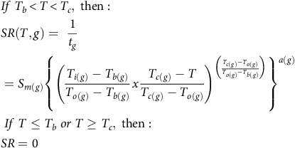 $$\eqalign{ & & If\;{T_b} \lt T \lt {T_c},{\rm{\;then}}:{\rm{\;}}\; \cr & & SR\left( {T,g} \right) = {\rm{\;}}{1 \over {{t_g}}} \cr & & = {S_{m\left( g \right)}}{\left\{ {{{\left( {{{{T_{i\left( g \right)}} - {T_{b\left( g \right)}}} \over {{T_{o\left( g \right)}} - {T_{b\left( g \right)}}}}x{{{T_{c\left( g \right)}} - T} \over {{T_{c\left( g \right)}} - {T_{o\left( g \right)}}}}} \right)}^{\left( {{{{T_{c\left( g \right)}} - {T_{o\left( g \right)}}} \over {{T_{o\left( g \right)}} - {T_{b\left( g \right)}}}}} \right)}}} \right\}^{a\left( g \right)}} \cr & & \;If\;T \le {T_b}\;or\;T \ge {T_c},\;{\rm{then}}: \cr & & SR = 0 \cr} $$
where SR is the sprouting rate calculated for each fragment length for each percentile and run (g), T is the sprouting temperature, a is a shaping parameter, and S m is the highest SR that occurs at the To . This model predicted no sprouting below Tb or above Tc .
Equation 2 estimates five parameters, and because there are five percentiles, the total number parameters estimated for each fragment length was 25. However, according to Mesgaran (Reference Mesgaran2018), the number of parameters in the prediction model can be reduced by using an equation that sets the same T b, T o, and T c values across the different percentiles, as follows:
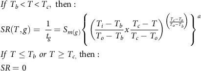 $$\eqalign{ & & If\;{T_b} \lt T \lt {T_c},\;{\rm{then}}:\;\; \cr & & SR\left( {T,g} \right) = \;{1 \over {{t_g}}} = {S_{m\left( g \right)}}{\left\{ {{{\left( {{{{T_i} - {T_b}} \over {{T_o} - {T_b}}}x{{{T_c} - T} \over {{T_c} - {T_o}}}} \right)}^{\left( {{{{T_c} - {T_o}} \over {{T_o} - {T_b}}}} \right)}}} \right\}^a} \cr & & If\;T \le {T_b}\;or\;T \ge {T_{c,}}\;{\rm{then}}:\;\; \cr & & SR = 0 \cr} $$
This model has nine parameters and is based on a positive relationship between the percentiles and the value of SR. Two more modeling approaches were also tested based on Equation 3. The first—with 13 parameters (Bradford Reference Bradford2002)—assumes fixed Tb and To parameters and a variable Tc parameter across the different percentiles. The second—with 13 parameters—assumes the fixed Tb and Tc parameters and a variable To parameter across the percentiles (Mesgaran et al. Reference Mesgaran, Onofri, Mashhadi and Cousens2017). For simplicity, we will refer to our four models as follows: the 25-parameter model is designated the “variable model,” the 9-parameter model is designated the “fixed Tc model,” and the two 13-parameter models are designated the “variable Tc model” and the “variable To model.” To determine potential data pooling between the two runs, the 95% confidence interval (CI) values of the estimated cardinal temperatures and a (the shape parameter) were compared for all four models.
Finally, the Akaike information criterion (AIC) was used to assess the models. This method compares the goodness of fit of the models; the model with the lowest AIC value was selected. The AIC method incorporates the amount of reduction of the residual sum of squares (RSS) and the model complexity (Burnham and Anderson Reference Burnham and Anderson2004):
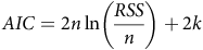 $$AIC = 2n\ln \left( {{{RSS} \over n}} \right) + 2k$$
where n is the number of observations, and k is the number of parameters used in the model.
Development of the Sprouting Dynamics Model
To develop a TT sprouting predictive model among fragment lengths at all temperatures, the cardinal temperatures from the favorable model—according to the AIC criterion—were used for computing GDD. The accumulated values over time (n) were estimated for each rhizome length using the following equation (Cochavi et al. Reference Cochavi, Rubin, Achdari and Eizenberg2016; Mesgaran Reference Mesgaran2018):
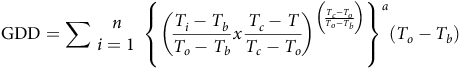 $${\rm{GDD}} = \sum \matrix{ n \cr {i = 1} \cr } {\rm{\;}}{\left\{ {{{\left( {{{{T_i} - {T_b}} \over {{T_o} - {T_b}}}x{{{T_c} - T} \over {{T_c} - {T_o}}}} \right)}^{\left( {{{{T_c} - {T_o}} \over {{T_o} - {T_b}}}} \right)}}} \right\}^a}\left( {{T_o} - {T_b}} \right)$$
where T i is the daily temperature for the ith day, and n is the total number of days for which GDD are to be calculated. Equation 5 takes into consideration the sub- and supra-optimal temperature ranges in the GDD accumulation. The response of S. elaeagnifolium sprouting to GDD was analyzed using a four-parameter Weibull equation:
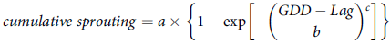 $$cumulative\;sprouting = a \times \left\{ {1 - \exp \left[ { - {{\left( {{{GDD - Lag} \over b}} \right)}^c}} \right]} \right\}$$
where a is the maximal sprouting, c is the shape parameter that determines the skewness and kurtosis of the equation, b is the scale parameter regardless of the shape value, and lag is the estimate of the time required for the sprouting of the first rhizome. The root-mean-square error (RMSE) was calculated as an indicator of goodness of fit (Lati et al. Reference Lati, Filin and Eizenberg2011; Mobli et al. Reference Mobli, Oliveira, Butts, Proctor, Lawrence and Werle2022).
Results and Discussion
Impact of Constant Temperatures on Solanum elaeagnifolium Sprouting
The sprouting of S. elaeagnifolium was adequately described using a log-logistic time-to-event model for all temperature regimes for each fragment length (Figure 1). However, the curve compression revealed significant differences between the two runs (P-value < 0.05) in 11 out of the 24 combinations of temperatures and fragment length model (Figure 1). Furthermore, the pairwise compression of the parameters derived from these 11 models also revealed significant differences (Supplementary Table S1). Thus, at this stage of the model development, the data were not pooled, and each run was analyzed separately.

Figure 1. Time-to-event, three-parameter log-logistic equation:
 $$f\left( t \right) = d/1 + {\rm{exp\{ }}b({\rm{log(}}t{\rm{)}} - {\rm{log(}}e{\rm{)}})\} $$
showing the relationship between constant temperature (C) and sprouting proportion of Solanum elaeagnifolium rhizomes of four different fragment lengths (2.5, 5, 7.5, and 10 cm) in the two runs, where d is the maximum sprouting, e is the time (days) at which 50% of the rhizomes had sprouted, and b is an absolute value proportional to the slope of f at time t. Coefficients for the equation parameters are presented in Table 1; n = 3. The P-value was calculated by the permutation approach to determine the difference between curves of the two runs. Curves were considered significantly different when the P-value was <0.05.
$$f\left( t \right) = d/1 + {\rm{exp\{ }}b({\rm{log(}}t{\rm{)}} - {\rm{log(}}e{\rm{)}})\} $$
showing the relationship between constant temperature (C) and sprouting proportion of Solanum elaeagnifolium rhizomes of four different fragment lengths (2.5, 5, 7.5, and 10 cm) in the two runs, where d is the maximum sprouting, e is the time (days) at which 50% of the rhizomes had sprouted, and b is an absolute value proportional to the slope of f at time t. Coefficients for the equation parameters are presented in Table 1; n = 3. The P-value was calculated by the permutation approach to determine the difference between curves of the two runs. Curves were considered significantly different when the P-value was <0.05.
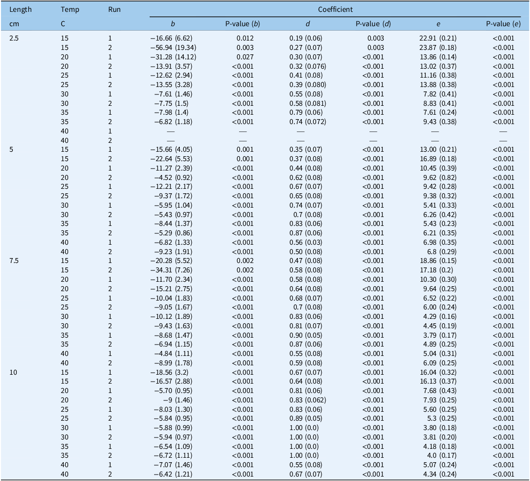
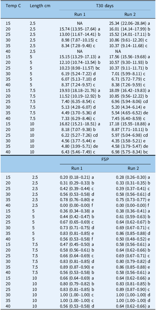
In both runs, there was no sprouting at the two extreme temperature regimes (10 and 45 C), but sprouting was observed starting from a temperature of 15 C, and the maximum sprouting (parameter d) was found to increase with fragment length. For example, in Run 1, this parameter reached values of 0.19, 0.35, 0.47, and 0.67 for the 2.5-, 5-, 7.5-, and 10-cm lengths, respectively, at 15 C (Table 1). Also in Run 1, the highest sprouting proportion was observed at 35 C, with the maximum sprouting reaching values of 0.79, 0.83, 0.90, and 1.00 for the 2.5-, 5-, 7.5-, and 10-cm lengths, respectively. In both runs, a decline in maximum sprouting was observed at 40 C, and for the 10-cm fragment length in Run 2, the value of this parameter dropped to 0.64 (Table 1). The time taken for 50% of the rhizomes to sprout (e parameter) was found to decrease with length for shorter versus longer fragments. In Run 2, for example, this parameter was the highest for all fragments at 15 C, reaching values of 23.8, 16.8, 17.1, and 16.1 d for the 2.5–, 5-, 7.5-, and 10-cm fragment lengths, respectively (Table 1). The e parameter declined as the temperature increased, with the lowest values being obtained at 30 and 35 C. In Run 1, the value of this parameter was 7.8 and 5.4 d for fragment lengths of 2.5 and 5 cm, respectively, while for the longer fragments of 7.5 and 10 cm, it was 4.1 and 3.8 d, respectively. The GLM analysis of the T30 values also revealed that the sprouting times of the longer fragments were significantly lower than those for the shorter ones in both runs (Table 2). For example, in Run 2, the T30 values at 25 C for the 7.5- and 10-cm fragments were ∼7 and ∼6 d, respectively. These values were significantly lower than those for the shorter fragments of 2.5 and 5 cm, with T30 values of 10.3 and 15.5 d, respectively. The shortest time to sprouting in Run 1 (i.e., 4.5 d) was observed at 35 C for the fragment length of 7.5 cm, while the shortest time to sprouting in Run 2 (i.e., 4.3 d) was observed at 30 C for fragments of 10 cm (Table 2).
Table 1. Coefficients and their standard errors (in parentheses) and P-values describing the relationship between sprouting at different constant temperature (C) regimes a and rhizome fragment lengths of Solanum elaeagnifolium in the two runs
a
A time-to-event, three-parameter log-logistic equation was used. Equation 1:
 $$f\left( t \right) = d/\{ 1 + {\rm{exp}}(b\left( {{\rm{log(}}t{\rm{)}} - {\rm{log(}}e{\rm{)}}} \right)\} $$
, where d is the maximum sprouting, e is the time (days) at which 50% of the rhizomes had sprouted, and b is an absolute value proportional to the slope of f at time t.
$$f\left( t \right) = d/\{ 1 + {\rm{exp}}(b\left( {{\rm{log(}}t{\rm{)}} - {\rm{log(}}e{\rm{)}}} \right)\} $$
, where d is the maximum sprouting, e is the time (days) at which 50% of the rhizomes had sprouted, and b is an absolute value proportional to the slope of f at time t.
Table 2. Influence of temperature (C) and rhizome fragment length (cm) on final sprouting proportion (FSP) and time to 30% sprouting (T30) for Solanum elaeagnifolium in the two runs with the 95% confidence intervals given in parentheses a
a
Values followed by the same letter are not significantly different according to multiple-comparison procedure with multiplicity adjustment (P
 $$\; \le \;$$
0.05).
$$\; \le \;$$
0.05).
Our results show the wide range of temperatures, namely, 15 to 40 C, under which S. elaeagnifolium rhizomes can sprout, with optimal sprouting occurring at the relatively high temperatures of 30 and 35 C. Similar results have been reported for other perennial weed species with subsoil dispersal organs that are typical for Mediterranean climate regions, such as bermudagrass [Cynodon dactylon (L.) Pers.] at 33 C (Satorre et al. Reference Satorre, Rizzo and Arias1996) and yellow nutsedge (Cyperus esculentus L.) at 28 C (Li et al. Reference Li, Shibuya, Yogo and Hara2000), indicating the preference for high temperatures for sprouting of such plants. Furthermore, our results indicate that the maximum sprouting of S. elaeagnifolium rhizomes was higher by 10 C than that for seed germination (Kapiluto et al. Reference Kapiluto, Eizenberg and Lati2022). In general, rhizomes contain larger carbohydrate reserves than seeds, which in turn enable them to survive and sprout in extreme environments (Anbari et al. Reference Anbari, Lundkvist and Verwijst2011; Chen et al. Reference Chen, Cao, Deng, Xie, Li, Hou and Li2015; Mangoale and Afolayan Reference Mangoale and Afolayan2020; Yu et al. Reference Yu, Chen and Dong2001). The rhizomes thus provide S. elaeagnifolium, like other perennial species, with a substantial advantage in terms of adaptability and colonization potential under Mediterranean and extreme climates (Travlos Reference Travlos2013; Uludag et al. Reference Uludag, Gbehounou, Kashefi, Bouhache, Bon, Bell and Lagopodi2016). In addition, we also observed that the longer rhizome fragments sprouted more rapidly, with higher FSP values (Table 2), regardless of temperature. These results can also be attributed to the larger carbohydrate reserves in the longer fragments. It is also likely that the longer rhizomes contain more buds, which contribute to the higher FSP values.
Modeling Sprouting Rate as a Function of Temperature
The fitted curves were used to derive the sprouting rates for the 10th, 20th, 30th, 40th, and 50th percentiles, which were used to parameterize Equation 1. By regarding the percentile g as a factor of the rhizome fragment (fragment size), we reached a total number of 25 parameters. In agreement with previous germination modeling studies, we tested three other modeling approaches with 9 (Washitani Reference Washitani1987) and 13 (Bradford Reference Bradford2002; Mesgaran et al. Reference Mesgaran, Onofri, Mashhadi and Cousens2017; Rowse and Finch-Savage Reference Rowse and Finch-Savage2003) parameters that enable the constant cardinal temperatures to be varied for all percentiles. Here, the 95% CI analysis revealed no significant differences between the estimates of the three cardinal temperatures and the shape parameters of the two runs. This trend was revealed in all four tested models, and thus, at this stage of the model development, data from the two runs were pooled (Supplementary Figure S1).
The computed AIC showed some differences between the accuracy levels of the four models. As Table 3 shows, the nine-parameter fixed T
c model provided the best fit, with the smallest AIC value in all rhizome fragment lengths, with the extracted values being: −1,309, −1,215, −1,191, and −1,219 for the rhizome lengths of 2.5, 5, 7.5, and 10 cm, respectively (Table 3). Thus, the fixed T
c model was used to determine the cardinal temperatures of the pooled data of the rhizome fragment lengths. The T
b values were 12.80
 $$\; \pm \;$$
1.01, 9.34
$$\; \pm \;$$
1.01, 9.34
 $$\; \pm \;$$
0.71, 9.14
$$\; \pm \;$$
0.71, 9.14
 $$\; \pm \;$$
1.87, and 9.50
$$\; \pm \;$$
1.87, and 9.50
 $$\; \pm \;$$
0.68, the T
o values were 38.9
$$\; \pm \;$$
0.68, the T
o values were 38.9
 $$0 \pm \;$$
0.07, 36.60
$$0 \pm \;$$
0.07, 36.60
 $$\; \pm \;$$
0.23, 35.16
$$\; \pm \;$$
0.23, 35.16
 $$\; \pm \;$$
0.57, and 34.86
$$\; \pm \;$$
0.57, and 34.86
 $$\; \pm \;$$
0.40, and the T
c values were 39.80
$$\; \pm \;$$
0.40, and the T
c values were 39.80
 $$\; \pm \;$$
0.07, 40.08
$$\; \pm \;$$
0.07, 40.08
 $$\; \pm \;$$
0.03, 40.50
$$\; \pm \;$$
0.03, 40.50
 $$\; \pm \;$$
0.40 and 40.80
$$\; \pm \;$$
0.40 and 40.80
 $$\; \pm \;$$
0.40 for the rhizome lengths of 2.5, 5, 7.5, and 10 cm, respectively. In addition, the S
m parameter decreased with the percentiles in all fragment lengths (Table 4). The values of the S
m parameter increased as the fragment length increased: for the 2.5-cm fragment length, this value was 0.18, 0.16, 0.14, 0.11, and 0.08, while for the 10-cm fragment length, this value was 0.36, 0.32, 0.29, 0.26, and 0.24 for the 10th, 20th, 30th, 40th, and 50th percentiles, respectively.
$$\; \pm \;$$
0.40 for the rhizome lengths of 2.5, 5, 7.5, and 10 cm, respectively. In addition, the S
m parameter decreased with the percentiles in all fragment lengths (Table 4). The values of the S
m parameter increased as the fragment length increased: for the 2.5-cm fragment length, this value was 0.18, 0.16, 0.14, 0.11, and 0.08, while for the 10-cm fragment length, this value was 0.36, 0.32, 0.29, 0.26, and 0.24 for the 10th, 20th, 30th, 40th, and 50th percentiles, respectively.
Table 3. Akaike information criterion (AIC), degrees of freedom (df), and number of parameters of the four models used (references in parentheses) to describe the relationship between sprouting rates and temperature of Solanum elaeagnifolium rhizome fragments of four different lengths
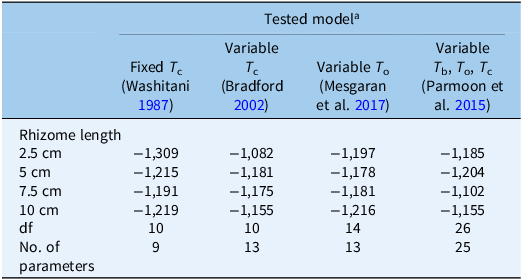
a T c, ceiling temperature, T o, optimum temperature, T b, base temperature.
Table 4. Influence of temperature on the sprouting rates for Solanum elaeagnifolium for the different percentiles of four different lengths for the pooled data
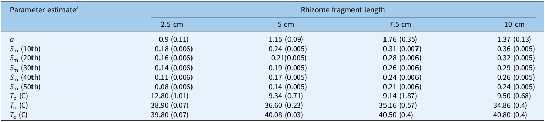
a Parameter estimates for Equation 3: T b, base temperature; T o, optimum temperature; T c, ceiling temperature; and the shape parameter of the equation that gives more flexibility to the model (a).
The modeling approaches used in this study take into consideration the different sprouting characteristics of the various percentiles within the rhizome fragment lengths (Figure 2). These differences were reflected by the S m parameter in Equation 3, which represents the maximal value of SR. Understanding the sprouting dynamics among different percentiles of S. elaeagnifolium allows for informed decision making in control activities. This insight enables precise targeting of control measures to the timing when the majority of the fragment has emerged, preventing both early and late applications.
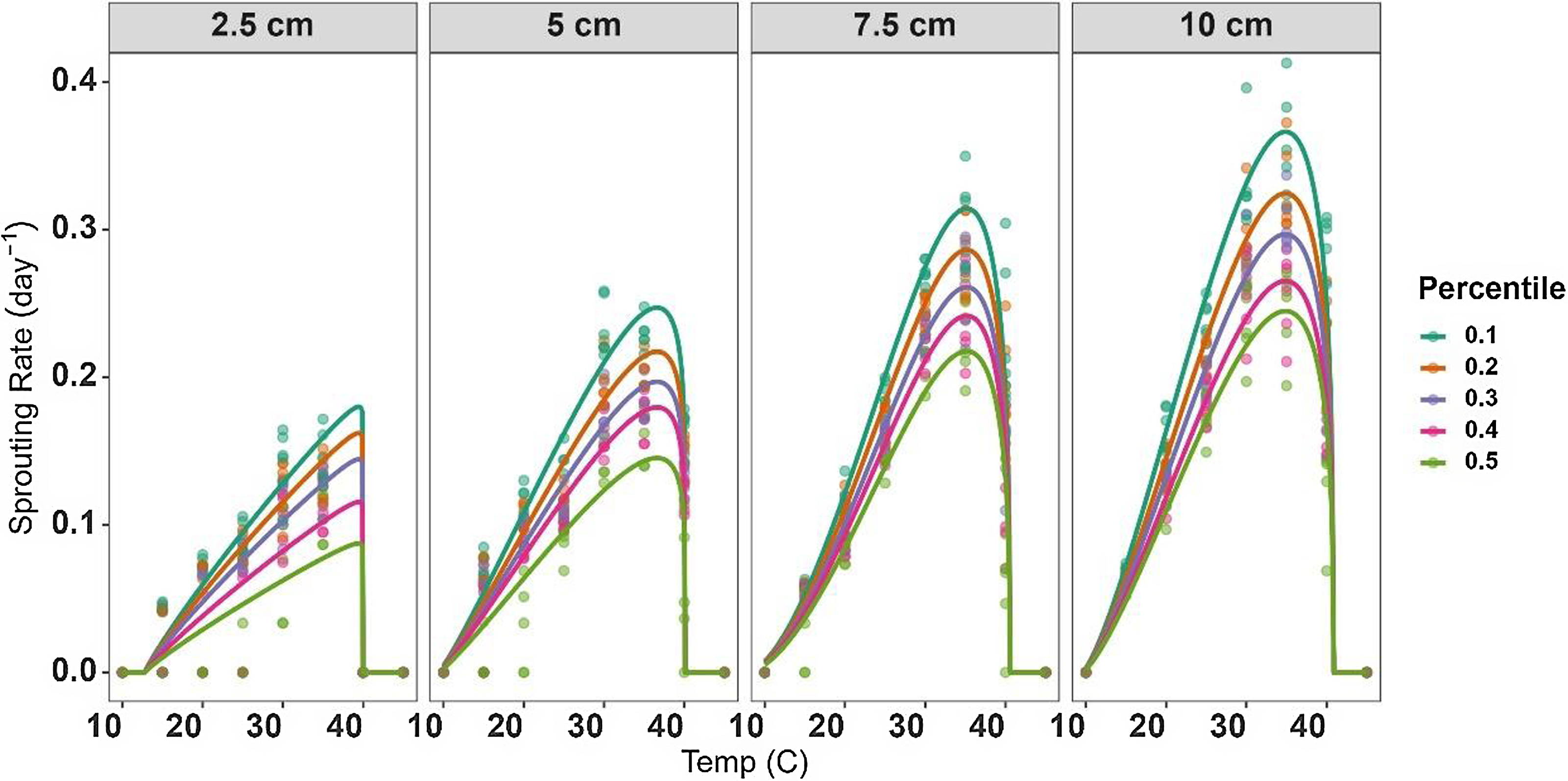
Figure 2. Relationship between sprouting rate (SR) of 10th, 20th, 30th, 40th, and 50th percentiles and temperature for Solanum elaeagnifolium rhizomes of four different fragment lengths (2.5, 5, 7.5, and 10 cm). Symbols show the observed data, while lines show the fitted curves (Equation 3) with the parameters given in Table 3.
The beta-function model was then used to predict S. elaeagnifolium sprouting rate among all rhizome lengths and was shown to be suitable for predicting the effects of temperature on the sprouting rate of this weed. The model’s effectiveness in predicting cardinal temperatures and the development of phenological events in various plant species has indeed been demonstrated previously (Cochavi et al. Reference Cochavi, Rubin, Achdari and Eizenberg2016, Reference Cochavi, Goldwasser, Horesh, Igbariya and Lati2018; Yin et al. Reference Yin, Kropff, McLaren and Visperas1995). Kapiluto et al. (Reference Kapiluto, Eizenberg and Lati2022), who performed a study similar to the current one, but for seeds, revealed cardinal temperatures of 10.8, 23.8, and 35.9 C for T b, T o, and T c, respectively. It may be seen that these values for S. elaeagnifolium seeds and rhizomes differed mainly for T o and T c, which were higher by 12 and 5 C, respectively, among the rhizome fragments. These results further emphasize the plasticity of S. elaeagnifolium and its ability to adapt to temperature variations, similar to other invasive species, and the importance of conducting studies focusing on rhizomes (Clements and DiTommaso Reference Clements and DiTommaso2011; Peters et al. Reference Peters, Breitsameter and Gerowitt2014). It can be assumed that the higher carbohydrate content in rhizome buds, compared with seeds, contributes to increased resistance to extreme temperatures. In light of the global warming trend, the implications of these results suggest that this species may colonize new areas that are currently characterized by moderate climates (Gioria and Pyšek Reference Gioria and Pyšek2017). It can be assumed that higher temperatures will affect seed germination in S. elaeagnifolium and that dispersal via rhizomes will be become the dominant path.
Development of the Sprouting Dynamics Model
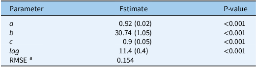
Following the extraction of the cardinal temperatures, a TT model for estimating cumulative S. elaeagnifolium sprouting was developed, using the pooled data for all temperature regimes and rhizome fragment lengths. Time (in days) was converted to GDD using Equation 5, and the cardinal temperatures derived from the fixed T c model were applied to the pooled data. As Figure 3 shows, the four-parameter Weibull equation adequately described the sprouting dynamics for S. elaeagnifolium with a RMSE of 0.154 and P-value of < 0.001 for all derived model parameters (Table 5). These results indicate the accurate sprouting prediction ability offered by the cardinal temperatures that were derived from the fixed T c model.
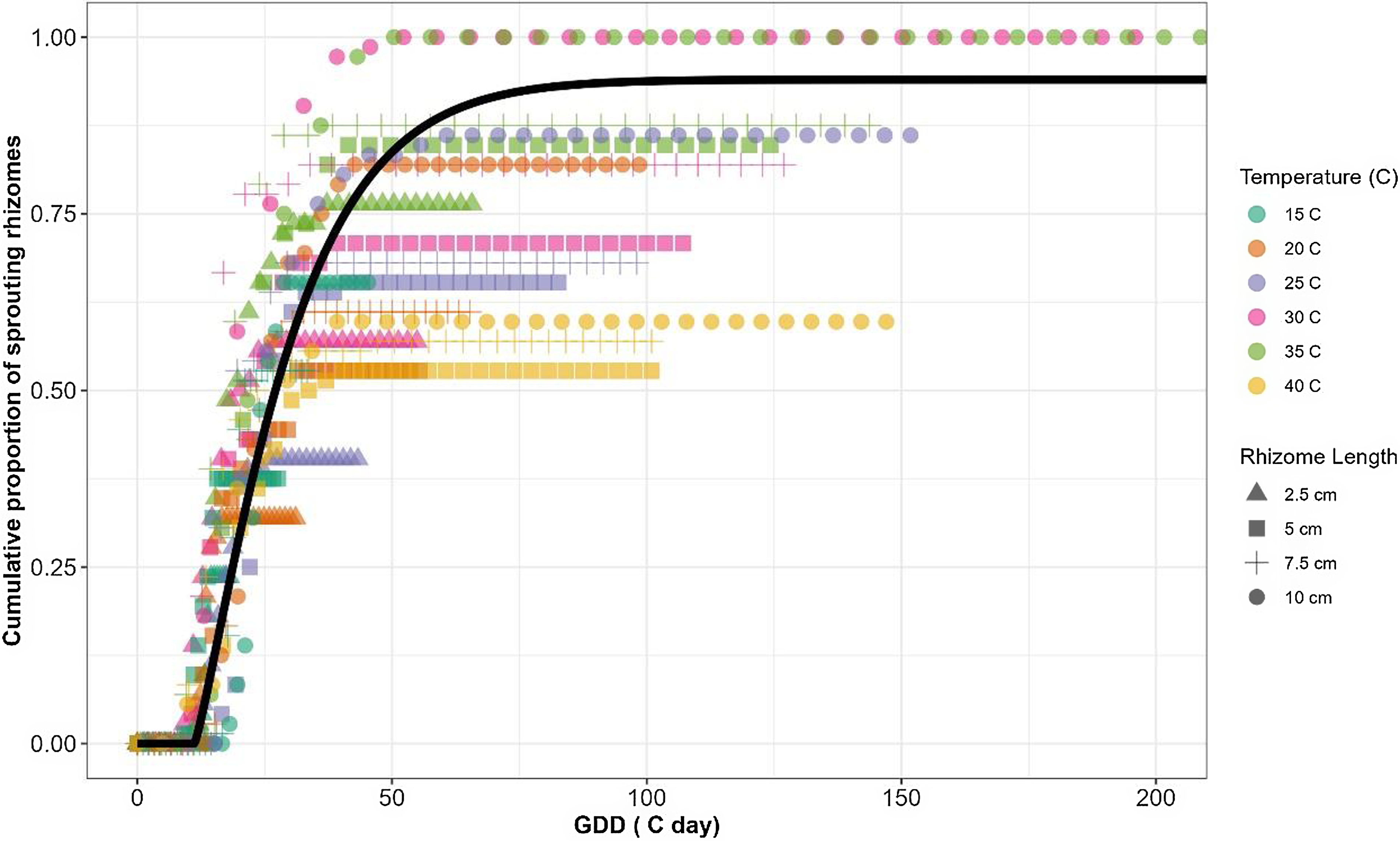
Figure 3. Sprouting dynamics of Solanum elaeagnifolium in relation to growing degree days (GDD) obtained using a four-parameter Weibull equation: f(GDD) = a[1 − exp(−{[(GDD − lag)/ b] c})], where a is maximal sprouting proportion, b is scale parameter regardless of the shape value, c is shape parameter that determines the skewness and kurtosis of the equation, and lag is estimate of the time required for the sprouting of the first rhizome. RMSE, root-mean-square error.
Table 5. Four-parameter Weibull equation describing the sprouting dynamics of Solanum elaeagnifolium in relation to growing degree days (GDD):
 $$\;{\rm{cumulative\;sprouting}} = a\left\{ 1 - {\rm{exp}}\left[ - {\left({{GDD - Lag} \over b}\right)^c}\right]\right\}$$
, where a is the maximal Solanum elaeagnifolium sprouting, b is the scale parameter regardless of the shape value, c is the shape parameter that determines the skewness and kurtosis of the equation, and lag is the estimate of the time required for the sprouting of the first rhizome
$$\;{\rm{cumulative\;sprouting}} = a\left\{ 1 - {\rm{exp}}\left[ - {\left({{GDD - Lag} \over b}\right)^c}\right]\right\}$$
, where a is the maximal Solanum elaeagnifolium sprouting, b is the scale parameter regardless of the shape value, c is the shape parameter that determines the skewness and kurtosis of the equation, and lag is the estimate of the time required for the sprouting of the first rhizome
a RMSE, root-mean-square error.
Based on the GDD computation (Equation 5) and the parameters that were determined via Equation 6, it was predicted that S. elaeagnifolium rhizomes have a lag time of 12 GDD, the 50% sprouting would be reached after almost ∼30 GDD, and the maximum sprouting would be recorded at 80 GDD (Figure 3). Kapiluto et al. (Reference Kapiluto, Eizenberg and Lati2022) showed that for seed germination, the GDD values of the lag, 50% germination, and the maximum germination stages were higher, ∼50, 140, and 180 GDD, respectively. These results further emphasize that rhizomes, as the main S. elaeagnifolium dispersal organ, contribute to the aggressiveness of this weed in agrosystems by rapid sprouting and establishment. The employment of a beta function for computing the GDD to estimate the sprouting rate of S. elaeagnifolium as related to TT allows the use of data obtained from the entire examined range of temperatures. To the best of our knowledge, this is the first time a beta function has been used to predict S. elaeagnifolium based on TT. The ability to predict rhizome sprouting patterns and dynamics in relation to GDD is an important biological tool that can facilitate optimized decision making for weed control timing; for example, the outcomes of cultivation and herbicide applications can be improved by leveraging their optimal timing estimated by modeling (Grundy Reference Grundy2003). However, to improve its practical application in the field, further research is required. One notable factor to consider is that the rhizomes remain buried in the soil, consistently exposed to local environmental conditions throughout various seasons. There is a gap in determining the initial timing for temperature measurement and GDD accumulation. Eizenberg et al. (Reference Eizenberg, Colquhoun and Mallory-Smith2004) approach this gap by proposing January 1 as the starting point for temperature measurement, hypothesizing that this period represents the coldest time of the year, when seeds are still dormant. This date could serve as a reference point in our system, particularly when rhizomes are dormant during low winter temperatures and initiate sprouting as temperatures rise.
The effectiveness of herbicides and mechanical tools, such as cultivation and harrowing, is markedly impacted by the weed phenology stage at the time of application. When weed control tactics are applied under favorable conditions (i.e., young buds), low herbicide rates and mechanical treatments can still provide satisfactory results (Kolberg et al. Reference Kolberg, Brandsæter, Bergkvist, Solhaug, Melander and Ringselle2018; Lati et al. Reference Lati, Filin and Eizenberg2012). Our findings regarding the phenology dynamics of S. elaeagnifolium can also be linked to—and improve—other practical weed control concepts, such as the critical period for weed control (CPWC), that is, the specific stage in a crop’s growth cycle at which controlling weeds is crucial to prevent yield loss (Knezevic et al. Reference Knezevic, Evans, Blankenship, Van and Lindquist2002). The competition between weed and crop is influenced by temperature conditions, and our findings can improve any CPWC model. Knowledge of the CPWC can enable farmers and land managers to effectively plan and execute weed control measures, ultimately leading to higher crop yields and improved ecosystem health (Knezevic and Datta Reference Knezevic and Datta2015).
In conclusion, our findings have important implications for predicting the future invasiveness of S. elaeagnifolium rhizomes under varying temperature conditions. Understanding the patterns of sprouting in S. elaeagnifolium is crucial for optimizing strategies to manage and control this weed. Here, we provide the first comprehensive analysis of its sprouting dynamics by using a precise beta-function model. The cardinal temperatures for sprouting were determined: T
b values were 12.8
 $$0 \pm \;$$
1.01, 9.34
$$0 \pm \;$$
1.01, 9.34
 $$\; \pm \;$$
0.71, 9.14
$$\; \pm \;$$
0.71, 9.14
 $$\; \pm \;$$
1.87, and 9.5
$$\; \pm \;$$
1.87, and 9.5
 $$0 \pm \;$$
0.68, the T
o values were 38.9
$$0 \pm \;$$
0.68, the T
o values were 38.9
 $$0 \pm \;$$
0.07, 36.60
$$0 \pm \;$$
0.07, 36.60
 $$\; \pm \;$$
0.23, 35.16
$$\; \pm \;$$
0.23, 35.16
 $$\; \pm \;$$
0.57 and 34.86
$$\; \pm \;$$
0.57 and 34.86
 $$\; \pm \;$$
0.40, and the T
c values were 39.80
$$\; \pm \;$$
0.40, and the T
c values were 39.80
 $$\; \pm \;$$
0.07, 40.08
$$\; \pm \;$$
0.07, 40.08
 $$\; \pm \;$$
0.03, 40.50
$$\; \pm \;$$
0.03, 40.50
 $$\; \pm \;$$
0.40, and 40.80
$$\; \pm \;$$
0.40, and 40.80
 $$\; \pm \;$$
0.40 for rhizome lengths of 2.5, 5, 7.5, and 10 cm, respectively. Importantly, these cardinal temperature values can be used to predict other phenological stages, thereby enhancing the implementation of weed control measures during later growth stages. As we strive for the adoption of new integrated weed management programs, it is vital to have the comprehensive biological data that will enable optimal outcomes. Further studies conducted under field conditions are thus critical to refine predictive emergence models developed using data obtained under laboratory conditions and to fine-tune weed control timing.
$$\; \pm \;$$
0.40 for rhizome lengths of 2.5, 5, 7.5, and 10 cm, respectively. Importantly, these cardinal temperature values can be used to predict other phenological stages, thereby enhancing the implementation of weed control measures during later growth stages. As we strive for the adoption of new integrated weed management programs, it is vital to have the comprehensive biological data that will enable optimal outcomes. Further studies conducted under field conditions are thus critical to refine predictive emergence models developed using data obtained under laboratory conditions and to fine-tune weed control timing.
Supplementary material
The supplementary material for this article can be found at https://doi.org/10.1017/wsc.2024.8.
Acknowledgment
The authors wish to thank the Chief Scientist of the Israel Ministry of Agriculture for funding this project (grant no. 20-02-0076). The authors declare that they have no conflicts of interest.


