


I. INTRODUCTION
The minimum variance distortionless response (MVDR) beamformer is known to maximize the output signal-to-interference-plus-noise ratio (SINR) by minimizing the total beamformer output power subject to a distortionless constraint for the signal. If the training data contain the signal component, the MVDR beamformer becomes a minimum power distortionless response (MPDR) beamformer, so even a small mismatch in the signal' steering vector (SSV) and/or array covariance matrix can lead to a severe degradation of the performance [Reference Wax and Anu1]. In practice, such a mismatch can be caused by the pointing error [Reference Liu, Jian, Du and Bai2], calibration errors [Reference Tseng, Feldman and Griffiths3]), unknown wavefront distortions [Reference Weiss and Friedlander4], local scattering [Reference Pedersen, Mogensen and Fleury5], moving target [Reference Yermeche, Grbic and Claesson6], etc. Finite sampling sequence [Reference Mestre and Lagunas7] also leads to inaccurate covariance matrix. Therefore, the robustness technology [Reference Li and Stoica8] is required to overcome these problems. We refer to the beamformer that attempts to preserve good performance in the presence of mismatch as robust adaptive beamformer (RAB). A minimal goal for RAB is that its performance should never degrade below the performance of a conventional beamformer.
In past two decades, many technologies have been developed to improve the robustness of the MPDR beamformer against the SSV mismatch. They are mainly divided into two types. The first type technology imposes additional constraints on the beamformer to prevent or decrease the signal self-nulling, and they can be divided into two categories: (1) The SSV updating approach updates the SSV estimated from prior parameters to make it get closer to actual SSV. Many algorithms are effective, such as the eigenspace projection approach [Reference Youn and Un9], the Bayesian approach [Reference Bell, Ephraim and Van Trees10], and the Taylor series approximation approach [Reference Er and Ng11]. However, actual SSV cannot be obtained, because the parameters that the algorithm uses are not accurate. (2) The robust constrained approach does not require actual SSV. It generally uses the SSV error norm constraint or beampattern constraint, such as the worst-case performance optimization-based beamformer (WCB) [Reference Vorobyov, Gershman and Luo12], the covariance fitting (CF)-based beamformer [Reference Li, Stoica and Wang13], and the multiple uncertainty sets constraint beamformer [Reference Yang, Liao, Xu, Zhu and Cao14]. The constrained beamformers generally have two problems: firstly, actual SSV error is difficult to obtain in practice [Reference Li, Ma, Yu and Cheng15]; secondly, the constraint is usually a second-order cone program problem, therefore it does not have closed-form solution [Reference Li, Ma and Cheng16]. Actually, most of the constrained robust adaptive beamformers turn out to be equivalent and belong to the extended class of diagonal loading (DL) approach [Reference Li, Stoica and Wang13]. When a RAB equivalents to the DL approach, another problem comes: the DL level is hard to choose in practice, and the RAB achieves better signal enhancement at the cost of losing its interference suppression capability, especially when the signal-to-noise ratio (SNR) is high. (2) The second type of robust technology is to eliminate or reduce the desired signal component before estimating the covariance matrix [Reference Gu and Leshem17,Reference Igambi, Yang and Jalal18]. Once the desired signal component is completely eliminated, the MPDR beamformer becomes an MVDR beamformer. Recently, some RABs based on the interference-plus-noise covariance matrix (INCM) reconstruction technology are proposed [Reference Liu, Jian, Du and Bai2,Reference Gu and Leshem17,Reference Lu, Li, Gao and Zhang19–Reference Zhang, Wei, Wen, Wang and Shi21]. The performance of the INCM-based RAB is almost always close to the optimal value across a wide range of SNR and signal-to-interference ratio (SIR). Unfortunately, the performance is severely degraded when array perturbations exist.
Most of the past studies used the SINR as the measure of system performance. However, SINR is not always the best measure performance, in some applications, SIR performance is more important [Reference Ganz, Moses and Wilson22]. In this paper, we develop a novel beamformer with enhancing the interference suppression capability at high input SNR. We call the proposed RAB as interference suppression robust adaptive beamformer (ISRAB). The main idea of ISRAB is that the suppression on the interference is enhanced as the input SNR gets larger. Three technologies, INCM reconstruction, covariance fitting, and worst-case performance optimization are used in ISRAB to guarantee enhancing the interference suppression capability.
The main contributions of this paper are listed as follows: (1) A RAB with enhancing the interference suppression capability is developed; (2) The working principle of the proposed ISRAB is analyzed, the feature of the ISRAB varies adaptively with the vary of input SNR; (3) A new steering vector which is close to actual SSV as well as orthogonal to the interference is estimated, perhaps it has potential uses for other applications.
The paper is organized as follows. The signal model and background on adaptive beamforming are presented in Section II. The theatrical analysis of the proposed ISRAB and its implementation is developed in Section III. Some simulation examples are shown in Section IV. Finally, a brief conclusion is given in Section V. In the following,  $E[\centerdot]$, $(\centerdot)^{T}$, $(\centerdot)^{H}$, $(\centerdot)^{-1}$, $\Vert \centerdot \Vert$, and ⊥ denote the expectation, transpose, Hermitian transpose, inverse, the two-norm, and orthogonal respectively, superscript $\hat {\cdot }$ denotes the estimated value.
II. PROBLEM FORMULATION
Considering one signal and P uncorrelated, narrowband interference impinge on a uniform linear array (ULA) with M omni-directional sensors located at x-axis in Cartesian coordinate system, P+1<M. The received data at k-th snapshot can be expressed as
 $${\bf x}(k)={{{\bf a}}_{0}}{{s}_{0}}(k)+\sum\nolimits_{i=1}^{P}{{{{\bf a}}_{i}}{{s}_{i}}(k)}+{\bf n}(k),$$
where a0 and  ${{{\bf a}}_{i}} = \exp \{j(2{\pi}/{\lambda}){{{\bf P}}^{T}}{{{\bf A}}_{i}}(\theta )\}$, $i=1,\, \ldots, \,P$, are the steering vectors of the desired signal and i-th interference respectively; ${\lambda }$ is the wavelength; ${\bf P}=[{{{\bf P}}_{1}},\,{{{\bf P}}_{2}},\, {\ldots }{{{\bf P}}_{M}}]$, Pm = [p xm, p ym, p zm]T, $m=1,\,2,\, {\ldots },\,M$, is each sensor's axis location; ${{{\bf A}}_{i}(\theta )}={{[{\rm cos(}{{{\theta }}_{i}}{\rm ),\,}{\rm sin(}{{{\theta }}_{i}}{\rm ),\,}{\rm 0}]}^{T}}$, ${{{\theta }}_{i}}$ is the angle between the direction-of-arrival (DOA) of i-th signal or interference and the axis of the ULA. s 0(k) and s i(k) are zero-mean stationary, n(k) denotes the noise.
The covariance matrix of the array output is given by
 $$\eqalign{{\bf R}&=E[{\bf x}(k){{{\bf x}}^{H}}(k)]\cr &={\sigma}_{0}^{2}{{{\bf a}}_{0}}{\bf a}_{0}^{H}+\sum\nolimits_{i=1}^{P}{{\sigma }_{i}^{2}{{{\bf a}}_{i}}{\bf a}_{i}^{H}}+ {\sigma }_{n}^{2}{{{\bf I}}_{M}},}$$
where  ${\sigma }_{0}^{2}$, ${\sigma }_{i}^{2}$, and ${\sigma }_{n}^{2}$ denote the power of signal, i-th interference, and noise, respectively.
The problem of maximizing the output SINR is mathematically equivalent to the problem
 $$ \mathop{\min}\limits_{\bf w} {{\bf w}^{H}}{{{\bf R}}_{IN}}{\bf w}\quad s.t.\quad {{{\bf w}}^{H}}{{{\bf a}}_{0}}=1,$$
where  ${\bf w}={{[{{w}_{1}},\, {\ldots },\,{{w}_{M}}]}^{T}}$ is the beamformer's weight vector, ${{{\bf R}}_{IN}}=\sum \nolimits _{i=1}^{P}{{\sigma }_{i}^{2}{{{\bf a}}_{i}}{\bf a}_{i}^{H}}+{\sigma }_{n}^{2}{{{\bf I}}_{M}}$ is the actual INCM. The solution of (3) is the MVDR beamformer
 $$ {{{\bf w}}_{opt}}={\alpha }{\bf R}_{IN}^{-1}{{{\bf a}}_{0}}{,} $$
where  ${\alpha }={{({\bf a}_{0}^{H}{\bf R}_{IN}^{-1}{{{\bf a}}_{0}})}^{-1}}$ is a normalization constant which does not affect the output SINR.
When the receiving snapshots include the desired signal component, RIN in (4) is replaced by R, then the MVDR becomes the MPDR:  ${{{\bf w}}_{MPDR}}={\alpha }{{{\bf R}}^{-1}}{{{\bf a}}_{0}}$, where ${\alpha }={{({\bf a}_{0}^{H}{{{\bf R}}^{-1}}{{{\bf a}}_{0}})}^{-1}}$. Although the MPDR has the same SINR performance with the MVDR, however, we cannot obtain two accurate parameters in practice. On one hand, since R is unknown in practice, it is replaced by K-snapshots sample covariance matrix $\hat {{\bf R}}=({1}/{K})\sum \nolimits _{k=1}^{K}{{\bf x}(k){{{\bf x}}^{H}}(k)}$. On the other hand, many factors can lead to the steering vector mismatch, such as the pointing error and the array perturbations (the perturbations often include the array element position error, calibration magnitude error, and calibration phase error), they can be modeled as [Reference Van Trees23]
 $$ \eqalign{{{{\bf a}}_{i}}(\theta )=&(1+\Delta g){{e}^{j\Delta {\phi }}}{{e}^{j(2{\pi }/{\lambda }){{({\bf P}+\Delta {\bf P})}^{T}}{{{\bf A}}_{i}}(\theta +\Delta \theta )}} \cr \Delta {\bf P}=&[\Delta {{{\bf P}}_{1}},\Delta {{{\bf P}}_{2}},{\ldots}\Delta {{{\bf P}}_{M}}] \cr \Delta {{{\bf P}}_{m}}=&{{[{{\Delta }_{xm}},{{\Delta }_{ym}},{{\Delta }_{zm}}]}^{T}},m=1,2,{\ldots},M,} $$
where Δθ, Δg,  $\Delta {\phi }$, and ΔP denote the pointing error, calibration magnitude error, calibration phase error, and array element position error, respectively. In this paper, we focus on the steering vector error, so the influence of covariance matrix is omitted, thus we do not distinguish R and $\hat {{\bf R}}$ in the following.
The inaccurate of covariance matrix of steering vector can lead to the output SINR significant decrease which is called self-nulling, especially when the input SNR is high. Many robust technologies have been developed to deal with this problem, one of the most popular method is called DL. The DL technique augments the diagonal of the covariance with a constant level
 $$ {{{\bf w}}_{DL}}={{({{{\bf R}}_{IN}}+{\beta }{\bf I})}^{-1}}{{{\bf a}}_{0}}{,} $$
where  ${\beta }$ is the DL level.
The DL technology has many useful effects, such as making the covariance matrix invertible, constraining the white noise gain [Reference Elnashar, Elnoubi and El-Mikati24], robust against the steering vector error and the covariance matrix error [Reference Zhang and Liu25], etc. However, the DL technology has some problems such as the DL level is hard to be chosen [Reference Elnashar, Elnoubi and El-Mikati24] and the interference suppression capability is reduced [Reference Ganz, Moses and Wilson22]. Some robust adaptive beamformers, such as the famous WCB and CFRCB have been proved and belong to the class of DL technology [Reference Vorobyov, Gershman and Luo12,Reference Li, Stoica and Wang13], therefore they have the same problems.
Most of the past studies used the SINR as the measure of system performance. However, SINR is not always the best measure performance, in some applications, SIR performance is more important [Reference Ganz, Moses and Wilson22]. In the following, we develop a novel beamformer ISRAB with enhancing the interference suppression capability.
III. THE PROPOSED BEAMFORMER
The ISRAB is developed with three steps: the INCM reconstruction technology is used to construct a subspace which is orthogonal to the interference; the CF technology is used to estimate an SV which is close to the desired signal's SV as well as orthogonal to the interference; the WCB technology is used to solve the weight vector to prevent self-nulling. Although three exist technologies are used, the form or usage in ISRAB is difference from their original complete solution.
A) Interference orthogonal subspace construction
Firstly, the INCM RIN is reconstructed with R through [Reference Gu and Leshem17]
 $$ {{{\bf R}}_{IN}}=\displaystyle{1 \over N}\sum\limits_{i=1}^{N}{\displaystyle{\hat{{\bf a}}({{{\theta }}_{i}}){{{\hat{{\bf a}}}}^{H}}({{{\theta }}_{i}}) \over {{{\hat{{\bf a}}}}^{H}}({{{\theta }}_{i}}){{{\hat{{\bf R}}}}^{-1}}\hat{{\bf a}}({{{\theta }}_{i}})}},{{{\theta }}_{i}}\in \bar{\Theta }{,} $$
where  $\hat {{\bf a}}({{{\theta }}_{i}})$ is the presumed steering vector corresponding to direction ${{{\theta }}_{i}}$, $\bar {\Theta }$ denotes the complement of signal uncertainty region Θ.
Taking the eigen-decomposition of RIN
 $$\eqalign{{{{\bf R}}_{IN}}&={{{\bf E}}_{I}}{{{\bf \Gamma }}_{I}}{\bf E}_{I}^{H}{\rm +}{{{\bf E}}_{N}}{{{\bf \Gamma }}_{N}}{\bf E}_{N}^{H} \cr & =\sum\limits_{i=1}^{P}{{{{\gamma}}_{i}}{{{\bf e}}_{i}}{\bf e}_{i}^{H}}+{{{\gamma }}_{n}}\sum\limits_{i=P+1}^{M}{{{{\bf e}}_{i}}{\bf e}_{i}^{H}},} $$
where  ${{{\gamma }}_{i}}$ and ei are the eigenvalues and corresponding eigenvectors of RIN, the eigenvalues are sorted in descending order ${{{\gamma }}_{1}}\ge {\ldots }\ge {{{\gamma }}_{P}}\gg {{{\gamma }}_{P+1}}= {\ldots }={{{\gamma }}_{M}}={\sigma }_{n}^{2}$, ${{{\bf E}}_{I}} = [{{{\bf e}}_{1}},\, {\ldots },\,{{{\bf e}}_{P}}]$ spans the interference subspace, ${{{\bf E}}_{N}} = [{{{\bf e}}_{P+1}}, {\ldots},{\bf e}_{M}]$ spans the noise subspace. The following formulas hold
 $${\rm span}\{{{{\bf a}}_{i}}\}={\rm span}\{{{{\bf e}}_{i}}\},i=1, {\ldots},P,$$
 $${{{\bf E}}_{I}}\bot{{{\bf E}}_{N}},{{{\bf E}}_{I}}{\bf E}_{I}^{H}{\rm +}{{{\bf E}}_{N}} {\bf E}_{N}^{H}{\rm =}{\bf I}{.}$$
 Therefore, the subspace  ${{{\bf E}}_{N}} = [{{{\bf e}}_{P+1}},\, {\ldots },\,{{{\bf e}}_{M}}]$ is orthogonal to each ISV.
B) Steering vector estimation
When the angular separation between signal and interference is larger than a beam width,  ${{\left \vert {\bf a}_{0}^{H}{{{\bf a}}_{i}}/M \right \vert}^{2}}\ll 1$, $i=1,\, {\ldots },\,P$ [Reference Chang and Yeh26]. Assuming this condition always holds, we can make the approximation ${{\left \vert {\bf a}_{0}^{H}{{{\bf e}}_{i}} \right \vert}^{2}}\ll M$, $i=1,\, {\ldots },\,P$, and ${\bf a}_{0}^{H}{{{\bf E}}_{I}}{\bf E}_{I}^{H}{{{\bf a}}_{0}}\ll M$, which can be further extended to ${\bf a}_{0}^{H}{{{\bf E}}_{N}}{\bf E}_{N}^{H}{{{\bf a}}_{0}} ={\bf a}_{0}^{H}({\bf I}-{{{\bf E}}_{I}}{\bf E}_{I}^{H}) {{{\bf a}}_{0}}=M-{\bf a}_{0}^{H}{{{\bf E}}_{I}}{\bf E}_{I}^{H}{{{\bf a}}_{0}}\approx M$. Therefore, we can make ${{\left\Vert {\bf E}_{N}^{H}{{{\bf a}}_{0}} \right\Vert}^{2}}\approx M$. Because ${{\left\Vert {{{\bf a}}_{0}} \right\Vert}^{2}} = M$, a0 approximately belongs to the subspace span{ei}, $i=P+1,\, {\ldots },\,M$. Hence, we can express the new SSV with the linear combination of ei, $i=P+1,\, {\ldots },\,M$
 $$ {{\hat{{\bf a}}}_{0}}\approx {{{\bf E}}_{N}}{\bf b}{,} $$
where b is an (M − P) × 1 dimensional rotating vector.
The CF technology [Reference Li, Stoica and Wang13] can be used to solve b
 $$\mathop{\min}\limits_{\hat{\bf a}_{0}} \hat{\bf a}_{0}^{H} {\bf R}^{-1} \hat{\bf a}_{0} \quad s.t. \quad \left\Vert \hat{\bf a}_{0} \right\Vert^{2} = M.$$
Using (11) and  ${\bf E}_{N}^{H} {\bf E}_{N} = {\bf I}_{M-P}$, equation (12) becomes
 $$ \mathop{\min}\limits_{\bf b} {\bf b}^{H} {\bf R}_{E} {\bf b} \quad s.t. \quad {\bf b}^{H} {\bf b} =M,$$
where  ${{{\bf R}}_{E}}={\bf E}_{N}^{H}{{R}^{-1}}{{{\bf E}}_{N}}$. The vector b can be solved by the Lagrange multiplier method
 $$ f({\bf b},{\eta })={{{\bf b}}^{H}}{{{\bf R}}_{E}}{\bf b}+{\eta }({{{\bf b}}^{H}}{\bf b}-M){,} $$
where  ${\eta }$ is the Lagrange multiplier. Differentiating of (14) with respect to b and equating the result to zero, the solution to (13) is given by the following generalized eigenvalue problem
 $$ {{{\bf R}}_{E}}{\bf b}={\eta }{\bf b}{.} $$
The solution to (15) is
 $${\bf b} = {\cal M}\{{\bf R}_{E}\},$$
where  ${\cal M}\{\centerdot \}$ is the operator that yields the eigenvector corresponding to the minimal eigenvalue.
Notice that the vector should be scaled to guarantee  $\left\Vert \hat{\bf a}_{0} \right\Vert = \sqrt{M}$. Therefore, the estimated new SSV is given by
 $$\hat{\bf a}_{0} = \sqrt{M} {\bf E}_{N} {\bf b}/\left\Vert {\bf E}_{N} {\bf b} \right\Vert.$$
 Obviously,  $\hat{\bf a}_{0}$ is close to actual SSV as well as orthogonal to each ISV.
We make the following two remarks:
Remark 1 Estimating an accurate noise subspace in (8) is not necessary. We can choose the eigenvectors corresponding to P EN(P EN ≤ M − P) small eigenvalues as the columns of EN. The weak interference component corresponding to the eigenvalues between P EN and M−P can be suppressed. An easy way to estimate P EN is to choose a maximal value of P EN which satisfies that the value of  $\ \sum \nolimits _{i=1}^{M-{{P}_{EN}}}{{{{\gamma }}_{i}}}$ divided by $\sum \nolimits _{i=1}^{M}{{{{\gamma }}_{i}}}$ is larger than a fixed value, such as 0.9.
Remark 2 The CF approach in [Reference Li, Stoica and Wang13] subjects to the constraint  ${{\left\Vert {{{\bf a}}_{CF}}-\hat {{\bf a}}({{{\hat {{\theta }}}}_{0}}) \right\Vert}^{2}}\le {\varepsilon }$ to search the maximal spatial power in SSV uncertainty region, where ${{\hat {\theta }}_{0}}$ is the presumed DOA of signal. The objective function of (12) searches the max spatial power through all the directions. Since ENb is orthogonal to the ISV, ${{\hat {{\bf a}}}_{0}}$ will not converge to any ISV. If SNR is high, ${{\hat {{\bf a}}}_{0}}$ will converge to the SSV. If SNR is very low, the signal power is submerged by the noise power in spatial spectrum, ${{\hat {{\bf a}}}_{0}}$ may converge to a noise power peak. The following stopping criterion is used to avoid that ${{\hat {{\bf a}}}_{0}}$ converges to the noise peak which is far from actual signal DOA: if $\left\vert \hat {{\bf a}}_{0}^{H}\hat {{\bf a}}({{{\hat {{\theta }}}}_{0}}) \right\vert <\min \{ \left\vert \hat {{\bf a}}_{0}^{H}\hat {{\bf a}}({{{\hat {{\theta }}}}_{0}}+{{{\theta }}_{W}}/2) \right\vert,\,\left\vert \hat {{\bf a}}_{0}^{H}\hat {{\bf a}}({{{\hat {{\theta }}}}_{0}}-{{{\theta }}_{W}}/2) \right\vert \}$, setting ${{\hat {{\bf a}}}_{0}}$ = $\hat {{\bf a}}({{\hat {{\theta }}}_{0}})$, where ${{{\theta }}_{W}}$ is the signal's DOA uncertainty range [Reference Nai, Ser, Yu and Chen27]. The criterion means that if the corresponding angle of ${{\hat {a}}_{0}}$ is beyond the signal DOA uncertainty range, using initial value $\hat{\bf a}(\hat{\theta}_{0})$ as ${{\hat {{\bf a}}}_{0}}$.
C) Solving the weight
The worst-case performance optimization-based beamformer can be formulated as [Reference Vorobyov, Gershman and Luo12]
 $$\left\{\matrix{& \mathop{\min}\limits_{\bf w} {\bf w}^{H} {\bf Rw} \hfill \cr & s.t. \left\vert {\bf w}^{H}(\hat{\bf a}_{0} + {\bf \delta}) \right\vert \ge 1, \forall \left\vert {\bf \delta} \right\vert \le {\varepsilon}\hfill},\right.$$
where δ is the vector of the unknown mismatch between the actual SSV and its presumed value  ${{\hat {{\bf a}}}_{0}}$ with a prior known norm bound ${\varepsilon }$. The solutions to (18) belongs to the DL approach [Reference Zarifi, Shahbazpanahi, Gershman and Luo28]
 $$ {\bf w}={{({\bf R}+{{\varepsilon }}/{{\tau }}\;{{{\bf I}}_{M}})}^{-1}}{{\hat{{\bf a}}}_{0}}{,} $$
where  ${\tau }$ is the root to
 $$\sum\limits_{i=0}^{M-1} \displaystyle{\left\vert {\bf q}_{i}^{H} \hat{\bf a}_{0} \right\vert^{2} \over (\varepsilon + \tau \lambda_{i})^2} = 1,$$
where  ${\bf R}=\sum \nolimits _{i=0}^{M-1}{{{{\lambda }}_{i}}{{{\bf q}}_{i}}{\bf q}_{i}^{H}}$, ${{{\lambda }}_{i}}$ and qi are the eigenvalues and corresponding eigenvectors of R, ${{{\lambda }}_{i}}$ are sorted in descending order ${{{\lambda }}_{0}}\ge {{{\lambda }}_{1}}\ge {\ldots }\ge {{{\lambda }}_{P+1}}= {\ldots }={{{\lambda }}_{M-1}}={{{\lambda }}_{n}}$. The binary search technique [Reference Zarifi, Shahbazpanahi, Gershman and Luo28] can be used to solve (20).
D) Working principle
Eigenvectors in noise subspace are approximately orthogonal to  ${{\hat {{\bf a}}}_{0}}$
 $$ {\bf q}_{i}^{H}{{\hat{{\bf a}}}_{0}}\approx 0, \ i=P+1,{\ldots},M-1{.} $$
In the following, we assume that the interference's number is equal to one so as to obtain a theoretical result. Simulation example 1 will show that when the interference number is larger than one, the theoretical result also establishes. The R with only one interference can be expressed in eigen-decomposition form
 $$ \eqalign{{\bf R}&={{{\lambda }}_{0}}{{{\bf q}}_{0}}{\bf q}_{0}^{H}+{{{\lambda }}_{1}}{{{\bf q}}_{1}}{\bf q}_{1}^{H}+\sum\limits_{i=2}^{M-1}{{{{\lambda }}_{n}}{{{\bf q}}_{i}}{\bf q}_{i}^{H}} \cr & =({{{\lambda }}_{0}}-{{{\lambda }}_{n}}){{{\bf q}}_{0}}{\bf q}_{0}^{H}+({{{\lambda }}_{1}}-{{{\lambda }}_{n}}){{{\bf q}}_{1}}{\bf q}_{1}^{H}+{{{\lambda }}_{n}}{{{\bf I}}_{M}}.} $$
Meanwhile, R can be expressed in array signal form
 $$ {\bf R}\approx {\sigma }_{0}^{2}{{\hat{{\bf a}}}_{0}}\hat{{\bf a}}_{0}^{H}+{\sigma }_{1}^{2}{{{\bf a}}_{1}}{\bf a}_{1}^{H}+{\sigma }_{n}^{2}{{{\bf I}}_{M}}{.} $$
By combining (22) and (23),  ${{{\lambda }}_{0}}$ and ${{{\lambda }}_{1}}$ can be solved [Reference Chang and Yeh26]
 $$\eqalign{\lambda_{0} &={\sigma}_{n}^{2}+\displaystyle{M \over 2}\left[{\sigma}_{0}^{2}+{\sigma }_{1}^{2} \right. \cr & \quad + \left. \sqrt{{{({\sigma }_{0}^{2}+{\sigma }_{1}^{2})}^{2}}-4{\sigma }_{0}^{2}{\sigma }_{1}^{2}(1-{{\left\vert v \right\vert}^{2}})} \right],}$$
 $$\eqalign{\lambda_1 & ={\sigma}_{n}^{2} + \displaystyle{M \over 2} \left[{\sigma}_{0}^{2} + {\sigma}_{1}^{2} \right. \cr & \quad - \left. \sqrt{({\sigma }_{0}^{2} + {\sigma}_{1}^{2})^{2} - 4{\sigma}_{0}^{2}{\sigma}_{1}^{2}(1-\left\vert v \right\vert^{2})} \right],}$$
 $$\left\vert {\bf q}_{i}^{H} \hat{\bf a}_{0} \right\vert^{2} = M(\!-1)^{i+1} \displaystyle{-{\lambda}_{i} + M {\sigma}_{1}^{2}(1 - \left\vert v \right\vert^{2}) \over {\lambda}_{0} - \lambda_1}, i = 0,1,$$
where λ0 > λ1,  $\left\vert v \right\vert^{2} = \left\vert \hat {\bf a}_{0}^{H} {\bf a}_{i}/M \right\vert^{2}\ll 1$, which is similar with the condition presented in Section III.B.
Case 1: Very high SNR
If  ${\sigma }_{0}^{2}\gg {\sigma }_{1}^{2}$, we can make
 $$\left\vert {\bf q}_{0}^{H} \hat{\bf a}_{0} \right\vert^{2} \approx M, \left\vert {\bf q}_{1}^{H} \hat{\bf a}_{0} \right\vert^{2} \approx 0.$$
If  ${\varepsilon }$ approaches $\sqrt {M}$ (we set $\varepsilon =0.99\sqrt {M}$ in the following), the denominators of (20) can satisfy
 $$ {{\left( {\varepsilon }+{\tau }{{{\lambda }}_{i}} \right)}^{2}}>M, \quad i=0,1,{\ldots},P{.} $$
From (20), (21), (27), and (28) we have
 $$ 1=\sum\limits_{i=0}^{M-1}{\displaystyle{{{\left\vert {\bf q}_{i}^{H}{{{\hat{{\bf a}}}}_{0}} \right\vert}^{2}} \over {{({\varepsilon }+{\tau }{{{\lambda }}_{i}})}^{2}}}}\approx \displaystyle{{{\left\vert {\bf q}_{0}^{H}{{{\hat{{\bf a}}}}_{0}} \right\vert}^{2}} \over {{({\varepsilon }+{\tau }{{{\lambda }}_{0}})}^{2}}}\approx \displaystyle{M \over {{({\varepsilon }+{\tau }{{{\lambda }}_{0}})}^{2}}}{.} $$
Equation (29) further reveals that
 $$ \displaystyle{{\varepsilon } \over {\tau }{{{\lambda }}_{0}}}\approx \displaystyle{{\varepsilon } \over \sqrt{M}-{\varepsilon }}=99, \quad for \ {\varepsilon }=0.99\sqrt{M}{.} $$
Equation (30) indicates that the equivalent DL level in (19)  ${\varepsilon }/{\tau }=99{{\lambda }_{0}}$ is much greater than the largest eigenvalue ${{{\lambda }}_{0}}$. Hence the effect of the weight vector (19) on the ISV is
 $$\eqalign{{{{\bf w}}^{H}}{{{\bf a}}_{1}}&=\hat{{\bf a}}_{0}^{H}\sum\limits_{i=0}^{M-1}{{{\left( {{{\lambda }}_{i}}+\displaystyle{{\varepsilon } \over {\tau }} \right)}^{-1}}{{{\bf q}}_{i}}{\bf q}_{i}^{H}}{{{\bf a}}_{1}} \cr & \approx \hat{{\bf a}}_{0}^{H}\displaystyle{{\tau } \over {\varepsilon }}\sum\limits_{i=0}^{M-1}{{{{\bf q}}_{i}}{\bf q}_{i}^{H}{{{\bf a}}_{1}}}=\displaystyle{1 \over 99{{\lambda }_{0}}}\hat{{\bf a}}_{0}^{H}{{{\bf a}}_{1}}.}$$
 In case of the SNR is very large, the attenuation by 1/(99λ0) and the orthogonality between  ${{\hat {{\bf a}}}_{0}}$ and a1 doubly make the value of |wHa1 | very small, which means the interference can be significantly suppressed.
Case 2: Very low SNR
If  ${\sigma }_{0}^{2}\ll {\sigma }_{1}^{2}$, we can make ${{\left \vert {\bf q}_{0}^{H}{{{\hat {{\bf a}}}}_{0}} \right \vert}^{2}}\approx 0,\,{{\left \vert {\bf q}_{1}^{H}{{{\hat {{\bf a}}}}_{0}} \right \vert}^{2}}\approx M$, and then ${\varepsilon }/{\tau }=99{{\lambda }_{1}}$, through the same way with (22) to (31). In very low SNR case, ${{\lambda }_{1}}\approx \sigma _{n}^{2}$, therefore the DL level in (19) is about ${\varepsilon }/{\tau }=99\sigma _{n}^{2}$. Therefore, the ISRAB equivalents to the DL beamformer with level $99\sigma _{n}^{2}$.
It can be concluded that, the feature of the ISRAB varies adaptively with the vary of input SNR.
E) Implementation
The implementation of ISRAB is summarized as follows
Step 1: Reconstructing the INCM RIN by (7).
Step 2: Taking the eigen-decomposition of RIN by (12) to obtain the subspace EN.
Step 3: Calculating ${{\hat {{\bf a}}}_{0}}$ by (8): ${{\hat {{\bf a}}}_{0}}={{{\bf E}}_{N}}{\cal M}\{{\bf E}_{N}^{H}{{{\bf R}}^{-1}}{{{\bf E}}_{N}}\}$, ${{\hat {{\bf a}}}_{0}}{\rm =}\sqrt {M}{{\hat {{\bf a}}}_{0}}/\left\vert {{{\hat {{\bf a}}}}_{0}} \right\vert$.
Step 4: Calculating
${\bf w}={{({\bf R}+{\varepsilon /\tau }{{{\bf I}}_{M}})}^{-1}}{{\hat {{\bf a}}}_{0}}$, where ${\tau }$ is the root to (20).


The implementation mainly includes the reconstructing of the INCM, the eigen-decomposition, and the matrix inversion, their computational time complexity are O(NM 2), O(M 3), and O(M 3), respectively.
IV. SIMULATION EXAMPLES
The array is a ULA with half-wavelength spacing d and M=16 elements. There are two interference with directions and interference-to-noise ratios (INRs) of [40°, 20 dB] and [110°, 30 dB], respectively. The signal and interference are assumed as point sources except for Example 3. The additive noise is a spatially white Gaussian process. The desired signal's actual DOA is 80°, whereas its estimated value  ${{\hat {{\theta }}}_{0}}$ is 82°. The signal DOA uncertainty range is ${{{\theta }}_{W}}=8{}^\circ $, which means the signal uncertainty region Θ is [78°, 86°]. The degree step is set to 1° in INCM reconstruction, which indicates N=180 for implementation Step 1. Assuming Δg, $\Delta {\phi }$, and Δxm, Δym, Δzm, $m=1,\,2,\, {\ldots },\,M$, are statistically independent, zero-mean, Gaussian random variables. Δg, $\Delta {\phi /}\pi $, and Δxm/d, Δym/d, Δzm/d have the same standard deviation ${{{\sigma }}_{\Delta }}$. We set ${{{\sigma }}_{\Delta }}=0$ for perfectly calibrated array in Section IV.A, and set ${{{\sigma }}_{\Delta }}=0.02$ for array perturbation in Section IV.B. The number of snapshots is 100 except for Example 7. 100 independent runs are performed except for Example 5 and Example 10.
The performance of the ISRAB is compared with the following classic beamformers:
(1) OPT: the MVDR beamformer of (4) with actual covariance matrix and actual SSV.
(2) ISRAB: the proposed beamformer with
${\varepsilon }=0.99\sqrt {M}$.(3) FDL: the DL beamformer
${{{\bf w}}_{DL}}={{({\bf R}+{\beta }{\bf I})}^{-1}}\hat {{\bf {\bf a}}}({{\hat {{\theta }}}_{0}})$, with a fixed DL level ${\beta }=99{\sigma }_{n}^{2}$.(4) VDL: the beamformer of [Reference Ali, Ye, Zhuang and Tan29].
(5) WCB: the beamformer of [Reference Vorobyov, Gershman and Luo12] with
${\varepsilon }=0.5\sqrt {M}$.(6) IWCB: the beamformer of [Reference Li, Ma and Cheng16] with
${\varepsilon }=0.2$.(7) RIN: the beamformer of [Reference Gu and Leshem17],
${{{\bf w}}_{RIN}}={\bf R}_{IN}^{-1}{{{\bf a}}_{0}}$, where RIN is calculated by (7), and we use actual SSV directly instead of estimating it with the CVX tool.(8) CFRIN: the beamformer of [Reference Lu, Li, Gao and Zhang19] with
${\varepsilon }=0.2$.


The main computational time complexity of implementation is O(NM 2) for ISRAB, RIN, CFRIN, and is O(M 3) for others. Generally M ≪ N. The dominant computational complexity of the ISRAB is O(NM 2) which is determined by the INCM reconstruction step, it can be reduced to O(M 3) if the INCM reconstruction method in [Reference Zhang, Wei, Wen, Wang and Shi21] is used.
A) Perfect calibrated array
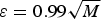
Example 1 DL level. In Section III.C, we assume that the interference number is equal to one so as to obtain a theory result. Figure 1 displays the DL level divided by maximal eigenvalue versus SIR when the interference number is greater than one. Results shows that when the input SNR is greater than the INR, the DL level  ${\varepsilon }/{\tau }$ corresponding to ${\varepsilon }\ge 0.99\sqrt {M}$ is much greater than the maximal eigenvalue λ0 of R.
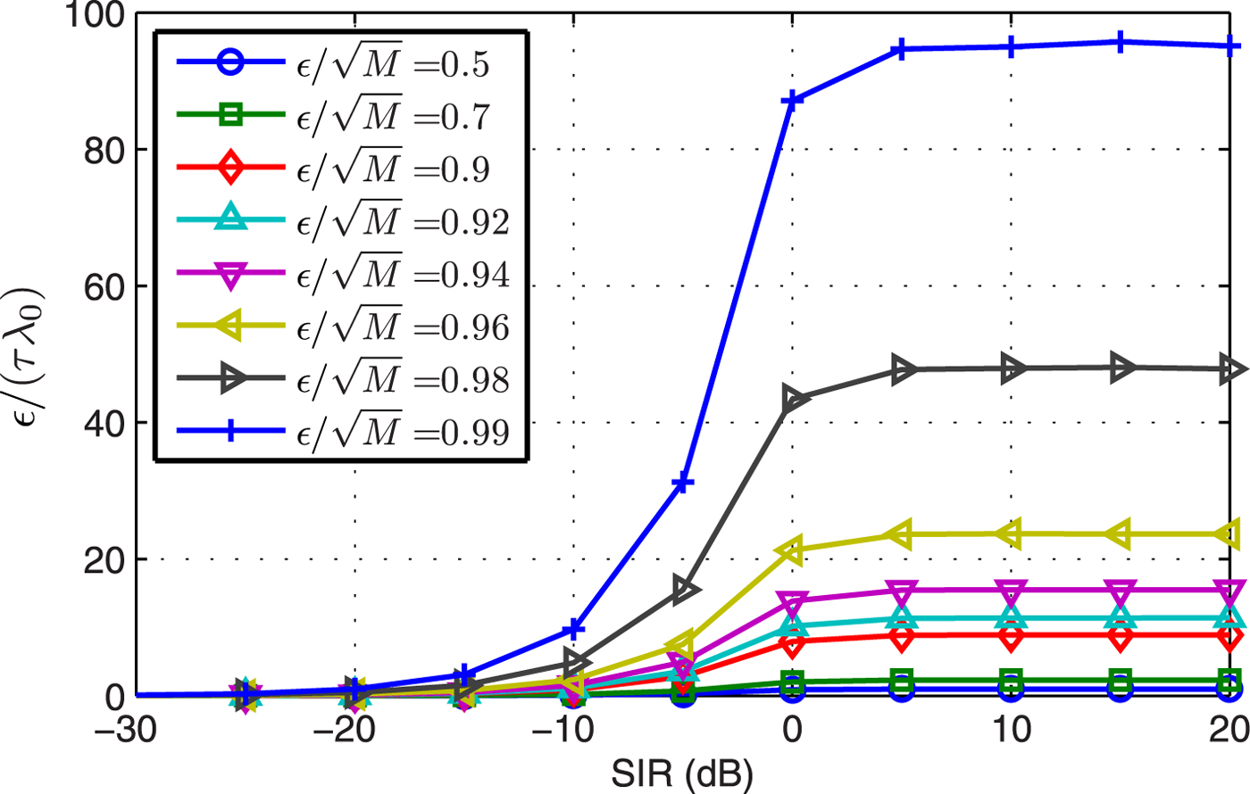
Fig. 1. The DL level divided by maximal eigenvalue versus SIR.
Example 2 Noise subspace. Figure 2 displays the error between the estimated SSV  ${{\hat {{\bf a}}}_{0}}$ and actual SSV a0 versus SNR and dimension of EN. As discussed in Remark 2, ${{\hat {{\bf a}}}_{0}}$ is set equal to $\hat {{\bf a}}({{\hat {{\theta }}}_{0}})$ at very low SNR, hence the error is reduced to about $\mathop{\min}\limits_{\varphi} \left\Vert \hat {\bf a} (\hat{\theta}_{0}) e^{j{\varphi}} - {\bf a}_{0} \right\Vert = 1.95$ at very low SNR. When the SNR is >–12 dB, which approximately equals to the noise power, ${{\hat {{\bf a}}}_{0}}$ is closer to a0 than $\hat {{\bf a}}({{\hat {{\theta }}}_{0}})$. The actual dimension of noise subspace EN is 14, when estimated dimension P EN is between 9 and 14, ${{\hat {{\bf a}}}_{0}}$ is stable, which verifies the Remark 1 is reasonable.
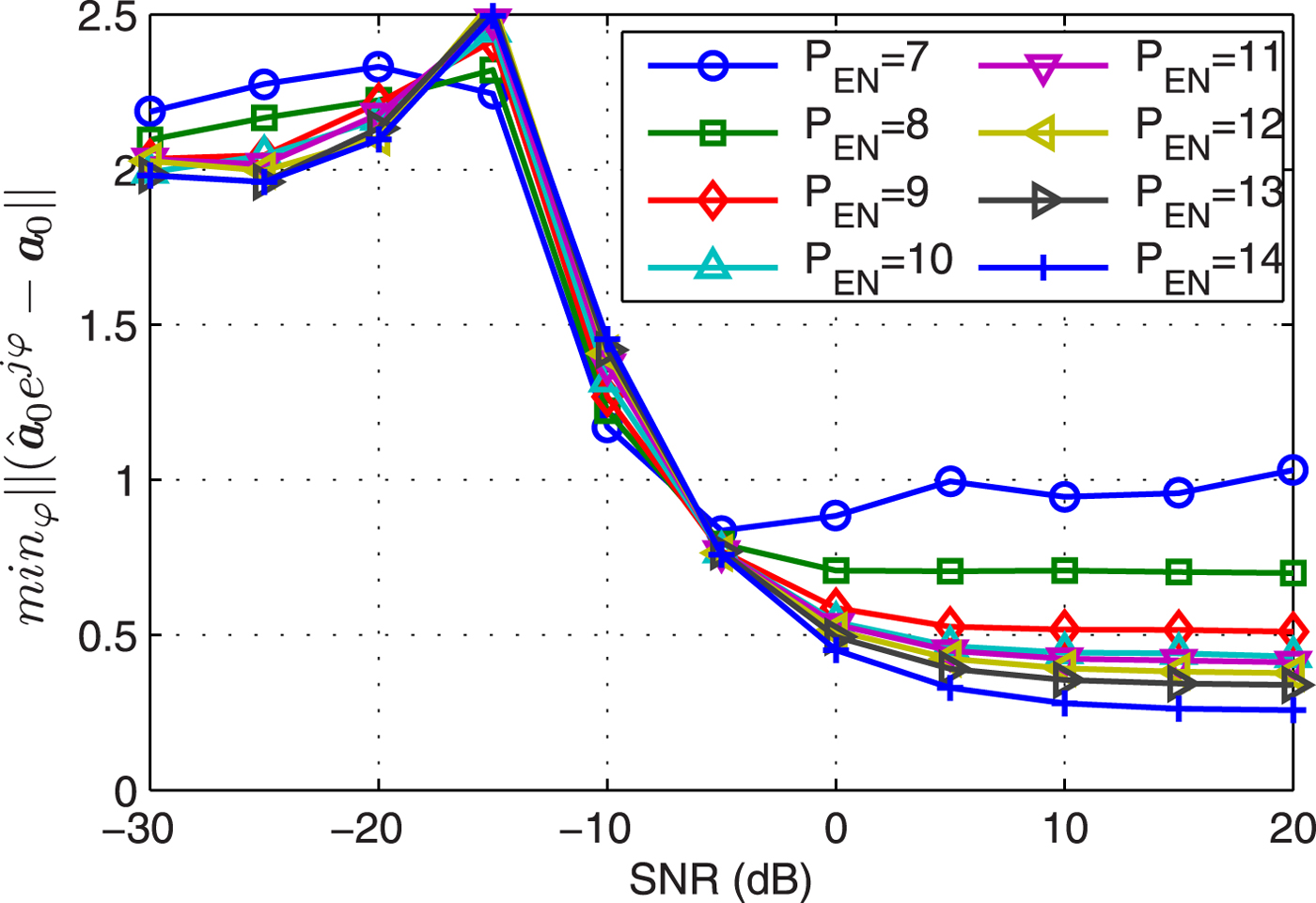
Fig. 2. The error of estimated SSV versus SNR.
Example 3 SINR versus SNR. Figure 3 displays the output SINR versus SNR with 2° pointing error. Results show that: (1) The output SINR of VDL degrades quickly when SNR is >0 dB while the SINR of FDL degrades when SNR is >10 dB, hence, the DL level with  $99\sigma _{n}^{2}$ is better than variable DL level in this case; (2) The SINR of WCB and IWCB bias from OPT when SNR is large, it is because the suppress capability of interference is decrease as the SNR gets larger. (3) The SINRs of RIN and CFRIN are close to OPT value, but a litter lower than the proposed ISRAB, the reason is analyzed in our previous work [Reference Li, Hong, Wenjun and De30]: the main peak of RIN and CFRIN cannot point to actual signal's direction even if the steering vector is accurate (also see Example 5).
Fig. 3. Output SINR versus SNR.
Example 4 SIR versus SNR. Figure 4 displays the output SIR versus SNR with 2° pointing error. Results show that: (1) The suppress capability of interference is decrease for the FDL, VDL, WCB, and IWCB when SNR is larger than 0 dB. (2) The SIR of RIN is stable through all the SNR, but a little lower than ISRAB and CFRIN especially when the SNR is very low and very high. (3) The SIR of ISRAB is higher than others expect a slight lower than the CFRCB when SNR is high.
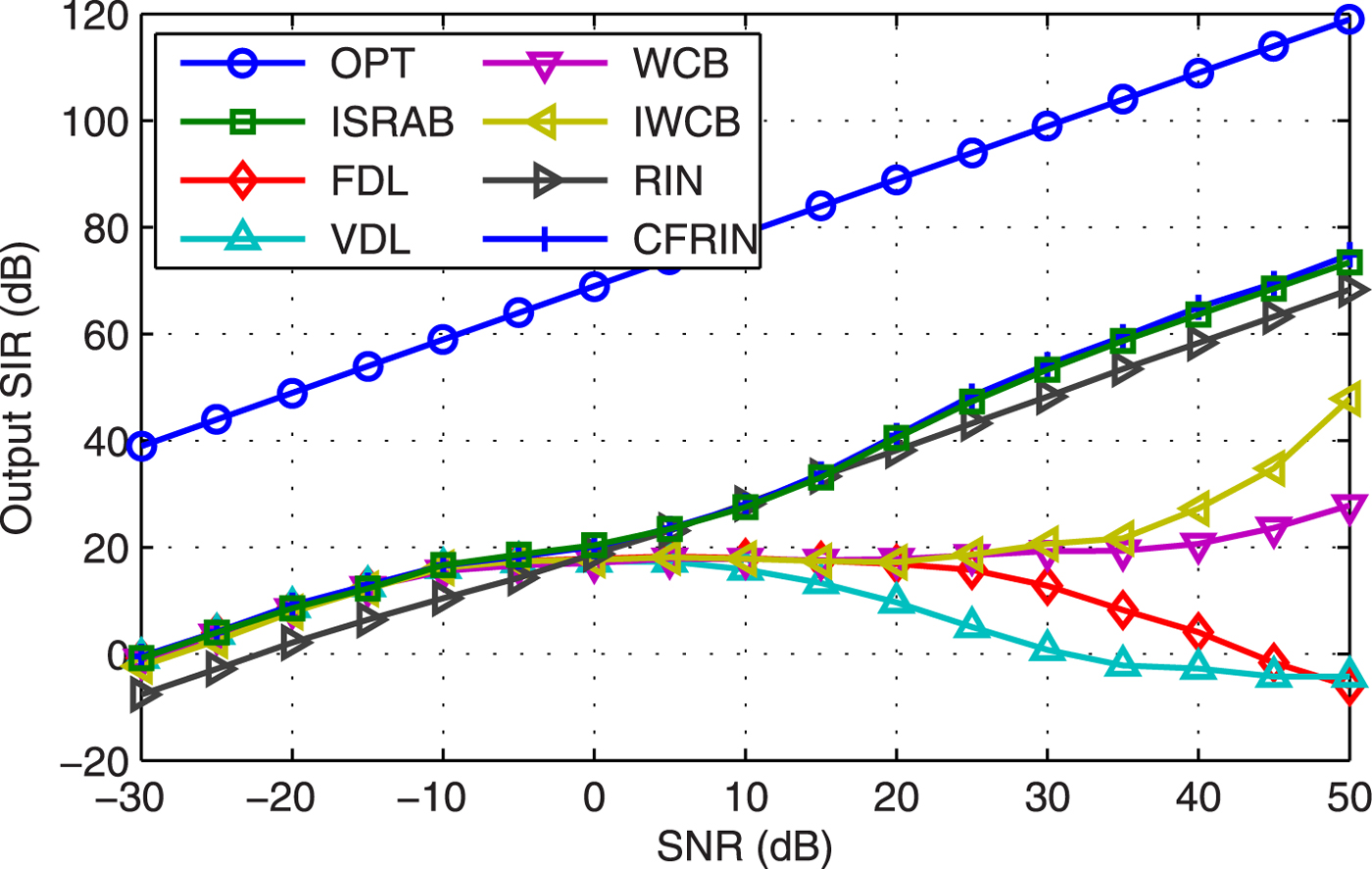
Fig. 4. Output SIR versus SNR.
Example 5 Array pattern. Figure 5 shows the array pattern of four beamformers at SNR=25 dB. Results show that: (1) Both the ISRAB and RIN form deeper nulls at interference directions than WCB. (2) The ISRAB can point the main beam peak to actual signal direction, while both the RIN and WCB deviate to the actual signal direction, even if the RIN uses actual SSV. (3) There exists self-nulling for FDL. The defect of RIN is explained as follows [Reference Li, Hong, Wenjun and De30]: the RIN in (7) contains no signal or noise component in Θ, hence the optimization condition minwHRINw in (3) has no effect in Θ. The constraint  ${{{\bf w}}^{H}}{\bf a}({\theta })=1$ guarantees that the beampattern gain is equal to one at direction ${\theta }$, but the gain at other discrete directions in Θ may exceed one without enlarging wHRINw. Then the main lobe peak of beampattern may point to another direction, thus the SINR of RIN degrades slightly. The ISRAB does not have the optimization condition minwHRINw, its weight vector equivalents to ${{\hat {{\bf a}}}_{0}}$ which is very close to actual SSV (as shown in Fig. 2), so the main beam of ISRAB can point (very close) to actual signal's directions. Because the solution of WCB is equivalent to the DL, the peak of the main beam is moved with the DL level when there exists a pointing error [Reference Wang, Wu and Liang31].
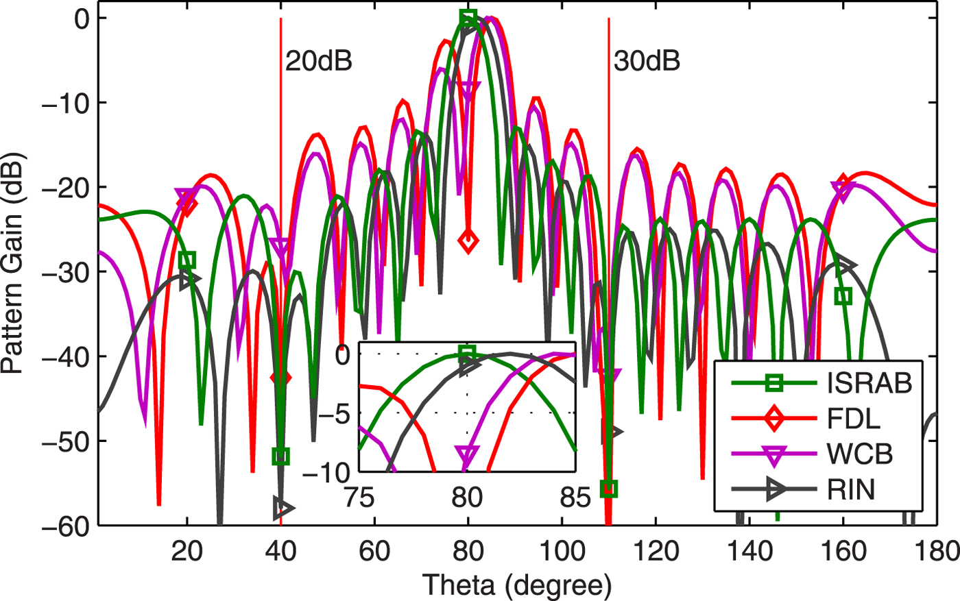
Fig. 5. Array pattern.
Example 6 Pointing error. Figure 6 displays the output SINR versus pointing error, SNR=25 dB. Results show that: (1) Whether FDL or VFL is not suitable in this scenario. (2) We set  ${\varepsilon }=2$ for WCB, which corresponds to about 2° pointing error. the SINR of WCB performs stable when pointing error is less than 2°, but degrades greatly when the pointing error is larger than 2°. (3) When the pointing error is $<{{{\theta }}_{W}}/2={\rm 4}{}^\circ $, ISRAB performs stably, and its SINR is the closest to OPT. (4) It is because the stopping criterion in Remark 2 causes the SINR of ISRAB decrease when the pointing error is larger than 4°, the CFRIN has the same stopping criterion while the RIN does not have.
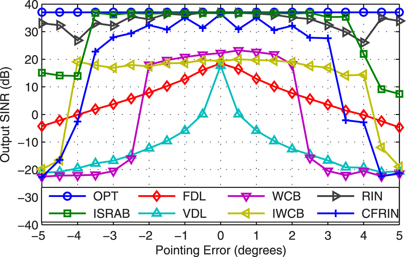
Fig. 6. Output SINR versus pointing error.
Example 7 Snapshots. Figure 7 displays the output SINR versus snapshots at  $\hbox {SNR}=25$ dB. Results shows that the performance of ISRAB tends to be stable when the number of snapshots is larger than 20. The SINR performance is not good with small snapshots is a drawback of the ISRAB, as well as the CFRIN.
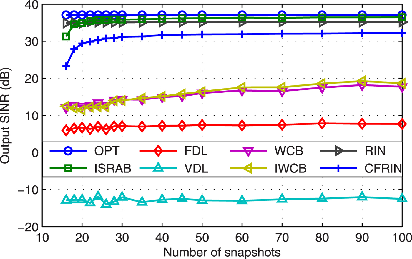
Fig. 7. Output SINR versus snapshots.
B) Array perturbations
In the following examples, the SV mismatch is caused by both 2° pointing error, and array perturbations with  ${{{\sigma }}_{\Delta }}=0.02$.
Example 8 SINR versus SNR. Figure 8 shows the output SINR versus SNR. Compared with Fig. 3, the SINR of RIN degrades with a fixed value through all the SNRs in Fig. 8. The SINR of ISRAB is very close to OPT at low SNR, although it degrades at high SNR, it is always better than other beamformers.
Fig. 8. Output SINR versus SNR.
Example 9 SIR versus SNR. Figure 9 displays the output SIR versus SNR with pointing error and array perturbations. Compared with Fig. 4, the SIRs of RIN and CFRIN are decreased at low SNR case, the SIR of ISRAB almost outperforms others through all the SNRs.
Fig. 9. Output SIR versus SNR.
Example 10 Array pattern. Figure 10 displays the array pattern at  $\hbox {SNR}=25$ dB. The ISRAB can point the main lobe peak closest to actual signal direction than RIN and WCB. Although the nulling depths at interference directions of ISRAB are lower than that of Fig. 3, they are much deeper than WCB in this scenario.
Fig. 10. Array pattern.
Finally, the main advantages of the proposed ISRAB are summarized as follows: (1) The nulling at interference is much deeper; (2) The main peak can point to signal's actual directions; (3) All the parameters are fixed in any situations.
V. CONCLUSION
A novel robust adaptive beamformer ISRAB has been developed. Three steps processing are performed to guarantee that the beamformer's weight is orthogonal to each ISV and does not suppress the desired signal as an interference. Theoretical analysis of the interference suppression principle is analyzed in detail. Some special set of parameters are also analyzed. Simulation results show that, compared with several classical beamformers, the proposed ISRAB has the advantages in many cases, such as the pointing error and array perturbations.
ACKNOWLEDGMENT
The authors wish to thank the Handling Editor and Reviewers for their detailed review, which helped improve this paper.
FINANCIAL SUPPORT
This work is supported by the scientific research foundation of Hubei Provincial Department of Education (Yang Li, grant numbers Q20181505).
STATEMENT OF INTEREST
The authors declare no conflict of interest.
Linxian Liu received the bachelor degree from Hunan Normal University in 2008 and received her master degree from South-Central University for Nationalities in 2011, respectively. She is currently a lecturer of Wuhan College of Foreign Languages and Foreign Affairs. Her main research interests are signal processing and technology English writing.
Yang Li received the B.S. degree in optical information science and technology and the M.S. degree in radio physics from Wuhan University of Technology, Wuhan, China, in 2006 and 2010, respectively, and received the Ph.D. degree in electromagnetic field and microwave technology from Huazhong University of Science and Technology, Wuhan, China, in 2016. He was with the FiberHome Technologies Group, Wuhan, in 2011, and CSIC No.722 Research and Development Institute, Wuhan, in 2016. He is currently a lecturer of School of Electrical and Information Engineering, Wuhan Institute of Technology, Wuhan, China. His research interests include array signal processing, radar signal processing, and radio wave propagation.


 Open access