


1 Introduction
Let  $(M,ds^{2})$ be a Kähler manifold of complex dimension
  $n$ with the Kähler metric
 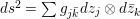 $ds^{2}=\sum g_{j\bar{k}}dz_{j}\otimes d\bar{z}_{k}$ in local coordinates. Let
  ${\it\omega}=\sqrt{-1}/2{\it\pi}\sum g_{j\bar{k}}dz_{j}\wedge d\bar{z}_{k}$ be the positive
  $(1,1)$-form associated to the Kähler metric
  $ds^{2}$, and let
  $Ric({\it\omega})=-\sqrt{-1}/2{\it\pi}\partial \bar{\partial }\log \det (g_{j\bar{k}})$ be the Ricci form of
  ${\it\omega}$. Then
  $ds^{2}$ is called Kähler–Einstein if
  $Ric({\it\omega})$ is proportional to the Kähler form
  ${\it\omega}$.
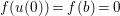
In the present paper, we focus ourselves on the explicit Kähler–Einstein metrics of certain bounded pseudoconvex domains in  $\mathbb{C}^{n}$. It is proved that for any domain of holomorphy, there is a unique complete Kähler–Einstein metric, with the Ricci curvature
  $-{\it\lambda}$, whose generating function
  $g$ satisfies the following Monge–Ampère equation with Dirichlet boundary condition:
 $$\begin{eqnarray}\displaystyle & \displaystyle \det \left(\frac{\partial ^{2}g}{\partial z_{j}\partial \overline{z}_{k}}\right)=e^{{\it\lambda}g}\quad (z\in D), & \displaystyle\end{eqnarray}$$
 $$\begin{eqnarray}\displaystyle & \displaystyle g(z)\rightarrow \infty \quad (z\rightarrow \partial D), & \displaystyle\end{eqnarray}$$
 where  $(\partial ^{2}g/\partial z_{j}\partial \overline{z}_{k})=(g_{j\bar{k}})$ (see [Reference Cheng and Yau6], [Reference Mok and Yau12], [Reference Wu and Fornaess19]).
Usually, it is difficult to solve the above nonlinear partial differential equation (1) for general bounded pseudoconvex domains in  $\mathbb{C}^{n}$. It is well known that, for any bounded homogeneous domain in
  $\mathbb{C}^{n}$, the Bergman metric has constant Ricci curvature
  $-1$ [Reference Bergman4]. Thus, the Bergman metric is identical to the Kähler–Einstein metric constructed by Cheng and Yau in [Reference Cheng and Yau6]. For nonhomogeneous cases, it was Bland who first described the Kähler–Einstein metric for the Thullen domain
  ${\rm\Omega}_{p}:=\{(z,w)\in \mathbb{C}^{n-1}\times \mathbb{C}:|w|^{2}<(1-\Vert z\Vert ^{2})^{1/p}\}$,
  $p>0$ in [Reference Bland5], where the Monge–Ampère equation was reduced to an ordinary differential equation. Later, Yin and Roos generalized the Thullen domain to Cartan–Hartogs domains (see [Reference Wang, Yin, Zhang and Zhang18] for the definition). With Wang and Zhang, they obtained the explicit Kähler–Einstein metrics for Cartan–Hartogs domains in some critical cases [Reference Wang, Yin, Zhang and Roos17, Reference Wang, Yin, Zhang and Zhang18]. In general, the Cartan–Hartogs domains are not homogeneous due to [Reference Ahn, Byun and Park1] and [Reference Roos14], where the full holomorphic automorphism groups have been described explicitly already.
One observation of the above special domains is that both of them can be regarded as certain kinds of Hartogs domains, which are based on the unit ball or, more generally, bounded symmetric domains. The right-hand side of the defining inequality for either the Thullen domain or Cartan–Hartogs domains is exactly some negative power of the Bergman kernel (up to a constant). Besides, it is well known that bounded symmetric domains are special kinds of homogeneous domains. Therefore, we consider a more general type of Hartogs domain in this paper, named the Bergman–Hartogs domain, which is based on a bounded homogeneous domain. The setting of the Bergman–Hartogs domain is as follows.
Let  $D$ be a bounded homogeneous domain in
  $\mathbb{C}^{n}$, and let
  $K_{D}(z,{\it\zeta})$ denote the Bergman kernel off the diagonal for
  $D$. Then we define the Bergman–Hartogs domain as
 $$\begin{eqnarray}\displaystyle {\rm\Omega}_{s}:=\left\{(z,z_{n+1})\in D\times \mathbb{C}:|z_{n+1}|^{2}<K_{D}(z,z)^{-s}\right\}, & & \displaystyle\end{eqnarray}$$
 where  $z=(z_{1},\ldots ,z_{n})\in D$, and
  $s$ is a positive real number.
It is known that  $D$ is Bergman exhaustive since
  $D$ is homogeneous, that is,
  $K_{D}(z,z)\rightarrow +\infty$ as
  $z\rightarrow \partial D$ (see [Reference Kobayashi9], Proposition 5.2), then
  ${\rm\Omega}_{s}$ is a bounded domain in
  $\mathbb{C}^{n+1}$. Note that
  $D$ is pseudoconvex and
  $\log K_{D}(z,z)$ is plurisubharmonic; we know that
  ${\rm\Omega}_{s}$ is a bounded pseudoconvex domain in
  $\mathbb{C}^{n+1}$(see [Reference Saitoh, Alpay, Ball and Ohsawa15, p. 142]). Consequently, there exists a unique complete Kähler–Einstein metric on
  ${\rm\Omega}_{s}$ due to Mok and Yau [Reference Mok and Yau12], and we have the following result.
Theorem 1.1. Let  ${\rm\Omega}_{s}$ be the Bergman–Hartogs domain defined as in (3). Assume that the Bergman kernel on
  $D$ satisfies
  $K_{D}(z,0)=K_{D}(0,0)$, then the generating function
  $g$ for the complete Kähler–Einstein metric of
  ${\rm\Omega}_{s_{0}}$ is given by
 $$\begin{eqnarray}\displaystyle g(z,z_{n+1})=-\!\log \left(K_{D}(z,z)^{-s_{0}}-|z_{n+1}|^{2}\right)+C, & & \displaystyle\end{eqnarray}$$
 where  $s_{0}=1/(n+1)$ and the constant
  $C$ is given by
 $$\begin{eqnarray}C=\frac{1}{n+2}\log \frac{\det T_{D}(0,0)}{(n+1)^{n}K_{D}(0,0)}.\end{eqnarray}$$
 The notations  $K_{D}(0,0)$ and
  $T_{D}(0,0)$ denote the Bergman kernel and the Bergman metric matrix of
  $D$ at the point
  $0$, respectively.
Notice that the condition for the Bergman kernel  $K_{D}(z,0)=K_{D}(0,0)$ holds true when
  $D$ is the Harish-Chandra realization of a bounded symmetric domain, especially when
  $D$ is one of the classical domains. This means that Theorem 1.1 generalizes the conclusions in [Reference Bland5] and [Reference Wang, Yin, Zhang and Roos17]. A complex domain
  $D$ whose Bergman kernel satisfies the condition
  $K_{D}(z,0)=K_{D}(0,0)$ is said to be a minimal domain with center 0 (see, e.g., [Reference Ishi and Kai8] for the definition of minimal domain). In 2010, Ishi and Kai proved that any bounded homogeneous domain is holomorphically equivalent to a minimal domain because a homogeneous representative domain is minimal [Reference Ishi and Kai8, Proposition 3.8]. As an application of the above arguments and Theorem 1.1, we have the following corollary.
Corollary 1.2. Let  ${\mathcal{U}}$ be a bounded homogeneous representative domain in
  $\mathbb{C}^{n}$, and let
  $\widehat{{\rm\Omega}}_{s}$ be the corresponding Bergman–Hartogs domain based on
  ${\mathcal{U}}$. Then the Kähler–Einstein metric for
  $\widehat{{\rm\Omega}}_{s_{0}}$ is generated by
 $$\begin{eqnarray}\displaystyle {\hat{g}}(z,z_{n+1})=-\!\log \left(K_{{\mathcal{U}}}(z,z)^{-s_{0}}-|z_{n+1}|^{2}\right)+C^{\prime }, & & \displaystyle\end{eqnarray}$$
 where  $s_{0}=1/(n+1)$, and the constant
  $C^{\prime }$ is given similarly to (4).
The authors knew the definition of the Bergman–Hartogs domain in the winter of 2012, communicated by Roos. Recently, the full holomorphic automorphism group  $\text{Aut}({\rm\Omega}_{s})$ was given by Roos in [Reference Roos14]. Therefore, we know that
  ${\rm\Omega}_{s}$ is not homogeneous in general, except for when
  ${\rm\Omega}_{s}$ is the Euclidean unit ball in
  $\mathbb{C}^{n+1}$. Park and Yamamori [Reference Park and Yamamori13] have computed the Bergman kernel for
  ${\rm\Omega}_{s}$ and considered the corresponding Lu Qikeng problem. The authors would like to thank Professor Roos for giving them the preprint [Reference Roos14] and Park for showing them the preprint [Reference Park and Yamamori13].
The paper is organized as follows. In Section 2, we give a subgroup of the holomorphic automorphism group  $\text{Aut}({\rm\Omega}_{s})$ for the Bergman–Hartogs domain
  ${\rm\Omega}_{s}$. This allows us to reduce the Monge–Ampère equation to an ordinary differential equation in Section 3, following the method used in [Reference Wang, Yin, Zhang and Roos17], where
  $D$ is one of the classical domains in the sense of Loo-Keng Hua. The reduced ordinary equation can be solved explicitly for a special value
  $s_{0}$ of the parameter
  $s$. In Section 4, we consider the minimality of bounded representative homogeneous domains introduced by Ishi and Kai in [Reference Ishi and Kai8], and give a sufficient condition for a bounded homogeneous domain to be minimal by comparing the Jacobi of the representative mapping and the automorphism transformation of the domain. Finally, we give some examples of Bergman–Hartogs domains, on which the Kähler–Einstein metrics are calculated explicitly.
2 Holomorphic automorphism subgroup
In this section, we present a holomorphic automorphism subgroup for the Bergman–Hartogs domain  ${\rm\Omega}_{s}$.
Recall that the domain  $D$ in the definition of
  ${\rm\Omega}_{s}$ is homogeneous, that is, for any two points
  $p,q\in D$, there exists
  ${\it\psi}\in \text{Aut}(D)$ such that
  ${\it\psi}(p)=q$. Without loss of generality, we may assume that
  $0\in D$. Then, for any
  $z\in D$, there exists
  ${\it\psi}\in \text{Aut}(D)$ such that
  ${\it\psi}(z)=0$.
Proposition 2.1. Let  ${\rm\Omega}_{s}$ be the Bergman–Hartogs domain in
  $\mathbb{C}^{n+1}$. Let
 $$\begin{eqnarray}G:=\{{\it\phi}={\it\phi}_{{\it\psi},{\it\theta}};{\it\psi}\in \text{Aut}(D),{\it\theta}\in \mathbb{R}\},\end{eqnarray}$$
 where  ${\it\phi}_{{\it\psi},{\it\theta}}(z,z_{n+1}):=({\it\psi}(z),(\det J_{{\it\psi}}(z))^{s}e^{\sqrt{-1}{\it\theta}}z_{n+1})$ for
  $(z,z_{n+1})\in {\rm\Omega}_{s}$, and
  $\det J_{{\it\psi}}(z)$ denotes the Jacobian of
  ${\it\psi}$ at
  $z$, then
  $G$ is a subgroup of
  $\text{Aut}({\rm\Omega}_{s})$.
It is known that any bounded homogeneous domain is simply connected [Reference Vinberg, Gindikin and Pjateckii-Šapiro16], hence one can take a branch of  $(\det J_{{\it\psi}}(z))^{s}$ to be a single-valued holomorphic function on
  $D$ since
  $\det J_{{\it\psi}}(z)$ is a nonzero holomorphic function on
  $D$, and other branches can be obtained by multiplying
  $e^{\sqrt{-1}{\it\theta}}$ by appropriate constants
  ${\it\theta}$.
Proof of Proposition 2.1.
A direct calculation shows that
 $$\begin{eqnarray}\left|\left(\det J_{{\it\psi}}(z)\right)^{s}e^{\sqrt{-1}{\it\theta}}z_{n+1}\right|^{2}K_{D}({\it\psi}(z),{\it\psi}(z))^{s}=\left|z_{n+1}\right|^{2}K_{D}(z,z)^{s},\end{eqnarray}$$
 where  $K_{D}$ denotes the Bergman kernel of the bounded homogeneous domain
  $D$. This means that
  ${\it\phi}(z,z_{n+1})\in {\rm\Omega}_{s}$ for any point
  $(z,z_{n+1})\in {\rm\Omega}_{s}$.
It is obvious that  ${\it\phi}$ is invertible and
  ${\it\phi}_{1}\circ {\it\phi}_{2}\in G$ for any
  ${\it\phi}_{1},{\it\phi}_{2}\in G$, since
  ${\it\psi}\in \text{Aut}(D)$. Therefore,
  $G$ is a subgroup of
  $\text{Aut}({\rm\Omega}_{s})$.◻
Remark 2.1. In [Reference Roos14], Roos proved that  $G=\text{Aut}({\rm\Omega}_{s})$, that is,
  $G$ is the full holomorphic automorphism group unless
  ${\rm\Omega}_{s}$ is the Euclidean unit ball. The method is almost the same as in [Reference Ahn, Byun and Park1] (see [Reference Ahn, Byun and Park1] and [Reference Roos14] for more details).
Remark 2.2. Since  $D$ is homogeneous, we know from Proposition 2.1 that for any point
  $(z,z_{n+1})\in {\rm\Omega}_{s}$, there exists
  ${\it\phi}\in G$ such that
  ${\it\phi}(z,z_{n+1})=(0,w_{n+1})$.
Now we define a  $G$-invariant function on
  ${\rm\Omega}_{s}$, which is used frequently in the following text for convenience.
Proposition 2.2. For any point  $(z,z_{n+1})\in {\rm\Omega}_{s}$, we define
 $$\begin{eqnarray}x(z,z_{n+1})=\left|z_{n+1}\right|^{2}K_{D}(z,z)^{s}.\end{eqnarray}$$
 Then  $x$ is invariant under the holomorphic automorphism subgroup
  $G$, that is,
  $x({\it\phi}(z,z_{n+1}))=x(z,z_{n+1})$ for any element
  ${\it\phi}\in G$.
Proof. This is obviously due to the formula (7).
One can immediately see that the real-valued function  $x$ takes values in the interval
  $[0,1)$ by the definition of the Bergman–Hartogs domain
  ${\rm\Omega}_{s}$.
In order to simplify the computations in Section 3, we present the Jacobian determinant of  ${\it\phi}\in G$ here.
Proposition 2.3. For  $Z=(z,z_{n+1})\in {\rm\Omega}_{s}$, the Jacobian of
  ${\it\phi}={\it\phi}_{{\it\psi},{\it\theta}}\in G$ is given by
 $$\begin{eqnarray}\left|\det J_{{\it\phi}}(Z)\right|^{2}=\left(\frac{K_{D}(z,z)}{K_{D}({\it\psi}(z),{\it\psi}(z))}\right)^{s+1},\end{eqnarray}$$
 where  ${\it\psi}\in \text{Aut}(D)$. In particular, one can choose one
  ${\it\psi}_{z}\in \text{Aut}(D)$ such that
  ${\it\psi}_{z}(z)=0$, and the Jacobian of the corresponding
  ${\it\phi}_{z}\in G$ is
 $$\begin{eqnarray}\left|\det J_{{\it\phi}_{z}}(Z)\right|^{2}=\left(\frac{K_{D}(z,z)}{K_{D}(0,0)}\right)^{s+1}.\end{eqnarray}$$
Proof. Let  $Z=(z,z_{n+1})\in {\rm\Omega}_{s}$. Because
 $$\begin{eqnarray}{\it\phi}(Z)=\left({\it\psi}(z),\left(\det J_{{\it\psi}}(z)\right)^{s}e^{\sqrt{-1}{\it\theta}}z_{n+1}\right),\end{eqnarray}$$
we have
 $$\begin{eqnarray}J_{{\it\phi}}(Z)=\left(\begin{array}{@{}cc@{}}J_{{\it\psi}}(z) & 0\\ \frac{\partial {\rm\Phi}(Z)}{\partial z} & \frac{\partial {\rm\Phi}(Z)}{\partial z_{n+1}}\end{array}\right),\end{eqnarray}$$
 where  ${\rm\Phi}(Z)=(\det J_{{\it\psi}}(z))^{s}e^{\sqrt{-1}{\it\theta}}z_{n+1}$. Thus, the conclusion (9) follows immediately from the well-known formula
 $$\begin{eqnarray}K_{D}(z,z)=K_{D}({\it\psi}(z),{\it\psi}(z))\left|\det J_{{\it\psi}}(z)\right|^{2},\end{eqnarray}$$
and
 $$\begin{eqnarray}\left|\frac{\partial {\rm\Phi}(Z)}{\partial z_{n+1}}\right|^{2}=\left|\det J_{{\it\psi}}(z)\right|^{2s}.\end{eqnarray}$$
 In particular, for any point  $Z=(z,z_{n+1})\in {\rm\Omega}_{s}$, we can choose a special
  ${\it\psi}_{z}\in \text{Aut}(D)$ such that
  ${\it\psi}_{z}(z)=0$ since
  $\text{Aut}(D)$ acts on
  $D$ transitively. Therefore, there exists a corresponding
  ${\it\phi}_{z}\in G$ satisfying
  ${\it\phi}_{z}(z,z_{n+1})=(0,w_{n+1})$, and consequently the Jacobian of
  ${\it\phi}_{z}$ is
 $$\begin{eqnarray}\left|\det J_{{\it\phi}_{z}}(Z)\right|^{2}=\left(\frac{K_{D}(z,z)}{K_{D}(0,0)}\right)^{s+1}.\square\end{eqnarray}$$
3 Reduction of the Monge–Ampère equation
In this section, by using the holomorphic automorphism subgroup  $G$, we reduce the complex Monge–Ampère equation to an ordinary differential equation with respect to the invariant function
  $x$, which was introduced in Proposition 2.2. Then we solve the ordinary differential equation when the parameter
  $s$ of the Bergman–Hartogs domain
  ${\rm\Omega}_{s}$ takes some critical value.
3.1 Reduction of the complex Monge–Ampère equation
Let  $D$ be any bounded homogeneous domain in
  $\mathbb{C}^{n}$, and let
  $K_{D}(z,z)$ denote the Bergman kernel for
  $D$. The Bergman–Hartogs domain is
 $$\begin{eqnarray}{\rm\Omega}_{s}:=\left\{Z=(z,z_{n+1})\in D\times \mathbb{C}:|z_{n+1}|^{2}<K_{D}(z,z)^{-s}\right\},\end{eqnarray}$$
 where  $z=(z_{1},\ldots ,z_{n})\in D$ and
  $s$ is a positive real number. According to the arguments before Theorem 1.1, we know that
  ${\rm\Omega}_{s}$ is bounded and pseudoconvex. Thanks to Mok and Yau [Reference Mok and Yau12], we know that the Bergman–Hartogs domain
  ${\rm\Omega}_{s}$ admits a unique complete Kähler–Einstein metric with the Ricci curvature
  $-(n+2)$, and the generating function, say
  $g$, of the complete Kähler–Einstein metric satisfies the following complex Monge–Ampère equation with Dirichlet boundary condition:
 $$\begin{eqnarray}\displaystyle & \displaystyle \det \left(\frac{\partial ^{2}g}{\partial z_{j}\partial \overline{z}_{k}}\right)=e^{(n+2)g}\quad (z,z_{n+1})\in {\rm\Omega}_{s}, & \displaystyle\end{eqnarray}$$
 $$\begin{eqnarray}\displaystyle & \displaystyle g(z,z_{n+1})\rightarrow \infty \quad (z,z_{n+1})\rightarrow \partial {\rm\Omega}_{s}. & \displaystyle\end{eqnarray}$$
 For simplicity of the notation, we write  $Z:=(z,z_{n+1})$ and the image
  ${\it\phi}(Z)=(w,w_{n+1})=:W$ for
  ${\it\phi}\in G$.
For any holomorphic automorphism transformation  ${\it\phi}\in G$,
  $W={\it\phi}(Z)$, we have
 $$\begin{eqnarray}\det \left(\frac{\partial ^{2}g(Z)}{\partial z_{j}\partial \overline{z}_{k}}\right)=\left|\det J_{{\it\phi}}(Z)\right|^{2}\det \left(\frac{\partial ^{2}g(W)}{\partial w_{j}\partial \overline{w}_{k}}\right),\end{eqnarray}$$
 where  $j,k$ run from
  $1$ to
  $n+1$. According to the Monge–Ampère equation (11), Equation (13) is equivalent to
 $$\begin{eqnarray}e^{(n+2)g(Z)}=|\text{det }J_{{\it\phi}}(Z)|^{2}e^{(n+2)g(W)}.\end{eqnarray}$$
That is,
 $$\begin{eqnarray}g(Z)=g({\it\phi}(Z))+\frac{1}{n+2}\log \left|\det J_{{\it\phi}}(Z)\right|^{2}.\end{eqnarray}$$
 Now we fix a point  $Z=(z,z_{n+1})\in {\rm\Omega}_{s}$ for a moment. As explained in the proof of Proposition 2.3, we can take a special
  ${\it\phi}_{z}\in G$ such that
 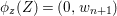 ${\it\phi}_{z}(Z)=(0,w_{n+1})$. By Proposition 2.3, we know that
 $$\begin{eqnarray}\left|\det J_{{\it\phi}_{z}}(Z)\right|^{2}=\left(\frac{K_{D}(z,z)}{K_{D}(0,0)}\right)^{s+1},\end{eqnarray}$$
then Equation (15) yields
 $$\begin{eqnarray}g(Z)=g\left(0,w_{n+1}\right)+\frac{s+1}{n+2}\log K_{D}(z,z)-\frac{s+1}{n+2}\log K_{D}(0,0).\end{eqnarray}$$
 As  $Z$ varies in
  ${\rm\Omega}_{s}$, Equation (17) holds true on
  ${\rm\Omega}_{s}$ since we can always take
  ${\it\phi}_{z}\in G$ such that
  ${\it\phi}_{z}(Z)=(0,w_{n+1})$.
To obtain  $g(Z)$ explicitly, we need to know
  $g(0,w_{n+1})$. We want to express
  $g(0,w_{n+1})$ in terms of the invariant function
  $x$, which is defined by
 $$\begin{eqnarray}x(z,z_{n+1})=\left|z_{n+1}\right|^{2}K_{D}(z,z)^{s}\end{eqnarray}$$
 in Proposition 2.2. Note that  $x$ is invariant under
  $G$, that is,
  $\forall {\it\phi}\in G,x({\it\phi}(Z))=x(Z)$, thus we have
  $x(Z)=x({\it\phi}_{z}(Z))=x(0,w_{n+1})$. It follows that
 $$\begin{eqnarray}|w_{n+1}|^{2}=xK_{D}(0,0)^{-s}.\end{eqnarray}$$
 By taking a suitable  ${\it\theta}$ in the automorphism
  ${\it\phi}_{z}$, say
  ${\it\theta}_{z}$, we can assume that
  $w_{n+1}$ is real. Therefore, one can regard
  $g(0,w_{n+1})$ as a real-valued function of the real variable
  $x$.
$x$.
Let  $y(x):=g(0,w_{n+1})$, then Equation (17) becomes
 $$\begin{eqnarray}g(Z)=y(x)+\frac{s+1}{n+2}\log K_{D}(z,z)-\frac{s+1}{n+2}\log K_{D}(0,0).\end{eqnarray}$$
 Differentiating both sides of the above equation with respect to  $Z=(z,z_{n+1})$, we have
 $$\begin{eqnarray}\displaystyle \left(\frac{\partial ^{2}g}{\partial z_{j}\partial \overline{z}_{k}}\right) & = & \displaystyle \left(\frac{\partial }{\partial Z}\right)^{t}\frac{\partial }{\partial \overline{Z}}g\nonumber\\ \displaystyle & = & \displaystyle \left(\frac{\partial }{\partial Z}\right)^{t}\frac{\partial }{\partial \overline{Z}}y+\frac{s+1}{n+2}\left(\frac{\partial }{\partial Z}\right)^{t}\frac{\partial }{\partial \overline{Z}}\log K_{D}(z,z),\end{eqnarray}$$
 where  $\partial /\partial Z=(\partial /\partial z_{1},\ldots ,\partial /\partial z_{n},\partial /\partial z_{n+1})$ and
  $(\partial /\partial Z)^{t}$ denotes the transpose of
  $\partial /\partial Z$. Notice that
 $$\begin{eqnarray}\frac{\partial y}{\partial Z}=\left(y^{\prime }\frac{\partial x}{\partial z_{1}},\ldots ,y^{\prime }\frac{\partial x}{\partial z_{n+1}}\right)=y^{\prime }\frac{\partial x}{\partial Z}\end{eqnarray}$$
and
 $$\begin{eqnarray}\left(\frac{\partial }{\partial Z}\right)^{t}\frac{\partial }{\partial \overline{Z}}y=\left(\frac{\partial }{\partial Z}\right)^{t}\left(y^{\prime }\frac{\partial x}{\partial \overline{Z}}\right)=y^{\prime \prime }\left(\frac{\partial x}{\partial Z}\right)^{t}\frac{\partial x}{\partial \overline{Z}}+y^{\prime }\left(\frac{\partial }{\partial Z}\right)^{t}\frac{\partial }{\partial \overline{Z}}x,\end{eqnarray}$$
then Equation (20) can be reformulated as
 $$\begin{eqnarray}\displaystyle \left(\frac{\partial ^{2}g}{\partial z_{j}\partial \overline{z}_{k}}\right) & = & \displaystyle y^{\prime \prime }\left(\frac{\partial x}{\partial Z}\right)^{t}\frac{\partial x}{\partial \overline{Z}}+y^{\prime }\left(\frac{\partial }{\partial Z}\right)^{t}\frac{\partial }{\partial \overline{Z}}x\nonumber\\ \displaystyle & & \displaystyle +\,\frac{s+1}{n+2}\left(\frac{\partial }{\partial Z}\right)^{t}\frac{\partial }{\partial \overline{Z}}\log K_{D}(z,z)\nonumber\\ \displaystyle & := & \displaystyle I_{1}+I_{2}+I_{3}.\end{eqnarray}$$
 Next, we want to calculate the values of  $I_{1},I_{2}$ and
  $I_{3}$ at the point
  $(0,w_{n+1})$.
Recall that
 $$\begin{eqnarray}x(z,z_{n+1})=\left|z_{n+1}\right|^{2}K_{D}(z,z)^{s},\end{eqnarray}$$
then a routine computation shows that
 $$\begin{eqnarray}\displaystyle & & \displaystyle \frac{\partial x}{\partial z_{j}}=sx\frac{\partial \log K_{D}(z,z)}{\partial z_{j}},\quad j=1,\ldots ,n;\nonumber\\ \displaystyle & & \displaystyle \frac{\partial x}{\partial z_{n+1}}=\overline{z}_{n+1}K_{D}(z,z)^{s}.\nonumber\end{eqnarray}$$
 The second-order derivatives of  $x$ give
 $$\begin{eqnarray}\displaystyle & & \displaystyle \frac{\partial ^{2}x}{\partial z_{j}\partial \overline{z}_{k}}=s^{2}x\frac{\partial \log K_{D}(z,z)}{\partial z_{j}}\frac{\partial \log K_{D}(z,z)}{\partial \overline{z}_{k}}+sx\frac{\partial ^{2}\log K_{D}(z,z)}{\partial z_{j}\partial \overline{z}_{k}},\nonumber\\ \displaystyle & & \displaystyle \frac{\partial ^{2}x}{\partial z_{j}\partial \overline{z}_{n+1}}=sz_{n+1}K_{D}(z,z)^{s}\frac{\partial \log K_{D}(z,z)}{\partial z_{j}},\nonumber\\ \displaystyle & & \displaystyle \frac{\partial ^{2}x}{\partial z_{n+1}\partial \overline{z}_{n+1}}=K_{D}(z,z)^{s},\nonumber\end{eqnarray}$$
 where  $j$ and
  $k$ run from
  $1$ to
  $n$.
$n$.
In order to get the values of the derivatives of  $x$ at the point
  $(0,w_{n+1})$, we need the following lemma.
Lemma 3.1. Let  $D$ be a bounded homogeneous domain in
  $\mathbb{C}^{n}$ containing the origin. Assume that the Bergman kernel
  $K_{D}(z,{\it\zeta})$ satisfies the condition
  $K_{D}(z,0)=K_{D}(0,0)$, then
 $$\begin{eqnarray}\frac{\partial \log K_{D}(z,z)}{\partial z}\Big|_{z=0}=\frac{\partial \log K_{D}(z,z)}{\partial \overline{z}}\Big|_{z=0}=0.\end{eqnarray}$$
Proof of the Lemma.
The conclusion follows from the fact that
 $$\begin{eqnarray}\frac{\partial K_{D}(z,z)}{\partial z}\Big|_{z=0}=\frac{\partial K_{D}(z,0)}{\partial z}\Big|_{z=0}=\frac{\partial K_{D}(0,0)}{\partial z}=0.\square\end{eqnarray}$$
Applying Lemma 3.1, we have
 $$\begin{eqnarray}\displaystyle & & \displaystyle \frac{\partial x}{\partial z_{j}}\Big|_{\left(0,w_{n+1}\right)}=sx\frac{\partial \log K_{D}(z,z)}{\partial z_{j}}\Big|_{\left(0,w_{n+1}\right)}=0,\quad j=1,\ldots ,n;\nonumber\\ \displaystyle & & \displaystyle \frac{\partial x}{\partial z_{n+1}}\Big|_{\left(0,w_{n+1}\right)}=\overline{w}_{n+1}K_{D}(0,0)^{s};\nonumber\end{eqnarray}$$
and
 $$\begin{eqnarray}\displaystyle & & \displaystyle \frac{\partial ^{2}x}{\partial z_{j}\partial \overline{z}_{k}}\Big|_{\left(0,w_{n+1}\right)}=sx\frac{\partial ^{2}\log K_{D}(z,z)}{\partial z_{j}\partial \overline{z}_{k}}\Big|_{z=0},\quad j,k=1,\ldots ,n;\nonumber\\ \displaystyle & & \displaystyle \frac{\partial ^{2}x}{\partial z_{j}\partial \overline{z}_{n+1}}\Big|_{\left(0,w_{n+1}\right)}=0;\nonumber\\ \displaystyle & & \displaystyle \frac{\partial ^{2}x}{\partial z_{n+1}\partial \overline{z}_{n+1}}\Big|_{\left(0,w_{n+1}\right)}=K_{D}(0,0)^{s}.\nonumber\end{eqnarray}$$
Hence, we have
 $$\begin{eqnarray}\displaystyle & & \displaystyle I_{1}\big|_{(0,w_{n+1})}=y^{\prime \prime }\left(\frac{\partial x}{\partial Z}\right)^{t}\frac{\partial x}{\partial \overline{Z}}\Big|_{(0,w_{n+1})}=\left(\begin{array}{@{}cc@{}}0 & 0\\ 0 & xy^{\prime \prime }K_{D}(0,0)^{s}\end{array}\right),\nonumber\\ \displaystyle & & \displaystyle I_{2}\big|_{(0,w_{n+1})}=y^{\prime }\left(\frac{\partial }{\partial Z}\right)^{t}\frac{\partial }{\partial \overline{Z}}x\Big|_{(0,w_{n+1})}=\left(\begin{array}{@{}cc@{}}sxy^{\prime }T_{D}(0,0) & 0\\ 0 & y^{\prime }K_{D}(0,0)^{s}\end{array}\right),\nonumber\\ \displaystyle & & \displaystyle I_{3}\big|_{(0,w_{n+1})}=\frac{s+1}{n+2}\left(\frac{\partial }{\partial Z}\right)^{t}\frac{\partial }{\partial \overline{Z}}\log K_{D}(z,z)\Big|_{z=0}=\frac{s+1}{n+2}\left(\begin{array}{@{}cc@{}}T_{D}(0,0) & 0\\ 0 & 0\end{array}\right),\nonumber\end{eqnarray}$$
where
 $$\begin{eqnarray}\left(\frac{\partial ^{2}\log K_{D}(z,z)}{\partial z_{j}\partial \overline{z}_{k}}\right)=:T_{D}(z,z)\end{eqnarray}$$
 is the Bergman metric on  $D$.
$D$.
Summarizing  $I_{1},I_{2}$ and
  $I_{3}$, we have
 $$\begin{eqnarray}\displaystyle \left(\frac{\partial ^{2}g}{\partial z_{j}\partial \overline{z}_{k}}\right)\Big|_{(0,w_{n+1})} & = & \displaystyle (I_{1}+I_{2}+I_{3})\big|_{(0,w_{n+1})}\nonumber\\ \displaystyle & = & \displaystyle \left(\begin{array}{@{}cc@{}}\left(sxy^{\prime }+\frac{s+1}{n+2}\right)T_{D}(0,0) & 0\\ 0 & \left(xy^{\prime \prime }+y^{\prime }\right)K_{D}(0,0)^{s}\end{array}\right).\nonumber\end{eqnarray}$$
Consequently, we have
 $$\begin{eqnarray}\displaystyle \det \left(\frac{\partial ^{2}g}{\partial z_{j}\partial \overline{z}_{k}}\right)\Big|_{(0,w_{n+1})} & = & \displaystyle \left(xy^{\prime \prime }+y^{\prime }\right)\left(xy^{\prime }+b\right)^{n}s^{n}K_{D}(0,0)^{s}\det T_{D}(0,0)\nonumber\\ \displaystyle & = & \displaystyle a\left[(xy^{\prime }+b)^{n+1}\right]^{\prime },\end{eqnarray}$$
 where  $a=s^{n}/(n+1)K_{D}(0,0)^{s}\det T_{D}(0,0)$ and
  $b=(1+1/s)/(n+2)$ are positive constants.
Considering the Monge–Ampère equation (11) at the point  $(0,w_{n+1})\in {\rm\Omega}_{s}$, that is
 $$\begin{eqnarray}\det \left(\frac{\partial ^{2}g}{\partial z_{j}\partial \overline{z}_{k}}\right)\Big|_{\left(0,w_{n+1}\right)}=e^{\left(n+2\right)g\left(0,w_{n+1}\right)},\end{eqnarray}$$
Equations (23) and (24) yield the following differential equation:
 $$\begin{eqnarray}a\left[(xy^{\prime }+b)^{n+1}\right]^{\prime }=e^{\left(n+2\right)y}.\end{eqnarray}$$
 Let  $u(x):=xy^{\prime }+b$; we summarize the above arguments by the following proposition.
Proposition 3.2. If
 $$\begin{eqnarray}g(Z)=y(x)+\frac{s+1}{n+2}\log \frac{K_{D}(z,z)}{K_{D}(0,0)}\end{eqnarray}$$
is a solution of the Monge–Ampère equation
 $$\begin{eqnarray}\displaystyle \det \left(\frac{\partial ^{2}g}{\partial z_{j}\partial \overline{z}_{k}}\right)=e^{(n+2)g} & & \displaystyle \nonumber\end{eqnarray}$$
 with the boundary condition  $g(z,z_{n+1})\rightarrow \infty$ when
  $(z,z_{n+1})\rightarrow \partial {\rm\Omega}_{s},$ then the function
  $u(x)=xy^{\prime }+b$ satisfies the differential equation
 $$\begin{eqnarray}\displaystyle a\left(u^{n+1}\right)^{\prime }=e^{\left(n+2\right)y} & & \displaystyle\end{eqnarray}$$
 with the initial condition  $u(0)=b$.
Proof. The differential equation (26) results from Equations (23) and (24). Next, we give an illustration about the boundary condition. We know that  $g(z,z_{n+1})\rightarrow \infty$
 $((z,z_{n+1})\rightarrow \partial {\rm\Omega}_{s})$ implies
  $y(x)=g(0,w_{n+1})\rightarrow \infty (x\rightarrow 1)$. From
 $$\begin{eqnarray}xy^{\prime }(x)=w_{n+1}\frac{\partial g(0,w_{n+1})}{\partial w_{n+1}},\end{eqnarray}$$
 we deduce that  $xy^{\prime }\rightarrow 0$ as
  $w_{n+1}\rightarrow 0$, or equivalently
  $xy^{\prime }\rightarrow 0$ as
  $x\rightarrow 0$.◻
3.2 Solution of the Monge–Ampère equation
In what follows, we solve the above differential equation (26) and obtain the generating function  $g$ for the complete Kähler–Einstein metric on
  ${\rm\Omega}_{s}$.
Integrating on both sides of Equation (26) with respect to  $x$, we have
 $$\begin{eqnarray}au^{n+1}=\int e^{\left(n+2\right)y}\,dx.\end{eqnarray}$$
By the formula of integration by parts, the right-hand side yields
 $$\begin{eqnarray}\displaystyle \int e^{\left(n+2\right)y}\,dx=xe^{\left(n+2\right)y}-\left(n+2\right)\int xy^{\prime }e^{\left(n+2\right)y}\,dx. & & \displaystyle\end{eqnarray}$$
By Equation (26), we have
 $$\begin{eqnarray}\displaystyle \int xy^{\prime }e^{(n+2)y}dx & = & \displaystyle a\int xy^{\prime }\left(u^{n+1}\right)^{\prime }\,dx\nonumber\\ \displaystyle & = & \displaystyle a(n+1)\int (u-b)u^{n}\,du\nonumber\\ \displaystyle & = & \displaystyle \frac{a(n+1)}{n+2}u^{n+2}-abu^{n+1}+ac,\end{eqnarray}$$
 where  $c$ is a constant.
 $$\begin{eqnarray}\displaystyle x\left(u^{n+1}\right)^{\prime }=(n+1)u^{n+2}+(1-b(n+2))u^{n+1}+c_{1}, & & \displaystyle\end{eqnarray}$$
 where  $c_{1}$ is a constant to be determined.
Taking the initial condition in Proposition 3.2 into consideration, that is,  $u(0)=b$ when
  $x=0$, we have
  $c_{1}=b^{n+1}(b-1)$.
Let
 $$\begin{eqnarray}\displaystyle f(u):=(n+1)u^{n+2}+\left(1-b(n+2)\right)u^{n+1}+b^{n+1}(b-1). & & \displaystyle\end{eqnarray}$$
We have the following facts.
(2) For
 $x=0$, it is easy to check that $f(u(0))=f(b)=0$.
(3)
$f^{\prime }(b)=(n+1)b^{n}>0$, which means that $\exists {\it\delta}>0$ such that $f(u)<0$ for $b-{\it\delta}<u<b$.


Claim: $u(x)\geqslant b$ for
  $0\leqslant x<1$.
Proof of Claim.
Otherwise, assume  $\exists x_{0}\in (0,1)$ such that
  $u(x_{0})<b$. Then, by the continuity of
  $u$ (we know this since
  $g$ is
  $C^{2}$),
  $\exists x_{1}\in (0,x_{0})$ such that
  $b-{\it\delta}<u(x_{1})<b$. Consequently, we have
  $f(u(x_{1}))<0$ by the fact
  $(3)$, which is in contradiction to the fact
  $(1)$.
Note that Equation (26) shows that the derivative of  $u^{n+1}$ is positive and tends to
  $\infty$ when
  $x\rightarrow 1$ (since
  $y(x)\rightarrow \infty$ when
  $x\rightarrow 1$). Then, combined with the above claim, we have
  $u^{\prime }>0$. Therefore, the function
  $u$ is strictly increasing and maps
  $[0,1)$ onto
  $[b,+\infty )$.
In summary, we have the following proposition.
Proposition 3.3. Assume that
 $$\begin{eqnarray}g(Z)=y(x)+\frac{s+1}{n+2}\log \frac{K_{D}(z,z)}{K_{D}(0,0)}\end{eqnarray}$$
 is a solution of the Monge–Ampère equation (11) with Dirichlet boundary condition, then the function  $u(x)=xy^{\prime }+b$ is the solution of the following ordinary differential equation (ODE):
 $$\begin{eqnarray}\displaystyle x\left(u^{n+1}\right)^{\prime }=f(u), & & \displaystyle\end{eqnarray}$$
 $$\begin{eqnarray}\displaystyle u\rightarrow \infty \quad \text{as}\quad x\rightarrow 1, & & \displaystyle\end{eqnarray}$$
 where  $f(u)$ is defined by (31).
Now suppose that  $u$ satisfies the ODE (32) with the boundary condition. From the above arguments, we know that
  $f(u)$ is positive on
  $(b,\infty )$, the function
  $u:[0,1)\rightarrow [b,\infty )$ is monotone and its inverse function satisfies the differential equation
 $$\begin{eqnarray}\displaystyle \frac{1}{x}\frac{dx}{du}=\frac{(n+1)u^{n}}{f(u)}, & & \displaystyle\end{eqnarray}$$
 $$\begin{eqnarray}\displaystyle x\rightarrow 1\quad \text{as}\quad u\rightarrow \infty . & & \displaystyle\end{eqnarray}$$
The solution of this equation is given by
 $$\begin{eqnarray}\displaystyle -\!\log x=\int _{u}^{\infty }\frac{(n+1)v^{n}}{f(v)}\,dv, & & \displaystyle\end{eqnarray}$$
 which gives  $x$ as a function of
  $u$, and
  $u$ as an implicit function of
  $x$. In general, it is difficult to get the explicit
  $u$. In the next subsection, we prove that when the parameter
  $s$ takes some special value then we can solve (32) with the boundary condition (32).
3.3 The critical exponent
Letting  $b=1$, that is,
  $s=1/(n+1)$ in Equation (32), we have
 $$\begin{eqnarray}\displaystyle & xu^{\prime }=u^{2}-u, & \displaystyle\end{eqnarray}$$
 $$\begin{eqnarray}\displaystyle & u\rightarrow \infty ,\quad (x\rightarrow 1). & \displaystyle\end{eqnarray}$$
The solution of the ODE (37) is
 $$\begin{eqnarray}u=\frac{1}{1-c_{2}x},\end{eqnarray}$$
 where  $c_{2}$ is an arbitrary constant to be determined.
Since  $u\rightarrow \infty$ when
  $x\rightarrow 1$, then
  $c_{2}$ has to be
  $1$. Substituting the unique solution (39) into Equation (25), we have
 $$\begin{eqnarray}\displaystyle g\left(0,w_{n+1}\right) & = & \displaystyle \frac{1}{n+2}\log \left[a(u^{n+1})^{\prime }\right]\nonumber\\ \displaystyle & = & \displaystyle -\!\log (1-x)+\frac{1}{n+2}\log (n+1)a,\nonumber\end{eqnarray}$$
 where the constant  $a=(n+1)^{-(n+1)}K_{D}(0,0)^{s_{0}}\det T_{D}(0,0)$ as in Equation (23). According to Equation (19), we have
 $$\begin{eqnarray}\displaystyle g(Z)=-\!\log (1-x)+\frac{1}{n+1}\log K_{D}(z,z)+C, & & \displaystyle \nonumber\end{eqnarray}$$
 where  $C$ is a constant defined as
 $$\begin{eqnarray}C=\frac{1}{n+2}\log \frac{\det T_{D}(0,0)}{(n+1)^{n}K_{D}(0,0)}.\end{eqnarray}$$
We claim that
 $$\begin{eqnarray}\displaystyle g(Z) & = & \displaystyle -\!\log (1-x)+\frac{1}{n+1}\log K_{D}(z,z)+C\nonumber\\ \displaystyle & = & \displaystyle -\!\log \left(K_{D}(z,z)^{-s_{0}}-|z_{n+1}|^{2}\right)+C\end{eqnarray}$$
 is the solution of the complex Monge–Ampère equation (11) with the boundary value condition on  ${\rm\Omega}_{s_{0}}$, where
  $s_{0}=1/(n+1)$.
Proof. First,  $g$ solves the complex Monge–Ampère equation (11) since the generating function
  $g$ for the Kähler–Einstein metric on
  ${\rm\Omega}_{s_{0}}$ is a solution of the ODE (32) due to Proposition 3.3, while
  $u=(1-x)^{-1}$ is the unique solution of (32) with the boundary condition. (Of course, one can also check directly that
  $g$ satisfies the Monge–Ampère equation (11).) Now we need only to check that
  $g$ satisfies the boundary value condition, that is,
  $g\rightarrow \infty$ as
 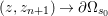 $(z,z_{n+1})\rightarrow \partial {\rm\Omega}_{s_{0}}$.
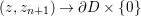
(1) When
$(z,z_{n+1})$ goes to the strongly pseudoconvex boundary points $\{(z,z_{n+1})\in D\times \mathbb{C}:|z_{n+1}|^{2}=K_{D}(z,z)^{-s_{0}},~z_{n+1}\neq 0\}$, we know that $(z,z_{n+1})\rightarrow \partial {\rm\Omega}_{s_{0}}$ implies $x\rightarrow 1$. Obviously, $g\rightarrow \infty$ as $x\rightarrow 1$.(2) When
$(z,z_{n+1})$ approaches the weakly pseudoconvex boundary points $\partial D\times \{0\}$, we have $x\rightarrow 0$. In this case, the Bergman kernel $K_{D}(z,z)$ of the bounded homogeneous domain $D$ blows up as $z\rightarrow \partial D$. Therefore, we still have $g\rightarrow \infty$ when $(z,z_{n+1})\rightarrow \partial D\times \{0\}$.


Now we can say that
 $$\begin{eqnarray}\displaystyle g(Z)=-\!\log (K_{D}(z,z)^{-s_{0}}-|z_{n+1}|^{2})+C & & \displaystyle\end{eqnarray}$$
 solves the complex Monge–Ampère equation with Dirichlet boundary value problem on  ${\rm\Omega}_{s_{0}}$, where
 $$\begin{eqnarray}C=\frac{1}{n+2}\log \frac{\det T_{D}(0,0)}{(n+1)^{n}K_{D}(0,0)}.\end{eqnarray}$$
 We call  $s_{0}=1/(n+1)$ the critical exponent. The corresponding Kähler form of the unique complete Kähler–Einstein metric on
  ${\rm\Omega}_{s_{0}}$ is given by
 $$\begin{eqnarray}\partial \bar{\partial }g=-\partial \bar{\partial }\log (K_{D}(z,z)^{-s_{0}}-|z_{n+1}|^{2}),\end{eqnarray}$$
and we conclude the proof of Theorem 1.1. ◻
4 The homogeneous domains with $K(z,0)=K(0,0)$

In this section, we turn back and take a look at the condition  $K_{D}(z,0)=K_{D}(0,0)$ for the Bergman kernel
  $K_{D}(z,{\it\zeta})$ in Theorem 1.1.
The condition  $K_{D}(z,0)=K_{D}(0,0)$ holds true when
  $D$ is the Harish-Chandra realization of a bounded symmetric domain, especially when
  $D$ is one of the classical domains. In this case, the Bergman kernels were obtained by Hua [Reference Hua7] explicitly and one can verify the above condition directly.
In general, we do not always know whether this condition does hold for homogeneous domains in  $\mathbb{C}^{n}$. Ishi and Kai [Reference Ishi and Kai8, Proposition 3.8] proved that when
  $D$ is a representative bounded homogeneous domain (see Section 4.1 for the definition of representative domains) in
  $\mathbb{C}^{n}$, one has
  $K_{D}(z,0)=K_{D}(0,0)$. Before the statement of the corollary, let us recall the definition of the representative domain.
4.1 Representative domains
The representative domain of a bounded domain  $D\subset \mathbb{C}^{n}$ was introduced by Bergman in [Reference Bergman3]. Let
  $K_{D}(z,{\it\zeta})$ denote the Bergman kernel of
  $D$. If
  $K_{D}(z,{\it\zeta})\neq 0$, then the Bergman representative mapping
  ${\it\rho}_{p}:D\rightarrow \mathbb{C}^{n}$ for a fixed point
  $p\in D$ is defined by
 $$\begin{eqnarray}{\it\rho}_{p}(z):=\frac{\partial }{\partial \overline{{\it\zeta}}^{t}}\log \frac{K_{D}(z,{\it\zeta})}{K_{D}(p,{\it\zeta})}\Big|_{{\it\zeta}=p}T_{D}(p,p)^{-1},\end{eqnarray}$$
 where  $\frac{\partial }{\partial \overline{{\it\zeta}}^{t}}=(\frac{\partial }{\partial \overline{{\it\zeta}}_{1}},\ldots ,\frac{\partial }{\partial \overline{{\it\zeta}}_{n}})^{t}$, and
  $T_{D}(z,{\it\zeta}):=(\frac{\partial ^{2}}{\partial z_{j}\partial \overline{{\it\zeta}}_{k}}\log K_{D}(z,{\it\zeta}))$ is an
  $n\times n$ complex matrix. The image
  ${\it\rho}_{p}(D)$ is called the representative domain of the bounded domain
  $D$. If
  ${\it\rho}_{p}$ is one-to-one, then the image
  ${\it\rho}_{p}(D)$, say
  ${\mathcal{U}}$, is indeed a domain.
In general, Lu [Reference Lu10] pointed out that  ${\it\rho}_{p}$ is not necessarily globally defined. Following this idea, he gave an alternative definition of the representative domain. A bounded domain
  ${\mathcal{U}}$ is called a representative domain if there is a point
  $p\in {\mathcal{U}}$ such that the Bergman metric matrix
  $T_{{\mathcal{U}}}(z,p)$ is independent of
  $z$. The point
  $p$ is called the center of the representative domain
  ${\mathcal{U}}$. For example, the Harish-Chandra realization of an irreducible bounded symmetric domain is a representative domain (up to a constant multiple). Any bounded circular domain with origin as the center is a representative domain with center
  $0$. Recently, Yamamori proved that a normal quasi-circular domain in
  $\mathbb{C}^{2}$ is a representative domain with the center at the origin (see [Reference Yamamori21, Proposition 3.2] and the definition of normal quasi-circular domains therein).
4.2 Minimal domains
Let  $D$ denote a domain in
  $\mathbb{C}^{n}$ with finite volume, and fix
  $p\in D$. We say that
  $D$ is a minimal domain with a center
  $p$ if for every biholomorphism
  ${\rm\Psi}:D\simeq \tilde{D}$ with
  $\det J_{{\rm\Psi}}(p)=1$, we have
  $vol(\tilde{D})\geqslant vol(D)$, where
  $vol(D)$ denotes the Euclidean volume of
  $D$, and
  $J_{{\rm\Psi}}(p)$ denotes the Jacobian matrix of
  ${\rm\Psi}$ at
  $p$.
$p$.
Theorem 4.1. [Reference Maschler11, Theorem 3.1]
Let  $D\subset \mathbb{C}^{n}$ be a bounded univalent domain and
  $p\in D$. Then
  $D$ is a minimal domain with a center
  $p$ if and only if
  $K_{D}(z,p)(z\in D)$ is constant on
  $D$.
$D$.
In general, Maschler [Reference Maschler11] proved that a representative domain is not necessarily minimal. Fortunately, for bounded homogeneous domains, Ishi and Kai [Reference Ishi and Kai8] proved the following theorem.
Corollary 4.2. [Reference Ishi and Kai8, Corollary 3.8]
The representative domain  ${\mathcal{U}}$ of a bounded homogeneous domain
  $D\in \mathbb{C}^{n}$ is minimal with a center
  $0$.
$0$.
Therefore, combined with Theorem 1.1 and Corollary 4.2, we have the following corollary.
Corollary 4.3. Assume that  ${\mathcal{U}}$ is the representative domain of a bounded homogeneous domain
  $D\subset \mathbb{C}^{n}$. Let
  $\widehat{{\rm\Omega}}_{s}$ be the corresponding Bergman–Hartogs domain built on
  ${\mathcal{U}}$. Then the Kähler–Einstein metric for
  $\widehat{{\rm\Omega}}_{s_{0}}$ is generated by
 $$\begin{eqnarray}\displaystyle {\hat{g}}(z,z_{n+1})=-\!\log \!\left(K_{{\mathcal{U}}}(z,z)^{-s_{0}}-|z_{n+1}|^{2}\right)+C, & & \displaystyle\end{eqnarray}$$
 where  $s_{0}=1/n+1$, and
  $C$ is a constant as in (40).
For general bounded domains in  $\mathbb{C}^{n}$, even for homogeneous domains, we cannot expect
  $K_{D}(z,0)=K_{D}(0,0)$ any more. It was pointed out by the referee that
  $K_{D}(z,0)=K_{D}(0,0)$ is actually equivalent to the domain
  $D$ being minimal with the center
  $0$. The authors are grateful to the referee for interpreting the following example. A simply connected domain
  ${\rm\Omega}\subset \mathbb{C}$ is symmetric because it is biholomorphic to the unit disc
  ${\rm\Delta}$ by the Riemann mapping theorem, while
  ${\rm\Omega}$ is minimal with some center only if
  ${\rm\Omega}$ is the image of
  ${\rm\Delta}$ by an affine map
  $z\mapsto az+b$, thanks to [Reference Ishi and Kai8, Proposition 3.4]. Indeed, the minimality and the representativeness of
  ${\rm\Omega}$ are equivalent in this case. Hence, there exist many bounded symmetric domains whose Bergman kernels do not satisfy the condition
  $K_{D}(z,0)=K_{D}(0,0)$.
4.3 A sufficient condition for $K_{D}(z,0)=K_{D}(0,0)$

From the above arguments, we know that the minimality of a bounded domain is not an intrinsic property, that is, it is not biholomorphically invariant. Therefore the Bergman kernel condition  $K_{D}(z,0)=K_{D}(0,0)$ does not always hold even for homogeneous domains. In the following, we give a sufficient condition such that
  $K_{D}(z,0)=K_{D}(0,0)$ holds for all bounded homogeneous domains
  $D$ in
  $\mathbb{C}^{n}$.
Proposition 4.4. Let  $D$ be a bounded homogeneous domain in
  $\mathbb{C}^{n}$ and
  $0\in D$. Let
  ${\mathcal{U}}:={\it\rho}_{p}(D)$ be the representative domain of
  $D$. Take
  ${\it\psi}_{p}\in \text{Aut}(D)$ satisfying
  ${\it\psi}_{p}(p)=0$, then
  $K_{D}(z,0)=K_{D}(0,0)$ if
 $$\begin{eqnarray}\det J_{{\it\rho}_{p}}(z)=\frac{\det J_{{\it\psi}_{p}}(z)}{\det J_{{\it\psi}_{p}}(p)},\end{eqnarray}$$
 where  $\det J_{{\it\psi}}(z)$ denotes the determinant of the Jacobian matrix of
  ${\it\psi}$ at
  $z$.
$z$.
Proof. Under the assumptions in the proposition, it is well known that
 $$\begin{eqnarray}\displaystyle K_{D}(z,p)=K_{{\mathcal{U}}}({\it\rho}_{p}(z),0)\det J_{{\it\rho}_{p}}(z)\det \overline{J_{{\it\rho}_{p}}(p)},\quad z\in D; & & \displaystyle\end{eqnarray}$$
 $$\begin{eqnarray}\displaystyle K_{D}(z,p)=K_{D}({\it\psi}_{p}(z),0)\det J_{{\it\psi}_{p}}(z)\det \overline{J_{{\it\psi}_{p}}(p)},\quad z\in D. & & \displaystyle\end{eqnarray}$$
 Noting that  $J_{{\it\rho}_{p}}(p)=I_{n}$, it follows that
 $$\begin{eqnarray}\frac{K_{{\mathcal{U}}}({\it\rho}_{p}(z),0)}{K_{D}({\it\psi}_{p}(z),0)}=\frac{\det J_{{\it\psi}_{p}}(z)\det \overline{J_{{\it\psi}_{p}}(p)}}{\det J_{{\it\rho}_{p}}(z)}.\end{eqnarray}$$
 Let  $z=p$ in (48), then we have
 $$\begin{eqnarray}\frac{K_{{\mathcal{U}}}(0,0)}{K_{D}(0,0)}=\frac{\left|\det J_{{\it\psi}_{p}}(p)\right|^{2}}{\left|\det J_{{\it\rho}_{p}}(p)\right|^{2}}=\left|\det J_{{\it\psi}_{p}}(p)\right|^{2}.\end{eqnarray}$$
By Proposition 4.2, we know that
 $$\begin{eqnarray}K_{{\mathcal{U}}}({\it\rho}_{p}(z),0)=K_{{\mathcal{U}}}(0,0).\end{eqnarray}$$
 Then (48) and (49) imply that  $K_{D}({\it\psi}_{p}(z),0)=K_{D}(0,0)$ if and only if
 $$\begin{eqnarray}\det J_{{\it\rho}_{p}}(z)=\frac{\det J_{{\it\psi}_{p}}(z)}{\det J_{{\it\psi}_{p}}(p)}.\end{eqnarray}$$
This completes the proof. ◻
5 Applications of the main theorem
In this section, we give some examples of Bergman–Hartogs domains.
We first investigate the relation between two generating functions of the complete Kähler–Einstein metrics on two holomorphically equivalent domains. More precisely, let  ${\rm\Phi}:{\rm\Omega}_{1}\simeq {\rm\Omega}_{2}$ be the biholomorphic mapping between two bounded pseudoconvex domains
  ${\rm\Omega}_{1}$ and
  ${\rm\Omega}_{2}$ in
  $\mathbb{C}^{n+1}$. Assume that
  $g_{1}$ and
  $g_{2}$ generate the complete Kähler–Einstein metrics on
  ${\rm\Omega}_{1}$ and
  ${\rm\Omega}_{2}$, respectively, then it follows that
 $$\begin{eqnarray}\det \left(\frac{\partial ^{2}g_{1}}{\partial z_{j}\partial \overline{z}_{k}}\right)=\left|\det J_{{\rm\Phi}}(z)\right|^{2}\det \left(\frac{\partial ^{2}g_{2}}{\partial w_{j}\partial \overline{w}_{k}}\right).\end{eqnarray}$$
 Since  $g_{1}$ and
  $g_{2}$ satisfy the Monge–Ampère equations (11) on
  ${\rm\Omega}_{1}$ and
  ${\rm\Omega}_{2}$, respectively, we have
 $$\begin{eqnarray}e^{(n+2)g_{1}}=|\text{det }J_{{\rm\Phi}}(z)|^{2}e^{(n+2)g_{2}},\end{eqnarray}$$
which yields
 $$\begin{eqnarray}g_{1}=g_{2}+\frac{1}{n+2}\log \!\left|\det J_{{\rm\Phi}}(z)\right|^{2}.\end{eqnarray}$$
5.1 Bergman–Hartogs domains over the unit ball
Denote by  $B^{n}$ the unit ball in
  $\mathbb{C}^{n}$. The Bergman–Hartogs domain over
  $B^{n}$ is
 $$\begin{eqnarray}{\rm\Omega}_{s}^{B^{n}}:=\left\{(z,z_{n+1})\in B^{n}\times \mathbb{C}:|z_{n+1}|^{2}<K_{B^{n}}(z,z)^{-s}\right\},\end{eqnarray}$$
 where  $K_{B^{n}}(z,z)=(n!/{\it\pi}^{n})1/(1-\Vert z\Vert ^{2})^{n+1}$ is the Bergman kernel of the unit ball
  $B^{n}$. When
  $s_{0}=1/(n+1)$, we get the generating function of the complete Kähler–Einstein metric by Theorem 1.1 (see also (40)) as
 $$\begin{eqnarray}\displaystyle g(z,z_{n+1}) & = & \displaystyle -\!\log \left(K_{B^{n}}(z,z)^{-s_{0}}-|z_{n+1}|^{2}\right)+C\nonumber\\ \displaystyle & = & \displaystyle -\!\log \left(({\it\pi}^{n}/n!)^{s_{0}}(1-\Vert z\Vert ^{2})-|z_{n+1}|^{2}\right)+C,\end{eqnarray}$$
 where  $C=-\!\log (n!/{\it\pi}^{n})/(n+2).$
Notice that at the moment  ${\rm\Omega}_{s_{0}}$ is biholomorphic to the unit ball
  $B^{n+1}\subset \mathbb{C}^{n+1}$ via the following map:
 $$\begin{eqnarray}\displaystyle & & \displaystyle \tilde{z}_{k}=z_{k},\quad k=1,\ldots ,n;\nonumber\\ \displaystyle & & \displaystyle \tilde{z}_{n+1}=(n!/{\it\pi}^{n})^{s_{0}/2}z_{n+1}.\nonumber\end{eqnarray}$$
 Hence, by the formula (52), the solution (53) actually gives the Kähler–Einstein metric of the unit ball  $B^{n+1}$, that is
 $$\begin{eqnarray}\displaystyle \tilde{g}(\tilde{z},\tilde{z}_{n+1})=-\!\log \left(1-\Vert \tilde{z}\Vert ^{2}-|\tilde{z}_{n+1}|^{2}\right), & & \displaystyle \nonumber\end{eqnarray}$$
 which is exactly the Bergman metric of  $B^{n+1}$ up to a factor
  $1/(n+2)$.
5.2 Bergman–Hartogs domains over bounded symmetric domains
Let  $R_{A}\;(A=I,II,III,IV)$ denote the Harish-Chandra realization of bounded symmetric domains. We take, for example, the first type
 $$\begin{eqnarray}R_{I}(p,q):=\left\{Z=(z_{jk}):I-Z\bar{Z}^{t}>0,\text{where }Z\text{ is a }p\times q\text{ matrix}\right\}\quad (p\leqslant q),\end{eqnarray}$$
 where  $I$ is the identity matrix of order
  $p$,
$p$,  $\bar{Z}$ denotes the conjugate matrix of
  $Z$, and
  $Z^{t}$ denotes the transposed matrix of
  $Z$.
$Z$.
The corresponding Bergman–Hartogs domain is defined as
 $$\begin{eqnarray}{\rm\Omega}_{s}^{R_{I}}:=\left\{(Z,W)\in R_{I}\times \mathbb{C}:|W|^{2}<K_{R_{I}}(Z,Z)^{-s}\right\},\end{eqnarray}$$
 where the Bergman kernel  $K_{R_{I}}(Z,Z)$ is [Reference Hua7]
 $$\begin{eqnarray}K_{R_{I}}(Z,Z)=\text{vol}(R_{I})^{-1}\det (I-Z\bar{Z}^{t})^{-(p+q)},\end{eqnarray}$$
 and  $vol(R_{I})$ is the volume of
  $R_{I}$. According to Theorem 1.1, when the parameter
  $s$ takes the critical value
  $1/(pq+1)$, the generating function of the complete Kähler–Einstein metric is given by
 $$\begin{eqnarray}\displaystyle g(Z,W) & = & \displaystyle -\!\log \left(K_{R_{I}}(Z,Z)^{-1/(pq+1)}-|W|^{2}\right)+C\nonumber\\ \displaystyle & = & \displaystyle -\!\log \left(\det (I-Z\bar{Z}^{t})^{(p+q)/(pq+1)}-|W|^{2}\right)+\widetilde{C},\end{eqnarray}$$
 which coincides with the Kähler–Einstein metric of the Cartan–Hartogs domain of the first type (see [Reference Wang, Yin, Zhang and Zhang18, page 47]). We omit  $R_{II},R_{III}$ and
  $R_{IV}$ here since the conclusions are almost the same.
5.3 Bergman–Hartogs domains over a nonsymmetric bounded homogeneous domain
In this subsection, we consider the Bergman–Hartogs domains over a nonsymmetric bounded minimal homogeneous domain  ${\mathcal{U}}$. It was Yamaji who observed this kind of
  ${\mathcal{U}}$ (see [Reference Yamaji20, Section 7.2]) when he considered the compactness of composition operators on the weighted Bergman space of a minimal bounded homogeneous domain.
Let  $T_{V}:=\mathbb{R}^{5}+iV$ be the tube domain over the Vinberg cone
  $V$(see [Reference Békollé and Nana2]), where
 $$\begin{eqnarray}V:=\left\{x\in \mathbb{R}^{5}:Q_{j}(x)>0,j=1,2,3\right\}\end{eqnarray}$$
and
 $$\begin{eqnarray}Q_{1}(x):=x_{1},\qquad Q_{2}(x):=x_{2}-\frac{x_{4}^{2}}{x_{1}},\qquad Q_{3}(x):=x_{3}-\frac{x_{5}^{2}}{x_{1}}.\end{eqnarray}$$
 Let  ${\mathcal{U}}$ be the representative domain of the tube
  $T_{V}$. Then
  ${\mathcal{U}}$ is a nonsymmetric minimal bounded homogeneous domain with center 0 by Proposition 4.2.
For  $z:=(z_{1},z_{2},\ldots ,z_{5})\in T_{V}$, let
 $$\begin{eqnarray}z_{[1]}:=\left(\begin{array}{@{}cc@{}}z_{1} & z_{4}\\ z_{4} & z_{2}\end{array}\right)\quad \text{and}\quad z_{[2]}=\left(\begin{array}{@{}cc@{}}z_{1} & z_{5}\\ z_{5} & z_{3}\end{array}\right)\in \text{Sym}(2,\mathbb{C}).\end{eqnarray}$$
 Then the Bergman kernel for  ${\mathcal{U}}$ on the diagonal was given by Yamaji in [Reference Yamaji20], that is,
 $$\begin{eqnarray}\displaystyle K_{{\mathcal{U}}}({\it\sigma}(z),{\it\sigma}(z)) & = & \displaystyle \frac{1}{vol({\mathcal{U}})}\left(1-{\mathcal{L}}_{1}(z_{1})\overline{{\mathcal{L}}_{1}(z_{1})}\right)^{2}\nonumber\\ \displaystyle & & \displaystyle \times \,\mathop{\prod }_{j=1}^{2}\left(\det (I-{\mathcal{L}}_{2}(z_{[j]})\overline{{\mathcal{L}}_{2}(z_{[j]})})\right)^{-3},\nonumber\end{eqnarray}$$
 where  ${\it\sigma}$ is the Bergman mapping from
  $T_{V}$ to
  ${\mathcal{U}}$ at
  $p_{0}:=(i,i,i,0,0)$, and
  ${\mathcal{L}}_{m}\;(m=1,2)$ denotes the Cayley transform
  ${\mathcal{L}}_{m}(Z):=(Z-iI_{m})$
 $(Z+iI_{m})^{-1}$ for
  $Z\in \text{Mat}(m,\mathbb{C})$.
The corresponding Bergman–Hartogs domains over the nonsymmetric homogeneous domain  ${\mathcal{U}}$ are defined as
 $$\begin{eqnarray}{\rm\Omega}_{s}^{{\mathcal{U}}}:=\left\{({\it\xi},{\it\xi}_{6})\in {\mathcal{U}}\times \mathbb{C}:|{\it\xi}_{6}|^{2}<K_{{\mathcal{U}}}({\it\xi},{\it\xi})^{-s}\right\},\end{eqnarray}$$
 where  ${\it\xi}:={\it\sigma}(z)\in {\mathcal{U}}$. Since
  ${\mathcal{U}}$ is minimal with the center
  $0$, we have
  $K_{{\mathcal{U}}}({\it\xi},0)=K_{{\mathcal{U}}}(0,0).$ (One can also check this fact directly from the explicit formula of the Bergman kernel of
  ${\mathcal{U}}$.) Therefore, according to Theorem 1.1 or Corollary 1.2, we have obtained the generating function of the complete Kähler–Einstein metric on
  ${\rm\Omega}_{s}^{{\mathcal{U}}}$ when
  $s=1/6$. That is,
 $$\begin{eqnarray}g({\it\xi},{\it\xi}_{6})=-\!\log \left(K_{{\mathcal{U}}}({\it\xi},{\it\xi})^{-1/6}-|{\it\xi}_{6}|^{2}\right).\end{eqnarray}$$
Acknowledgments
The authors are grateful to the referee for many valuable comments and suggestions, which essentially made the paper more readable.
