


1. Introduction
High-throughput genomic studies have been extensively conducted, searching for markers associated with the risk and prognosis of cancer. In this paper, we focus on cancer prognosis studies with gene expression measurements. Data generated in high-throughput studies have the ‘large d, small n’ characteristic, with the number of genes profiled d much larger than the sample size n. In addition, in whole-genome studies, only a subset of the profiled genes is associated with prognosis. Thus, analysis of cancer prognosis data with high-throughput genomic measurements demands simultaneous regularized estimation and selection.
It has been recognized that genomic markers identified from the analysis of single datasets can be unsatisfactory. Multiple factors may contribute to the unsatisfactory performance, including the highly noisy nature of cancer genomic data, technical variations of profiling techniques and, more importantly, small sample sizes of individual studies. Recent studies have shown that pooling and analysing multiple studies may effectively increase sample size and improve properties of the identified markers (Guerra & Goldsterin, Reference Guerra and Goldsterin2009). For example, simulation and data analysis have shown that markers identified in multi-dataset analysis may have more true positives, fewer false positives and better prediction performance (Ma et al., Reference Ma, Huang and Moran2009, Reference Ma, Huang and Song2011a, Reference Ma, Huang, Wei, Xie and Fangb). Multi-dataset methods include meta-analysis and integrative analysis methods. Integrative analysis pools and analyses raw data from multiple studies, and differs significantly from classic meta-analysis, which analyses multiple studies separately and then pools summary statistics (lists of identified genes, P-values, effect sizes, etc.).
In this paper, we conduct integrative analysis of multiple cancer prognosis studies, with note that the proposed method may also be applicable to other types of data (e.g. aetiology studies with categorical responses and treatment studies with continuous markers). In studies such as Ma et al. (Reference Ma, Huang, Wei, Xie and Fang2011b), the homogeneity model has been assumed. Under this model, multiple datasets have exactly the same set of markers. This model has also been adopted with cancer diagnosis studies (Ma et al., Reference Ma, Huang and Song2011a and references therein). The existing approaches have been designed to reinforce this homogeneity assumption (more details available in Section 2). In practice, different datasets may differ in terms of patient selection criteria, platforms and protocols used for profiling, normalization methods, and other aspects. Such differences may make the homogeneity assumption too restricted. In addition, data analyses in Ma et al. (Reference Ma, Huang and Song2011a, Reference Ma, Huang, Wei, Xie and Fangb) show that for some identified genes, the magnitudes of estimated regression coefficients may vary significantly across datasets. It is possible that the very small regression coefficients are actually zero. This can also be seen from data analysis presented in Section 4. Such an observation further suggests the necessity of relaxing the homogeneity assumption.
In what follows, we describe cancer survival using the accelerated failure time (AFT) model. Among the popular semiparametric survival models, the AFT model may have the lowest computational cost, which is especially desirable with high-dimensional data. In addition, its regression coefficients have more lucid interpretations. As an alternative to the homogeneity model, we consider the heterogeneity model. It includes the homogeneity model as a special case and is more flexible. For marker selection, we adopt a sparse group penalization method. The proposed penalization is intuitively reasonable and computationally feasible. This study complements the existing prognosis studies by conducting integrative survival analysis under the more flexible heterogeneity model and by adopting a penalization approach that has satisfactory performance under both the homogeneity and heterogeneity models. In a recent paper (Liu et al., Reference Liu, Huang and Ma2013), we have studied the heterogeneity model and sparse penalization for binary data and logistic regression models. As the present data and model settings are significantly different from Liu et al. (Reference Liu, Huang and Ma2013), the performance of the sparse group penalization needs to be ‘re-examined’, the computational algorithm needs to be adjusted, and so the present study is warranted. In addition, this study may be the first to observe that for prognosis data under the homogeneity model, sparse penalization outperforms group penalization.
The rest of the paper is organized as follows. Data and model settings are described in Section 2. For integrity of this paper, we also briefly describe the homogeneity model and an existing penalization approach designed to reinforce the model assumption. The heterogeneity model and sparse group penalization approach are described in Section 3. The proposed estimate can be computed using an effective group coordinate descent (GCD) algorithm. Numerical studies, including simulation and data analysis, are conducted in Section 4. The paper concludes with the discussion in Section 5. Some additional analysis results are presented in the Appendix.
2. Integrative analysis of cancer prognosis studies
(i) Data and model settings
Assume that there are M-independent studies, and there are nm iid observations in study m(=1, …, M). The total sample size is  $n = \sum\nolimits_{m = {1}}^{M} {n^{m} } $. In study m, denote Tm as the logarithm (or another known monotone transformation) of the failure time. Denote Xm as the length-d vector of gene expressions. For simplicity of notation, assume that the same set of genes is measured in all M studies. For the ith subject, the AFT model assumes that
 $$T_{i}^{m} = \beta _{{0}}^{m} + X_{i}^{m \prime} \beta ^{m} + \varepsilon _{i}^{m} , \quad i = 1, \ldots , n^{m} .$$
where  $\beta _{{0}}^{m} $ is the intercept, βm is the length-d vector of regression coefficients, and $\varepsilon _{i}^{m} $ is the error term. When $T_{i}^{m} $ is subject to right censoring, we observe $( Y_{i}^{m} , \delta _{i}^{m} , X_{i}^{m} ) $, where $Y_{i}^{m} = \min \lcub T_{i}^{m} , C_{i}^{m} \rcub $, $C_{i}^{m} $ is the logarithm of censoring time, and $\delta _{i}^{m} = {\rm I\lcub }T_{i}^{m} \les \leqslant C_{i}^{m} \rcub $ is the event indicator.
When the distribution of $\varepsilon _{i}^{m} $ is known, a parametric likelihood function can be constructed. Here we consider the more flexible case where this distribution is unknown (i.e., a semiparametric model). In the literature, multiple estimation approaches have been developed, including for example the Buckley–James and rank-based approaches. In this study, we adopt the weighted least-squares approach (Stute, Reference Stute1996), which has the lowest computational cost. This property is especially desirable with high-dimensional data.
Let  $\hats{F}\hskip2pt^{m} $ be the Kaplan–Meier estimator of the distribution function Fm of Tm. $\hats{F}\hskip2pt^{m} $ can be written as $\hats{F}\hskip2pt^{m} ( y) = \sum\nolimits_{i = {1}}^{n^{m} } {\omega _{i}^{m} {\rm I}\lcub Y_{( i) }^{m} \leqslant \les y\rcub } $, where $\omega _{i}^{m} $s can be computed as
 $$\eqalign{& \omega _1^m = \displaystyle{{\delta _{(1)}^m } \over {n^m }}, \cr & \omega _i^m = \displaystyle{{\delta _{(i)}^m } \over {n^m - i + 1}}\prod\limits_{j = 1}^{i - 1} {\left( {\displaystyle{{n^m - j} \over {n^m - j + 1}}} \right)^{\delta _{(j)}^m } ,\quad i = 2, \ldots ,n^m .} } $$
Here  $Y_{( {1}) }^{m} \les \cdots \les Y_{( n^{m} ) }^{m} $ are the order statistics of $Y_{i}^{m} $s, and $\delta _{( {1}) }^{m} , \ldots , \delta _{( n^{m} ) }^{m} $ are the associated event indicators. Similarly, let $X_{( {1}) }^{m} , \ldots , X_{( n^{m} ) }^{m} $ be the associated gene expressions of the ordered $Y_{i}^{m} $s. Stute (Reference Stute1996) proposed the weighted least-squares estimator $( \hat{\beta }_{{0}}^{m} , \hat{\beta }^{m} ) $ that minimizes
 $${1 \over {2n}}\mathop\sum\limits_{i = {1}}^{n^{m} } {\omega _{i}^{m} ( Y_{( i) }^{m} - \beta _{{0}}^{m} - X_{( i) }^{m \prime } \beta ^{m} ) ^{{2}} } .$$
Define  $\bars{X}_{\omega }^{\ m} = \sum\nolimits_{i = {1}}^{n^{m} } {\omega _{i}^{m} X_{( i) }^{m} } / \sum\nolimits_{i = {1}}^{n^{m} } {\omega _{i}^{m} } , \bar{Y}_{\omega }^{m} = \sum\nolimits_{i = {1}}^{n^{m} } {\omega _{i}^{m} Y_{( i) }^{m} } / <$> <$>\sum\nolimits_{i = {1}}^{n^{m} } {\omega _{i}^{m} } .$ Let $X_{\omega ( i) }^{m} = \sqrt {\omega _{i}^{m} } ( X_{( i) }^{m} - \bars{X}_{\omega }^{\ m} ) $ and $Y_{\omega ( i) }^{m} = <$> <$>\sqrt {\omega _{i}^{m} } ( Y_{( i) }^{m} - \bars{Y}_{\omega }^{\ m} ) $, respectively. With the weighted centred values, the intercept is zero. The weighted least-squares objective function can be written as
 $$L^{m} ( \beta ^{m} ) = {1 \over {2n}}\mathop\sum\limits_{i = {1}}^{n^{m} } {( Y_{\omega ( i) }^{m} - X_{\omega ( i) }^{m \prime } \beta ^{m} ) ^{{2}} } .$$
Denote  $Y^{m} = ( Y_{\omega ( {1}) }^{m} , \ldots , Y_{\omega ( n^{m} ) }^{m} ) \prime$ and $X^{m} = <$> <$>( X_{\omega ( {1}) }^{m} , \ldots , X_{\omega ( n^{m} ) }^{m} ) \prime$. Further denote $Y = ( Y^{{1}}{^\prime } , \ldots , Y^{M} {^\prime } ) \prime$, $X = {\rm diag}( X^{{1}} , \ldots , X^{M} ) $, and $\beta = ( \beta ^{{1}} ^{\prime } , \ldots , \beta ^{M} ^{\prime } ) \prime$.
Consider the overall objective function  $L( \beta ) = <$> <$>\sum\nolimits_{m = {1}}^{M} {L^{m} ( \beta ^{m} ) } $. With this objective function, larger datasets have more contributions. When desirable, normalization by sample size can be applied.
(ii) Homogeneity model and penalized selection
In Huang et al. (Reference Huang, Huang, Shia and Ma2012c) and Ma et al. (Reference Ma, Huang and Song2011a, Reference Ma, Huang, Wei, Xie and Fangb), the homogeneity model is adopted to describe the genomic basis of M datasets. We briefly describe this model here for integrity of this paper. Denote  $\beta _{j}^{m} $ as the jth component of βm. Then $\beta _{j} = ( \beta _{j}^{{1}} , \ldots , \beta _{j}^{M} ) \prime$ is the length-M vector of regression coefficients representing the effects of gene j in M studies. Under the homogeneity model, for any j(=1, …, d), $I( \beta _{j}^{{1}} = 0) = <$> <$>\ldots = I( \beta _{j}^{M} = 0) $. That is, the M datasets have the same set of cancer-associated genes. This is a sensible model when multiple datasets have been generated under the same protocol.
For marker selection, Ma et al. (Reference Ma, Huang, Wei, Xie and Fang2011b) propose using the group minimax concave penalty (GMCP) approach, where the estimate is defined as
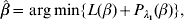 $$\hat{\beta } = \arg \min\! \lcub L( \beta ) + P_{\lambda _{{1}} } ( \beta ) \rcub , $$
with
 $$P_{\lambda _{{1}} } ( \beta ) = \mathop\sum\limits_{j = {1}}^{d} {\rho \left( {\left\Vert {\beta _{j} } \right\Vert_{\rm \Sigma _{j} }; \sqrt {d_{j} } \lambda _{{1}} , \gamma } \right)} .$$ $\rho ( t; \, \lambda , \gamma ) = \lambda \int_{{0}}^{\left\vert t \right\vert} {( 1 - ( x/ \lambda \gamma ) ) } + {\rm d}x$ is the MCP penalty (Zhang, Reference Zhang2010). $\left\Vert {\beta _{j} } \right\Vert_{\rm \Sigma _{j} } = \Vert {\rm \Sigma _{j}^{{1}/ {2}} \beta _{j} } \Vert_{{2}} $, $\vert \vert \cdot \vert \vert _{{2}} $ is the L 2 norm, $\rm \Sigma _{j} = n^{ - {1}} X_{j} {\prime } X_{j} $, and Xj is the n×dj submatrix of X that corresponds to βj. In (4), dj is the size of the coefficient group corresponding to gene j. When the M datasets have matched gene sets, dj≡M. We keep dj so that this formulation can easily accommodate partially matched gene sets. When gene j is not measured in dataset k, we take the convention $\beta _{j}^{k} \equiv 0$. λ1 is a tuning parameter, and γ is a regularization parameter.
In this analysis, genes are the functional units. The overall penalty is the sum over d individual penalties, with one for each gene. For gene selection, MCP penalization is adopted. For a specific gene, its effects in the M studies are represented by a ‘group’ of M regression coefficients. Under the homogeneity model, the M studies are expected to identify the same set of genes. Thus, within a group, no further selection is needed, and hence the L 2 norm is adopted. Note that here we adopt the  $\vert \vert \cdot \vert \vert _{\rm \Sigma _{j} } $ norm, which rescales the regression coefficient vector by covariance matrix Σj, so that computation is less ad hoc. This differs from the approach in Ma et al. (Reference Ma, Huang, Wei, Xie and Fang2011b) .
3. Heterogeneity model and penalized selection
(i) Heterogeneity model
When multiple datasets are generated in independent studies, heterogeneity inevitably exists (Knudsen, Reference Knudsen2006). The degree of heterogeneity depends on differences in study protocols, profiling techniques and many other factors. In cancer prognosis studies, the effort to unify the sets of identified markers across independent studies has not been very successful (Knudsen, Reference Knudsen2006; Cheang et al., Reference Cheang, van de Rijn and Nielsen2008). This can also be partly seen from Ma et al. (Reference Ma, Huang, Wei, Xie and Fang2011b) and our data analysis in Section 4. Such observations raise the question whether the homogeneity model is too restricted and motivates the heterogeneity model. Under the heterogeneity model, one gene can be associated with prognosis in some studies but not others. This model includes the homogeneity model as a special case and can be more flexible.
There are also scenarios under which the homogeneity model is conceptually not sensible, but the heterogeneity model is. The first is where different studies are on different types of cancers (Ma et al., Reference Ma, Huang and Moran2009). On the one hand, different cancers usually have different sets of markers. On the other hand, multiple pathways, such as apoptosis, cell cycle and signalling, are associated with prognosis of multiple cancers. The second scenario is the analysis of different subtypes of the same cancer. Different subtypes have different risks of occurrence and progression patterns, and it is not sensible to reinforce the same genomic basis. The third scenario is where subjects in different studies have different demographic measurements, clinical risk factors, environmental exposures and treatment regimens. For genes not intervened with those additional variables, their importance remains consistent across multiple studies. However, for other genes, they may be important in some studies but not others.
(ii) Penalized selection
Consider the penalized estimate
 $$\hat{\beta } = \arg \min\! \lcub L( \beta ) + P_{\lambda _{{1}} , \lambda _{{2}} } ( \beta ) \rcub , $$
where
 $$\eqalign {{P_{\lambda _{{1}} , \lambda _{{2}} } = \mathop\sum\limits_{j = {1}}^{d} {\rho \left( {\left\Vert {\beta _{j} } \right\Vert_{\rm \Sigma _{j} } ; \sqrt {d_{j} } \lambda _{{1}} , \gamma } \right)}} \cr \hskip30pt{+ \mathop\sum\limits_{j = {1}}^{d} {\mathop\sum\limits_{k = {1}}^{M} {\rho \left( {\left\vert {\beta _{j}^{k} } \right\vert; \, \lambda _{{2}} , \gamma } \right)}} .}}$$
Here, notations have similar definitions as in Section (ii). λ2 is another tuning parameter.
Under the heterogeneity model, marker selection needs to be achieved in two dimensions. The first is to determine whether a gene is associated with prognosis in any dataset at all. This step of selection is achieved using a GMCP penalty. For an important gene, the second dimension is to determine in which dataset(s) it is associated with prognosis. This step of selection is achieved using an MCP penalty. The sum of two penalties can achieve two-dimensional selection and fully recover the associations between multiple genes and prognosis in multiple studies.
In the single-dataset analysis with a continuous response and linear regression model, Friedman et al. (Reference Friedman, Hastie and Tibshirani2010) proposed a sparse group Lasso (SGLasso) penalty. The penalty in (5) has been partly motivated by that study. Owing to the analogy, we refer to penalty (5) as ‘sparse group MCP’ or SGMCP. Unlike in Friedman et al. (Reference Friedman, Hastie and Tibshirani2010), multiple heterogeneous datasets are analysed in this study, and a group corresponds to one gene in multiple datasets, as opposed to multiple variables. In addition, the MCP penalty is adopted to replace the Lasso penalty, as in single-dataset analysis, MCP has been shown to outperform Lasso (Zhang, Reference Zhang2010; Huang et al., Reference Huang, Breheney and Ma2012a, Reference Huang, Wei and Mab). In addition, censored survival data under the AFT model are analysed, which differ from the continuous response and linear model in Friedman et al. (Reference Friedman, Hastie and Tibshirani2010) . Note that MCP becomes Lasso when γ=∞. Thus, SGMCP includes SGLasso as a special case.
(iii) Computation
For dataset m(=1, …, M), we standardize the gene expressions to have marginal means zero and satisfy  $X_{j}^{m} {\prime } X_{j}^{m} = n$. Thus, $n^{ - {1}} X_{j}\! {\prime } X_{j} = {\rm I}_{d_{j} } $, where ${\rm I}_{d_{j} } $ is the dj×dj identity matrix. With slight abuse of notation, we denote $\vert \vert \beta _{j} \vert \vert \ {\rm for}\ \vert \vert \beta _{j} \vert \vert _{{\rm I}_{{d_{j} }} } $. For computation, we consider a GCD algorithm. It optimizes the objective function with respect to one gene at a time, and iteratively cycles through all genes. The overall cycling is repeated multiple times until convergence.
Consider the overall objective function
 $$\eqalign{\tilde L(\beta ,\lambda _1 ,\lambda _2 ,\gamma ) = & \displaystyle{1 \over {2n}}\left\| {Y - \sum\limits_{j = 1}^d {X_j \beta _j } } \right\|^2 \cr & + \sum\limits_{j = 1}^d {\rho \left( {\left\| {\beta _j } \right\|_{\Sigma _j } ;\sqrt {d_j } \lambda _1 ,\gamma } \right)} \cr & + \sum\limits_{j = 1}^d {\sum\limits_{k = 1}^M {\rho \left( {\left| {\beta _j^k } \right|;\lambda _2 ,\gamma } \right)} } .} $$
For j=1, …, d, given βk (k≠j) fixed at their current estimates  $\tilde{\beta }_{k}^{( s) } $, we seek to minimize $\tilde{L}( \beta , \lambda _{{1}} , \lambda _{{2}} , \gamma ) $ with respect to βj. Here, only the terms involving βj in $\tilde{L}<$><$>( \beta , \lambda _{{1}} , \lambda _{{2}} , \gamma ) $ matter. This is equivalent to minimizing
 $$\eqalign{R(\beta _j ) = & \displaystyle{1 \over {2n}}\left\| {r_{ - j} - X_j \beta _j } \right\|^2 + \rho \left( {\left\| {\beta _j } \right\|;\sqrt {d_j } \lambda _1 ,\lambda } \right) \cr & + \sum\limits_{k = 1}^M {\rho \left( {\left| {\beta _j^k } \right|;\lambda _2 ,\gamma } \right)} ,} $$
where 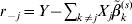 $r_{ - j} = Y - \sum\nolimits_{k \ne j} {X_{j} \tilde{\beta }_{k}^{( s) } } $. The first-order derivative of (7) is:
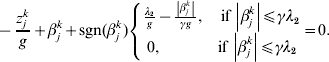
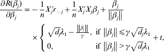 $$\eqalign{\displaystyle{{\partial R(\beta _j )} \over {\partial \beta _j }} = & - \displaystyle{1 \over n}X_j ^\prime r_{ - j} + \displaystyle{1 \over n}X_j ^\prime X_j \beta _j + \displaystyle{{\beta _j } \over {\left\| {\beta _j } \right\|}} \cr & \times \left\{ {\matrix{ {\sqrt {d_j } \lambda _1 - \displaystyle{{\left\| {\beta _j } \right\|} \over \gamma },\;{\rm if}\,\left\| {\beta _j } \right\| \le \gamma \sqrt {d_j } \lambda _1 } \cr {0,\;{\rm if}\,\left\| {\beta _j } \right\| \gt \gamma \sqrt {d_j } \lambda _1 } \cr } } \right. + t,} $$
where
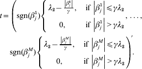 $$\eqalign{ t = \left( {{\rm sgn} ( \beta _{j}^{{1}} ) \left\{ {\matrix{ {\lambda _{{2}} - {{\left\vert {\beta _{j}^{{1}} } \right\vert} \over \gamma }, }\;{{\rm if}\, \left\vert {\beta _{j}^{{1}} } \right\vert\les \gamma \lambda _{{2}} } \cr {0, }\;{{\rm if}\,\left\vert {\beta _{j}^{{1}} } \right\vert \gt \gamma \lambda _{{2}} } \cr} , \ldots , } \right.} \right. \cr \left. {{\rm sgn} ( \beta _{j}^{M} ) \left\{ {\matrix{ {\lambda _{{2}} - {{\left\vert {\beta _{j}^{M} } \right\vert} \over \gamma }, }\;{{\rm if}\,\left\vert {\beta _{j}^{M} } \right\vert\les \gamma \lambda _{{2}} } \cr {0, }\;{{\rm if}\,\left\vert {\beta _{j}^{M} } \right\vert \gt \gamma \lambda _{{2}} } \cr} } \right.} \right){\prime} . \cr} $$
With normalization,  $n^{ - {1}} X_{j} ^{\prime } X_{j} = {\rm I}_{d_{j} } $. By setting expression (8) to be zero, we have:
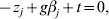 $$ - z_{j} + g\beta _{j} + t = 0, $$
where
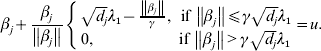
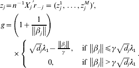 $$\eqalign{z_j = & n^{ - 1} X_j ^\prime r_{ - j} = (z_j^1 , \ldots ,z_j^M )' \cr g = & \left( {1 + \displaystyle{1 \over {\left\| {\beta _j } \right\|}}} \right) \cr & \times \left\{ {\matrix{ {\sqrt {d_j } \lambda _1 - \displaystyle{{\left\| {\beta _j } \right\|} \over \gamma },\quad {\rm if}\,\left\| {\beta _j } \right\| \le \gamma \sqrt {d_j } \lambda _1 } \cr {0,\quad {\rm if}\,\left\| {\beta _j } \right\| \gt \gamma \sqrt {d_j } \lambda _1 } \cr } } \right..} $$
We first take g fixed at the current estimate of βj. The kth element in (9) can be rewritten as:
 $$ - {{z_{j}^{k} } \over g} + \beta _{j}^{k} + {\rm sgn} ( \beta _{j}^{k} ) \left\{ {\matrix{ {{{\lambda _{{2}} } \over g} - {{\left\vert {\beta _{j}^{k} } \right\vert} \over {\gamma g}}, \quad {\rm if}\,\left\vert {\beta _{j}^{k} } \right\vert\les \gamma \lambda _{{2}} } \cr {0, \quad \hskip25pt{\rm if}\,\left\vert {\beta _{j}^{k} } \right\vert\les \gamma \lambda _{{2}} } \cr} } \right. = 0.$$
The solution to equation (10) is
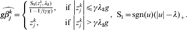 $$\widehat{g\beta _{j}^{k} } = \left\{ {\matrix{ {{{{\rm S}_{{1}} ( z_{j}^{k} , \lambda _{{2}} ) } \over {1 - 1/ ( \gamma g) }}, \quad {\rm if}\,\left\vert {z_{j}^{k} } \right\vert\les \gamma \lambda _{{2}} g} \cr {z_{j}^{k} , \quad \hskip21pt{\rm if}\,\left\vert {z_{j}^{k} } \right\vert \gt \gamma \lambda _{{2}} g} \cr} } \right.{\rm , \ S}_{{1}} = {\rm sgn} ( u) ( \vert u\vert - \lambda ) _{ + } .$$
 For k=1, …M, we set  $u_{k} = \widehat{g\beta _{j}^{k} }$ and $u = ( u_{{1}} , \ldots , u_{M} ) \prime$. Taking u back into its definition, we have
 $$\hskip-1pt\beta _{j} + {{\beta _{j} } \over {\left\Vert {\beta _{j} } \right\Vert}}\left\{ {\matrix{ {\sqrt {d_{j} } \lambda _{{1}} - {{\left\Vert {\beta _{j} } \right\Vert} \over \gamma }, \quad \hskip-6pt{\rm if}\,\left\Vert {\beta _{j} } \right\Vert\les \gamma \sqrt {d_{j} } \lambda _{{1}} } \cr {0, \quad \hskip42pt {\rm if}\,\left\Vert {\beta _{j} } \right\Vert \gt \gamma \sqrt {d_{j} } \lambda _{{1}} } \cr} } \right. = u.$$
Solving equation (11) leads to
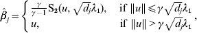 $$\hat{\beta }_{j} = \left\{ {\matrix{ {{\gamma \over {\gamma - 1}}{\rm S}_{{2}} ( u, \sqrt {d_{j} } \lambda _{{1}} ) , \quad {\rm if}\,\left\Vert u \right\Vert\les \gamma \sqrt {d_{j} } \lambda _{{1}} } \cr {u, \quad \hskip62pt{\rm if}\,\left\Vert u \right\Vert \gt \gamma \sqrt {d_{j} } \lambda _{{1}} } \cr} } \right., $$
where 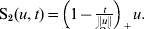 ${\rm S}_{{2}} ( u, t) = \left( {1 - {t \over {\left\Vert u \right\Vert}}} \right)_{ + } u.$
Solving equation (9) amounts to iteratively calculating equation (10)–(12) until convergence. Overall, with fixed tuning parameters,
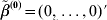
1. Initialize s=0, the estimate $\tilde{\beta }^{( {0}) } = ( 0, \ldots , 0) \prime$, and the vector of residuals $r = Y - \sum\nolimits_{j = {1}}^{d} {X_{j} \tilde{\beta }_{j}^{( {0}) } } $;
2. For j=1, …, d,
(a) Update
$\tilde{\beta }_{j}^{( s + {1}) } $. This is achieved by solving equation (9)–(12) iteratively until convergence. In our numerical study, convergence is achieved for all datasets within ten iterations;(b) Update
$r \leftarrow r - X_{j} ( \tilde{\beta }_{j}^{( s + {1}) } - \tilde{\beta }_{j}^{( s) } ) $;
3. Update s←s+1;
4. Repeat Steps 2–3 until convergence.


This algorithm starts with a null model. In each iteration, it cycles through all d genes. For each gene, it only involves simple calculations, and the update can be accomplished easily. We use the L 2 norm of the difference between two consecutive estimates smaller than 10−5 as the convergence criterion. Convergence is achieved with all our simulated and real data.
(iv) Tuning parameter selection
With the MCP penalty, there is one tuning parameter λ and one regularization parameter γ. Generally speaking, smaller values of γ are better at retaining the unbiasedness of the MCP penalty for large coefficients, but they also have the risk of creating objective functions with a non-convexity problem that are difficult to optimize and yield solutions that are discontinuous with respect to λ. It is therefore advisable to choose a γ value that is big enough to avoid this problem but not too big (Zhang, Reference Zhang2010; Breheny & Huang, Reference Breheny and Huang2011). Such results can be extended to the SGMCP.
In principle, it is possible to have different γ values for the two penalties. In practice, adopting the same γ value may reduce computational cost without affecting performance of the estimate much. In numerical study, we have experimented with a few values for γ, particularly including 1·8, 3, 6 and 10 and ∞, as suggested in Zhang (Reference Zhang2010) and Breheny & Huang (Reference Breheny and Huang2011) . λ1 and λ2 control shrinkage at the group and individual-coefficient levels, respectively. Let λ2max be the largest λ2 for which all regression coefficients are shrunk to zero. Let λ1max(λ2) be the largest λ1 under a fixed λ2 for which all regression coefficients are shrunk to zero. It can be shown that  $\lambda _{{2}\max } = <$> <$>n^{ - {1}} \max _{j = {1}, \ldots , d, k = {1}, \ldots , M} \vert {X_{j}^{k} Y^{k} } \vert$, where $X_{j}^{k} $ is the component of Xj that corresponds to the kth dataset. $\lambda _{{1}\max } ( \lambda _{{2}} ) = \max _{j = {1}, \ldots , d} \left\Vert {{\rm S}_{{1}} ( n^{ - {1}} X_{j} {\prime } Y, \lambda _{{2}} ) } \right\Vert/ \sqrt {d_{j} } $. This result puts constraints on the range of tuning parameters.
In this study, we search for γ, λ1 and λ2 values jointly using V-fold cross-validation (V=5 in numerical study). This is computationally feasible as the GCD algorithm has low computational cost. It is expected that λ1, λ2 cannot go down to very small values that correspond to regions not locally convex. The cross-validation criteria in such non-locally convex regions may not be monotonous. To avoid such regions, we select λ1 and λ2 where the cross-validation criterion first goes up.
4. Numerical study
(i) Simulation
We simulate three datasets, each with 100 subjects. For each subject, we simulate the expressions of 1000 genes. The gene expressions are jointly normally distributed, with marginal means equal to zero and variances equal to one. We consider two correlation structures. The first is the auto-regressive (AR) correlation, where expressions of genes j and k have correlation coefficient ρ|j−k|. We consider two scenarios with ρ=0·2 and 0·7, corresponding to weak and strong correlations, respectively. The second is the banded correlation. Here, two scenarios are considered. Under the first scenario, genes j and k have correlation coefficient 0·33 if |j−k|=1 and 0 otherwise; under the second scenario, genes j and k have correlation coefficient 0·6 if |j−k|=1, 0·33 if |j−k|=2, and 0 otherwise. We consider the heterogeneity model, under which each dataset has 10 prognosis-associated genes. The three datasets share five common important genes, and the rest prognosis-associated genes are dataset-specific. As a special case of the heterogeneity model, we also consider the homogeneity model, under which all three datasets share the same 10 prognosis-associated genes. Under both models, across the three datasets, there are a total of 30 true positives. For the mth dataset, we generate the logarithm of event time from the AFT model:  $T^{m} = \beta _{{0}}^{m} + X^{m\prime} \beta ^{m} + \varepsilon ^{m} $, where $\beta _{{0}}^{m} = 0{\cdot}5$ and ∊m∼N(0, 0·25). The non-zero regression coefficients for β1, β2 and β3 are (0·4, 0·4, 0·6, −0·5, 0·3, 0·3, 0·6, 0·5, 0·5, 0·2), (0·5, 0·2, 0·3, −0·5, 0·4, 0·4, 0·3, 0·2, 0·6, 0·5) and (0·6, 0·3, 0·7, −0·4, 0·5, 0·3, 0·5, 0·7, 0·4, 0·3), respectively. The logarithm of censoring time is generated as uniformly distributed and independent of the event time. We adjust the censoring distributions so that the overall censoring rate is about 30% under all simulation scenarios. In the Appendix, we also present simulation results under ∊1∼0·2t(60), ∊2∼0·6t(30), ∊3∼t(20), that is, the three datasets have different error distributions with different variances.
For a simulated dataset, we analyse using SGMCP as well as the following alternatives: (i) MCP and Lasso (which is MCP with γ=∞). Here, we analyse the three datasets separately and then combine analysis results across datasets. This is a meta-analysis approach. (ii) GMCP and GLasso (which is GMCP with γ=∞). These two approaches reinforce that the same set of genes are identified across datasets, are sensible under the homogeneity model, but can be too restricted under the heterogeneity model; and (iii) SGLasso (which is SGMCP with γ=∞). With the above approaches, we consider three different γ values for the MCP and GMCP penalties. For all approaches, tuning parameters are chosen using 5-fold cross-validation.
Summary statistics, including the number of true positives, number of false positives, and their standard deviations based on 100 replicates, are shown in Table 1 (homogeneity model, homogeneous errors) and 2 (heterogeneity model, homogeneous errors) and 5 (Appendix, homogeneity model, heterogeneous errors) and 6 (Appendix, heterogeneity model, heterogeneous errors), respectively. We observe that SGMCP has the best performance under all simulated scenarios. It can significantly outperform GMCP under the homogeneity model. SGMCP is able to identify most or all of the true positives. Under some simulated scenarios, there are a number of false positives. This is partly caused by correlations among genes. The false positive rate increases as genes become ‘more correlated’. When γ increases, then the number of false positives increases. This is as expected, as in single-dataset analysis, it has been suggested that Lasso-type penalization (γ=∞) tends to overselect (Huang et al., Reference Huang, Breheney and Ma2012a). GMCP and MCP may identify a satisfactory number of true positives, however, at the price of a much larger number of false positives (Table 2).
Table 1. Simulation under the homogeneity model. In each cell, the first/second row is the mean number (sd) of true/false positives. When γ=∞, MCP simplifies to Lasso

Table 2. Simulation under the heterogeneity model. In each cell, the first/second row is the mean number (sd) of true/false positives. When γ=∞, MCP simplifies to Lasso

(ii) Analysis of breast cancer studies
Worldwide, breast cancer is the commonest cancer death among women. In 2008, breast cancer caused 458 503 deaths worldwide (13·7% of cancer deaths in women). Multiple high-throughput profiling studies have been conducted, searching for genomic markers associated with breast cancer prognosis. We collect data from three independent breast cancer prognosis studies, which were originally reported in Huang et al. (Reference Huang, Cheng, Dressman, Pittman, Tsou, Horng, Bild, Iversen, Liao, Chen, West, Nevins and Huang2003), Sotiriou et al. (Reference Sotiriou, Neo, McShane, Korn, Long, Jazaeri, Martiat, Fox, Harris and Liu2003) and van't Veer et al. (Reference Van 't Veer, Dai, van de Vijver, He, Hart, Mao, Peterse, van der Kooy, Marton, Witteveen, Schreiber, Kerkhoven, Roberts, Linsley, Bernards and Friend2002), respectively, and referred to as D1, D2 and D3 hereafter. In D1, Affymetrix chips were used to profile the expressions of 12 625 genes. There were a total of 71 subjects, among whom 35 died during follow-up. The median follow-up was 39 months. In D2, cDNA chips were used to profile the expressions of 7650 genes. There were a total of 98 subjects, among whom 45 died during follow-up. The median follow-up was 67·9 months. In D3, oligonucleotide arrays were used to profile 24 481 genes. There were a total of 78 patients, among whom 34 died during follow-up. The median follow-up was 64·2 months. We process each dataset separately as follows. With Affymetrix data, a floor and a ceiling are added, and then measurements are log 2 transformed. With both Affymetrix and cDNA data, we fill in missing expressions with means across samples. We then standardize each gene expression to have zero mean and unit variance.
In previous studies such as Ma et al. (Reference Ma, Huang, Wei, Xie and Fang2011b), the homogeneity model is assumed. As the three datasets were generated in three independent studies, heterogeneity is expected to exist across datasets. This can be partly seen from the summary survival data, the profiling protocols, as well as results from analysis of each individual dataset using MCP (Table 7). We analyse the three datasets using the proposed approach as well as MCP, GMCP and SGLasso. The identified genes and corresponding estimates are shown in Tables 3 and 7–9 in the Appendix. Note that with all approaches, the small magnitudes of regression coefficients are caused by ‘clustered’ log survival times. SGMCP identifies seven, eight and five genes for D1–D3, respectively. Estimates in Table 3 suggest that different datasets may have different prognosis-associated genes. This partly explains why it fails to unify the identified markers across different breast cancer prognosis studies (Cheang et al., Reference Cheang, van de Rijn and Nielsen2008) . As described in Section 1, multiple factors may contribute to this heterogeneity. Without having access to all the experimental details, we are not able to determine the exact cause of heterogeneity. Although there are overlaps, different approaches identify significantly different sets of genes. This observation is not surprising given the simulation results. We mine the published literature and find that genes identified by SGMCP may have important biological implications. More details are provided in the Appendix. Of note, as there is no objective way to determine which set of genes are ‘biologically more meaningful’, we do not discuss the biological implications of genes identified by the alternative methods.
Table 3. Analysis of breast cancer data using SGMCP: identified genes and their estimates
To provide a more comprehensive description of the three datasets and various approaches, we also conduct evaluation of prediction performance. Although, in principle, marker identification and prediction are two distinct objectives, evaluation of prediction performance can be informative for marker identification. In particular, if prediction is more accurate, then the identified markers are expected to be more meaningful. For prediction evaluation, we adopt a random sampling approach as in Ma et al. (Reference Ma, Huang and Moran2009) . More specifically, we generate training sets and corresponding testing sets by random splitting data with sizes 3 : 1. Estimates are generated using the training sets only. We then make prediction for subjects in the testing sets. We dichotomize the predicted linear risk scores  $X \prime \hat{\beta }$ at the median, create two risk groups, and compute the logrank statistics, which measure the difference in survival between the two groups. To avoid extreme splits, this procedure is repeated 100 times. The average logrank statistics are calculated as 7·30 (SGMCP), 3·43 (MCP), 2·77 (GMCP) and 3·33 (SGLasso). SGMCP is the only approach that can separate subjects into groups with significantly different survival risks (P-value=0·007). Such a result suggests that allowing for heterogeneity in markers across datasets can lead to better prediction performance.
(iii) Analysis of lung cancer studies
Lung cancer is the leading cause of death from cancer for both men and women in USA and in most other parts of the world. Non-small-cell lung cancer (NSCLC) is the most common cause of lung cancer death, accounting for up to 85% of such deaths (Tsuboi et al., Reference Tsuboi, Ohira, Saji, Hiyajima, Kajiwara, Uchida, Usuda and Kato2007). Gene-profiling studies have been extensively conducted on lung cancer, searching for markers associated with prognosis. Data were collected from three independent experiments (Shedden et al., Reference Shedden, Taylor, Enkemann, Tsao, Yeatman, Gerald, Eschrich, Jurisica, Giordano, Misek, Chang, Zhu, Strumpf, Hanash, Shepherd, Ding, Seymour, Naoki, Pennell, Weir, Verhaak, Ladd-Acosta, Golub, Gruidl, Sharma, Szoke, Zakowski, Rusch, Kris, Viale, Motoi, Travis, Conley, Seshan, Meyerson, Kuick, Dobbin, Lively, Jacobson and Beer2008; Jeong et al., Reference Jeong, Xie, Xiao, Behrens, Girard, Wistuba, Minna and Mangelsdorf2010; Xie et al., Reference Xie, Xiao, Coombes, Behrens, Solis, Raso, Girard, Erickson, Roth, Heymach, Moran, Danenberg, Minna and Wistuba2011). The UM (University of Michigan Cancer Center) study had a total of 175 patients, among whom 102 died during follow-up. The median follow-up was 53 months. The HLM (Moffitt Cancer Center) study had a total of 79 subjects, among whom 60 died during follow-up. The median follow-up was 39 months. The CAN/DF (Dana-Farber Cancer Institute) study had a total of 82 patients, among whom 35 died during follow-up. The median follow-up was 51 months. 22 283 genes were profiled in all three studies.
In studies such as Xie et al. (Reference Xie, Xiao, Coombes, Behrens, Solis, Raso, Girard, Erickson, Roth, Heymach, Moran, Danenberg, Minna and Wistuba2011), the three datasets were combined and analysed. Such a strategy corresponds to the homogeneity model. Here, we analyse using SGMCP (Table 4), MCP (Table 10), GMCP (Table 11) and SGLasso (Table 12). The observed estimation patterns are similar to those for the breast cancer data. The SGMCP estimates again suggest that different datasets may have different prognosis-associated genes. In the Appendix, we show that the SGMCP identified genes may have important biological implications. We also evaluate prediction performance using the resampling approach described in the last subsection. The average logrank statistics are calculated as 10·93 (SGMCP), 2·83 (MCP), 1·73 (GMCP) and 3·07 (SGLasso), respectively. The observation is again similar to that for the breast cancer data.
Table 4. Analysis of lung cancer data using SGMCP: identified genes and their estimates
5. Discussion
In cancer genomic research, multi-dataset analysis provides an effective way to overcome certain drawbacks of single-dataset analysis. In most published studies, it has been reinforced that multiple datasets share the same set of prognosis-associated genes, that is, the homogeneity model. In this study, for multiple cancer prognosis datasets, we consider the heterogeneity model, which includes the homogeneity model as a special case and is less restricted. This model may provide a way to accommodate the failure to unify cancer prognosis markers across independent studies (Knudsen, Reference Knudsen2006; Cheang, Reference Cheang, van de Rijn and Nielsen2008). Under the heterogeneity model, we use sparse group penalization for marker identification. This penalization approach is intuitively reasonable and computationally feasible. Simulation study shows that it has satisfactory performance. It is interesting to note that SGMCP outperforms GMCP even under the homogeneity model. Thus, in practical data analysis, the heterogeneity model and SGMCP can be a ‘safer’ choice. With the breast cancer and lung cancer prognosis datasets, existing analyses assume the same set of markers across datasets. Our analysis suggests that it may be more reasonable to allow for different sets of markers.
Under the heterogeneity model, marker identification needs to be conducted in two dimensions. Beyond sparse group penalization, composite penalization and multi-step approaches may also be able to achieve such identification. In this paper, we focus on sparse group penalization. Comprehensive investigation and comparison of different approaches are beyond the scope of this paper. The proposed approach is based on the MCP penalty, which has been shown to have satisfactory performance in single-dataset analysis. We suspect that it is possible to develop similar approaches based on, for example, bridge and SCAD penalties. As in single-dataset analysis there is no evidence that such penalties are superior to MCP, such a development is not pursued. In our numerical study, we observe superior performance of the proposed approach. A limitation of this study is lack of theoretical support. Pursuit of theoretical properties is postponed to future studies.
We thank the editor, associate editor and two reviewers for careful review and insightful comments. Part of the study was conducted when the first author was at Yale University. The authors have been supported by awards CA142774, CA165923 and CA152301 from NIH, DMS0904181 and DMS1208225 from NSF, 2012LD001 from the National Bureau of Statistics of China, and the VA Cooperative Studies Programme of the Department of Veterans Affairs, Office of Research and Development.
The appendix for this paper is available online at the journal's website (http://journals.cambridge.org/grh).


