1. Introduction
The physics of the flow of water in glaciers contains a rich variety of interesting problems. The mechanics and the thermodynamics of water flow through the intercrystalline vein system (Reference Nye and FrankNye and Frank, 1973), through a thin sheet at the bed of the glacier, and through a tunnel at the bottom of the glacier or elsewhere within the glacier, have much in common. At the same time these different flows can present apparent contradictions and delicate questions. For example, water flow through a subglacial tunnel can generate enough heat by friction to enlarge the tunnel in a catastrophic way; but water flow through the vein system, if it occurs, evidently does not normally do this. Why should this be so? During a catastrophic outburst from an ice-dammed lake does the water necessarily flow beneath the glacier within discrete channels or can it flood out into a basal sheet? When a catastrophic outburst is in full spate how can it end prematurely, before it has exhausted the supply of water? These are some of the questions we wish to discuss.
General mathematical treatments of the flow of water in glaciers have been given, in particular, byReference RöthlisbergerRöthlisberger (1972), Reference ShreveShreve (1972), and Wcertman (1972). This paper has a different emphasis because, although much of the treatment tries to be general, we shall continually refer to a special and unusual phenomenon: the periodic draining of Grimsvötn, the subglacial ice-dammed lake in the centre of the ice cap Vatnajökull in Iceland; see Reference BjörnssonBjörnsson ([1975]),Reference TómassonTómasson ([1975]) and the recent book by Reference ThorarinssonThorarinsson (1974). The draining of the lake, which used to happen about every 10 years and now happens about every 5 years, is accompanied by an enormous outburst of water (a jökulhlaup) from beneath the ice edge to the sea, the outburst place being 50 km from the lake itself (Fig. 1). For example, the outburst of 1934 (Reference ThorarinssonThorarinsson, 1953, 1957), which was a normal one for that period, carried at its climax 4 to 5 x 10⁴ m3 s-1 of muddy water (about a quarter of the flow of the River Amazon, and more than that of the River Congo) bringing with it “icebergs as big as three-storeyed houses”. Almost the whole of the sandur, or outwash plain, some 1 000 km2 in area, was flooded. But by the next morning the flow of the main outlet river, Skeiôarâ, had returned to normal. Any road along the south coast of Iceland had to cross the outwash plain and so it is not surprising that for many years none was built. Nevertheless, the construction of a road and bridges has been undertaken since the last outburst in 1972 (when the maximum How was 8 x 10³ m3 s-I) in spite of the confident expectation of the next one in about 1977 or 1978. It is therefore practically important as well as scientifically interesting to understand the Grimsvötn phenomenon fully.

Fig. 1. Vatnajökull ice cap, showing Grímsvötn, the subglacial ice-dammed lake, and the presumed route (broken line) of the ice tunnel system, 50 km long, under the glacier Skeiðarárjökull. The road recently constructed across the outwash plain, Skeidaðarársandur, in the path of the outbursts is shown by the broken line between the glacier and the coast. Contour heights in metres. From Reference BjörnssonBjörmsson ([1975]).
There are many other examples of catastrophic outbursts from ice-dammed lakes and various different types are recognized; we may mention especially the accounts by Reference ThorarinssonThorarinsson (1939) and Reference Licst ølLiestøl (1956) and the useful short summary in the book by Reference Embleton and KingEmbleton and King (1968); for other references see the paper by Reference WhalleyWhalley (1971). We do not attempt a full treatment of the whole subject here, rather we try to analyse in some detail various aspects and puzzles of glacier hydraulics which are thrown into prominence by the j ökulhlaup phenomenon.
Section 2 outlines our interpretation of the Grimsvötn phenomenon and Section 3 deals with the physics of the lake seal in more detail. Section 4 sets up the general differential equations for non-steady flow in tunnels, and these are applied specifically to the 1972 Grimsvötn flood in Section 5 to explain the observed discharge hydrograph and the abrupt ending of the flood. Section 6 discusses the essential difference which can make a waterway behave stably, as in drainage through a vein, or unstably, as in a flood in a subglacial tunnel. Finally, we consider why Grimsvötn does not drain out through the vein system (Section 7) and under what conditions glacial lakes in general will drain in this way (Section 8).
2. An Outline Interpretation of the Grímsvötn Phenomenon
The essentials of the Grimsvötn phenomenon as interpreted by Helgi Björnsson and the author, building on the work of many previous writers, can be modelled as follows. In his separate paper, which is complementary to the present one, Reference BjörnssonBjörnsson ([1975]) has compiled the necessary detailed topographical information and has made numerical calculations based on the most accurate surveys.
A geothermal area at the base of the ice cap, shown schematically in Figure 2, causes melting and thereby creates a depression in the upper surface. Thus the run-off from the top surface generated by the ordinary processes of ablation no longer flows entirely towards the edges of the ice cap, as it would normally do, but part of it flows into the depression. Water accumulates in a lake (shown shaded), generated both by the surface run-off" and by geothermal melting. In Grimsvötn roughly 25% comes from run-off and 75% from geothermal melting. Grimsvötn is almost completely covered by a floating plug of ice some 220 m thick, which is essentially an ice shelf.
It is commonly supposed that the floods from ice-dammed lakes start by the lifting of the ice dam by flotation (Reference StrømStrom, 1938; Reference ThorarinssonThorarinsson, 1939), and Reference ThorarinssonThorarinsson (1953, 1957) suggested that this was the case with Grimsvötn—although, later on, incomplete topographic information led him to doubt whether flotation was possible in this instance (Reference ThorarinssonThorarinsson, 1965). Let us examine the flotation hypothesis. Suppose the water level in the lake at a given time while it is filling is L (Fig. 2). We can construct the broken curves B, obtained by reflecting the ice-cap surface in L and magnifying its vertical scale by a factor ρi(ρw—ρi), where ρi and ρw are the densities of ice and water; the factor is about 10. To see the meaning of curves B, keep the top surface of the ice cap fixed and imagine the whole ice cap immersed in an ocean whose surface level is L. Curves B represent the bottom surface the ice mass would then need to have if it simply floated, like an iceberg, in isostatic balance in the water (the “iceberg” would need to have negative thickness outside points M and N).

Fig. 2. Schematic section through the ice cup. The lake (shaded) is seated along DE and FG.
We see that along DE and FG the ice is “grounded” if water existed outside D and G in hydrostatic communication with the lake its pressure would be more than enough to lift the ice. Thus the absence of any such hydrostatic connexion is vital to preserving the lake. In plan view the grounding takes place over an annulus, and it is this that seals the lake.
Figure 3 shows the critical part of the seal FG in magnified form and to scale, but with vertical exaggeration. The lake level now rises from L and so curve B also rises (II times faster).

Fig. 3. The critical part of the seat, to scale with vertical exaggeration 20, Full lines are the glacier bed and surface. Topography fromReference BjörnssonBjörnsson ([1975]) .
The critical condition is reached when B reaches B' SO that it just touches the bed curve at K; at this point the seal breaks. In three dimensions one has to visualize the inverted and magnified top surface moving upwards and eventually touching the bed surface; the point of contact of the two surfaces is the critical point κ, where the width of the sealing annulus is reduced to zero. (To visualize the topology consider the intersection of a horizontal plane with a curved surface near a saddle point, and then tilt both surfaces together.)
In fact the flood occurs with the lake level still some 20 m below the level that this model would predict. According toReference BjörnssonBjörnsson ([1975]) this discrepancy is unlikely to be due to errors in the survey, and in the next section we suggest an explanation based on the fact that the ice exerts slightly less pressure on the bed than would be given by the weight of a free column. (We may remark here that Reference GlenGlen's mechanism (1954) would require a lake level 20 m above rather than 20 m below the prediction of the simple floating model.)
As soon as water penetrates the seal one possibility would be simply a slow subglacial overflow from the lake. There would be no jökulhlaup; a steady outflow through the seal would just balance the inflow to the lake. But we shall see (Section 6) that such a condition, although a steady state, is inherently unstable. This is the essential instability that is responsible for the jökulhlaup.
Accordingly, a subglacial channel system is opened up unstably by the flowing water, which moves towards the edge of the ice cap, the preferred route (Fig. 1), 50 km long, running beneath one of the outlet glaciers, Skeiöararjökull. Does the water flow under the glacier in one or more confined channels or tunnels, or does it possibly flow in the form of a continuous sheet at the glacier bed? The water is seen to emerge from beneath the ice front of Skeiöararjökull in two major and several minor channels, and collapsed “cauldrons” visible in satellite photographs (Reference BjörnssonBjörnsson, [1975]) suggest that for 10-15 km below the seal the water is in a channel; but from an observational point of view the water could be equally well in a fairly wide sheet or in a tunnel for the greater part of its course. Of course, the fact that the glacier itself does not surge forward during the flood sets some limits to the type and extent of the water sheet that one could contemplate. Detailed calculation shows that the hypothesis of one or several tunnels gives excellent agreement with the observations, and therefore we favour this model.
In a tunnel the water pressure p is less than the pressure p i that would be given simply by the weight of the overlying glacier and so it tends to close by plastic deformation of the ice, but at the same time the frictional heat from the turbulent flowing water tends to enlarge the tunnel by melting (Reference RöthlisbergerRöthlisberger, 1972). The melting rate dominates and the flood grows catastrophically in the way envisaged by Reference Licst ølLiestol (1956).
Now we have to ask what stops it. It might be expected to continue at least until the level L of the lake fell to the rim J (Fig. 3). In fact the flood stops after the water level in the lake has fallen only 100 m and is still 230 m above J (Reference BjörnssonBjörnsson, [1975]). The seal reforms—in spite of frictional melting by the torrential flow of water—and the suggested explanation, which differs slightly from Reference BjörnssonBjörnsson's ([1975]), is this. As the lake level falls, so does the pressure in the tunnel. Although this causes faster plastic closing, it is overwhelmed at first by the melting rate. Later on, however, when the flood is very great, the lake level is falling very rapidly and so is the pressure in the tunnel. We show later that, if τ measures the time remaining before asymptotic catastrophe, the pressure difference tending to close the tunnel increases at least as fast as I + (τo/τ)3, τo being a constant, and the associated strain-rate at least as fast as {I +(τ0/τ)3)3, which is an extremely strong time dependence, approaching T-9 Thus, quite suddenly, the plastic closure rate catches up with the melting rate and the flood rapidly abates. The seal is reformed.
This completes our qualitative outline of how the jökulhlaup starts and how it ends. We now examine the various assertions in more detail.
3. Hydrostatic Theory. Filling of the Lake
The hydrostatics of the seal can be presented in several different ways. It is instructive to look at it now from a slightly different point of view.
Let zb be the height of the glacier bottom (Fig. 4) and zs be the height of the glacier surface, taking as datum the level of the eventual water exit at the snout of the glacier. The thickness of the glacier is given by h = z s-z b Let us consider the situation between jökulhlaups, while the lake is filling. At the glacier bed we may suppose there is a thin film of water at a pressure p, say. If s is a coordinate measured down-glacier parallel to the bed, the effective negative pressure gradient driving the water towards the snout is
say, where the potential φ is given by
If we take p to be the ice overburden pressure pigh,

Fig. 4. Schematic section to illustrate the hydrostatics of the seal.
Figure 4 shows schematically a graph of φ(s) obtained essentially by drawing the bottom profile z b of the glacier and adding to it 0.91 of the glacier thickness (it is similar to Röthlis-berger's “water-equivalent line”). Point F on the bed is the uppermost point of the water film, where the glacier goes afloat. Here the pressure in the water sheet must equal the hydrostatic pressure from the lake. Thus the lake surface, at height z0, passes through v, the point on the curve of φ vertically above F. The lake is now sealed (with φ > ρwgz 0) between F and G. If we assumed that as the lake level rose the glacier ice did not move vertically at all, the curves to the right of F would all remain fixed, the intersection point v would move to the right and the seal at κ would be broken when v reached M, the maximum of the φ curve vertically above κ. This would correspond to the hydrostatic argument of the last section. But it needs correction because the ice between F and κ, if not melted sufficiently by the advancing lake water, will be subject to a buoyancy force which will bend it upwards and thus reduce the pressure at the bottom of the still-grounded ice. The reduction of pressure occurs because the submerged ice does not immediately attain isostatic balance and so acts on the grounded ice as a buoyant inverted cantilever. The result is that p in Equation (2) will be a little less than pigh, φ will be correspondingly less and M will be lower.
The magnitude of this effect may be crudely estimated by assuming the ice to be perfectly plastic with yield stress k. The maximum vertical shear traction the cantilever can exert on the grounded ice is k. Suppose the vertical shear stress thus set up drops to zero over a length L’ of the grounded ice. Then, considering unit width, the force exerted on the bed from the weight of the ice in the length L', which is pighL’, is diminished by kh, and thus the pressure on the bed will be pigh-k(h/L’). If the transition length L = ½h, which is quite reasonable, this provides a reduction in pressure of 2k, which with a yield stress of I bar is just equivalent to the required 20 m of water. (I bar is an appropriate value for k because the lake takes several years to fill and so the rate of deformation is correspondingly small.) So the effect of the buoyant cantilever in prising open the seal gives a good reason why the flood starts when the lake level is still 20 m below the level the simple lifting model would predict. Note that by the construction κ lies, in plan view, between the summit N of the ice surface and the summit J of the bed, as we saw in Section 2 (these points are of course not necessarily true summits but only maxima in the profile drawn). The condition at the critical point is evidently dφ/ds = o. Ignoring the correction and using Equation (3), with h = zs—zb , this gives
or, in terms of the slopes of the upper surface α and the lower surface β, roughly
α = —1/10β.
That is to say, above κ the backward slope of the upper surface is one-tenth of the forward slope of the bed, a relationship that is already evident by inspection of Figure 3.
Before the seal is broken, the thin water sheet at the bed of the glacier has a divide at κ. Up-stream from κ it flows uphill to the lake; down-stream from κ it flows towards the snout. We return to this point when discussing the role of the intergranular veins in Section 7.
4. Differential Equations for Time-Dependent Water Flow in Tunnels in Glaciers
In this section we derive the general differential equations which govern- the non-steady flow of water in a conduit within a glacier, the conduit being simultaneously melted by the heat of friction and contracted by plastic deformation in the way discussed by Reference RöthlisbergerRöthlisberger (1972). The conduit, which is assumed to be completely filled with water, can be thought of as a normal internal glacier water-course or as a large tunnel associated with a jökulhlaup. The change of specific volume on melting, the work associated with the change of diameter by melting and plastic deformation, the dependence of melting point on pressure, and the matter of temperature gradients across and along the tunnel all make it necessary to be careful with the thermodynamics. Readers who prefer to skip the details may like to go straight to the final equations (16)-(20). Related treatments have been given byReference RöthlisbergerRöthlisberger (1972), who was primarily concerned with steady How, Reference ShreveShreve (1972),Reference MathewsMathews (1973), and Reference WeertmanWeertman (1972).
Consider an inclined water-filled conduit (Fig. 5) of cross-sectional area S, which is a function of position s and time t. ∂S/∂t is made up of two parts, one due to melting and one due to plastic, deformation which we denote (∂S/∂t) Thus
where m(s, t) is the mass melted per unit length per unit time, and v i = ρi -1 is the specific volume of ice. If Q(s, t) denotes the volume of water flowing through a cross-section per unit time, the discharge, we may write the continuity equation for the water flow as
where vw = ρw -1 is the specific volume of water. Eliminating ∂S/∂t between Equations (4) and (5) gives
where Δν = vw — vi is the change in specific volume on melting, For the rate of plastic deformation we shall write
Here pi is the ice overburden pressure, p is the pressure in the water and Ko is a constant depending on the shape of the cross-section. If the cross-section were circular and we used the Glen flow law for ice, this equation would be exact and n would be about 3 (Reference NyeNye, 1953). It is plausible to assume that even with a non-circular section the rate will be proportional to a high power of the pressure difference.

Fig. 5. The thermodynamic system.
To apply the first law of thermodynamics we consider the system consisting of a short length l of the conduit, the end boundaries to the system moving with the water; thus l is a function of s and t. As the conduit contracts by plastic deformation, work is done by the external pressure. In time δt some ice will be melted and it is therefore convenient to place the cylindrical (or, more strictly, conical) boundary of the system so that it just includes the ice which is about to be melted. Thus the cylindrical boundary is fixed relative to the solid, but it moves because of plastic deformation. The mass within the system is fixed. The rate of work done on the system at the cylindrical boundary is then
The rate of work by the water pressure on the up-stream boundary is pQ and the total rate of work by both up-stream and down-stream boundaries together is
The rate of work done by gravity is Qρwgsl, where gs is the j-component of gravity. Thus the total rate of work done on the system per unit length is
We wish to know the rate of increase in internal energy of the system. The flow being turbulent, nearly all the water will be well mixed and at a temperature θw (s, t), say, but at the ice wall there will be a thin boundary layer across which the temperature falls θi (s, t) the melting point of ice appropriate to the water pressure. During time δt the water within the system consists of two parts: the water already present at time t and the new water being formed by melting. The total change of internal energy δU is thus the sum of two terms:
Here σ is the specific heat capacity of water, d/dt is the derivative following the element, Δu is the difference of internal energy per unit mass between water and ice at the melting point, and the water is taken to be incompressible. The first term is the internal energy needed to raise the temperature of the already existing water; the second term is the internal energy needed to melt the new water and raise it to temperature θw (the boundary layer is assumed to remain the same, gaining water on one side and losing it on the other). Note that in the first term the volume Sl is left outside the differentiation because this part of the water remains fixed in volume. We are neglecting any contribution from kinetic energy.
If we neglect conduction of heat across the ends of our moving system, the heat input to the system is zero; so the first law of thermodynamics enables us to equate the rate of work given by Equation (8) with the rate of increase of internal energy given by Equation (9). In doing so we make use of the general thermodynamical relation
L being the latent heat per unit mass. Hence
and substitution for (∂S/t)pi from Equation (6) reduces this to
Equation (11) has the physical interpretation that if the system is taken to be only the entering water volume Q without the addition made by melting, Qρwgs is the work done by gravity, —Q ∂p/∂s is the work done by the water pressure at the ends, ρw σS (dθ w/dt) is the heat output used to raise the temperature of the water and the right-hand side is the heat output used in melting. However, to derive Equation (11) on these lines raises questions about the work done against the lateral pressure and the shear forces—questions which are avoided by the slightly longer, but we hope clearer, treatment we have given.
There is a further relation between the pressure gradient, the flow Q and the cross-section S of the conduit. Following Reference RöthlisbergerRöthlisberger (1972) and Reference MathewsMathews (1973) we use the empirical Gauckler-Manning formula (Reference WilliamsWilliams, 1970) for the mean velocity ü = Q/S for turbulent flow, thus
where R is the hydraulic radius (cross-section divided by perimeter) and n’ is Manning's roughness coefficient. This may be rewritten in the form
with N = (S/R2)⅔ρwgn’2 . Since S/R2 depends only on shape and not on size, Equation (12) holds, with N constant, for any shape of cross-section, provided it remains geometrically similar (for example, a semi-circle) and of constant roughness as it changes in size. For the special case of a circular section N = (4 π)⅔ ρwgn’2.
Now consider the heat-transfer problem (Reference MathewsMathews, 1973). When water at temperature θW flows turbulently down a tube of circular section whose walls are at temperature θi the rate of heat flow to the walls is given by an empirical relation (Reference McAdamsMcAdams, 1951, p. 168) between three dimensionless numbers, the Nusselt number (Nu), the Reynolds number (Re) and the Prandtl number (Pr):
(Nu) = 0.023(Re)0.8(Pr)0.4 (13)
Here
where h is a heat transfer coefficient, D is the diameter of the tube, κ is the thermal conductivity of the fluid, ü is the mean velocity of flow, and η is the viscosity of the fluid. Equation (13) fits observations for (Re) between 104 and 1.2 x 10⁵ and (Pr) between 0.7 and 100, with L0/D > 60, Lo being the length of the tube. The rate of heat flow to the walls per unit length of tube is, in terms of h,
and in our case this is also
The Prandtl number is a material constant which for water is 13.5. Hence we find
with
The equations for non-steady flow in a conduit may now be collected together: Geometry and flow of ice:
Constinuity:
Flow of water:
Energy:
Heat transfer:
In the five equations (16) to (20) the course of the conduit, N and the ice overburden pressure pi (s) (or pi (s,t)), are taken as given, and so there are five unknowns Q, S, p, m and, θw which are all functions of s. and t. (θ i is a known function of p.) Note that only the heat-transfer equation depends upon the assumption of a circular cross-section.
5. Application of the Equations to the Gímsvötn Jökulhlaup
(a) The main part of the flood
We make the hypothesis that the water in the Grimsvötn jökulhlaup flows in a tunnel or tunnels rather than as a sheet, and we look for a self-consistent solution of the equations corresponding to this case. If a tunnel is at the bed of the glacier, and we are not compelled to assume that it is, a crucial question will be whether in the putative solution p i everywhere. For if this condition were violated the solution would not be valid; the water would Hood outwards from the tunnel, lifting the ice and forming a sheet.
First we simplify the general differential equations. It is found, not surprisingly, that the temperature difference θw —θi is a few degrees at most and so we neglect mσ(θw— θI ) in comparison with mL in Equations (19) and (20).
The role of advection in the problem can be confusing; the following explanation is based on calculations with Equations (19) and (20). If the tunnel were simply a pipe with perfectly insulating walls, the rise in temperature of the water as it lost potential energy in falling a distance z0 from the lake to the exit would be gzo/σ = 30 deg. On the other hand, if we allow cooling by the ice walls, assume no generation of heat within the tunnel, and imagine the tunnel to be fed with hot water at the top end, the water temperature will fall exponentially. At the high Reynolds numbers during the flood the distance for the temperature excess to decrease by a factor e is rather large: 14 km at the start of the flood and 90 km at the end (the total tunnel length is 50 km). From this point of view the transverse heat transfer is quite inefficient. But, of course, there is generation of heal within the tunnel, by friction, and it would be possible, in principle, for the water to get either hotter or colder as it travelled, or to remain at the same temperature. To take this last case, if the tunnel were fed with water at 0.9°C at the start of the flood (when (Re) = 1.4 χ 107) or at 54°C at the peak (when (Re) = 1.5 X 10⁸), there would be no gradient dθw/dt; the friction heat would just supply the amount of heat that can be transferred to the walls and used for melting, with none left over to heat the water any further. Of course, the water temperature θW has to exceed θi for the necessary heat transfer to the walls to take place, but 0.°C to 5.4°C is enough for the purpose (from this point of view the heat transfer is quite efficient). The outflow temperature during the 1954 flood was measured byReference RistRist (1955) as 0.05°C, but there is no information about the lake temperature. Thus it is not unreasonable to try taking dθw/dt = 0 in Equation (19). We shall do so because it leads lo excellent agreement with the other observations.
dθw/dt = 0 means there is no advection term in Equation (19), but it would be wrong to interpret it to mean that frictional heat generated at a given place is deposited locally, for we have seen that the characteristic travel distance is 14 to 90 km. (Reference MathewsMathews’ (1973) theoretical treatment of the advection effect, discussed qualitatively byReference Licst ølLiestøl (1956), is the same as ours, but with the difference that in his case the water enters at 0°C and heats up by friction towards an asymptotic value. He points out that this case presents a problem because near the tunnel entrance there is then no thermal gradient to transfer heat to melt the walls. Gilbert's fuller solution (1971) allows the water to enter above 0°C.)
The four equations (16) to (19) now reduce to:
Geometry and flow of ice:
Continuitv:
Flow of water:
Energy:
for the four unknowns Q, S, p and m. Equation (20) merely serves to calculate θw — θi , if required. We recall that the heat-transfer formula (13) has only been tested up to Reynolds numbers of about 105, while the Reynolds number during the flood is in the range 107 to 108; moreover, the formula is only for a circular section. Thus it is fortunate that Equation (20) is essentially independent of the other equations; it means that our results do not depend on the detailed applicability of Equation (13) to our problem.
The quantity (pwgs-∂p∂s) that appears in both Equations (23) and (24) is —∂φ/∂s, namely the negative gradient of potential φ defined as
where zt is the height of the tunnel at given s and t. the tunnel is at the bed of the glacier this is the same definition as Equation (2).
To obtain the solution appropriate to the growth of the jökulhlaup we now make the crucial assumption that melting of the tunnel is so fast that the rate of plastic closing is negligible in comparison, the justification being that this assumption leads to excellent agreement with the observed Q: t relation. Thus we neglect the last term in Equation (21). It follows from Equations (21) and (22) that
This means that, if there were no change of volume on melting, Q would be uniform down the tunnel at any given time; the melt water would not add anything to the flow because its volume would be needed to fill up the extra space made in the tunnel. In fact we see that the contraction associated with melting leads to a slight decrease in Q with S (later results show that this is less than 1% down the length of the tunnel).
Eliminating m and Q between Equations (21), (23) and (24) we have
where
In the expression for KI both N which depends on tunnel roughness and shape, and the potential gradient ∂ φ/∂s are functions of s and t. But the space average value of — ∂φ/∂s being simply the difference of potential ∂φ between the two ends of the tunnel, is pwgzo/lo , where z0 is the height of the lake level above the tunnel outlet and lo is the length of the tunnel. zo changes by only 8% during the flood and so we shall treat KI as a constant, constructed from average values of N and - ∂φ/∂s Then Equation (27) integrates to give
where t = o is chosen as the time when S becomes infinite. S here is to be regarded as the average cross-section down the length of the tunnel.
The corresponding differential equation for the time development of Q is obtained from Equation (27) by using the Q: S relation in Equation (23), as follows:
where
Again, we have treated N and ∂φ/∂s as constants and we are treating Q as uniform with s. Equation (30) integrates to give
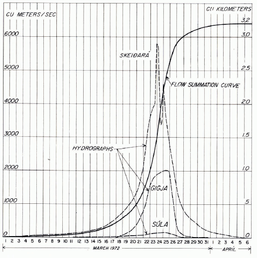
The most accurate discharge hydrograph (Q : t relation) made for a jökulhlaup from Grimsvötn is the one by Sigurjón Rist for the 1972 jökulhlaup (Reference RistRist, [1974], p. 57) which is reproduced here as Figure 6. It shows the separate discharges from the three main outlet rivers. The three discharges are summed in Figure 7 to give observed values of In Q: t which are compared with the predictions of Equation (32) with the parameters chosen to give the best fit (K 2 = 7.45X10⁻⁷m-3/4s-3/4 with the asymptote t = o at 11.00 h on 30 March). The flood falls abruptly 6.5 d before Q would be theoretically infinite.

Fig. 6. Hydrograph for the 1972 jökulhlaup. The discharges of the three main outlet rivers Skeiàarà, Gigja and Sula nre shown separately by the broken curves. Measurements by Sigurjon Rist (reproduced from fig. 3 of Reference RistRist ([1974]) by permission of the editors of Jökull).

Fig. 7. The sum of measured discharges in Figure 6 (open circles and broken curve) plotted logarithmically and compared with Equation (32) [foil curve). The close fit of the rising limb with theory is remarkable.
The excellence of the fit between observation and theory up to the flood peak is rather astonishing. Although Rist's estimated error in the observations of Q is ±20% they fit the theoretical curve to within about 4%. The plotted points were obtained (by Björnsson) from his summation of Rist's graphs and they show no observable systematic deviation from the theoretical curve only random deviations. I suggest that, while the method of observation (from a helicopter, sighting the water level in the rivers against fixed marks and measuring the geometries of the channels after the flood was over) may have given a 20% systematic error, the random errors are much smaller. In any case the agreement with the predicted analytical form gives confidence in the various simplifications that have been made in the theory. Since the index 5/4 in Equation (30) is close to 1 the Q: t relation is not far from exponential, but nevertheless very distinguishably different, as can be seen by the departure from a straight line in Figure 7. In fact a plot of In Q: In (—t) gives an exponent in Equation (32) of —4-oo±o.o6. The constant N calculated from Equation (31) is 709 m8/3 kg, which for a single tunnel of circular section corresponds to a Manning roughness coefficient n = 0.12 m-1/3s. According toReference RöthlisbergerRöthlisberger (1972, p. 181) n’ could be expected to range from about 0.01 m-1/3 s for a straight smooth pipe to 0.1 m-1/3 s for a meandering boulder-strewn torrent at the bed. Our calculated n’ lies at the rough end of the range; this is to be expected if there are several tunnels operating at once (as is observed at the outlet), and if their sections are non-circular. Moreover we have ignored the effect of the transport of the large amount of sediment and boulders.
After the main peak on 23/24 March there is a subsidiary peak which is associated with water having a different deuterium content. This suggests that, after the main outburst from Grimsvötn, some water was released from a different storage place (Björnsson, personal communication). We note that, provided this water used the same tunnels as the main flood from Grimsvötn, it makes no difference to the potential gradient or to N, and so the rising part of the Q: t curve is quite unaffected by it. The discharge up to the flood peak is determined by the potential gradient and by the growing tunnels, not by intermediate storage reservoirs.
KI can be estimated from Equation (28) as 4.91X10--2m-2/3s-1, and Equation (29) then gives the plot of In S: tshown in Figure 8.
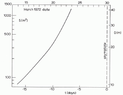
Fig. 8. Theoretical cross-section S verms time, corresponding to the theoretical Q : t curve of Figure 7. Although the main part of the theory does not assume a single circular cross-section, the scale on the right shows what its diameter D would be.
We have seen that Q during the growth stage is very nearly uniform with s, and if N were uniform we could deduce that S and dø/ds were also uniform. φ would be linear in s. But non-uniformity in N, which is affected both by roughness and by the shape of the cross-section, means that we cannot treat ø as exactly linear in s. (This is a pity, because if ø were strictly linear in s we could go on to deduce all the details p(s, t).) Figure 9 (to scale) shows a possible curve, labelled øI, for ø(s) near the start of the flood (but after the melting rate has dominated plastic contraction). The top end is fixed by the lake level LI above the position K the seal. Curve B in Figure 9 represents pwgzD(s) and may be thought of as the bed of the glacier with the height scale translated into a scale of water pressure. If we assume that the tunnel, at any rate near the top end, is at the bed of the glacier (zt - Zb), the water pressure p(s) is simply the difference between curves φI and B. We want to compare it with the ice overburden pressure pi(s), which we shall assume is pigh. Accordingly we plot pigh upwards from the bed curve B as a base, to give curve G’ (Röthlisberger's “water-equivalent line”), the actual glacier surface being G. (Before the seal was broken the potential φ followed curve G.) If G' is above φI, the ice pressure pi exceeds the water pressure p and the tunnel tends to close plastically (although of course it is enlarging very much faster by melting). But if G’ chanced to be below øI the water pressure would exceed the ice pressure, the ice would lift from the bed, the water would spread out into a sheet and the tunnel model would have broken down. At the other extreme, if the bed curve B happened to lie above øI at some place, the water pressure would be negative relative to atmospheric pressure. At a negative pressure of about I bar cavities of water vapour would form.
We have drawn øI as shown in Figure 9 hearing in mind that, with uniform N øI would be linear with s and that the end points are known. øI cannot He too far below G’; for example, if øI were drawn 20 bars below G’ in the lower part of the glacier, pi—p would be unacceptably high; the melting rate would not be enough to overcome plastic closing.
As the lake level falls curves G’ and B remain fixed, by definition, but ø(s) must fall. ø 2 shows a possible curve for ø(s) at the end of the flood. The top end is fixed by the new lake level L2 and we have simply pivoted the curve about the end point D. The construction in Figure 9 shows that the value obtained for pi—p is very insensitive to the position of the bed. Or, put in another way, the value obtained for pi—p depends very little on whether the tunnel is assumed to be at the bed of the glacier or at some higher position.
(b) How does the jökulklaup stop?
According to Björnsson's calculations the flood abates when the lake level L2 is still some 230 m above the level of the saddle point J (Figs 3and 9). At first sight this is surprising. Once the flood has started why does the lake not drain oui as far as the height of its rim will allow it? Björnsson notes that the end of the flood corresponds roughly to the moment when the lower surface of the plug of ice, 220 m thick, that floats on the lake falls to the level of J. I believe that this is a coincidence and that the flood would stop punctually as observed even if there were no ice plug on the lake. The reason is as follows.

Fig. 9. Longitudinal section of Skei∂arárjökull during the jökulklaup, to scale with vertical exaggeration x 20. The vertical scale is height translated into water pressure, B, glacier bed; a, glacier surface; G,’ water equivalent line; ø1, ø2 potentials at start and end of flood; L1,L2 lake levels at start and end of flood. Topography from Reference BjörnssonBjörnsson ([19751])
Although in our approximate calculation we have neglected the plastic contraction of the tunnel in comparison with the enlargement by melting, we can now estimate pi—p, for this is the difference between the fixed G’ curve and the changing curve for ø in Figure 9. During the flood the lake level falls 100 m. If we accept the lines drawn for ø1 and ø2 in Figure 9 the resulting increase in (pi—p) near the top of the tunnel would be of the order of 20 bars. This would represent an increase by a factor of about five. We cannot be precise about the magnitude of this factor because there are several possible complications that affect the course of the ø curves; therefore we do not insist on the fine details of Figure 9; the essential point is that the drop in lake level causes a very significant increase in the pressure difference that tends to close the tunnel. The effect is especially marked near the top of the tunnel, and it is worth noting that the collapsed cauldrons, reported by Björnsson as occurring 10 15 km below the seal, are in just this region.
If we make the very conservative assumption that the pressure difference trebles, the plastic contraction, which is proportional to the cube of the stress, increases by a factor of 27 and is now more than enough to overcome the enlargement by melting. When the two effects just balance, the flood is at its maximum. Then the tunnel contracts plastically and the flood comes to an end.
It is crucially important to notice that the effect of plastic contraction does not simply increase gradually with time as the lake level falls; on the contrary it grows extremely suddenly at the peak of the flood. There are two reasons for this. First, the fall in lake level is far from steady, If we write τ = -t, so that τ is the time remaining before the asymptote where Q = ∞ would be reached, we have seen that Q Q∝ -4 This means that, even if the lake had vertical sides so that the rate of fall of ils level was proportional to Q, its level would be given by
Zo + z∞ — Eoτ -3 ,
where Eo is a constant and z∞ is the starting value of zo at T = ∞. Second, because pi—p varies linearly with the lake level (Figure 9), it must be of the form
where P∞ and τo are constants. (It is preferable to keep a constant term in this expression, rather than having pi—p extrapolate to zero as T ∞, because, of course, the relation does not hold during the earliest part of the flood when plastic contraction may still be comparable with the melting rate.) Therefore the plastic deformation rate is proportional to
This time dependence means that the plastic deformation rate remains fairly constant and then increases very fast around τ = T 0, becoming effectively like τ -9'. The fact that the lake has sloping sides makes the increase even faster.
This very abrupt growth in the rate of plastic contraction has two consequences. On the one hand it makes it legitimate to neglect plastic contraction during the Hood and still get excellent agreement with the observed Q : t relation. On the other hand, it explains the sudden termination of the Q ∝ T -4 relation without an observable transition period.
Figure 10, which is partly calculated and partly schematic, shows strain-rate S -I [dS/dt] versus time. M is the opening rate due to melting, while P is the contraction raie due to plastic deformation. During the main part of the flood, plastic contraction being small, M may be calculated from Equation (29); this gives the surprisingly simple relation S -1[dS/dt] = 3T-I independent of K 1, shown by the full-drawn part of M. Curve p is calculated from Equation (34) by making it intersect the calculated M at the observed time of flood maximum, because here the two rates must very nearly balance. The further assumption that (pi—p) trebles during the flood fixes curve p completely. If we had assumed, instead, a fivefold or even greater increase in (pi-p) and had taken into account the slope of the lake sides, curve p would start at a lower level, would remain low for longer and would turn upwards even more suddenly to cut M at the same point.

Fig. 10. The difference between the rate of opening by melting, M, and rate of closing by plastic deformation, P, during the 1972 jökulhlaup. Full curves are calculated on the assumption that P ≪ M broken curves are diagrammatic only.
The remaining broken parts of curves M and p are diagrammatic only. We may imagine an ordinary sub-glacial drainage tunnel existing up to point w, with M and p in balance. At this time the lake rises to the critical level and M begins to exceed p. A plausible extrapolation of the calculated part of M places w on 1 March, which is the day the local people sensed a sulphurous smell at the outlet. On 13 March they were in no doubt that a jökulhlaup had started, M was now much larger than P, and it remained so until very shortly before the flood maximum at midnight on 23/24 March. The details of the curves of M and P near their intersection are not certain, because we have no solution when P is comparable with M, and we must remember the spatial variations, but we could argue as follows. At the intersection point where M = P, dS/dt = o and S is a maximum. dø/ds is decreasing and so Equation (23) suggests that Q also decreasing. Equation (24) then implies that m is decreasing. Thus the maximum of the curve M in Figure 10 occurs before the intersection point, as indicated by the broken line (the full part being calculated on the assumption that P ≪ M) Eventually both M and P fall back to their original values.
To summarize, our theoretical derivation of the Q: t relation in Figure 7 during the growth of the flood has depended essentially on the conservation of energy, and on the Gauckler-Manning formula in the form of Equation (12) with N constant. Thus the argument has not depended on assuming any particular shape of cross-section or on whether the water is in one or in several different tunnels, but it has assumed that the cross-section or cross-sections remain geometrically similar as they grow. It does not depend on there being other storage places besides Grimsvöln, provided they drain through the same tunnel system. The argument for the sharp cut-off of the flood by plastic contraction of the tunnel is equally independent of the cross-sectional shape, or of whether there is just one tunnel or several; for it simply uses the fact that the plastic contraction rate is proportional to a high power of (pi—p). This insensitivity to details makes the close agreement of theory with observation, which is startling at first sight, rather less surprising.
6. Intergranular Veins and Jökulhlaups
If the intergranular vein system in a glacier is a connected network as proposed by Reference Nye and FrankNye and Frank (1973), water, being the denser medium, will flow downwards. Viscous resistance to the flow will generate heat which will melt and tend to enlarge the veins. The realization of this led Reference LliboutryLliboutry (1971) to ask why, in that case, the whole glacier does not melt itself away in a rather short time. He suggested that the answer is that the vein system is blocked. Another answer could be that it is the limited supply of water to the vein system that prevents catastrophe. Vein flow, assuming that it does occur, and jökulhlaup flow clearly have something in common. But what is the essential difference?
As Röthlisberger has shown (1972), when water flows through a tunnel, the rate of opening by frictional melting can be balanced by the rate of closing by plastic deformation. It is also possible that this is essentially what happens with the vein system in a glacier (Reference ShreveShreve, 1972), so let us trace the consequences of such a supposition. When the “tunnel” is a vein, its cross-section has three corners of molecular sharpness; it might be held (Reference Nye and FrankNye and Frank, 1973) that these would produce virtually infinite stress concern rat ions and thus make plastic contraction possible with merely an infinitesimal underpressure. This is incorrect. Dr R. G. Oakberg (to be published) has now calculated the stress distribution that would be produced at a vein if the ice were isotropic and obeyed the Glen flow law. The stress near the vein corners is biaxially hydrostatic with no infinity, as conjectured by Reference Nye and MaeNye and Mac (1972, p. 98). This means that, for its response to externally applied stress, the triangular vein may be replaced by an equivalent tube of circular cross-section.
The differential equations for the time-dependent water (low in a vein may be written down in close analogy with those for a tunnel, Equations (16)-(20). We neglect the small pressure difference across the curved vein surface and also the effect of surface energy. We assume Poiseuille flow (with the same equivalent circular cross-section) and perfect heat transfer so that øw = øiUsing the pressure: melting-point relation døi/dp = -C, where G is a positive constant, means that the convective term in the energy Equation (19) is
Thus Equations (16)—(19) are replaced by:
Geometry and flow of ice:
Continuity:
Poiseuille flow of water:
Energy:
y = pw/σC = 0.313 is a dimensionless constant whose appearance in the energy equation represents an effect noted by Röthlisberger (1972) in connexion with flow in ice tunnels. In Equation (35) we have used the form from Reference NyeNye (1953) appropriate to a circular cross-section, A* being a constant in the Glen flow law.
With this model we can first ask how much underpressure in the vein is needed to provide enough plastic contraction lo compensate for the frictional melting. Putting ∂/∂t = o in Equation (35), substituting from Equation (38) for m and from Equation (37) for Q gives
We choose a vertical vein (gs = g) and estimate ∂ p/∂s = pig; then
For a vein of circular section 20 μιη in diameter this gives a pressure difference between ice and water (pi-p) of 0.6 bar (6 m head of water). Thus the underpressure in a vein relative to the surrounding ice is not large and for many purposes we can neglect it. But if we neglect it altogether there is nothing to prevent the vein enlarging by melting and, if had access to an unlimited supply of water, growing indefinitely large.
So plastic contraction of a vein to balance the frictional melting makes possible a steady state of the Röthlisberger type. But is the steady state stable against perturbations? The answer is yes and no. If the pressure difference between the ends of the vein is kept fixed, the steady state is unstable (as plausibly asserted byReference WhalleyWhalley (1971, p. 172) for Röthlisberger channels). But if the vein is fed from a reservoir it may be stable, as we shall see in a moment.
First we show the instability for fixed pressure by considering the thought-experiment of Figure IIa. A reservoir A, supplied with water from an inlet pipe c, is connected by a short length of ice tunnel with circular cross-section (the model vein) to another reservoir B, the tunnel being subjected to a fixed ice overburden pressure pi The slope of the tunnel is arbitrary. The object is to set up a Röthlisberger-type steady state. We do this by providing both A and B with very large capacity overflows at fixed heights, and we always maintain sufficient flow through C to ensure that the water levels remain at three heights. Thus the pressures pA and pB at the two ends of the tunnel are fixed. There will now be only one cross-sectional area S of the tunnel that will give steady conditions (pressure differences and gradients being fixed, the balance Equation (35) decides m\S, the energy Equation (38) decides Q/S, and then the Poiseuille flow Equation (37) decides S). Let the cross-section be chosen accordingly, and call it S 0. The state is now steady.

Fig. 11. Thought-experiments to test stability of a tunnel or vein which is simultaneously opening by melting and closing by plastic deformation. At the outflow end the pressure is fixed. Arrangement (a) with the inflow pressure fixed is unstable; arrangement (b) with the inflow rate fixed is stable, provided reservoir A has an area less than a critical value.
In the general non-steady state, when pressures and conduit gradients are held fixed, Equation (37) implies Q ∝ Sz and hence, by Equation (38), m oc S1. Thus in Equation (35) the contribution to ∂S/∂t from melting is proportional to S2 while the negative contribution to ∂S/∂t from plastic closing is proportional to S. The steady state occurs at the intersection point R (Fig. 12) where the contributions balance. If S > S 0, the melting rate exceeds the plastic closing rate and so the 'cross-section of the tunnel increases unstably (less water overflowing from A). Similarly if S < SSo the cross-section diminishes unstably to zero (more water overflowing from A)

Fig. 12. [dS/dt] versus S far the unstable arrangement of Figure 11a.
We can achieve stability by changing the system to Figure 11b. This arrangement is identical to that in Figure 11a except that there is no overflow pipe for reservoir A. We start with the tunnel having cross-section S0 and with the levels exactly as before—but in order to maintain these levels we have to reduce the inflow from c by the amount that formerly overflowed from A when we had the steady stale. We keep this inflow fixed. Then we have set up exactly the same steady state in the tunnel as before.
When the steady state is perturbed the level of water in A can change, and so to examine stability we must consider the combined system of reservoir and tunnel together. It is shown in Appendix A that for small disturbances the stability depends on the surface area of the reservoir A: below a certain critical area the system is stable; above this area it is unstable. (H. Röthlisberger had already surmised this behaviour and his letter to me on the question led to the calculation given in Appendix A.) The system illustrated in Figure IIa, which we have already seen to be unstable, is equivalent to having an infinite reservoir. The stability condition does not depend on there being a fixed inflow into reservoir A. The inflow represents a forcing term which merely serves to determine what steady state one has.
The differential equation for small perturbations of cross-section of the tunnel is second-order and linear. Mathematically, instability arises because the damping coefficient can be negative. At the critical reservoir area the damping is zero, and so at and around this area the system oscillates, stably or unstably. For small reservoir areas the system is over-damped and there is no oscillation. Similarly for large areas a disturbance grows unstably without oscillation. The critical area of the reservoir is very much greater than the cross-section of the tunnel or vein in all practical cases.
The analysis described is for a length of tunnel that is short enough for us to be able to regard the pressure gradient, discharge, cross-section, and the other variables as changing only in time and not in space. A study of the behaviour of spatial variations would be interesting but will not be attempted in this paper;Reference Nye and FrankNye and Frank (1973) suggest that kinematic waves will travel along a vein. However, the present analysis goes far enough to show that the stability of a tunnel or a vein in a Röthlisberger-type balance depends on the end conditions. The pressure being held fixed at the outflow end, the system is unstable when the inflow is held at fixed pressure, but stable when fed from a reservoir of small area. The latter combination is normally appropriate to a vein in a glacier. I suggest that the stability of this combined system of vein and small reservoir explains not only why veins do not normally grow catastro-phically in size, but also why they generate just the right underpressure to balance melting by Plastice contraction. This ceases to be remarkable as soon as one realizes that it is merely a consequence of the tendency to seek a stable steady state. On the other hand, feeding a tunnel from a reservoir at fixed pressure is an appropriate model for draining a large lake and the instability of this configuration is responsible for jökulhlaups. If it were not for this instability, the lake level in Grímsvötn would remain at the critical level for lifting, and the lake would simply overflow gently through a subglacial drainage system, its outflow being balanced by its inflow.
When a tunnel is growing unstably (Fig. 10) there are two stages: at first the melting rate is still comparable in magnitude with the plastic closure rate, although of course it is faster. In the second stage the melting rate is considerably faster. In Section 5a it was the second stage that we analysed in detail, because we treated the plastic closure rate as negligibly small. We have not given a detailed mathematical analysis of the first stage (which would include all the details of the variations with s), but we have identified in this section the essential feature that causes instability.
7 Veins and Ggrímsvötn
In view of the argument just given why does Grimsvötn not drain out through the inter-granular veins long before the critical level for floating is reached? After all, it is essentially a reservoir at fixed pressure.
We have already noted (Section 3) that before the seal at κ (Fig. 3) is broken a thin water sheet at the bed of the glacier up-stream from κ is driven uphill towards the lake, not away from it. It is simple to extend this argument to include the intergranular vein water as follows.
FollowingReference ShreveShreve (1972) define the potential ø = pwg (z – zo) + p,
where p is the pressure in the veins and z0 is the height of the top surface of the lake. The effective pressure gradient driving the water is then — grad ø This definition of ø is the same as Equation (2), except that it now applies to veins in the interior of the glacier rather than only to the bed, and the zero level for potential has been changed.
Neglecting the underpressure in the veins, take p as the overburden pressure of the ice at the point (x, z) in question, pig(zs — z). Then
The equipotential ø = o is
This is the curve ANC in Figure 13a, obtained by reflecting the surface of the glacier in the lake level and exaggerating the scale by a factor of 10; it is the same as curve B in Figures 2 and 3 and represents the bottom surface the ice would need to have to float in isostatic equilibrium. AF is the hypothetical bottom surface of the ice in contact with the lake. The other equipotentials in Figure 13a are obtained by simply translating the curve ø = o up and down. If the veins made the ice isotropically permeable the lines of water flow would be orthogonal to the equipotentials, but even taking account of anisotropy the only result we need is that the vein water will flow from higher to lower ø When the glacier bed is as shown, before the seal is broken, clearly the vein water is forced towards the lake.

Fig. 13. (a) Equipotentials for vein-water within the ice near an ice-dammed lake such us Grimsvötn. (b) Schematic equipotentials for vein-water when an ice-dammed lake dos not reach bedrock.
The effect of the underpressure in the veins is to reduce p, and therefore ø throughout the ice, thus lowering the potential barrier; the reduction could correspond to a few metres of water head.
8. Veins and A Lake Perched on the Ice
The foregoing analysis is readily extended to the situation of a glacier lake that does not necessarily reach bedrock. Figure 13b shows an idealized section through such a lake which has a horizontal ice bottom at zt. Because a point (x, z) may now have both ice and water above it, the vein pressure/; in Equation (41) is to be taken as the overburden pressure due to the overlying ice and any overlying water that may be present. The equipotential ø = o and those above it are the same as before. To draw the equipotentials below it we need only observe that ∂φ/∂z = (pw – pi)g in ice and ∂φ/∂z = oin water.
If water is to escape from the lake by draining through the veins, the glacier bed must be everywhere below the equipotential φ = o because otherwise with an impermeable bed there would be no path that did not cross the forbidden region ANC of higher potential, N is a critical point. In terms of ice freeboard H, if the bed is less than 10Hbelow the lake level the lake will not drain through the veins. But if the bed lies below this critical depth the lake may drain through the veins, making use of the instability appropriate to a large reservoir of fixed pressure.
It appears that this is why glacier lakes, particularly marginal lakes where the glacier depth is small, are able to exist at all in spite of the porosity provided by the vein system in the ice; and this is also why lakes in the middle of temperate glaciers, where the ice is deep, are seldom if ever seen. It is interesting to compare this explanation for marginal lakes with that given byReference ShreveShreve (1972, p. 212); as far as I can see the explanations do not conflict, although they differ in emphasis.
A lake sealed in this way can empty suddenly if forward motion of the glacier establishes a path, say a crack or crevasse, that short-circuits across the forbidden region ANC. But we must remember that the region is only forbidden because veins have time to adjust their internal pressure to be about equal to the overburden pressure—and so a pathway must be opened quickly if it is to be effective. This, rather than a change of water level, may sometimes explain the sudden emptying often observed in marginal glacier lakes.
Acknowledgements
Helgi Björnsson visited Bristol University Physics Department for two years with the. aid of a European Council Scholarship (administered by the British Council). This paper has been able to focus on the classic jökulhlaup from Grimsvotn largely because of the detailed information on the phenomenon that he has assembled (Reference BjörnssonBjörnsson, [1975])- I am most grateful to him for his congenial collaboration.
I should also like to mention the field meeting of the International Glaciological Society in Iceland in 1970, organized by Professor Sigurdur Thorarinsson, which acted as a springboard for the work. Professor C. F. Raymond and Professor H. Röthlisberger both commented very helpfully upon the manuscript.
Appendix A
The Stability Of A Vein Connected To A Reservoir
We wish to examine the stability of the system, represented in Figure 11b, of a short length of vein connecting two reservoirs, the water in the lower reservoir being maintained at a fixed level. The time-dependent equations for flow in the vein are Equations (35) to (38). Let/in be the fixed pressure at the outlet end and let pB + P(t) be the varying pressure at the inlet end. When the fixed length l of the vein is small enough we may take the pressure gradient to be uniform, p in Equation (35) is taken as the mean pressure pB + 1/2P(t), while S, m and Q are taken as the spatial means. Equation (36) merely serves to give the spatial change of discharge. The other three equations (35), (37) and (38) become
for the variables S(t), m(t), P(t), Q(t). The equation for the upper reservoir is
where α is its surface area, h* is the height of the water surface above the outlet, and Qi = Qi(t) is the inflow. The vein being short, we neglect the variation of discharge along it and take the outflow from the reservoir to be the same as the spatial mean flow Q through the vein. Since pwgh* = pB = P, the reservoir equation becomes
The four equations (A-1), (A-2), (A-3), (A-4), with known Qi and initial conditions, determine the problem. Elimination of Q and m in these four equations gives
and
as equation for S(t) and P(t). Now put

where suffix o denotes the steady state and suffix 1 denotes a small perturbation from it. Note that we perturb the inflow as well as the pressure and the cross-section.
If the term in dP/dst in Equation (A-5) is expressed in terms of P and S by using (A-6), the resulting coupled pair of perturbation equations is
where the constant coefficients A, B, C, D, E, F depend solely on the steady-state parameters, thus:

The physical meaning of Equations (A-7) and (A-8) is most clearly seen if we set y = 0 (no pressure-melting effect) instead of γ — 0.313, which is the true value. The final result. Equation (A-11), shows that y represents merely an awkward complication, having some quantitative effect on the stability condition but not making any qualitative difference. With γ = o, Equation (A-7) has F = o and comes from the physics of the vein flow, while Equation (A-8) expresses the behaviour of the reservoir drained by the vein. Thus in Equation (A-7) we may consider the case where PI is constrained 10 be zero (infinite reservoir); B is positive and represents an exponential growth constant for the cross-sectional perturbation S I This is the instability discussed in the main part of the paper in connexion with Figure 11a. On the other hand, in Equation (A-8), if Q, and S: are set equal to zero (fixed inflow and fixed cross-section for outflow), an initial perturbation in the level of the reservoir, giving an initial P Iis seen to relax exponentially, for C is negative, The essence of the behaviour of the combined system is the competition between the instability of the vein and the stability of the reservoir.
To see the physical meaning of A, note that if the system is in a steady state and the pressure is suddenly increased by P, by raising the level in the reservoir, the cross-section grows at the rate dS/dt = API Similarly for D; if the system is in a steady state and the cross-section is suddenly increased by SI, the pressure changes at the rate dPI /dt— DSI ; D is negative, indicating that the level in the reservoir will fall, as it must.
Continuing the formal analysis, if we eliminate P I in Equations (A-7) and (A-8) we obtain the following second-order linear differential equation for S I:
The terms in dQ /dt and Q I on (the right-hand side are forcing terms and do not affect the stability conditions. First we show that the coefficient S I is positive. Substitution of the expressions for A, B, C and D given by Equations (A-9) shows that the required condition is
Since all three terms are separately positive this inequality is satisfied unconditionally. Thus the coefficient of SI', in Equation (A-10) is positive, and the system is equivalent to a harmonic oscillator with a damping coefficient -(B+C).
For stability (positive damping)
B+G < o.
Substituting the values of B and G from Equations (A-9) gives
where
αc is the critical value of the reservoir area. Smaller areas give positive damping; larger areas give negative damping, and therefore instability. (If the reservoir has sloping sides, αc and αc must refer to the area of the water surface.) It is straightforward to show that for α range of a around αcthe system will oscillate if disturbed, but that there is no oscillation for very small or very large αc
To see the order of magnitude of αc take the case where the pressure gradient in the vein is the same as it would be in a mass of ice with a horizontal surface, so that P0 = -pigel Then, with gs = g sin θ, θ being the inclination of the vein, we have
Since L/g is a length (34 km) large compared with l the term in y in the numerator is negligible. Moreover one can see that the coefficient of S0 is a large number: the critical reservoir area is much larger than the vein cross-section. Table A-I shows values of αc for a vein of circular section 20 μm in diameter. As we have not considered the effect of spatial variations along the vein it is not clear what value of l is most appropriate. But the table shows that, for a very wide range of values, the critical area of the reservoir lies between the cross-sectional area of a vein and the area of a glacial lake—and this is the essential result that we need.
Table A-I. The Critical Area. αC of The Reservoir for Diffkrent Lenghts l and Inclinations θ of a Vein.

Appendix B
Differential Equations For Non-Steady Water Flow In A Basal Sheet
These equations may be written down very simply by analogy with those for a vein. As for a vein we assume perfect heat transfer and slow viscous flow, but in this case we shall also assume that the water pressure p is equal to the ice pressure pi .
Take the s coordinate in the direction of flow, let q(s, t) be the volume of water flowing per unit width per unit time, let m'(s, t) be the melting rate of mass per unit area, and let a(s, t) be the thickness of the water sheet. The equations analogous to (35)—(38) are:
Geometry:
Continuity:
Poiseuille flow of water: Energy:
Energy:
In the first equation R(s, t) which is analogous to (∂S/∂t)pI is the rate of lifting of the ice. The unknowns are q, m’, a and R but because R appears only in the first equation the system reduces essentially to three equations for three unknowns.
Appendix C
Tunnels Or A Sheet?
We have remarked that the observational evidence would allow the water during a jökulhlaup from Grimsvötn to be in a basal sheet rather than in a tunnel system for at least part of its course. Our approach has been to show that if we adopt the hypothesis that the water flows in a tunnel system it leads to no obvious contradiction. But, of course, we might have proceeded from the opposite direction and looked for a self-consistent sheet-flow solution. Without having calculated it in detail 1 believe that, if no lateral gradients are allowed in the bed or in the ice thickness, a solution would exist corresponding to a water sheet fed steadily from a top reservoir along a horizontal line at the head of the glacier and flowing down to a line sink at the end of the glacier. But for several reasons I do not think this type of solution offers a realistic alternative to the tunnel solution.
In the first place the breaking of the hydrostatic seal at the up-stream end provides a concentrated source of water rather than a line source. So to be in a sheet the water would have first to fan out. Having fanned out, assuming it did do so, it would encounter at least two effects tending to force it to concentrate in a tunnel. The first comes from the potential gradient. If we assume that the water pressure in a sheet equals the ice overburden pressure, it follows from Equation (2) that
and so
grand φ ≈ pig (0.1 grad zb + grad z s).
and so
In other words, as is well known, the surface gradient of the ice is some 10 times more effective than the bed gradient in directing the flow of water, If the surface had no lateral slope, there would thus be a weak force driving the water towards valleys in the bed; but moderate lateral surface gradients can overcome this tendency and drive the water towards valleys in the surface. In either case a sheet would tend to concentrate into channels. The fact that the two main outlet streams of Skeidarárjökull emerge the two edges of the glacier front, both in normal times and during a jökulhlaup, probably reflects this influence of the ice surface gradient. '
Another effect tending to concentrate a sheet into channels arises from the heal production. In a transverse section through a water sheet at the bed of a glacier, because the How is fastest where the sheet is thickest, these places will melt fastest, and so thickness variations in the water sheet will become accentuated. In calculating the process from the basic differential equations (B-1)-(B-4) the difficulty is to decide how to treat R, the rate of lifting of the ice. The differential equations (B-1)-(B-4) assume that processes are slow enough for the ice to move up and down differentially and plastically and so achieve the balance p = pi . For faster processes this condition will no longer be fulfilled and p becomes an unknown, but if the processes are so fast and on a small enough scale that there is no time for the ice to sag differentially we can put R = o. If we assume perfect hydraulic connexion in the transverse direction, so that the potential is the same for all points in a transverse section we then find
Thus a place twice as thick as average grows eight times faster. This seems a powerful concentrating process, but to calculate it in detail entails a closer consideration of the plastic sagging.