
It is becoming increasingly common for sociolinguists to utilize large speech corpora in their research where the data collection was conducted at multiple different periods in time. I will refer to these kinds of corpora as “multistage corpora.” With several projects devoted to collecting and curating archival recordings alongside contemporary fieldwork, this is likely to be a growing methodological trend. While invaluable for the study of language change, multistage corpora contain more complexity in their representation of time than do fieldwork data collected at a single point in time. Most traditional sociolinguistic projects have just one time dimension to measure language change against: speakers’ age. This is an overloaded measure since an age effect could easily reflect either an effect of generational cohort (an Apparent Time interpretation), or an effect of speakers’ life cycle (an Age Grading interpretation), or both (Sankoff, Reference Sankoff and Brown2006). Usually the case is made for a generational cohort or life cycle interpretation based on how the age effect interacts with other dimensions, like gender, socioeconomic class, or style. In multistage corpora, the generational cohort effect and lifecycle effect can be partially unlinked. Two speakers may have the same date of birth, but not the same age, if they were interviewed 20 years apart. Conversely, two speakers may share the same age, but not the same date of birth. A third, underdiscussed, time dimension is included in these multistage corpora: the year of recording.
This paper draws data from the Philadelphia Neighborhood Corpus (PNC), which contains sociolinguistic interviews conducted annually from 1973 to 1994, then every other year until 2012. The PNC may be unique in that all of the data was collected for the same purpose (course work for the graduate course, Ling560: Researching the Speech Community) following broadly similar procedures for the full time of collection. However, other speech corpora covering similarly broad ranges have been constructed by combining data from separate research projects that surveyed the same speech community. For example, three different waves of data collection in Tyneside by researchers affiliated with Newcastle University (Tyneside Linguistic Survey, 1960s–1970s; Phonological Variation and Change in Contemporary Spoken English, 1990s; Newcastle Electronic Corpus of Tyneside English 2, 2000s) were combined to create the Diachronic Electronic Corpus of Tyneside English ([DECTE]; Corrigan, Buchstaller, Mearns, & Moisl, Reference Corrigan, Buchstaller, Mearns and Moisl2012). The Origins of New Zealand English (ONZE) corpus was formed by incorporating archival material recorded by the New Zealand Broadcasting Service, a separate independent broadcaster, a few interviews done on an ad hoc basis, and data collected according to a regular schedule for coursework, producing a corpus of data recorded between the 1940s and the 2000s (Gordon, Maclagan, & Hay, Reference Gordon, Maclagan, Hay, Beal, Corrigan and Moisl2007). At first glance, it may seem impossible to construct a new corpus covering a time scale similar to the PNC, DECTE, or ONZE without the benefit of time travel, but there are several projects currently underway attempting to collect and curate archival recordings into similar speech corpora. One example is the Language Infrastructure Made Accessible project (Johannessen, Reference Johannessen2016), which has the goal of collecting and digitizing recordings made between the 1950s and 1980s of Norwegian dialects, Sami, and North American heritage Norwegian speakers. Another is the Gra.fo project, which is collecting and digitizing a massive number of Tuscan oral archives (Calamai, Reference Calamai2011). All indications suggest that use of corpora like these is a growing trend, so a methodological investigation into utilizing their complex time dimensions for the study of language change is urgently required.
In addition to the methodological issues involved, there is a core sociolinguistic question at stake here: to what extent is intraspeaker language change across the lifespan implicated in language change in progress? Most of what is currently understood about language change in progress has relied upon the Apparent Time construct, which assumes that speakers remain stable across their lifespans, making them effectively time capsules of the language as it was spoken at their time of acquisition. Besides the number of case and panel studies of individual speakers that have found this assumption to not be entirely true, recent developments in the theory of language change incrementation suggest that intraspeaker change is necessary for change to occur (Labov, Reference Labov2001; Tagliamonte & D'Arcy, Reference Tagliamonte and D'Arcy2009). With the mixture of time dimensions available in multistage corpora, it is possible to explore whether there is any systematicity to which speakers exhibit lifespan instability and whether this instability is linked to specific life stages.
TIME DIMENSIONS AND INTRASPEAKER CHANGE
Apparent Time and Real Time are the two time constructs most commonly utilized to study language change. The Real Time construct is utilized most commonly in historical linguistics, where the date of the text is taken to represent the state of the language at the time it was created. The Apparent Time construct is used more often to study language change in progress, where speakers’ date of birth is taken to represent the state of the language at the time they acquired it. Sankoff (Reference Sankoff and Brown2006) summarized 12 studies that utilized the Apparent Time construct to diagnose instances of language changes, which were then followed up with a later study providing a Real Time component. In almost all instances, the Real Time restudy found the change to have further incremented, lending some important credibility to the Apparent Time construct.
However, it is known that the core assumption that supports the Apparent Time construct, that speakers remain stable in their linguistic behavior after a critical period, is not absolute. Individuals who have moved from one speech community to another have been found to acquire second dialect features to some extent (Chambers, Reference Chambers1992; Nycz, Reference Nycz2013; Sankoff, Reference Sankoff and Fought2004). Isolated examples such as these may not be sufficient for general principles of language change, which must ultimately affect an entire speech community. However, cases of sustained adult-to-adult dialect contact may lead to such speech community level change. Labov (Reference Labov2007) called language change driven by dialect contact in this way diffusion, in contrast to endogenous language change, transmission. Crucially, the clear-cut cases of diffusion, such as the irregularly diffused components of the Northern Cities Shift along the St. Louis Corridor, necessarily involve a violation of the core Apparent Time assumption. By hypothesis, the Northern Cities Shift manifests as it does in St. Louis because it was acquired by adults after their critical period.
In addition to adult speakers altering their language due to dialect contact, there is increasing evidence that intraspeaker change during adolescence is part of the natural development of speakers through their life cycle and is actually a necessary process for language to change. A number of studies have found that children probability match their parents very closely in the use of linguistic variation (Labov, Reference Labov1989; Roberts, Reference Roberts1997; Smith, Durham, & Fortune Reference Smith, Durham and Fortune2007, Reference Smith, Durham and Fortune2009). However, if it were the case that children perfectly matched the input from their parents, the language would logically remain static. Instead, it has been proposed that between early childhood and early adolescence, children undergo a dialectal reorganization that has the function of incrementing language change when they overshoot the previous cohort's target. This account explains the frequently observed “adolescent peak,” where the youngest children in the speech community are actually fairly conservative with respect to a language change (Labov, Reference Labov2001; Tagliamonte & D'Arcy, Reference Tagliamonte and D'Arcy2009). This proposal complicates the analysis of the relationship between variable linguistic usage and speakers’ age. By hypothesis, the observed relationship between age and linguistic use from the youngest ages to late adolescence represents intraspeaker change, as speakers undergo this dialectal reorganization. From late adolescence onward, the relationship between age and linguistic use tends to be analyzed as representing intergenerational change.
There is also a substantial body of research utilizing panel studies, studying and restudying the speech of a panel of speakers across their lifespan (Wagner, Reference Wagner2012a). Much of this research has focused on the postadolescent transition of a small number of individuals from high school into higher education and adult life (De Decker, Reference De Decker2006; Rickford & Price, Reference Rickford and Price2013; Wagner, Reference Wagner2012b), and case studies of individuals (Carter, Reference Carter2007; Harrington, Palethorpe, & Watson, Reference Harrington, Palethorpe and Watson2000; MacKenzie, Reference MacKenzie2014). There are also a number of panel studies where a larger number of speakers were reexamined at 10- or 20-year intervals (e.g., Bowie, Reference Bowie2005; Gregerson, Maegaard, & Pharao, Reference Gregersen, Maegaard and Pharao2009; see Sankoff, Reference Sankoff, Bayley, Cameron and Lucas2013, for a broader review of these panel studies). The lifespan study with perhaps the densest sampling of panel members is Van Hofwegen and Wolfram (Reference Van Hofwegen and Wolfram2010), who analyzed the rate of African American Vernacular English use of 67 children who were interviewed at six points in time between the ages of 4 and approximately 15. They found a fair amount of volatility within these speakers across this time period. The panel study that is most closely integrated into the study of speech community level change is the corpus of Montreal French, which has found individuals undergoing lifespan change in consonantal (Sankoff & Blondeau, Reference Sankoff and Blondeau2007), vocalic (MacKenzie & Sankoff, Reference MacKenzie and Sankoff2010), and morphosyntactic variations (Wagner & Sankoff, Reference Wagner and Sankoff2011); however the majority pattern in all three of these domains was for speakers to remain stable. Sankoff (Reference Sankoff, Bayley, Cameron and Lucas2013) concluded that “people as they age register lesser differences from their earlier selves than does the community over the same time interval.”
We might conclude from this evidence that there is an inherent and worryingly unquantifiable uncertainty in identifying language change in progress. Speakers’ age is an overloaded measure for this purpose. To begin with, we must interpret age effects differently based on its own value. The relationship between age and a linguistic variable for very young ages represent intraspeaker changes, according to the adolescent peak model, while the relationship between age and the same variable for older ages represent intergenerational changes, according to the Apparent Time construct. Furthermore, the assumption that after some age (say, late adolescence) speakers remain fairly stable has been demonstrated not to be absolute in a number of cases studies showing intraspeaker volatility at a wide variety of ages.
However, multistage corpora provide us some data to partially differentiate between generational change and intraspeaker change. While most of these corpora do not include a panel of the same speakers reinterviewed at multiple points in time, they do have the important property that speakers’ date of birth and their age do not have an identity relationship. For example, some speakers born in 1950 may have been interviewed in the 1980s, when they were in their 30s, and then another group of speakers born in 1950 may have been interviewed again in the 2010s, when they were in their 60s. Stability within and between cohorts can then be assessed to see which time components contribute most to the observed data: the speakers’ generation, the speakers’ life cycle, or the time of the interview, the last of which I will call the zeitgeist here.
Previous approaches to time with multistage corpora
Some studies utilizing multistage corpora have already attempted to disambiguate among the effects of generation, lifespan, and zeitgeist quantitatively. The two reviewed here utilize data from the PNC.
In Labov, Rosenfelder, and Fruehwald (Reference Labov, Rosenfelder and Fruehwald2013), speakers’ date of birth was used as the primary temporal measure of language change. To justify this approach, the authors examined the goodness of fit for models using year of interview, speakers’ age, and speakers’ date of birth to predict the outcome of two different sound changes. Of the three different models fit for these two changes, date of birth, the measure of speakers’ generation, had the highest r 2, as shown in Table 1.
Table 1. Goodness of fit r2 values from Labov et al. (Reference Labov, Rosenfelder and Fruehwald2013)
This approach may have been sufficient to argue that there had been an intergenerational change for these vowels, but some problems exist for its generalizability as a methodological approach. To begin with, these two changes were the most linear in their trajectories. Applying this modeling approach to changes with more nonlinear trajectories would result in a worse r 2 than they may deserve. It would be trivial to complexify the model to include polynomial effects of these time dimensions, but that would open up the door to making even more analysis choices that lack clear decision criteria. For example, should a researcher choose date of birth or age as the primary time dimension when there is a similar r 2 for both, but date of birth requires a cubic polynomial fit while age only requires a squared polynomial fit? Moreover, the notion that our methodological goal is to choose one time dimensions and to set aside the others is not accurate. It is uncontroversial that all three time dimensions contribute to the observed data in some way or another, so what we should really be attempting to do is evaluate how much each dimension contributes compared to the others.
Zellou and Tamminga (Reference Zellou and Tamminga2014) took a different approach in their study of nasal coarticulation in the PNC. They subsetted the available data into a trend sample and a cohort sample. The trend sample consisted of all speakers under the age of 25 across the entire corpus. These speakers had a wide date of birth range, since some 25 year-olds were interviewed in the 1970s and some were interviewed in the 2010s. They attributed patterns within this trend sample to generational changes. The cohort sample consisted of all speakers born between 1940 and 1949. These speakers had a wide range of ages, again because of the time range of the interviews. They attributed patterns with the cohort sample to life cycle trends. Zellou and Tamminga (Reference Zellou and Tamminga2014) found a very striking pattern of generational change toward less nasal coarticulation and relatively marginal life cycle patterns.
The methodology used in this paper is very similar in principle to the one adopted by Zellou and Tamminga (Reference Zellou and Tamminga2014), but improved in some crucial ways. While the subsetting approach is reasonable for initial validation of a trend, it does have the shortcoming of discarding data that is potentially informative (e.g., data from speakers older than 25 and speakers born after 1949). Secondly, creating trend and cohort subsamples essentially discretizes a fundamentally continuous predictor, which is generally a suboptimal statistical methodology. For example, we would expect speakers born in 1949 to be more similar to speakers born in 1950 than to speakers born in 1940.
Approach adopted here
The approach in this paper is very similar to the underlying principle from Zellou and Tamminga (Reference Zellou and Tamminga2014), except I will be modeling the effect of speakers’ date of birth and year of interview simultaneously, and nonlinearly, using tensor product smooths, described in more detail in the Methods section. This approach has the two benefits of avoiding discretizing continuous data and utilizing the entire dataset for model fitting.
DATA
Data used
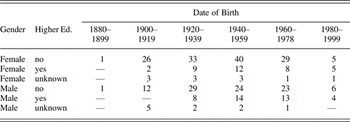
All data analyzed here is drawn from the PNC, which consists of sociolinguistic interviews carried out between 1973 and 2012, a range of 39 years. Speakers’ dates of birth range between 1889 and 1998, a range of 109 years. Speakers in the corpus are largely working class, but a consistent classification is not available for all speakers. Table 2 summarizes the demographics of the 325 white speakers from the corpus by 20-year date of birth increments, gender, and whether they have any experience with higher education (defined as years of schooling greater than 12). The median PNC interview duration is 46 min, with a 10th to 90th percentile range of 26 to 62 min. Slightly less than this was actually transcribed and analyzed (10th–50th–90th percentiles of the transcribed data are 15–30–56 min). For more information on the PNC, see Labov et al. (Reference Labov, Rosenfelder and Fruehwald2013).
Table 2. PNC demographics
All vowel formant data was automatically extracted using the FAVE suite (Rosenfelder, Fruehwald, Evanini, Seyfarth, Gorman, Prichard, & Yuan, Reference Rosenfelder, Fruehwald, Evanini, Seyfarth, Gorman, Prichard and Yuan2015). A more complete explanation of the FAVE procedures is given in Labov et al. (Reference Labov, Rosenfelder and Fruehwald2013). After force aligning a manual transcription to the audio, vowel formants are estimated using Bayesian formant tracking, excluding any tokens that have overlapping noise or speech, as well as any vowels shorter than 50 msec. The vowels reported on in this paper have specialized heuristics for choosing a measurement point. Both /ay/ and /ey/ are measured at maximum F1. Both /aw/ and /ow/ are measured midway between vowel onset and F1 maximum. The filled pause data was simply extracted from the transcriptions. The vowel formant data was z-score (Lobanov) normalized.
Changes examined
I examined five language changes in this paper: four vocalic changes and one categorical change. The four vocalic changes were previously explored in Labov et al. (Reference Labov, Rosenfelder and Fruehwald2013).
/ay0/ and /ey/
Prevoiceless /ay/ (Price as in Wells, Reference Wells1982), as in right and nice (notated as /ay0/ here) raises from a low position to a mid position over the 20th century, as reported by Labov (Reference Labov2001) and Fruehwald (Reference Fruehwald2016). Its trajectory is largely linear (Labov et al., Reference Labov, Rosenfelder and Fruehwald2013). I will be using normalized F1 as the primary measure of /ay0/ raising.
Pre-consonantal /ey/ (Face as in Wells, Reference Wells1982), as in make and same (in contrast to word final /ey/ in may and say), raises and fronts from a mid-low position to a mid-high position, partially overlapping with /iy/, resulting in a close phonetic similarity between snake and sneak (Labov, Reference Labov2001). Its trajectory is largely linear. I will be using normalized F2 – normalized F1 as the primary measure of /ey/ fronting and raising, following Labov et al. (Reference Labov, Rosenfelder and Fruehwald2013).
/aw/ and /ow/
/aw/ (Mouth as in Wells, Reference Wells1982), as in out and down, exhibits a fronting and raising trend for most of the first half of the 20th century, then slows and reverses, while /ow/ (Goat as in Wells, Reference Wells1982), as in over and most, fronts then reverses. Labov et al. (Reference Labov, Rosenfelder and Fruehwald2013) proposed that the reversal of the /aw/ and /ow/ changes, compared to the linear incrementation of the /ay0/ and /ey/ changes, is due to a larger dialectal reorientation of Philadelphia from the South to the North. I will be using normalized F2 – normalized F1 as the primary measure of /aw/ fronting and raising, and normalized F2 as the primary measure of /ow/ fronting.
Filled pauses
In this paper, I will be using “filled pauses” to refer exclusively to the fillers UH and UM. Extracts of each from the PNC are included in (1) and (2).
-
(1) She lives with her sister over, uh, around the corner.
-
(2) I'd like to stay in the city. Um, I was actually going to buy the house across the street.
These fillers are distinct compared to others in the amount of silence that follows them (Kendall, Reference Kendall2013) and have been specifically implicated in speech planning and processing (Arnold, Fagnano, & Tanenhaus, Reference Arnold, Fagnano and Tanenhaus2003; Clark & Fox Tree, Reference Clark and Fox Tree2002; Corley, MacGregor, & Donaldson, Reference Corley, MacGregor and Donaldson2007). A large cross-dialectal and cross-linguistic comparison has found that speakers are increasingly more likely to use UM when they use a filled pause (Wieling, Grieve, Bouma, Fruehwald, Coleman, & Liberman, Reference Wieling, Grieve, Bouma, Fruehwald, Coleman and Liberman2016).
METHODS
The key methodological tool of this paper is the use of tensor product smooths fit using Generalized Additive Models (GAMs) (Baayen, van Rij, de Cat, & Wood, Reference Baayen, van Rij, de Cat and Wood2016; Wieling, Nerbonne, & Baayen, Reference Wieling, Nerbonne and Baayen2011; Wood, Reference Wood2006). This method allows for fitting nonlinear, or wiggly, relationships between outcomes and predictors (e.g., vowels’ F1 and speakers’ date of birth) and nonlinear interactions between predictors (e.g., date of birth and year of interview). Allowing for such wiggly relationships between the data and time dimensions is of central importance in this paper for a number of reasons. To begin with, Labov et al. (Reference Labov, Rosenfelder and Fruehwald2013) found that /aw/ and /ow/ exhibited a nonlinear trajectory, moving in one direction for the first half of the 20th century, then reversing. Such a nonlinear trajectory could not be adequately modeled in a default linear (mixed-effects) model, since as the name implies, they can only model relationships that are straight lines between outcomes and predictors. It is possible to specify more complex (e.g., polynomial) curves in a linear model, but this is most appropriate when there is a strong theoretical motivation for a specific polynomial function, which in the case of the changes examined in this paper there is not. Moreover, by allowing wiggly relationships between the outcomes and predictors, the results are less likely to be due to our modeling assumptions. That is, if an Apparent Time trend appears, it will not be because we assumed the change was a straight line. And if there are notable lifespan or zeitgeist effects, they will be more likely to be discovered.
GAMs are very similar to smoothing spline analyses of variance, which is a popular technique for analyzing ultrasound tongue images and vowel formant tracks (Davidson, Reference Davidson2006; Nycz & Decker, Reference Nycz and De Decker2006). A key difference between the two techniques that is crucially important to the analysis presented here is that GAMs allow for modeling the nonlinear effect of two variables and a nonlinear interaction between those two variables simultaneously. Moreover, the gamm4 package in R (Wood & Scheipl, Reference Wood and Scheipl2014) also allows for the specification of random effects structures that are estimated using the familiar lme4 package (Bates, Mächler, Bolker, & Walker, Reference Bates, Mächler, Bolker and Walker2015), which I will use here to specify random intercepts for speakers and words.
To reduce the computational complexity of the models being fit, however, the data was partially summarized before models were fit. For every speaker, the relevant outcome variable (normalized F1, normalized F2, or normalized F2 – normalized F1) was averaged for each lexical item that speaker produced. For example, one speaker produced 93 tokens of prevoiceless /ay/, 53 of which were like. The average of normalized F1 for like was taken for this speaker, reducing 53 tokens to one average for the word type. This was similarly done for six tokens of fights, four tokens of nice, and so on, resulting in 18 word type averages for this speaker. This was done for all speakers, dramatically reducing the volume of data to be modeled and the complexity of the random effects structures. It is still possible to include a random intercept for word type, since many word types were produced by multiple speakers. The exception to this procedure is the modeling of filled pauses, which was given a binary coding of 0 for UH and 1 for UM.
Additionally, models were fit separately for men and women. As would be expected for most changes in progress, these changes exhibit gender differentiation. It would be possible to include gender as a predictor with an interaction with the two-dimensional tensor product smooth in a single model, but it increases the complexity of estimating the model more so than for linear models. Additionally, some attempts to fit a single model failed to converge. The consequence is that the results for men and women are not directly comparable, since they were not estimated by the same model, so the figures presenting the model results herein will all be faceted by gender.
Every model was fit with the following specification:
 $$y \sim f\left( {{\rm dob},{\rm year}} \right) + s_i + w_i $$
Where y is the outcome measure, f() is the tensor product spline function, and s i and w i are random effects for speaker and word.Footnote 1 Date of birth was chosen as a modeling dimension since this is the usual time dimension used in the Apparent Time construct. Of the remaining two time dimensions (age and year of interview), year of interview was chosen because it is less highly correlated with date of birth than age and provides a less-restricted surface across which to estimate the outcome (see Figure 1). For modeling the filled pauses data, a logistic link was used.

Figure 1. The relationship between date of birth (y-axis) and age (left) and year of interview (right). Each point represents a speaker in the data.
Both date of birth and year of interview were centered and rescaled for the purpose of modeling. Speakers’ date of birth was centered at 1940 and divided by 20, while year of interview was centered at 1993 and divided by 10. This centering and rescaling is especially important for the estimation of random intercepts. The models were intentionally kept very simple in order to maximize comparability between the changes examined and to focus them on the time dimensions of particular interest. Word frequency, for example, was not included for a number of reasons. First, it would require fitting a three-dimensional tensor product smooth instead of a two-dimensional one. This may prove to be computationally possible, but it would create analytic and expository challenges to the exploration of the time dimensions. Second, word frequency is simply not a sensible measure to include in the filled pause analysis since there are only two variants, UH and UM, being modeled. This would make the filled pause model less comparable to the other vowel shifts examined. Finally, the exclusion of word frequency should have a negligible effect on the results presented here as the word frequency effects on changes such as these tend to be exceptionally small (Dinkin, Reference Dinkin2008; Hay, Pierrehumbert, Walker, & LaShell, Reference Hay, Pierrehumbert, Walker and LaShell2015). I did not judge the benefit of marginally improved model fit against the analytic costs to be worth the inclusion of word frequency at this stage.
Once the models were fit, credible intervals were estimated using a technique called “sampling from the posterior” (see Wood [Reference Wood2006] for discussion of this method with respect to GAMs). This method can be illustrated with a simple linear regression, as in Figure 2. After fitting a model to the data, a multivariate normal probability distribution over the model parameters can be estimated. In the GAM models, the number of parameters is going to be much greater than the two parameters (intercept and slope) of the illustrative linear model, but the principle remains the same. New parameters can be sampled from this probability distribution, and the fitted values based on these sampled parameters can be calculated. A credible interval can be estimated based on these values in a number of different ways; in this paper I will be using Highest Posterior Density intervals. The illustrative example in Figure 2 draws 15 intercept and slope pairs from the posterior distribution, but for the purpose of inference in the real models fit, many more samples will be drawn. The credible intervals in all figures are based on 15,000 samples from the posterior.

Figure 2. Illustration of how credible intervals can be estimated from samples from the posterior. After a model is fit to the data (a), a multivariate probability distribution of the parameters of the model can be estimated, and samples taken from this estimate (b). The fitted values based on these sampled parameters can be used to estimate a credible interval (c).
The range of fitted values calculated was constrained to only those combinations of date of birth and year of interview that were observable in the data. For example, none of the results display the fitted value of a speaker born in 1983 and interviewed in 1973, nor a speaker born in 1900 and interviewed in 2010. This was done by assuming that only speakers between the age of 20 and 90 were interviewed in each year of fieldwork. The lower bound of age 20 means that the effect of the adolescent peak is excluded from the results and analysis. This decision was made largely because the age group of speakers who would be most actively engaged in incrementation of a sound change in their adolescence are underrepresented in the PNC.
The obvious benefit of nonlinear models is that they do not assume a strictly linear relationship between the outcome variable and the time dimensions. This is especially important for changes like /aw/ raising and /ow/ fronting, which were found to move in one direction, then reverse course over the 20th century. However, the great benefit of linear models is that there is a very simple decision procedure to determine whether there is a change in progress: test whether the effect of date of birth (i.e., the rate of change) is significantly different from 0 by calculating a p-value. The model parameters of GAMs are not similarly interpretable. Instead, what I will do to evaluate whether and when there is a reliable change across any given time dimension is to estimate the slope of a tangent line at each point along the curve for each sample from the posterior. When calculating the slope of a tangent for all points along a function, this is also known as the first derivative of that function. I will be using the forward difference of the function as an estimate for its first derivative. This is illustrated in Figure 3. For example, if we want to know whether there is a lifespan trend for speakers, we will take the fitted values from one date of birth cohort of speakers (say 1950) and take the difference between their estimated values in 1974 and 1973, then between 1975 and 1974, and so on. If we do this for every sample from the posterior, we can estimate credible intervals for the first derivative in the same way as we did for the original functions.

Figure 3. Figure illustrating locations on a nonlinear function where its tangents are (a) flat, or 0, and (b) negative. The inset illustrates how the nonlinear function is quantized (in our case over units of time such as years and ages), and how the forward difference is calculated, which will be taken as our proxy for the tangent values.
Rather than presenting a long table with p-values for every date of birth and year combination, I will instead produce graphical summaries of the credible intervals. Where these intervals exclude 0, I will conclude that there is a reliable effect.
RESULTS
The changes I analyzed will be presented according the patterns they exhibited, which fall into two broad categories. /ay0/, /aw/, and filled pauses exhibited generational stratification. /ey/ and /ow/ exhibited largely generational stratification, but both exhibit some lifespan instability as well. For /ey/, this lifespan instability is exhibited by women born after 1950, who tend to move more in the direction of the change as they age. For /ow/, this lifespan instability is exhibited by men, who move in the opposite direction of the change, but notably only during the 1980s. This appears to be a zeitgeist effect.
It should be noted that many of the figures plot trajectories for selected date of birth cohorts at 20-year intervals. This was done strictly for visualization purposes. The statistical models being visualized in these cases included all date of birth cohorts, treating date of birth as a continuous predictor, not a categorical one.
Generational stratification only
Three of the five changes examined here appear to exhibit strict generational stratification. That is, the basic Apparent Time model of language change is borne out. Speakers born more recently are more advanced with respect to the change than speakers born longer ago are. Within a given date of birth cohort, there is no, or relatively little, lifespan change.
/ay0/ modeling
Figure 4 presents the basic pattern for prevoiceless /ay/ raising in apparent time. Each point represents a speaker's mean, with a one-dimensional tensor product smooth plotted over it. Over the course of the 20th century, the nucleus of prevoiceless /ay/ raises in a nearly linear fashion. In more recent decades since the 1980s, it appears as if the raising trend has tapered off for women. Per the definition of this change, only prevoiceless tokens of /ay/ were used for modeling.

Figure 4. Basic pattern for prevoiceless /ay/ in Apparent Time.
Figure 5 plots the GAM model fits, grouped by date of birth cohort. The date to the left of each line and ribbon indicates which date of birth cohort is being plotted. The x-axis is the year of the interview, and the y-axis is the fitted normalized F1. The way to interpret the model result for women born in 1940, for example, is to follow their line and ribbon from 1973 to 2012. This line is largely flat, meaning that it does not matter whether a woman born in 1940 was interviewed in 1975, when she was 35, or in 1995, when she was 55, her prevoiceless /ay/ is probably going to be the same. This is an indicator that there is negligible lifespan change for this date of birth cohort. When estimating the rate of change within date of birth cohorts, men exhibit some spotty lifespan effects that exclude 0 in the direction opposite to the generational trend. These occasional lifespan effects are approximately half the magnitude of the generational trend and do not appear to cohere into a consistent trend, unlike the results for /ey/ and /ow/ given here. The most reliable effect here is the differences between cohorts, with the generational stratification clearly visible.
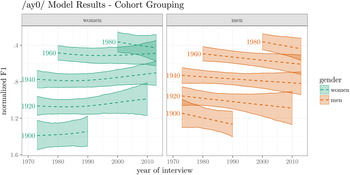
Figure 5. Prevoiceless /ay/ raising by date of birth cohort grouping. Lines represent GAM model fit, with 95% credible intervals.
/aw/ modeling
The basic pattern of /aw/ raising and fronting is slightly more complex than that of /ay0/ raising. To begin with, Labov et al. (Reference Labov, Rosenfelder and Fruehwald2013) found not only a robust gender effect, but also an influence of level of education. Speakers with at least some higher education exhibited much more marginal participation in this change. /aw/ raising also is subject to internal conditioning, where a following nasal makes it even fronter and higher (Labov, Graff, & Harris, Reference Labov, Graff, Harris and Sankoff1986; Fruehwald, Reference Fruehwald2013). These are two important components of the change worthy of further investigation in a project solely focused on /aw/. However, for the narrower focus on the time domain of change here, I will only be only analyzing the data of speakers with no higher education, and only in nonnasal contexts. The front-diagonal measure of normalized F1 – normalized F2 will be used as the outcome measure.
Figure 6 plots the basic apparent time trend for /aw/. As reported in Labov et al. (Reference Labov, Rosenfelder and Fruehwald2013), women exhibit a raising and fronting trend from the beginning of the 20th century until approximately a date of birth of 1950, at which point the trend begins to reverse. Men appear to begin participating in the change later than women and also reach the peak of the change later.

Figure 6. Basic pattern for /aw/ in Apparent Time.
Figure 7 plots the GAM model fits. Just like for /ay0/, the fitted values are plotted against the year of interview, with a fitted line and 95% credible intervals plotted for a number of date of birth cohorts. There is more considerable overlap between date of birth cohorts in this figure, partially because women born shortly after 1950 began to reverse the change. However, just like for /ay0/, there is largely consistency within date of birth cohorts. There are no date of birth cohorts who exhibit any reliable lifespan change (the credible interval of the rate of change excludes 0) at any time.

Figure 7. /aw/ raising and fronting by date of birth cohort grouping. Lines represent GAM model fit, with 95% credible intervals.
(UHM) modeling
Filled pause choice is a relatively understudied sociolinguistic variable (Acton, Reference Acton2011; Laserna, Seih, & Pennebaker, Reference Laserna, Seih and Pennebaker2014; Tottie, Reference Tottie2011), however, it appears as if there is a change in progress with UM gradually replacing UH in multiple varieties of English and other Germanic languages (Wieling et al., Reference Wieling, Grieve, Bouma, Fruehwald, Coleman and Liberman2016). Figure 8 plots the basic trend of UM replacing UH in apparent time. Each point represents each speaker's proportion of UM out of all filled pauses, and the line is the average proportion of UM per decade of apparent time.

Figure 8. Basic trend of UM replacing UH.
The modeling for (UHM) differs from the rest of the changes analyzed here in two ways. First, a logistic link was used to model the binary outcomes of UH and UM. Secondly, no preliminary aggregation was carried out. For the vocalic changes, mean values for each lexical item within each speaker were used for modeling. No equivalent aggregation could be carried out on (UHM) for modeling purposes.
Figure 9 plots the GAM model fits. The y-axis represents the logit transform of the probability of UM. As with /ay0/ and /aw/, (UHM) exhibits intergenerational change, but stability within each date of birth cohort. There are no date of birth cohorts that exhibit any reliable lifespan change at any time.
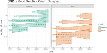
Figure 9. Increasing logit(p) of UM by date of birth cohort grouping. Lines represent GAM model fit, with 95% credible intervals.
Generational stratification and lifespan effects
Two of the changes examined here exhibited clear lifespan instability in addition to generational stratification. However, they did not do so identically. For /ey/, women born after 1950 appear to undergo additional lifespan change along with the rest of the speech community. For /ow/, older men appear to undergo lifespan change in the opposite direction from the rest of the speech community, but only during the 1980s.
/ey/ modeling
The fronting and raising of /ey/ was identified by Labov (Reference Labov2001) as a new and vigorous change in Philadelphia in the 1970s. It is a conditioned change, does not appear to be occurring before /l/ or vowels, and is significantly mitigated word-finally (Fruehwald, Reference Fruehwald2013). Here, I will only be examining nonfinal /ey/ that does not occur before vowels or /l/. Normalized F2 – Normalized F1 will be used as the outcome measure here to capture its fronting and raising.
Figure 10 plots the basic trend of /ey/ fronting and raising in apparent time. As reported by Labov et al. (Reference Labov, Rosenfelder and Fruehwald2013), this change is progressing linearly across the 20th century, with no apparent reversal trend.

Figure 10. Basic trend of /ey/ fronting and raising.
Figure 11 plots the GAM model fits, and here we find the first major divergence from strict intergenerational change. Men exhibit largely the same intergenerational stratification as for /ay0/, /aw/, and (UHM), and so do women until approximately a date of birth of 1950. In Figure 11, the 1960 and 1980 date of birth cohorts appear to be undergoing considerable lifespan change in the same direction as the speech community. It appears that a woman born in 1940 would have the same /ey/ whether they were interviewed in 1990 or 2000, but a woman born in 1960 would have a higher and fronter /ey/ in 2000 than in 1990.
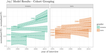
Figure 11. ey/ raising by date of birth cohort grouping. Lines represent GAM model fit, with 95% credible intervals.
A more detailed plot of this lifespan trend for women is displayed in Figure 12. The x-axis represents the year of interview, and the y-axis represents the date of birth. Every combination of date of birth and year of interview for which there is a reliable lifespan rate of change (credible interval excludes 0) is plotted. Starting with date of birth cohorts following 1950, there is a reliable lifespan trend toward greater fronting and raising. This rate of lifespan change appears to be a constant within each date of birth cohort, meaning speakers’ rate of lifespan change is constant throughout their lifespan. The lifespan rate of change appears to be greater of more recent date of birth cohorts. For example, the rate of lifespan change for women born in the 1980s is greater than for speakers born in the 1970s. The diagonal pattern across the top of the plot simply represents a gap in observable date of birth, year of interview combinations (a speaker born in 1980 could not have been interviewed in 1970).

Figure 12. Lifespan slopes reliably different from 0 for /ey/.
/ow/ modeling
/ow/ fronting is a parallel change to /aw/ fronting and raising, which has also begun to reverse in apparent time (Labov et al., Reference Labov, Rosenfelder and Fruehwald2013). Much like /aw/, it is subject to both social and linguistic conditioning. Labov et al. (Reference Labov, Rosenfelder and Fruehwald2013) found that /ow/ fronting was gender stratified, with women leading. It is also more advanced word-finally and inhibited before nasals and /l/ (Fruehwald, Reference Fruehwald2013). In order to follow the simplifying modeling approach, only nonfinal /ow/ that did not precede nasals or /l/ from speakers without any higher education was used. Normalized F2 is the measure of fronting used here.
Figure 13 plots the basic apparent time trend for /ow/. Women show a clear fronting trend that begins to flatten out around date of birth 1950. Men, on the other hand, exhibit a much more limited fronting trend in apparent time.

Figure 13. Basic pattern of /ow/ fronting in Apparent Time.
Figure 14 plots the GAM model results for /ow/. The pattern for women exhibits generational stratification like most of the other changes, with date of birth cohorts remaining relatively stable over time. Men, on the other hand, appear to exhibit an interesting mixture of generational stratification and lifespan instability. For example, the 1920s cohort appears to undergo a conservative shift away from the rest of the community until the end of the 1980s, after which they appear to remain relatively stable.

Figure 14. ow/ fronting by date of birth cohort grouping. Lines represent GAM model fit, with 95% credible intervals.
None of the female date of birth cohorts exhibited a reliable lifespan change. However, there is a strong clustering of male date of birth cohorts that have a reliably conservative movement over time. Figure 15 plots a tile for every year where a date of birth cohort has a credible interval that excludes 0. The interesting result here is that there appears to be a consistent effect across all date of birth cohorts for men to shift in the opposite direction from the rest of the speech community in the 1980s.

Figure 15. Lifespan slopes reliably different from 0 for /ow/.
One aspect of this 1980s shift, which is not easy to interpret from Figures 14 and 15, is that it does not appear as if all men are uniformly participating. Rather, the men who appear to be most actively involved in this conservative shift are middle aged or older. Figure 16 plots the predicted lifespan change for all men in 1981. It shows, for example, that in 1981, 60-year-old men were predicted to have a reliably backer /ow/ from the year before when they were 59. However, 25-year-old men are predicted to have relatively similar /ow/ backness from the year before when they were 24.

Figure 16. Predicted lifespan difference in /ow/ frontness for men between 1980 and 1981.
Importantly, the age of the men and the era are jointly important. For example, the 1940s cohort of men underwent a reliable backing trend in the 1980s, but remained stable at this backed position afterward for the remainder of their lifespan (see Figure 17 in the Appendix). Additionally, 60-year-olds only appear to have reliably backer /ow/ from when they were 59 during the 1980s. Throughout the 1990s and the 21st century, 60-year-olds appear to have relatively the same /ow/ backness as when they were 59 (see Figure 18 in the Appendix).
Lifespan effects summary
Both of these changes—/ey/ and /ow/—exhibited intergenerational change, and in fact, /ey/ for men and /ow/ for women only exhibited intergenerational change. As will be discussed further, it would difficult to say why these specific changes exhibit lifespan effects and not the others without more extensive ethnographic work, some of which may unfortunately be lost to time. Despite this, the chronological profiles of the changes have been carefully detailed and are fairly distinct from other usual Apparent Time, Age Grading, and other Lifespan Changes discussed in the literature. I have called these changes “Zeitgeist” effects, and they appear most similar to a flocking pattern, or what Labov (Reference Labov2001) labeled a “Community Change.” While some of the panel studies discussed observed lifespan changes in speakers, these patterns are typically discussed as constituting part of the natural progression of a language change (e.g., Sankoff & Blondeau, Reference Sankoff and Blondeau2007), or part of individuals’ sociolinguistic development (e.g., Rickford & Price, Reference Rickford and Price2013; Van Hofwegen & Wolfram, Reference Van Hofwegen and Wolfram2010). To my knowledge, this is the first time intragenerational change has been found to be chronologically restricted to a specific period in time.
DISCUSSION
First and foremost, these results strongly confirm that the propagation of language change in progress largely occurs through a process of intergenerational incrementation with relatively stable intragenerational patterns. Only two of the five changes examined exhibited any intragenerational, or lifespan instability, and even then only for one gender with the other gender exhibiting strict intergenerational change. This dominant pattern of intergenerational incrementation is not limited to continuous phonetic shifts of vowels. (UHM) changed in the exact same way, even though it is a categorical change with generations gradually shifting their probabilistic use of one filled pause in favor of the other. The modeling approach used here is much less restricted than other more conventionally used regression techniques, which gives patterns of intragenerational instability a greater chance of detection. The fact that the dominant pattern observed here was intragenerational stability suggests this is truly a property of language change and not an artifact of the analytic procedures commonly used in studying language change.
Accounting for which changes exhibit only generational change and which exhibit lifespan instability is not straightforward. For example, we can contrast the two cases of /ay0/ and /aw/. /ay0/ exhibits a largely linear trajectory, a marginal gender effect, and no other reliable social stratification effects. /aw/, on the other hand, exhibits a curvilinear trend, for women at least, fronting and raising at first, then reversing. It also exhibits gender differentiation, and an effect of higher education. Labov et al. (Reference Labov, Rosenfelder and Fruehwald2013) accounted for these differences by arguing that Philadelphia is undergoing a dialectal realignment from a Southern to a Northern dialect region. A raised prevoiceless /ay/ is consistent with Northern dialects, while a fronted and raised /aw/ is a more Southern feature. Further investigation is necessary, but given their different social distributions, diachronic trajectories and dialectal associations, these two changes most likely carry different socioindexial meanings within Philadelphia. However, they both appear to have incremented in the same way: strictly intergenerational shifts.
On the other hand /ey/ and /ow/ exhibited some lifespan instability even though they are largely similar to /ay0/ and /aw/, respectively. A higher and fronter /ey/ is more closely associated with Northern dialects, like a raised /ay0/, yet women born after 1950 exhibit lifespan change for /ey/ and not /ay0/. A fronted /ow/ is more closely associated with Southern dialects like a raised and fronted /aw/, yet older men in the 1980s exhibit lifespan reversal of /ow/ fronting, but now /aw/.
It appears, then, that the overall time course of the change (linear incrementation across the entire 20th century vs. incrementation and reversal) does not play a decisive role in causing lifespan instability. Difference in the way a change is socially stratified does not appear to account for the observed patterns either. For /aw/, /ow/, and (UHM), women are strongly in the lead, but only /ow/ exhibited any lifespan instability with older men retreating from the change in the 1980s. On the other hand, /ay0/ and /ey/ exhibit very little gendered differentiation in apparent time, but women born after 1950 appear to undergo significant lifespan change in the direction of the speech community for /ey/ only.
It is worth commenting on these gender effects further. In these results, I find very little evidence that the usual female lead in language change is due to lifespan change later in life (after the age of 20) for any gender. The behavior of men for /ow/ might initially appear to conform with the proposal in Labov (Reference Labov2001:308) that men retreat from female lead sound change. However, the fact that this retreat is only found in the 1980s and only for one of the three female lead changes means that this cannot be a general solution. It is suggestive that in the only two cases of lifespan instability found here women progressed further in the direction of the change and older men moved counter to the direction of the change. Further investigation into these particular changes will be necessary to understand why this should be so.
One important point to make is that strict generational stratification for a change such as /ay0/ could still be consistent with some individual speakers in the dataset undergoing idiosyncratic lifespan change. As has already been mentioned, none of the speakers in this dataset were reinterviewed, so the modeling results display the most quantitatively robust pattern within a date of birth cohort. If the dominant pattern of incrementation for /ay0/ was generational stratification with some sporadic speakers undergoing lifespan change either in the same or the opposite direction as the rest of the community, the modeling results would reflect the generational stratification with the outlying behavior of these changeable speakers relative to their cohorts being captured in the by-speaker random intercepts. Only lifespan change which reliably occurred across many speakers in the same direction at some point in time would be reflected in the modeling results. For example, Sankoff and Blondeau (Reference Sankoff and Blondeau2007) found that most of the speakers who variably used [r] and [R] in Montreal underwent some degree of lifespan change, meaning it would most likely be detected by this modeling approach. Similarly, Rickford and Price (Reference Rickford and Price2013) found some evidence of stable lifespan age grading of multiple African American Vernacular English features, which would also likely be detected by this modeling approach. Given the nonlinear nature of the modeling, if the direction of a lifespan change were to reverse for some date of birth cohort, or at some point in time, this would be captured. In summary, lifespan change must be broadly occurring in the same direction throughout the community for it to be detected using the methods in this paper.
CONCLUSION
Using a multistage corpus and nonlinear modeling methods, we have been able to decouple speakers’ age from their generational cohort in order to investigate the incrementation of language change in progress. The results show overwhelming support for the apparent time model of investigating language change: most changes are incremented between generational cohorts, and have little intragenerational instability. I also found some evidence for an effect of year of interview, a zeitgeist effect, which is often underconsidered in sociolinguistic studies. In future research utilizing multistage corpora, I recommend the use of two-dimensional tensor product smooths over the date of birth and year of interview to evaluate intragenerational stability.
APPENDIX
/ow/ figures
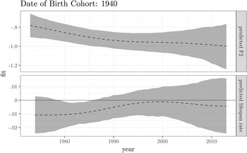
Figure 17. Lifespan trend for the male 1940 date of birth cohort. (Top) The predicted F2 for this cohort. (Bottom) The predicted rate of change in each year from the previous year.

Figure 18. Real time trend for male 60 year olds. (Top) The predicted F2 for 60 year olds in real time. (Bottom) The predicted difference from when the 60 year olds were 59.