


1. Introduction: web of belief
Quine (Reference Quine1951/1953) painted a picture of science as a web of belief:Footnote 1
“The totality of our so-called knowledge or beliefs, from the most casual matters of geography and history to the profoundest laws of atomic physics or even of pure mathematics and logic, is a man-made fabric which impinges on experience only along the edges. Or, to change the figure, total science is like a field of force, whose boundary conditions are experience. A conflict with experience at the periphery occasions readjustments in the interior of the field. Truth values have to be redistributed over some of our statements. Reevaluation of some statements entails reevaluation of others, because of their logical interconnections…” (Reference Quine1951/1953, 42)
As Skyrms and Lambert (Reference Skyrms, Karel and Weinert1995, 139) note, “however attractive this picture may be, Quine does not offer any methodology for modeling and mapping the networks of belief…”
Bayesian nets offer precisely such a model and do so in many of the respects called for by Skyrms and Lambert: “We believe that the best framework for a precise realization of these ideas is the theory of personal probability. The question then arises how to map a network of degrees of belief in a way which reveals the weak and strong resistances to disconfirmation and more generally how need for revision tends to be accommodated by the network…. Based on the conditional probability structure, notions of invariance, independence, and conditional independence all play a role in determining the place of a statement on the web of belief” (1995, 139–40).
“Webs of belief” in general, personal or cultural, scientific or non-, may take various forms, demanding various patterns of connection and updating. We don’t intend the models offered here to represent them all. We concentrate on a particular type of web, that characteristic of much of science, with emphasis on two characteristic relations—inference and confirmation. Bayesian nets, we propose, offer a particularly promising model of inference and confirmation within scientific theories.Footnote 2
Bayesian approaches to confirmation, of which there are important variations, have been widely applauded as alternatives to their 20th century predecessors in the philosophy of science, which were couched largely in classical logic (Skyrms Reference Skyrms and Rescher1987; Easwaran Reference Easwaran2011; Pettigrew Reference Pettigrew2016; Crupi Reference Crupi2020). But the success of Bayesianism contrasts with its predecessors, and debates over its variations have largely proceeded using examples of a single piece of evidence, new or old, and its impact on a single hypothesis. Here we emphasize the networks of propositions that constitute scientific theories, a theme that is central, though in relatively vague qualitative form, in a very different tradition in philosophy of science (Kuhn Reference Kuhn1962; Lakatos Reference Lakatos1968; Laudan Reference Laudan1978) and in an extensive history of conceptual maps scattered across disciplines (Axelrod Reference Axelrod and Axelrod1976; Aguilar Reference Aguilar2013; Kosko Reference Kosko1986; Papageorgiou and Stylos Reference Papageorgiou, Stylios, Pedrycz, Skowron and Kreinovich2008; Hobbs et al. Reference Hobbs, Ludsin, Knight, Ryan, Johann and Ciborowski2002; van Vliet, Kok, and Veldkamp Reference van Vliet, Kasper and Tom2010; Soler et al. Reference Soler, Kasper, Gilberto and Antoine2012; Cakmak et al. Reference Cakmak, Hasan, Ozan, Metin, Sema and Özlem2013; Jeter and Sperry Reference Jeter and Sperry2013; Homer-Dixon et al. Reference Homer-Dixon, Manjana, Mock, Tobias and Paul2014; Thagard Reference Thagard and Martinovski2015; Findlay and Thagard Reference Thagard and Martinovski2015).
Other efforts have been made to model networks of agents updating on information from other agents with various degrees of reliability or trust (Bovens and Hartmann Reference Bovens and Stephan2002, 2003; Olsson Reference Olsson and Vallinder2013; Olsson and Vallinder Reference Olsson and Zenker2013). This is again a different picture and a different target that we pursue here. Our closest predecessors are Henderson et al. (Reference Henderson, Goodman, Tenenbaum and Woodward2010) and Climenhaga (Reference Climenhaga2019, Reference Climenhagaforthcoming). The first of these is restricted to strictly linear hierarchical models of levels of abstraction with a focus on Bayesian issues of simplicity. Climenhaga represents explanatory relations between propositions as Bayesian nets in ways that complement our work here, informally in Climenhaga (Reference Climenhagaforthcoming) and more formally, but with a focus on the specific question of which probabilities determine the values of other probabilities, in Climenhaga (Reference Climenhaga2019). A more complete quantitative model of scientific theories, tracing the dynamics of evidence, implication, and confirmation percolating through branching networks of propositions, has not yet been fully drawn.
In this paper we concentrate on the structure of scientific theory and how that structure determines sensitivity to evidence impact and credence change. Evidence of a given strength can have far greater impact at one node than at another in the same structure. Webs of belief with different structures can be differentially vulnerable or resistant to the impact of evidence at a given level or the impact of a pattern of evidence over time. A study of network structure can thus reveal what Skyrms and Lambert hoped for: “the weak and strong resistances to disconfirmation” and, more generally, “how need for revision tends to be accommodated by the network.” (1995, 139–40)
Section 2 outlines a Bayesian network model of scientific theories, offering examples of the differential impact of evidence at different nodes in section 3. In section 4 those results are generalized using a graphic measure of differential evidence impact at different nodes, with an analysis through examples in section 5 of how evidence works—the interplay of network factors in the impact of evidence. To this point in the paper, for the sake of simplicity the theoretical structures considered are limited to polytrees. In section 6 the treatment is expanded to directed acyclic graphs in general. The search for generalizations regarding influential nodes in networks of various sorts is extensive across disciplines, incomplete and ongoing (Kempe, Kleinberg, and Tardos Reference Kempe, Kleinberg, Tardos, Luis Caires, Italiano, Palmedissi and Yung2005; Chen et al. Reference Chen, Hui, Lū and Zhou2013; Lawyer 2015; Bao et al. Reference Bao, Chuang, Bing-Bing and Hai-Feng2017; Li, Zhang, and Deng Reference Li, Qi and Yong2018; Champion and Elkan Reference Champion and Charles2017; Wei et al. Reference Wei, Zhisong, Guyu, Liangliang, Haiman, Xin and Zingyu2018; Hafiene, Karoui, and Romdhane Reference Hafiene, Karoui and Romdhane2019). Ours is a particular form of that search, geared to a particular kind of evidence influence in theoretical credence networks in particular.
We conclude in section 7 with further emphasis on philosophical implications of model simulations. Basic conclusions, though perhaps qualitatively intuitive, are captured here in a quantitative model open for analysis. Our attempt in the paper as a whole is to take some first steps in understanding the contribution to epistemic sensitivity and significance made by the network structure of our theories.
2. A Bayesian model of scientific theory
Bayesian networks have been developed, interpreted, and widely applied as models of causal relations between events (Pearl Reference Pearl1988, Reference Pearl2009; Spirtes, Glymour, and Scheines Reference Spirtes, Glymour and Scheines2000; Spirtes Reference Spirtes2010). But it is clear that they can equally well be taken as models of causal inference between propositions descriptive of those events—as theories. One form that scientific theories take is precisely this—a propositional representation of a causal network, between either types or tokens of events. We can therefore study structural aspects of at least one type of scientific theory by applying structural lessons from Bayesian nets.
A partial reconstruction of a causal theory for the failure of the 17th Street canal levee in New Orleans during Hurricane Katrina is shown in figure 1. A major assumption in many applications of Bayesian nets with an eye to causal inference is that all causal factors, or at least all relevant causal factors, direct or latent, are included in the representation. This is certainly not true of the reconstruction here—a partial reconstruction that captures the spirit, though not the detail, of a full causal theory.

Figure 1. A causal theory for the failure of the 17th Street canal levee in New Orleans during Hurricane Katrina. Sources: American Society of Civil Engineers Hurricane Katrina External Review Panel 2007; Bea Reference Bea2008; Rogers et al. Reference Rogers, Boutwell, Schmitz, Karadeniz, Watkins, Athanasopoulous-Zekkos and Cobos-Roa2008; Boyd Reference Boyd2012.
Lessons from causal models can also be generalized (Schaffer Reference Schaffer2016; Climenhaga Reference Climenhaga2019). The propositions within a scientific theory need not be descriptions of events, and the relations between them need not be those of causal inference. From fundamental and more general hypotheses within a theory, which might be envisaged as root nodes, multiple layers of derivative and more specific hypotheses may be inferred (Henderson et al. Reference Henderson, Goodman, Tenenbaum and Woodward2010). That inference may be probabilistic, from general grounding hypotheses to the more specific hypotheses they ground, modellable by conditional probabilities precisely as in Bayesian nets—though here our arrows represent not “x causes y” but “the credibility of y is grounded in the credibility of x” and often “x explains y.” In the other direction, evidence for more specific or applicational hypotheses can serve to confirm the more general hypotheses from which they can be inferred. This direction is often clearest in terms of disconfirmation: To what extent would x be disconfirmed were its implication y disconfirmed? Climenhaga (Reference Climenhagaforthcoming) outlines a network approach of this type informally, intended to include inference to the best explanation, enumerative induction, and analogical inference.
A partial reconstruction of a theoretical structure of this type regarding the COVID-19 pandemic is shown in figure 2. As in the causal case, a full Bayesian net representation would require all relevant grounding nodes. This is certainly not true of the reconstruction here, a partial reconstruction that captures the spirit, though not the detail, of a full theoretical structure.

Figure 2. A reconstruction of foundational theory for the COVID-19 pandemic. Sources: Kermack and McKendrick Reference Kermack and McKendrick1927; Anderson and May Reference Anderson and May1979; Hassan et al. Reference Hassan, Sheikh, Somia, Ezeh and Ali2020.
Classical 20th century models of inference and confirmation were couched largely in terms of classical logic. Bayesian models are seen as an alternative. But there is a general pattern that the two clearly share. In classical models, evidence for a hypothesis is evidence for that which it entails. In the current model, we use inference rather than entailment, cashed out in Bayesian terms of priors and conditional probabilities. In classical models, evidence for a hypothesis offers confirmation for hypotheses which entail it. Here, we take evidence for a hypothesis to offer confirmation for hypotheses from which it may be inferred, but confirmation appears in a quantitative Bayesian rather than qualitative Hempelian form. Although in accord with the spirit of classical philosophy of science, an image of scientific theories as Bayesian nets offers a far more quantitative and far more nuanced view of the basic relations of theoretical inference and evidential confirmation.Footnote 3
We model a scientific theory as a directed acyclic network.Footnote 4 Nodes represent proposition-like elements that carry credences (degrees of belief). It seems natural to speak of nodes as “beliefs,” and we will, though it is no part of our effort to defend that nomenclature literally nor to enter the debate as to what degree of credence or commitment, absolute or contextual, qualifies an item as a full “belief.” Spohn (Reference Spohn2012) emphasizes the difficulties posed by the Lottery Paradox in the latter regard. It is sufficient for the abstract purposes of our model that the nodes represent elements of a “theoretical system” or “web of belief” that carry degrees of credence or commitment. Our nodes take values in the open interval (0,1), excluding 0 and 1 themselves, though variations in this regard are also possible.
The links of our model represent the connections between the claims within a scientific theory. What is crucial is that the elements in the network are linked in such a way that credence change at one point produces credence change at the points with which it is linked. Our directed links x→y carry weights as conditional probabilities, allowing us to update both y conditional on a given credence at x and x on the basis of evidence at y. Our model networks accord with the Markhov condition: Conditional on their parents, nodes are independent of all nondescendants.
Our attempt is to model scientific networks or theoretical webs of belief as Bayesian nets, percolating credence changes at nodes through a given network structure. Some major limitations should be noted, both within this model and beyond.
Within the model, simplifying assumptions regarding conditional probability and credence assignments are noted throughout. We work with static network structures in the models explored here: Neither nodes nor links are added or subtracted. We also work with single snapshots of evidence impact; we leave to further work the promising study of dynamic network change with iterated evidence over time, including rolling changes in both node credences and conditional probabilities on links. In all these regards it must be admitted that what we offer here are merely first steps in modeling scientific theories as Bayesian nets.
Beyond this model, it must be admitted that there are probabilistic network alternatives to straight Bayesian nets, well worthy of exploration. Our hope is that the exploration of Bayesian nets in particular may motivate further work in these alternatives as well.
3. Differences in evidence impact: initial examples
We start with a simple illustration of the relative importance of differently positioned nodes in a theoretical structure. In some cases, evidence may affect just one belief or several closely related beliefs in a significant way, decaying quickly in influence across the network. In other cases, evidence of the same strength regarding another element with a scientific theory can cascade with a far stronger influence throughout the network.
Figure 3 shows a simple example of a theoretical structure modeled as a Bayesian network with credences and conditional probabilities (marked as conditional credences) in place. We offer a piece of evidence of strength [0.75, 0.25] at node y with prior credence 0.54, indicating that such a piece of evidence has a likelihood of 0.25 should y be true and a likelihood of 0.75 should y be false. On standard Bayesian conditioning, our credence at y, given that piece of evidence, changes from 0.54 to approximately 0.28:
 $${\rm{c}}\left( {{\rm{y|e}}} \right) = {{{\rm{c}}\left( {{\rm{e|y}}} \right){\rm{\times c}}\left( {\rm{y}} \right)} \over {{\rm{c}}\left( {{\rm{e|y}}} \right){\rm{\times c}}\left( {\rm{y}} \right) + {\rm{c}}\left( {{\rm{e|}}\sim {\rm{y}}} \right){\rm{\times c}}\left( {\sim {\rm{y}}} \right)}}$$
 $${\rm{c}}\left( {{\rm{y|e}}} \right) = {{0.25{\rm{\times}}0.54} \over {0.25{\rm{\times}}0.54 + 0.75{\rm{\times}}0.46}} = 0.28125$$

Figure 3. A simple Bayesian network.
But of course, a change in credence at y demands a change in credences downstream as well. Given a new credence of 0.28 at y with an indicated conditional probability of z, given y, and assuming the evidence e affects credence at z only by way of changed credence at y, our revised credence at z, given evidence e at y, changes from 0.484 to 0.587:
 $$c({\rm z|e}) = c({\rm z|y}) \times c({\rm y|e)} + c({\rm z|\sim y}) \times c(\sim \rm y|e)$$
 $$c(\rm {z|e}) = 0.3 \times 0.28 + 0.7 \times 0.72$$
by independence of z and e conditional on y.
In an extended network with the same independence assumption at each step, changes would continue downstream in the same manner.
Credence change percolates upstream as well. Using
 $${\rm{c}}\left( {{\rm{x|y}}} \right) = \;{{{\rm{c}}\left( {{\rm{y|x}}} \right){\rm{\times c}}\left( {\rm{x}} \right)} \over {{\rm{c}}\left( {\rm{y}} \right)}}$$
from Bayes with our initial priors and conditional probabilities,
 $${\rm{c}}\left( {{\rm{x|y}}} \right) = \;{{0.7\;{\rm{\times}}\;0.6} \over {0.54}} = 0.78.$$
Using
 $${\rm{c}}\left( {{\rm{x|}}\!\sim \!{\rm{y}}} \right) = \;{{{\rm{c}}\left( {\sim {\rm{y|x}}} \right){\rm{\times c}}\left( {\rm{x}} \right)} \over {{\rm{c}}\left( {\sim \!{\rm{y}}} \right)}},$$
our initial values give us
 $${\rm{c}}\left( {{\rm{x|}}\!\sim\! {\rm{y}}} \right) = \;{{0.3{\rm{\times}}0.6} \over {0.46}} = 0.39$$
Again making use of an assumption of independence, the updated credence for x, given our new value for y on evidence e at y, is
 $$c({\rm x|e}) = c{(\rm x|y}) \times c({ \rm y|e}) + c({\rm x|\!\sim \!y}) \times c(\sim \!{\rm y|e})$$
 $$c({\rm x|e}) = 0.78 \times 0.28 + 0.39 \times 0.72$$
by independence of x and e conditional on y. Thus credence at parent node x changes from 0.6 to 0.5.Footnote 5
In this picture, the direct impact of evidence on a given node ramifies one step downward to its immediate descendants and one step upward to its parents. With a screening-off assumption at each step, revised credence values for the descendants of those descendants—and parents of those parents—can be calculated in the same fashion. What we have in effect is a game of telephone, tracing revised credences percolating throughout the structure of a scientific theory.Footnote 6
We can use the absolute difference between prior and posterior credences at each node as a simple measure of credence impact at each node. Using that measure in this example, a piece of evidence of strength [0.75, 0.25] at node y has an impact of 0.26 at node y and of approximately 0.1 at the other nodes, giving a total network impact of 0.46.
Starting with the same priors, consider now evidence of the same strength at root node x instead. In that case, credence at x changes from 0.6 to 0.33, credence at y from 0.54 to 0.43, and credence at z from 0.48 to 0.526. The total network impact is 0.42. In this network with these conditional probabilities and priors, evidence impact at the central node y dominates the impact of the same evidence at the root node x.Footnote 7
A similar story holds if evidence of the same strength is delivered at node z. In that case, credence change at node z is from 0.48 to 0.23, the value of y becomes 0.637 from 0.54, and the value of x becomes 0.637 from 0.6, with a total network impact of 0.38.
Given the structure of this simple network and the patterns of belief-to-belief influence modeled by conditional probabilities and with these initial credences in place, it is the central node y that carries the most network-wide impact for a piece of evidence of the same strength.
Different network structures with different conditional links and different priors will clearly exhibit different evidence sensitivities. A second example is offered in figure 4.
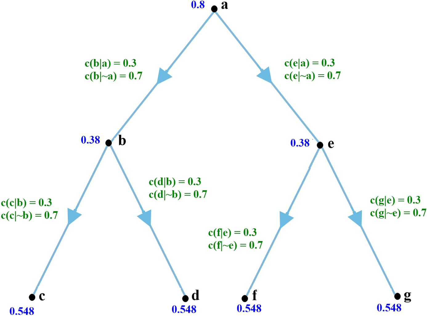
Figure 4. A second simple Bayesian network.
Initial credences and conditional probabilities are shown in the graph. With a piece of evidence of strength [0.9, 0.1] at node a—indicating a piece of evidence with a conditional probability of 0.1 if a is true, 0.9 if a is false—our credences change to 0.3 at the root node, 0.579 at each central branch, and 0.469 at the leaves; a change of 0.5 at the root node, 0.199 at the central branches, and 0.079 at the leaves. The total change for the network is 1.214, or an average change of 0.173 per node. That same strength of evidence at g gives us a total change in credences of 0.602, or an average change of 0.086 per node, less than half the change at the root. Evidence of that strength is clearly of greater impact at the top (the root) than at the bottom (the leaf).
But the situation is different if our evidence is of strength [0.1, 0.9] rather than [0.9, 0.1]. In that case the total change at the root node a is 0.418, an average change of merely 0.059 per node. Evidence of that same strength at leaf node g gives us a total change of 0.623—an average change of 0.089. Evidence with the conditional probabilities reversed thus has a roughly 50% greater impact in this network at a leaf node g than at the root node a.
What even these simple examples demonstrate is disparity in the effect of evidence, given the structure of a theoretical network, the conditional probabilities of its links, and initial priors. Given the same structure and conditional probabilities, moreover, which is the most evidentially influential node may well depend on the character of the evidence itself—in this example, [0.1, 0.9] rather than [0.9, 0.1]. At what point is a scientific theory most vulnerable to change in light of evidence? Using a Bayesian model, we have to conclude that the answer can depend on all these factors—network structure, conditional probabilities, prior credences, and the character of the evidence itself. The role that each has to play and their interaction are outlined roughly below.
4. A graphic portrait of evidence impact
What we have offered above are single-point snapshots of the differential impact of evidence of the same strength at different nodes within a network. We can envisage differential node impact more generally with graphs such as that in figure 8, illustrating impact in the network shown in figure 7.
Our graphing conventions differ from those used above. In our examples, evidence strength was indicated in terms of two conditional likelihoods [0.8, 0.1] at a node h, indicating a piece of evidence with a probability of 0.1 if h is true, or 0.8 if h is false. In fact, this is more information than is needed to determine the impact of evidence on the entire network. The ratio of these likelihoods—in this case, 1/8—fully determines evidential strength. Hence, it does not matter whether our evidence is [0.8, 0.1], [0.4, 0.05], or [0.08, 0.01]; both the immediate effect on the node in question and its overall impact on the network as a whole will be the same. Therefore, we take the likelihood ratio as a concise description of evidence strength, used on the horizontal axis of our graph in figure 5. A log scale is used to illustrate the symmetry between what we can think of as positive evidence, with likelihood ratios in (1, ∞), and negative evidence, with likelihood ratios in (0,1). We choose base 2 somewhat arbitrarily.

Figure 5. Node-averaged Kullback-Leibler divergence for evidence strength (in terms of exponent of likelihood ratio) at different nodes of the network in figure 4.
We used a simple total of changes across a network and the average change per node in our calculations above. A more elegant measure of network change is Kullback-Leibler divergence, a relative entropy measure given by:
 $${D_{KL}}\left( {p,q} \right)\;: = \sum\limits_{i = 1}^n p \left( {{A_i}} \right) \cdot \log (p\left( {{A_i}} \right){\rm{|}}q\left( {{A_i}} \right))$$
where p and q denote probability measures and A i are the propositions over which these measures are defined. Kullback-Leibler divergence gives the difference between probability measures in terms of a sum of products; namely, the product of the probability of A i according to p and the log of the probability of A i according to p, conditional on the probability of A i according to q. It can thus be interpreted as the expected logarithmic difference between distributions p and q, with the expectation taken according to p. Kullback-Leibler divergence averaged over nodes is taken as our measure on the y axis in figure 5.
The graph is read in terms of the Kullback-Leibler divergence across the entire network for evidence of a specific strength at marked nodes. On the right side of the graph a piece of evidence with strength ratio of 23 or 8/1 at node a, for example, results in a Kullbach-Leibler divergence for the network as a whole of approximately 0.03. A piece of evidence of that same strength at nodes c, d, f, or g results in a Kullback-Leibler divergence of approximately 0.07 for the network as a whole. The network impact of evidence of that strength at nodes b or e is approximately 0.13. On the left side of the graph, a piece of evidence with strength 2−3 or 1/8 has a Kullback-Leibler network impact of 0.07 at nodes b and e; 0.09 at nodes c, d, f, or g; and approximately 0.14 at root node a.
An alternative measure for network change, less familiar in some formal disciplines but more common in the philosophical literature, is Brier divergence, proportional to a squared Euclidean distance measure (Joyce Reference Joyce2009; Pettigrew Reference Pettigrew2016). The difference between prior and posterior probability distributions is taken to be the mean of the squared difference between the prior and posterior probability attached to each proposition in the network. Formally:
 $${D_{Brier}}\left( {p,q} \right)\;: = {1 \over n}\sum\limits_{i = 1}^n {{{\left( {p\left( {{A_i}} \right) - q\left( {{A_i}} \right)} \right)}^2}} $$
Results for Brier divergence, read in the same manner, are shown in figure 6.

Figure 6. Node-averaged Brier divergence for evidence strength (in terms of exponent of likelihood ratio) at different nodes of the network in figure 4.
Kullback-Leibler divergence is a measure of probability distance between the distributions of individual nodes, averaged in figure 5 to obtain a divergence metric for the network as a whole. Brier divergence is defined over a set of nodes, so it naturally serves as a network divergence metric.Footnote 8
These more complete graphical analyses underscore the conclusions drawn above, that epistemic impact across a network of evidence at a node z can depend on both z’s place in the network and on the character of the evidence, gauged in terms of its likelihood ratio— the probability, given that proposition z is true, over its probability, given that proposition z is false. In this network with these priors, the strongest impact for evidence more likely if a node’s value is false is at the root node. The strongest impact for evidence more likely if a node’s value is true is at the central nodes of the network. Evidence at the leaf tips within these parameters for evidence of either character falls in between.
We can draw two clear, though simple, conclusions on the basis of the work to this point, pursued further in the details of section 5.
The first conclusion is that in this case, as in network studies in general, the impact of evidence at a node depends on the position of that node within the theoretical structure. That is clear “vertically” from the graphs in figures 5 and 6, for example: Values at any point above or below an exponent of 0 vary with node position.
A second conclusion, in contrast to other network studies, is that the Bayesian structure of these networks is crucially important. This is clear “horizontally” from the graphs in figures 5 and 6. Any network measure that fails to incorporate the crucial factor of the character of impact at a node, in terms of likelihood ratio, will fail to identify the most epistemically influential nodes. That impact changes quite dramatically from the left to the right of graphs such as those in figures 5 and 6, though the network structure, all conditional probabilities, and all priors remain the same.
5. How evidence works: interactive factors in scientific networks
Results like those found in section 4 offer the prospect of being able to gauge epistemically sensitive nodes within the structure of a scientific theory—those elements at which evidence of a particular character would have a particular impact in terms of credence change across the network as a whole and those points at which a scientific theory would be most evidence-sensitive to change. Establishing precisely how evidence impacts a theoretical network, however, quickly becomes a challenging task.
There has been a disciplinary widespread search, for various purposes—social, technological, and epidemiological—for principles governing most influential nodes within a network (Kempe, Kleinberg, and Tardos Reference Kempe, Kleinberg, Tardos, Luis Caires, Italiano, Palmedissi and Yung2005; Chen et al. Reference Chen, Hui, Lū and Zhou2013; Bao et al. Reference Bao, Chuang, Bing-Bing and Hai-Feng2017; Li, Zhang, and Deng Reference Li, Qi and Yong2018; Champion and Elkan Reference Champion and Charles2017; Wei et al. Reference Wei, Zhisong, Guyu, Liangliang, Haiman, Xin and Zingyu2018; Hafiene, Karoui, and Romdhane Reference Hafiene, Karoui and Romdhane2019). Essentially all of this work, however, has been on networks far simpler than the Bayesian models we envisage here—on undirected networks without weighted links, for example. To the extent that consensus has emerged on network measures for most influential nodes—a consensus is far from complete—those measures will also prove too simple for Bayesian models.
Vulnerability and robustness of network structures have been studied in terms of the removal of nodes in undirected networks with applied examples such as circumstantial mechanical failures within electrical grids, evolutionary impact on specific species within an ecosystem, and terrorist attacks on airline or internet hubs (Albert, Jeong, and Barabási Reference Albert, Hawoong and Albert-László2000; Newman Reference Newman2010). For removal of nodes at random, it is scale-free and preferential attachment networks—those with a small proportion of highly connected “hubs”—that prove the most resilient against attack. Random removal is most likely to hit something other than a hub, doing relatively little damage. These are also the most vulnerable networks for targeted attacks, however, such as deliberate acts of informed sabotage—removal of a few carefully chosen hubs can do a great deal of damage. We can certainly expect something like a hub effect in our Bayesian networks. In a downward direction, credence change in nodes with more children can to that extent be expected to have an effect on a wider number of nodes and thus a more pronounced effect on the network as a whole. But here the character of that effect and its extent must also take into account the conditional probabilities on links to child nodes, not merely the existence of a link, and the character of evidence at the parent node, not merely its removal. Upward change to a parental hub node from its children must include the complication of its priors.
Eigenvector centrality and its variants (e.g., Katz centrality and PageRank) appear to be the primary candidates for measures of “most influential node” in networks far simpler than those envisaged here, despite a number of critical studies (Borgatti and Everett Reference Borgetti and Martin2006; Newman Reference Newman2010; da Silva, Vianna, and da Fontoura Costa Reference da Silva, Vianna and Costa2012; Chen et al. Reference Chen, Hui, Lū and Zhou2013; Dablander and Hine Reference Dablander and Max2019). But at their best these too are most appropriate for undirected networks modeling something like infection dynamics or directed networks modeling something like internet searches. They count transitive numbers of contacts, but don’t include the complexities of prior credences, conditional probabilities, and the likelihood ratios of evidence that are an inherent part of change within epistemic networks.
We can analyze some of the complexities involved, working toward general rules of thumb for epistemic impact, by considering three simple networks. Figure 4, considered above, has the structure of a binary tree. We represent its structure alone in figure 7 (center). The binary tree can be thought of as a structure intermediate between two others—a purely linear network, shown in figure 7 (left), and a hub or “star,” shown in figure 7 (right).
The binary tree may represent a theoretical structure in which a fundamental theory a supports two derivative theories b and e independently, each of which supports two further hypotheses. The purely linear network exaggerates the vertical descent of such a structure—a unary “tree”—in which a fundamental theory supports a derivative theory at b, supporting a hypothesis at c, which in turn supports a hypothesis at d. One can think of the hub or star figure as exaggerating the horizontal spread within a theory. Here, a single fundamental theory supports directly subsidiary hypotheses at b, c, and so forth. These, then, are differences in overall network structure. Within those structures our Kullbach-Leibler and Brier divergence graphs show the network impact at different nodes of evidence across the range of likelihood ratios. We can further consider variations in prior credences and conditional probabilities. We will emphasize Brier divergence simply because of its conceptual simplicity and greater familiarity in the philosophical literature.
For purposes of the rough rules of thumb we aim for here, we can think of a credence as high if it is greater than 0.5 (corresponding to a greater probability that it is true than that it is false) and as low if it is less than 0.5. In line with the exponents on our x axes, we can think of evidence with a likelihood ratio >1 as positive, and evidence with a likelihood ratio <1 as negative. Negative evidence in the case of a hypothesis with low credence, like positive evidence in the case of a hypothesis with high credence, we will term “credence-reinforcing” or, simply, “reinforcing” regarding the current credence. The opposite we will term “credence-counter” or, simply, “counterevidence.”Footnote 9 Finally, we can think of a pair of conditional probabilities (y|x) and (y|∼x) as positive if (y|x) > 0.5 and (y|∼x) < 0.5 and as negative if (y|x) < 0.5 and (y|∼x) > 0.5. Here we consider only symmetrical conditional probabilities, such that (y|x) and (y|∼x) sum to 1, and use the same conditional probabilities on all links. These are particularly severe limitations in this first exploration of such a model; we start with them merely for the sake of simplicity.
The simplest case of our three examples, though illustrative of some general principles that hold throughout, is the hub or star of figure 7. Figures 8A and 8B show the case in which conditional probabilities are positive throughout (uniformly [0.3, 0.7]), and our root node is given a high value of 0.6 on the left and a low of 0.4 on the right with derivative high credences of 0.54 for all other nodes on the left and a low of 0.46 on the right.

Figure 7. Three basic networks: linear, binary tree, and hub or star.

Figure 8. Brier divergence at different likelihood ratios for introduced evidence in the star network with positive conditional probabilities [0.3, 0.7] and priors of 0.6 and 0.54 (A) and 0.4 and 0.46 (B) at root and leaf nodes.
The clear left–right reversal of the two graphs follows a simple pattern that holds throughout the examples we give, not only because the priors of 0.6 and 0.4 that we use as examples are symmetrical around 0.5, but because of the assumption noted that our conditional probabilities for y|x and y|∼x sum to 1. Both of these assumptions are made simply for the sake of simplicity in exposition. Varying either of these modeling assumptions breaks the symmetry shown.
The fact that values are higher on the left in figure 8A and on the right in figure 8B follows simple Bayesian principles. We offer figure 9 as a reminder of the differential impact of evidence e gauged in terms of likelihood ratio contingent on the prior for a hypothesis, h.

Figure 9. A reminder of the immediate Bayesian impact of evidence at a node, in terms of likelihood ratio, depending on its prior.
A high prior, given evidence with what we’ve termed a positive likelihood ratio (>1), leaves us with a high posterior credence, but our posterior plummets sharply as the likelihood ratio declines and turns negative. A low prior, given evidence with a negative likelihood ratio (<1), leaves us with a low posterior, but that posterior climbs sharply as the likelihood ratio climbs and turns positive. With the conditional probabilities in place in this case, that effect carries through our example network as a whole. In figure 8A our credences for all nodes are high (>0.5), with the result that positive evidence on the right side of the graph produces a lesser impact than does negative evidence on the left. In figure 8B all credences are symmetrically low (<0.5), explaining the reverse pattern.
In the case illustrated in figure 8, regardless of whether evidence is positive or negative, it is the root node, a, that is the most influential. With this network, these conditional probabilities, and these priors, it is uniformly credence change at the root that has the greatest impact. That changes, however, if our conditional probabilities are changed from positive to negative in our rough sense, from [0.3, 0.7] to [0.7, 0.3]—from probabilities (y|x) of 0.7 and (y|∼x) of 0.3 for a node y and its parent x to probabilities (y|x) of 0.3 and (y|∼x) of 0.7. With a prior of 0.6 at node a, priors for our leaf nodes are 0.46 in this case, giving us the Brier divergence graphs of figure 10.

Figure 10. Brier divergence at different likelihood ratios for introduced evidence in the star network with positive conditional probabilities [0.7, 0.3] and priors of 0.6 and 0.46 (A) and 0.4 and 0.54 (B) at root and leaf nodes.
The reversal in our two graphs is the same as before. The fact that our root node has a higher impact than leaf nodes in the case of negative evidence in figure 10A, but lower in the case of positive evidence, is explained by the disparity in our priors. The prior for our root node is high; that for our leaf nodes is low. In this case, negative evidence constitutes counterevidence for node a while reinforcing credences in the leaf nodes, resulting in a higher credence change for the former than the latter, here reflected in changes in the network as a whole. Positive evidence, on the other hand, will be counterevidence for our leaf nodes while reinforcing evidence for our root node, reflected in the reversal of effects from the left to the right side of figure 10A. A mirror-image explanation applies for the mirror image graph of figure 10B.
The interactive factors of priors, conditional probabilities, and evidence likelihood play out along similar lines but with different effects in the different structures of our other sample networks. Figures 11A and 11B show Brier divergence in a binary tree structure with priors set at 0.6 (figure 11A) and 0.4 (figure 11B) and with negative conditional probabilities of [0.7, 0.3].

Figure 11. Brier divergence at different likelihood ratios for introduced evidence in the binary tree network with negative conditional probabilities [0.7, 0.3]. (A) A root node prior of 0.6 at node a entails credences of 0.54 at central branch nodes and 0.516 at leaves. (B) A root node of 0.4 entails credences of 0.46 at central branch nodes and 0.484 at leaves.
Here, the pattern is similar to that analyzed in section 4. For negative evidence in the case of figure 11A, it is the root node that has the greatest influence, followed by the central nodes and finally the leaf nodes. This is what one might expect from the same evidence impact at nodes with descending high priors. For positive evidence, in contrast, it is the central nodes b and c that have the most influence, followed by the leaf nodes and finally by the root. Here secondary effects of updating through the network dominate the simple effect of evidence at impact nodes.
Figures 12A and 12B show Brier divergence with the same binary tree structure and priors, but in which conditional probabilities are set at [0.7, 0.3] throughout instead of [0.3, 0.7].

Figure 12. Brier divergence at different likelihood ratios for introduced evidence in the binary tree network with positive conditional probabilities [0.3, 0.7]. (A) A root node prior of 0.6 at node a entails credences of 0.46 at central branch nodes and 0.516 at leaves. (B) A root node of 0.4 entails credences of 0.54 at central branch nodes and 0.484 at leaves.
The role of positive evidence in the case of figure 12A and of negative evidence in the case of figure 12B follows the same pattern as in the case of reversed conditional probabilities in figures 11A and 11B. The difference in conditional probabilities makes a clear difference on the other sides of the graphs. In the case of negative evidence in figure 12A and positive evidence in figure 12B the change in conditional probabilities collapses the impact of central and leaf nodes. Here evidence at the root node has a high impact, with evidence at all other nodes effectively the same, roughly as in the case of the star.
Of our three basic network structures, it is perhaps surprising that a simple linear network proves to be the most complex. Figures 13A and 13B show graphs of Brier divergence for the purely linear network of figure 7 where conditional probabilities are again set uniformly at a positive [0.3, 0.7]. In figure 13A a root node initiated at 0.6 gives us descending credences of 0.54, 0.516, 0.5064, 0.50256, 0.501024, and 0.50041 at nodes b through g. In figure 13B a root node of 0.4 gives us descending credences of 0.4, 0.46, 0.484, 0.493, 0.497, 0.498, and 0.49959.

Figure 13. Brier divergence at different likelihood ratios for introduced evidence in the linear network with positive conditional probabilities [0.3, 0.7]. (A) A root node prior of 0.6 at node a entails descending credences of 0.54, 0.516, 0.5064, 0.50256, 0.501024, and 0.50041 at nodes b through g. (B) A root node prior of 0.4 entails descending credences of 0.4, 0.46, 0.484, 0.4936, 0.49744, 0.498976, and 0.49959 at nodes b through g. Color version available as an online enhancement.
Basic principles noted above still apply: Our exploration of symmetrical priors with an assumption of conditional probabilities that add to 1 still dictates a mirror symmetry between the two cases, and counterevidence in our sense will have a greater impact on credence change in a node than will reinforcing evidence. But the pattern does not show a simple descent in overall node influence in terms of either descending network order or diminishing prior credence (in the case of figure 13A) or increasing prior credence (in the case of figure 13B). The fact that evidence at node a has the highest impact in counterevidence cases and the lowest in credence-reinforcing cases may be credited to its relatively high prior credence. But the fact that evidence at node b with the second highest prior shows the lowest impact of all nodes in counterevidence cases and the highest in credence-reinforcing cases calls for an explanation that includes node position in the network and the asymmetrical strength of upward influence through conditioning, which is sensitive to the priors of upwardly influenced nodes, and downward influence through our conditional probabilities, which is not sensitive to downstream priors. In each case those asymmetrical effects are magnified by the transitive effects through successive nodes.
The situation becomes still more complex when our conditional probabilities are set at [0.7, 0.3] instead of [0.3, 0.7], shown in figure 14 for root node priors of 0.6 and 0.4.

Figure 14. Brier divergence at different likelihood ratios for introduced evidence in the linear network with negative conditional probabilities [0.7, 0.3]. (A) A root node prior of 0.6 at node a entails descending credences of 0.46, 0.516, 0.4936, 0.50256, 0.498976, and 0.50041 for nodes b through g. (B) A root node of 0.4 entails descending credences of 0.54, 0.484, 0.5064, 0.49744, 0.501024, and 0.49959. Color version available as an online enhancement.
Here, unlike in the preceding cases, our priors are neither all high (>0.5) nor all low (<0.5). Evidence with the same likelihood ratio will therefore affect different nodes differently. Upward transfer by conditioning, moreover, will be differently affected by the differently high or low credences of nodes through which it proceeds.
The variety of effects in even these simple structures with differently positive or negative evidence, conditional probabilities, and high or low initial priors offer some hints toward the form that a network metric for evidence influence in theoretical networks would have to take. It is clear that influence metrics appropriate to the simple contact networks that have been studied, directed or undirected—without node credences, without differential evidence characteristics, and without link complexities of conditional probabilities and the complexities of Bayesian updating and conditionalization—will be inadequate here. Development of a Bayesian net analogue to eigenvector centrality that includes these factors seems a promising, if forbidding, prospect, but is beyond the scope of our work here.
6. Theoretical structures beyond polytrees
In work to this point, for the sake of simplicity we have concentrated on polytrees—structures in which each node has a single parent. Things becomes more complex when we expand consideration—as we should—to the wider range of directed acyclic graphs in general. Both of our initial examples—the causal structure of the failure of the 17th Street levee in New Orleans and the grounding structure of the theory regarding the COVID-19 pandemic—include not merely branches but downward junctures or “colliders” from multiple nodes as well as branches, well beyond simple polytrees.
Figure 15 shows the simplest downward juncture, in which credence for c is determined by values for both a and b. The simple conditional credences used above must be replaced with a conditional probability matrix, reflecting values for c contingent on combinatory values for a and b. Figure 16 shows Brier divergence for a case in which we start with a credence of 0.6 at both a and b and in which our matrix is “or-like,” specifying a value for c of 0.9 if either a or b is true and a value of 0.1 otherwise. Figure 17 shows Brier divergence for the same values at a and b but a conditional matrix that is “and-like,” specifying a value of 0.9 for c only if both a and b are true and a value of 0.1 otherwise.

Figure 15. A simple downward juncture.

Figure 16. Brier divergence at different likelihood ratios for introduced evidence in a simple “or-like” juncture with conditional probabilities [0.1, 0.9] for all cases except a = 0 and b = 0, where conditional probabilities are [0.9, 0.1]. Root node priors of 0.6 at both a and b entail a prior credence of 0.772 for c.

Figure 17. Brier divergence at different likelihood ratios for introduced evidence in a simple “and-like” juncture with conditional probabilities [0.9, 0.1] for all cases except a = 1 and b = 1, where conditional probabilities are [0.1, 0.9]. Root node priors of 0.6 at both a and b entail a prior credence of 0.338 for c.
With the same priors at root nodes and conditional probabilities of 0.1 and 0.9, the difference between “and-like” and “or-like” junctures is clear even in the priors entailed for the juncture node c—a positive 0.772 in the case of an “or-like” juncture, 0.338 in the case of “and.” The result is a reversal of evidence importance at nodes: The sensitivity of c dominates that of a and b with negative evidence in the case of an “or” juncture, while both a and b dominate c with negative evidence in the case of “and.” Appropriately to their status as duals, the cases are reversed for positive evidence.
We have already noted the complexity of evidence impact contingent on theoretical structure, priors, and conditional probabilities in the case of polytrees. Expansion to full directed acyclic graphs increases that complexity significantly even with the simple “and-like” and “or-like” junctures illustrated, let alone for the far richer palette of possible probability distributions.
The tools outlined do offer us greater prospects for understanding the parameters of evidence impact in different theoretical structures, however. As a final illustration, while fully recognizing its limitations, we offer a Brier divergence graph for the COVID-19 graph with which we began (figure 18). We use the formal treatment outlined in section 5, which builds in independence assumptions that are undoubtedly unrealistic. Full specifications for our largely ad hoc assignments of priors and conditional probabilities in this case are documented in the Appendix.

It is perhaps not surprising that the theoretical structure exhibited for the coronavirus is most sensitive to negative or counterevidence, which appears on the left side of the graph, at or near the root nodes. Were we to find out that our basic assumptions regarding germ theory, the susceptible–infected–recovery (SIR) model, or composition of viruses were incorrect our credence in the other propositions in the theory would be importantly impacted. On the right side of the graph, it is perhaps more surprising that positive or credence-reinforcing evidence most affects the graph with confirmation that handwashing stops the spread of COVID-19. It is perhaps less surprising that confirmation that SARS-CoV-2 causes COVID-19 strongly strengthens credence in other elements of the theoretical structure. As detailed in the Appendix, however, there is by no means a simple inversion in node order with regard to evidence impact from the left to the right side of the graph. Evidence regarding an R0 for the coronavirus, for example, appears relatively high on both the left and the right side of the graph, in the eighth and fifth places, respectively.
7. Conclusion
The structure of scientific theories can be modeled as Bayesian nets with values at nodes modeling credence in different propositions in the structure and conditional probabilities modeling the inferential and evidential connections between elements of the theory. Precisely because of that structure, a scientific theory will be more vulnerable to the impact of evidence of the same strength at different nodes, modeled in terms of the Bayesian impact of evidence of a particular likelihood ratio at that node.
This conclusion has two clear epistemic implications, both of which are probably intuitive, but both of which are captured here in a quantitative model.
The first implication is that relative position of different nodes within a single theoretical structure can make a major epistemic difference. Given a single theoretical structure, evidence impact at one point in a structure will have a different effect on credences, percolated through the network, than will evidence impact at another point. Calculating the network factors that lead to greater influence, however, is far from simple, depending not merely on the skeletal structure of a network but on the specific conditional probabilities on inferential and evidential links, the specific prior credences within the network, and the likelihood-ratio character of the evidence itself.
The second and related implication is that the differences between different theoretical structures can make a major epistemic difference. The same piece of evidence at the leaf node of a star-like network will have an importantly different effect than at the leaf node of a linear network, or a binary tree. Here again, however, calculating the aspects of theoretical structure that make the difference in evidence impact in different cases proves to be far from simple.
These are first steps; we have emphasized the preliminary and suggestive character of our work throughout. The promise of an approach to scientific theories as Bayesian nets is the promise of being better able to understand the theoretical–structure–relative dynamics of scientific evidence and scientific change. Fulfilling that promise will demand development of a more complete understanding of node-importance centrality in Bayesian nets, further modeling of dynamic change within Bayesian nets with iterated credence changes, and modeling of structural changes in the theoretical structures themselves. That is where some of the questions of greatest interest lie, but all of that we leave to further work.
Appendix
Specifications of root node priors and conditional probabilities for sensitivity calculations in the reconstruction of the COVID-19 theoretical structure shown in section 7.
Nodes:
-
a = germ theory
-
b = transmission
-
c = Koch
-
d = causes COVID-19
-
e = respiratory infection
-
f = airborne and contact
-
g = proximate human contact
-
h = social distancing
-
I = coronavirus composition
-
j = SARS-CoV-2 is coronavirus
-
k = breaking lipid
-
l = soap and water
-
m = handwashing coronaviruses
-
n = handwashing SARS-CoV-2
-
o = handwashing COVID-19
-
p = SIR
-
q = Kermack-McKendrick
-
r = R0
-
s = COVID-19 R0 1.4–2.0
-
t = extremely contagious
-
u = sigmoid curve
-
v = levelling off
-
w = acquired immunity
-
x = COVID-19 extinction
Root nodes a, c, I, j, and p—prior credences of 0.8. Nodes l, f, a, w—prior credences of 0.7.
Conditional probabilities:
-
p(b|a) = 0.8; p(b|∼a) = 0.2
-
p(d|b, c) = 0.8; = 0.2 otherwise
-
p(e|d, f) = 0.8; p(e|d,∼f) = 0.5; p(e|∼d, f) = 0.5; p(e|∼d, ∼f) = 0.2
-
p(g|f) = 0.8; p(g|∼f) = 0.2
-
p(h|g) = 0.8; p(h|∼g) = 0.4
-
p(k|i) = 0.7; p(k|∼i) = 0.2
-
p(m|l, k) = 0.8; p(m|l,∼k) = 0.5; p(m|∼l,k) = 0.5; p(m|∼l,∼k) = 0.2
-
p(n|m,j) = 0.8; p(n|m,∼j) = 0.5; p(n|∼m,j) = 0.5; p(n|∼m,∼j) = 0.2
-
p(o|d.n) = 0.8; = 0.2 otherwise
-
p(q|p) = 0.8; p(q|∼p) = 0.2
-
p(r|q) = 0.8; p(r|∼q) = 0.2
-
p(u|q) = 0.8; p(u|∼q) = 0.2
-
p(t|r,s) = 0.8; 0.2 otherwise
-
p(v|u) = 0.8; p(v|∼u) = 0.5
-
p(x|j,d,w,v) = 0.9; p(x|∼j,d,w,v) = 0.8; p(x|j,∼d,w,v) = 0.8; p(x|∼j,∼d,w,v) = 0.7; p(x|j,d,∼w,v) = 0.8; p(x|∼j,d,∼w,v) = 0.7;
-
p(x|j, ∼d,∼w,v) = 0.7; p(x|∼j,∼d,∼w,v) = 0.6; p(x|j,d,w,∼v) = 0.8; p(x|∼j,d,w,∼v) = 0.7; p(x|j,∼d,w,∼v) = 0.7; p(x|∼j,∼d,w,∼v) = 0.6; p(x|j,d,∼w,∼v) = 0.7;
-
p(x|∼j, d,∼w,∼v) = 0.6; p(x|j,∼d,∼w,∼v) = 0.6; p(x|∼j,∼d,∼w,∼v) = 0.2
Brier divergence scores by node for evidence likelihood 2−5, left side of figure 21:
-
0.032702925196386255 p SIR
-
0.03197274586977256 q Kermack-McKendrick
-
0.02892300064134992 a germ theory
-
0.025206021616052884 I coronavirus composition
-
0.023849404607912673 c Koch
-
0.023530107955275256 b transmission
-
0.021985716054253094 j SARS-CoV-2 is coronavirus
-
0.021732855368419703 r R0
-
0.020731908792273795 u sigmoid curve
-
0.02050306150659843 x COVID-19 extinction
-
0.018859774335903478 s COVID-19 R0 1.4
-
0.01876352205497495 v levelling off
-
0.018291007460366212 l soap and water
-
0.018142736120275237 f airborne and contact
-
0.01684255830020106 w acquired immunity
-
0.01577183852380332 m handwashing coronaviruses
-
0.015542370861284812 k breaking lipid
-
0.015403295972751313 n handwashing SARS-CoV-2
-
0.0153470017407081 d causes COVID-19
-
0.015074719685156309 h social distancing
-
0.013945521086314742 e respiratory infection
-
0.01066307009488828 g proximate contact
-
0.01028733771960207 t extremely contagious
-
0.006463834532320453 o handwashing COVID-19
Brier divergence scores by node for evidence likelihood 25, right side of figure 21:
-
0.01664743806591248 o handwashing COVID-19
-
0.01439930691393785 t extremely contagious
-
0.012583132032143445 d causes COVID-19
-
0.010663070094888275 g proximate contact
-
0.009542603689210295 r R0
-
0.009103101547024603 u sigmoid curve
-
0.008347243506501229 e respiratory infection
-
0.007966962560939319 m handwashing coronaviruses
-
0.007820365918820486 q Kermack-McKendrick
-
0.0072646504369333125 k breaking lipid
-
0.007046065875329723 h social distancing
-
0.006301081627599784 n handwashing SARS-CoV-2
-
0.005755340972874356 b transmission
-
0.004496778986033397 v levelling off
-
0.0038829270106076202 s COVID-19 R0 1.4
-
0.003765826974073341 l soap and water
-
0.0037353002678103607 f airborne and contact
-
0.003467614372621885 w acquired immunity
-
0.002546901691876484 p SIR
-
0.0022525214128471527 a germ theory
-
0.002231827418619689 x COVID-19 extinction
-
0.001963043327588758 I coronavirus composition
-
0.0018573900830391689 c Koch
-
0.0017122461394334491 j SARS-CoV-2 is coronavirus


 Open access