


1 Introduction
Under the current practice of benefit-cost analysis (BCA), the direct economic benefits produced by a newly built transit facility are assessed based on how it affects travel time and various costs that are associated with transport needs and travel behavior (Marleau Donais et al., Reference Marleau Donais, Abi-Zeid, Waygood and Lavoie2019). Savings on travel time and cost typically form the largest share of project economic benefits, and comparing the forecast ridership against the observed becomes a primary standard when judging the accuracy of a transport project evaluation. However, copious literature and research have certified that in many cases the actual number of users is below projections, and this phenomenon is particularly severe in the case of public transport projects (Mackinder & Evans, Reference Mackinder and Evans1981; Pickrell, Reference Pickrell1989; Flyvbjerg et al., Reference Flyvbjerg, Skamris holm and Buhl2003; Bain & Polakovic, Reference Bain and Polakovic2005; Flyvbjerg, Reference Flyvbjerg2007; Voulgaris, Reference Voulgaris2019). Given such results, the time-saving-based benefit calculation approach has been questioned and criticized.
Significant positive changes in the value of land where transport enhancement is proposed or completed have long been observed (Garrison et al., Reference Garrison, Berry, Marble, Nystuen and Morrill1959). Mohring (Reference Mohring1961) categorized this kind of value increment as “nonuser benefits,” since the extent to which the land value appreciates is independent from the degree to which the land owners rely on the transport facilities. He further explained that only by adding those gains to the benefits generated by the direct usage of existing and new transport facilities, without double counting, can the overall distribution of total economic benefits brought by the transport enhancement be precisely examined (Mohring, Reference Mohring1961, Reference Mohring1993).
Accessibility, the measure of the ease of reaching valued potential destinations, has been widely applied as a metric to describe transport system, and its strong correlation with land value has been repeatedly observed and attested (Dewees, Reference Dewees1976; Lin & Hwang, Reference Lin and Hwang2004; Hess & Almeida, Reference Hess and Almeida2007; Agostini & Palmucci, Reference Agostini and Palmucci2008; Dubé et al., Reference Dubé, Thériault and Des Rosiers2013; Riekkinen et al., Reference Hiironen, Riekkinen and Tuominen2015; Sun et al., Reference Sun, Wang and Li2016; Wen et al., Reference Wen, Gui, Tian, Xiao and Fang2018; Levinson & Wu, Reference Levinson and Wu2020). These findings introduce an opportunity to gauge the economic value of a transport project by estimating the change of value of residential real estate.
In this paper, we hypothesize that unlike the traditional perspective of quantifying travel time and cost savings, the change in the value of real estate better captures the economic impact of transport services more quickly, directly, and properly. Using the Second Avenue Subway in New York City as an example, we intend to validate the hypothesis by answering the following questions. First, how does the actual travel time saving (TTS) compare with the original forecast? Second, how does the change in access by transit caused by the Second Avenue Subway influence residential real estate prices and rents in surrounding neighborhoods? Third, how much is the appreciation in residential property value due to the announcement of the Second Avenue Subway and that due to the opening of the Second Avenue Subway? Fourth, how do the measures of residential property value and rent compare with actual and forecast TTSs, and with project costs? Last, was the Second Avenue Subway worthwhile?
This paper flows as follows: the intrinsic flaws of time-saving-based approach and the advantages of access-based assessment are outlined in Section 2. The Second Avenue Subway is introduced in Section 3. Section 4 briefs data and quantitative models used to address the correlation between house price and various explanatory variables. The resulting real estate hedonic models are presented in Section 5. The calculation methods of appreciation in residential property value are specified in Section 6. Finally, a comparison of the numeric results output by access-based and time-saving approach is performed in Section 7, and the implication of the access-based approach on value capture strategy is discussed in Section 8.
2 Travel time savings vs. access for benefit-cost analysis
Under the current practice of BCA, savings on time and various costs associated with transport needs and travel behavior form the main body of the direct economic benefit of transport project (Marleau Donais et al., Reference Marleau Donais, Abi-Zeid, Waygood and Lavoie2019). In the Draft Environmental Impact Statement (DEIS) for the Second Avenue Subway project, about 70 % of social and consumer benefits are linked to TTSs, including travel time reduction from the perspective of transit commuters and auto users (The Metropolitan Transportation Authority, 1999). However, the time-saving-based benefit calculation approach has been questioned for several intrinsic flaws.
First, the bottom-up evaluation approach applied to aggregate project benefits only considers what can be accurately quantified and reliably measured, overlooking those unquantifiable benefits even if they are important (Nash, Reference Nash and O’Flaherty1997; Beria et al., Reference Beria, Maltese and Mariotti2012). TTS benefits seemingly intuitively sketch out how the proposed project would achieve transport-related objectives, which is typically the predominant gains evaluated when assessing the feasibility of transportation investment (Beesley, Reference Beesley1965). However, land use-related gains, which would have been supposed to be a key benefit but are perhaps less predictable and measurable (certainly they are not direct outputs of transport models, and are typically outside the domain of transport modelers), are generally swept off in the quantitative BCA analysis and thus fail to contribute during project prioritization and selection (Wang et al., Reference Wang, Zhong and Hunt2019).
Second, the direct project benefit, with travel time- and cost-related gains being the representatives, cannot fully describe the actual economic benefit generated by the prospective project, as while it captures use, it does not capture option value. Nevertheless, Beria et al. (Reference Beria, Giove and Miele2012)) show that the examination on how accessibility has been improved is either vaguely conveyed in the calculation of changes in user’s surplus or assigned to wider economic benefit assessment in qualitative manner.
Last, labeling intangible resources (time) and human feelings (level of comfort) with an arbitrary price is recognized as a congenital defect for the traditional BCA. Although the rationale underlying such monetization processes is logical from the traditional rational planning approach, the consideration paid for acquiring those intangible benefits is not credibly quantified because there is no market trading them and no prices are quoted (Ackerman & Heinzerling, Reference Ackerman and Heinzerling2002). As a result, Ackerman and Heinzerling (Reference Ackerman and Heinzerling2002) insist that the unit dollar value of those benefits is determined under official guidance that is primarily extracted from past experience on comparable projects, but suffers from a lack of attention to project-specific characteristics. For example, when evaluating the Second Avenue Subway, the baseline unit value of TTSs is set to be equal to the average hourly rate in New York Metropolitan area under FTA 5309 guidance (The Metropolitan Transportation Authority, 1999). However, how travelers value travel time reduction varies with income (Lisco, Reference Lisco1967). The prevailing hourly rate in Manhattan which the Second Avenue Subway serves is higher than the average hourly rate across New York (U.S. Census Bureau, 2017a). The proportion of high-income groups is also higher in Manhattan, so the unit value of travel time assigned to this group of people should also be higher (U.S. Census Bureau, 2017b).
Recognizing the aforementioned defects inherent in the time-saving-based and cost-saving-based BCA approach, we propose the access-based land value benefit assessment as an alternative. The primary principle of the access-based method is that the economic value of a transport project’s intangible gains, including both TTSs and comfort, as well as their option value, is largely capitalized by nearby properties’ value appreciation, which is directly caused by improved transport accessibility.
The general applicability and wide acknowledgement of accessibility form the first advantage of access-based assessment method. Access (or accessibility) is an indicator of the level of development of transportation network. After decades of research, the definition and calculation method of access (or accessibility) are ample and diversified, but a consensus has been sustained that it measures the ease of reaching (or being reached by) designated opportunities from a particular origin (Hansen, Reference Hansen1959; Committee of the Transport Access Manual, 2020). Furthermore, the ultimate value created by an advanced transportation system is enhancing accessibility to desired places instead of reducing travel time by speeding up trips (Levine et al., Reference Levine, Grengs and Merlin2019).
The positive correlation between land value and accessibility to manifold activities has been attested and observed over and over again. Hansen (Reference Hansen1959) addressed that the possibility of being intensively developed is higher for regions with better access. Wegener (Reference Wegener, Hensher and Button2004) accentuated that the interplay between travel behavior and location choice facilitates that transport planning needs to synchronize with land utilization planning, which lays foundation for American urban planning in recent decades. Brigham (Reference Brigham1965) pointed out that the value of a piece of land is jointly determined by its access, comfort level, geographical features, and other unquantifiable factors. He further specifies that, among houses that are in equal proximity to city center, those with better access are more expensive. For instance, Dubé et al. (Reference Dubé, Thériault and Des Rosiers2013) found that the new transit service in Montreal’s South Shore created location advantages for properties close to transit stations, resulting in value appreciation in those properties.
The second superiority of access-based method lies in that the measures (accessibility and house price) it used for assessment are more inclusive and insightful than those used in time-saving method. As described previously, accessibility is a comprehensive measure covering concerns on time, distance, and trip purpose (Páez et al., Reference Parkes, Kearns and Atkinson2012). Horner (Reference Horner2004) deems job accessibility to be a leading factor influencing buyers’ residential property choice. Decisions on property choice are generally made after synthesizing people’s willingness to pay for numerous activity and rights (Kim & Horner, Reference Kim and Horner2003), so property price is remarkably informative. Concerns about travel time, expenses, and distance for trips have been well encompassed and reflected in house purchasing decision (Fierro et al., Reference Fierro, Fullerton and Donjuan-Callejo2009; Mohd Thas Thaker & Chandra Sakaran, Reference Mohd Thas Thaker and Chandra Sakaran2016). Apart from that, concerns on qualitative factors, such as natural environment (Hörnsten & Fredman, Reference Hörnsten and Fredman2000; Tan, Reference Tan2012) and the quality of adjacent neighborhoods (Rohe & Stewart, Reference Rohe and Stewart1996; Parkes et al., Reference Páez, Scott and Morency2002; Kim et al., Reference Kim, Horner and Marans2005; Caudill et al., Reference Caudill, Affuso and Yang2015), cannot be quantitatively captured by the time-saving method, but can be precisely included in house price and thus grasped by the access-based approach.
Unlike the value of travel time which is arbitrarily and subjectively decided, the market value of real estate can be easily ascertained through online databases. Benefitting from the demand-supply relationship and fierce competition in real estate market, property price is an objective indicator, and the price data are open and transparent (Adair et al., Reference Adair, Berry and McGreal1996). In addition, house price data can be acquired at little to no cost and updated whenever it needs.
Many researchers have perceived and exemplified the impact of transport infrastructure or policies on housing prices (Dewees, Reference Dewees1976; Lin & Hwang, Reference Lin and Hwang2004; Hess & Almeida, Reference Hess and Almeida2007; Agostini & Palmucci, Reference Agostini and Palmucci2008; Riekkinen et al., Reference Hiironen, Riekkinen and Tuominen2015; Sun et al., Reference Sun, Wang and Li2016; Wen et al., Reference Wen, Gui, Tian, Xiao and Fang2018; Costa et al., Reference Costa, Ramos and Zheng2021), and some of them have taken this opportunity to approximate property value appreciation and weigh against project cost (Gu & Zheng, Reference Gu and Zheng2010). However, we notice two limitations.
First, their measures of access are inconsistent and confused with the measures of distance. They set up independent variables representing the effect of a transport project, regress them on housing price, and judge the magnitude of impact on housing price based on the coefficient output by the regression model. However, their accessibility variable is virtually various distance (network distance (Dewees, Reference Dewees1976; Lewis-Workman & Brod, Reference Lewis-Workman and Brod1997) or straight-line distance (Chen et al., Reference Chen, Rufolo and Dueker1998; Bowes & Ihlanfeldt, Reference Bowes and Ihlanfeldt2001; Lin & Hwang, Reference Lin and Hwang2004; Hess & Almeida, Reference Hess and Almeida2007; Gu & Zheng, Reference Gu and Zheng2010; Riekkinen et al., Reference Hiironen, Riekkinen and Tuominen2015; Sun et al., Reference Sun, Wang and Li2016) to designated destinations which are generally city center or the closest transit station, which is at best a poor surrogate for measures of actual number of opportunities. Second, they stop by either observing the tendency as to how housing price has shifted before and after the delivery of a new transport project, or imprecisely estimating property value appreciation by multiplying the total market value of affected properties and the coefficient (Gu & Zheng, Reference Gu and Zheng2010).
We thus decide to improve on these existing efforts by aggregating housing value increment by property type, discounting the total appreciation back to present value and weighing this value against total project cost, which would enable the computation of cost effectiveness measurements like net present value (NPV) and benefit-cost ratio (BCR).
3 An introduction to the Second Avenue Subway
From the end of the nineteenth century to the beginning of the twentieth century, one subway line (Lexington Avenue Subway Line) and two elevated train lines (along Sixth and Ninth Avenue and Second and Third Avenue) operated across East Manhattan and were responsible for passenger transportation. In 1920s, the two elevated train line services were gradually ceased because of filthy street condition, outmoded infrastructure and equipment, underserved travel demand, and expensive maintenance and renovation cost (Valk, Reference Valk2016).
Since the cessation of elevated train lines, the construction of residential properties and commercial buildings in Upper East Side and Midtown East were still in full swing. The Lexington Avenue Subway, as the only rail service traversing East Manhattan, was incapable to cope with the growing demand for travel and commute (The Metropolitan Transportation Authority, 1999). As a result, the vision of a subway beneath Second Avenue, which could replace the elevated train lines and share the travel burden of Lexington Avenue Subway, had been ongoing since the 1920s. However, the construction of this subway has been repeatedly postponed due to events like the 1930’s Great Depression, World War II, the Vietnam War, and the 1970’s financial crisis (Plotch, Reference Plotch2015).
In 1999, the official publication of DEIS symbolized that the construction of the Second Avenue Subway was being reconsidered. In DEIS, apart from the baseline “No-Build Option,” 3 out of the 11 “Build Options” entered into the final quantitative and engineering analysis stage. The transportation systems management (TSM) alternative featured low expense and attempted to relieve travel pressure by reducing the time headway of Lexington Avenue Subway and adding two new bus lanes serving between 96th Street and the Lower East Side. Alternative 1 proposed constructing five new stations and a new subway (Second Avenue Subway) operating between 65th Street and 125th Street and continue using the existing Broadway line to the south of 63rd Street. Alternative 2 differs with Alternative 1 by replacing the Broadway Subway line with a new light rail service. Alternative 1 was approved to be the locally preferred alternative project option, and the construction of the Second Avenue Subway was separated into Phases 1 and 2 (The Metropolitan Transportation Authority, 2004, 2018). In the Final Environmental Impact Statement (The Metropolitan Transportation Authority, 2004), the full-length Second Avenue Subway (including Phases 1 and 2) was proposed to be an independent subway line extending 13.7 km from 125th Street in East Harlem to Financial District in Lower Manhattan (as shown in Figure 1). Phase 1 started construction in 2007 and was delivered in 2017, and Phase 2 is still in the planning stage (The Metropolitan Transportation Authority, 2020a). However, the construction and operation time of the Second Avenue Subway to the south of 63rd Street has not been specified yet.

Figure 1. The Second Avenue Subway and selected neighborhoods in Manhattan.
4 Data and methodology
4.1 Time-saving-based assessment
We intend to test the accuracy and efficiency of the TTS method by comparing the computed actual time savings against the estimate reported in the Second Avenue Subway DEIS. In the DEIS, in contrast with the “No-Build” option, each project alternative impacts traffic mobility, individual travel behavior, system capacity, and access to transit facilities to varying degrees. As a result, the expected project benefit for each project alternative is gauged primarily based on how travel demand and travel time differ from the “No-Build” option. Those quantifiable project benefits are subdivided into five major groups: (i) TTSs, (ii) reduced peak-period subway crowding, (iii) reduced off-peak standing passengers, (iv) reduced nonrecurring subway delays, and (v) reduced auto and taxi travel. We focus on the change in transit person TTS, which forms part of the first benefit group and occupies more than 70 % of total project benefit.
In order to compute the actual transit user TTS after project opening, we need the actual transit travel time, observed ridership, monetized value per unit of TTS, and a calculation model to synthesize them together. Google Maps is used to measure actual travel time. Since the Second Avenue Subway Phase 1 launched three new stations, we extract three actual travel time for each trip departing from one of the three new stations and destined to one of the six busy subway stations in Manhattan including Grand Central Terminal, Times Square (42nd Street), Chelsea (23rd Street), New York University (NYU) Medical Center, Battery Park City (in West Lower Manhattan), and Wall Street Station (in East Financial District). The origin-destination pairs are the same as those reported in the DEIS. The first actual travel time forces the travel route along or at least partly along the new subway line. The other two are the minimum and maximum actual travel time for alternative travel routes that do not use the Second Avenue Subway, which aims at mimicking the “no-build” scenario. Then the actual TTS is calculated as the actual travel time along the new subway line minus the average of the minimum and maximum travel time for alternative routes. Observed ridership is exported from Average Weekday Subway Ridership on the MTA (The Metropolitan Transportation Authority, 2020b). Abiding by FTA Section 5309, the unit monetization value of TTS is equivalent to a percentage of average wage rate in metropolitan area. The average hourly rate of $20.30 was adopted in calculating expected project benefit in DEIS, so we stick with this value but adjust for inflation. However, we lack access to the calculation model that was used in the adopted in DEIS and cannot directly output the monetized total transit person TTS. As a result, we can only compare if the TTS and ridership differ between the actual and forecast conditions.
4.2 Access-based assessment
The kernel of access-based assessment lies in the correlation between real estate value (the explained variable) and explanatory variables covering property attributes and changes of transport condition. This correlation is generally measured with hedonic regression analysis (Sheppard, Reference Sheppard, Cheshire and Mills1999).
The first step is to collect housing price. The real estate studied in this paper comprising residential market includes both rental and sold residential properties, although a portion of sold properties contain a mixture of residential and commercial units. We thus do not include the uplift (or loss in value) associated with commercial properties in the study area. We expect this means we are underestimating the gains associated with the project. Housing price data are exported from a database released by New York Department of Finance. Data for sold property are provided by Annualized Sales Update (The NYC Department of Finance, 2021a) and rental property information are offered by Cooperative/Condominium Comparable Rental Income Archives (The NYC Department of Finance, 2021b).
Then two major factors were considered when choosing regression models analyzing how the Second Avenue Subway affects price and accessibility of residential properties in adjacent neighborhoods. The first factor is time in the infrastructure timeline. The impact of the new subway on property sold price emerges far earlier than that on rental properties. This is because that a buyer would expect house value appreciation immediately after the official announcement of subway construction, but a tenant would not realize any benefit until the opening of the new subway. Since the Second Avenue Subway began construction in 2007 and opened in 2017, the study time window for sold property is 2006–2018 and that for rental property is 2016–2018. After removing $0 sales and properties with missing or problematic information, a total of 3770 properties sold through 2006–2018 were selected. However, the job accessibility data provided by the Accessibility Observatory at the University of Minnesota were unavailable before 2014 (Accessibility Observatory at the University of Minnesota, 2020). Only 1943 (51.54 % of 3770 observations) properties sold during 2014–2018 were remained. In addition, 1458 rental condominiums and cooperatives with 3 year rental history (2016–2018) provide a total of 4371 observations, which makes up the data frame for rental properties.
The second factor is whether we have repeat observations on the same property over years. We have information on the same rental properties across three years, whereas we have different sold properties across five years. As a result, the rental property dataset forms a balanced panel dataset where the rental price and other property attributes are available for the same property every year from 2016 to 2018, and a panel regression model is applied. The sold property dataset is essentially a cross-sectional dataset which consists of different sold properties in each year, and a hedonic pricing model is engaged.
After selecting the regression model, variables set-up for regression analysis has been outlined in Table 1. The fourth variable: access to jobs by transit ( $ t $
) from a property location (
$ t $
) from a property location ( $ n $
) within 30 min (30) (
$ n $
) within 30 min (30) ( $ {A}_{n,t,30} $
), which is available for each year from 2014 to 2018, is designated as a transport proxy to illustrate the impact of the Second Avenue Subway.
$ {A}_{n,t,30} $
), which is available for each year from 2014 to 2018, is designated as a transport proxy to illustrate the impact of the Second Avenue Subway.
Table 1. Variable names and descriptions.

a The symbol ✓ denotes that this variable is applicable for sold property.
Job accessibility by other transport modes like auto or walking is dropped because the data are inconclusive. Variables 7 and 8, and 13 and 14 are used as dummy variables to further classify sold and rental properties, respectively. Variable 9 is a dummy variable that distinguishes whether a property is sold before (2014–2017) or after (2018) the opening of the new subway. However, for rental properties, year dummy variable is set up for each year (as shown by Variable 15), with year 2016 being the base year. Variables 16–19 denote the neighborhood of the sold (rental) property. Among the three new subway stations delivered as part of Second Avenue Subway Phase 1, two of them are constructed in Upper East Side and one in East Harlem. The second phase of the Second Avenue Subway will primarily be deployed in Midtown East, South of Upper East Side. No other new subway line has been planned or constructed in recent decades in Upper West Side (King, Reference King2011). We designated Upper East Side to be the base group, which allows the observation of different intercepts for each neighborhood in the model and thus compare the uptrend of housing prices by zone.
5 Analysis results
5.1 Time-saving analysis
Table 2 summarizes the travel time saving analysis for the Second Avenue Subway. The 50 year accumulated transit person TTS accounts for more than 70 % of 50 year accumulated customer and social benefits for Alternatives 1 and 2. The weight of this benefit item is far lower in the TSM alternative because no new rail service was planned under this option.
Table 2. Comparison of project benefit cost results.

Note: We modified this table based on the original table sourced from the DEIS established by The Metropolitan Transportation Authority (1999)
Abbreviations: DEIS, Draft Environmental Impact Statement; TSM, transportation systems management.
a In line with the analysis method applied MTA in preparation for DEIS, the discount rate is 2.65 %.
b The base year applied when discounting project cost and benefits to present value is the year of construction begin, which is 2004 for alternatives in DEIS and 2007 for Actual(2018). Furthermore, a 50 year forecast horizon is taken when accumulate the present value for customer and social benefits.
c The annual TTS is estimated based on the fully operation of the entire Second Avenue Subway in 2020, while, in fact, only Phase 1 was opened before 2020.
d EH stands for East Harlem, and UES denotes Upper East Side. Second Avenue Subway Phase 1 primarily locates in these two neighborhoods.
e This is the AM peak hour transit TTS per trip that originates from stations in East Harlem and Upper East Side.
f This percentage denotes the 2018 actual annual ridership and transit TTS per trip as a percentage of the estimated ones in Alternative 1.
When switching the focus to the annual patronage departing from stations in East Harlem and Upper East Side, the goal of serving 40 million users per annum (in Alternative 1) has been missed. The actual number of travelers boarding the Second Avenue Subway from new stations in those two neighborhoods was 24.06 million in 2018 (59.85 % of the anticipated 40.2 million passengers).
In addition, in terms of the TTS per trip, the objective of reducing the average AM peak hour transit travel time per trip (including both in-vehicle and out-of-vehicle travel time) by 4.8 min was missed for these stations. Grounded on the real-time AM peak hour travel time extracted from Google Maps (as per Table 3), the actual transit TTS per trip is 1.83 min, accounting for only 32 % of the expected 5.73 min for the same station pairs. The TTS for trips heading to NYU Medical Center is negative, implying that traveling via the Second Avenue Subway extends the travel time. This is because travelers have to select M15 between 110th St and 96th St, and M34 bus service between 63rd St and the NYU Medical Center.
Table 3. Average travel time savings per trip AM peak hour (minutes).

Notes: TTSs per trip under alternative project options are extracted from DEIS, which were reported in integers. Actual TTSs per trip and the average TTSs per trip are calculated by us, so the results were rounded to one decimal place. DEIS assumes Phases 1 and 2 of the Second Avenue Subway built. Actual TTSs are based only on Phase 1.
Abbreviations: DEIS, Draft Environmental Impact Statement; NYU, New York University; TSM, transportation systems management; TTS, travel time saving.
The estimated TTS was projected for the to-be-completed 6 km northern Second Avenue Subway Line, so the actual transit patronage might hit the target after the opening of the second phase. However, the TTS for trips heading to South Manhattan (Times Square, Chelsea, and Financial District) may not be significantly improved until the operation of full-length Second Avenue Subway, including succeeding phases connecting to Hanover Square in South Manhattan.
5.2 Rental properties
The descriptive statistics for rental properties are displayed in Table 4, and the distribution of rental price per square meter is displayed in Figures 2 and 3. The results of panel pooling regression models for rental properties are outlined as per Table 5.
Table 4. Descriptive statistics for rental properties (2016–2018): N = 4371.


Figure 2. Frequency distribution of rental price per square meter by year (N = 4371).

Figure 3. Frequency distribution of rental price per square meter by region (N = 4371).
Table 5. Panel pooling regression model results for rental properties (2016–2018): $ \ln \left({P}_R\right) $
($/
$ \ln \left({P}_R\right) $
($/ $ {\mathrm{m}}^2 $
) as a function of independent variables.
$ {\mathrm{m}}^2 $
) as a function of independent variables.

Note: Variance inflation factor is listed in parentheses under the estimated coefficient for every independent variable.
., *, **, *** indicate statistical significance at the 90%, 95%, 99% and 99.9% level, respectively
We first fit the model using specifications including property size, age and type attributes, and time dummies, along with the job accessibility by transit within 30 min. This model is tagged as Model 1 in Table 5. In comparison with Model 1, the following two models in Table 5 added the change of distance to the nearest subway station and location dummies. As informed by the adjusted $ {R}^2 $
listed in Table 5, the goodness of fit of models improves when including these additional variables.
$ {R}^2 $
listed in Table 5, the goodness of fit of models improves when including these additional variables.
Given that the dependent variable in Table 5 is ln(PR), the coefficient for each independent variables can be interpreted as a proportion instead of absolute dollar values. First, according to Model 1, the gross rental income per square meter will increase by 2.06 % if the total number of employment opportunities that are accessible within 30 min by transit increases by 100,000. The value of this coefficient gets larger when the $ \Delta D $
joins the model, and the correlation between them is low as confirmed by a variance inflation factor of 1.231. In addition, the coefficient on
$ \Delta D $
joins the model, and the correlation between them is low as confirmed by a variance inflation factor of 1.231. In addition, the coefficient on $ \Delta D $
in Model 2 indicates that a 6.39 % incremental in gross rental income per square meter would be observed if the distance to the nearest subway station shortens by 100 meter as a result of the opening of the Second Avenue Subway line. Such an observation corroborates our hypothesis that the Second Avenue Subway shows significant positive impact on housing price in adjacent zones. Next, the coefficients on the year dummies in row 6 and 7 have the envisaged sign (positive), showing that the annual rental income per square meter in 2017 and 2018 is higher than that in 2016. The coefficients in row 7 are slightly bigger than those in row 6, implying that the rental price in the four selected neighborhoods in Manhattan show an uptrend since the opening of the new subway line. In Model 3, the signs of coefficient on location dummies are all negative, meaning that the rental price in Upper East Side is higher than rental premises in neighborhoods without new transit services. Last, rows 2–5 account for property-specific features, which are all of statistical significance. The unit rental price is higher if the size of the property is larger and if the age of it is younger. Condominiums are more expensive than cooperatives.
$ \Delta D $
in Model 2 indicates that a 6.39 % incremental in gross rental income per square meter would be observed if the distance to the nearest subway station shortens by 100 meter as a result of the opening of the Second Avenue Subway line. Such an observation corroborates our hypothesis that the Second Avenue Subway shows significant positive impact on housing price in adjacent zones. Next, the coefficients on the year dummies in row 6 and 7 have the envisaged sign (positive), showing that the annual rental income per square meter in 2017 and 2018 is higher than that in 2016. The coefficients in row 7 are slightly bigger than those in row 6, implying that the rental price in the four selected neighborhoods in Manhattan show an uptrend since the opening of the new subway line. In Model 3, the signs of coefficient on location dummies are all negative, meaning that the rental price in Upper East Side is higher than rental premises in neighborhoods without new transit services. Last, rows 2–5 account for property-specific features, which are all of statistical significance. The unit rental price is higher if the size of the property is larger and if the age of it is younger. Condominiums are more expensive than cooperatives.
It is notable that walk-up apartments are more expensive than elevator apartment in our sample. The mean rental price per square meter for elevator apartments is $US 444.17, which is $US 8 higher than that for walk-up apartments. However, the median for the former group ($US 449.52) is higher than that for the latter group ($US 459.57). One possible reason is that we only have 567 walk-up apartments in our sample, which is far smaller than the sample size for elevator apartment (3804).
5.3 Sold properties
The descriptive statistics for sold properties are displayed in Table 6. The frequency distribution of sold price per square meter is shown in Figures 4 and 5.
Table 6. Descriptive statistics for sold properties (2014–2018): N = 1805.


Figure 4. Frequency distribution of sold price per square meter by year (N = 1805).

Figure 5. Frequency distribution of sold price per square meter by region (N = 1805).
The panel pooling models show satisfactory fitting degree when dealing with the panel dataset of rental properties. Then we move to test the hedonic pricing model fit to the 5 year cross-sectional sold property dataset, and the results are summarized in Table 7.
Table 7. Hedonic pricing model result for sold properties (2014–2018): $ \ln \left({P}_S\right) $
($/
$ \ln \left({P}_S\right) $
($/ $ {\mathrm{m}}^2 $
) as a function of independent variables.
$ {\mathrm{m}}^2 $
) as a function of independent variables.

a Variance inflation factor is listed in parentheses under the estimated coefficient for every independent variable.
In Models 1 and 2, the sign of coefficients on $ {A}_{n,t,30} $
remains positive and statistically significant, showing that the selling price per square meter will increase by 2.72 % (3.23 % in Model 2) if the total number of jobs that are reachable within 30 min by transit increase by 100,000. The coefficient on
$ {A}_{n,t,30} $
remains positive and statistically significant, showing that the selling price per square meter will increase by 2.72 % (3.23 % in Model 2) if the total number of jobs that are reachable within 30 min by transit increase by 100,000. The coefficient on $ \Delta D $
in Model 2 can be interpreted as that the selling price per square meter will increase by 8.38 % if the distance to the nearest subway station reduced by 100 meter as a result of the opening of the Second Avenue Subway line. The negative coefficient on the year dummy in row 6 conveys that the unit selling price is higher after the delivery of the new subway. Furthermore, in Model 3, the negative sign of coefficients on the three location dummies sustains that buyers are willing to pay premium prices for properties in Upper East Side. Those findings further corroborate that our hypothesis about the positive impact of Second Avenue Subway on housing prices is credible in the case of sold property.
$ \Delta D $
in Model 2 can be interpreted as that the selling price per square meter will increase by 8.38 % if the distance to the nearest subway station reduced by 100 meter as a result of the opening of the Second Avenue Subway line. The negative coefficient on the year dummy in row 6 conveys that the unit selling price is higher after the delivery of the new subway. Furthermore, in Model 3, the negative sign of coefficients on the three location dummies sustains that buyers are willing to pay premium prices for properties in Upper East Side. Those findings further corroborate that our hypothesis about the positive impact of Second Avenue Subway on housing prices is credible in the case of sold property.
Finally, coefficients in row 4 manifest that sellers may expect a lower selling price if the property is situated in a building contains both commercial and residential units. In addition, as informed by coefficients in row 5, houses (town houses) are much more expensive than apartments.
6 Access-based economic benefits assessment
The appreciation in residential real estate value is calculated using two distinct approaches: changes in accessibility to jobs (Section 6.1) and that plus shortened distance to the nearest subway station (Section 6.2).
6.1 Job-accessibility-based property value appreciation (AV method)
After the official announcement of Second Avenue Subway Phase 1 project in 2007, this information was reflected in the change of distribution of job opportunities in surrounding neighborhoods. As per the first two models in Table 7 and all three models in Table 5, increases in the number of reachable jobs lift up house price, which mirrors the economic value created by the Second Avenue Subway from the perspective of residents and tenants. This is the rationale behind the job-accessibility-based property value appreciation method. Equations (1) and (2) address the computation of house value appreciation (sales price and rental income) for each available year, and Equations (3) and (4) discount those values. The second item in Equations (1) and (2) counts the change of $ {A}_{n,t,30} $
in the Census Block that the property (
$ {A}_{n,t,30} $
in the Census Block that the property ( $ n $
) locates between the year that the property is sold (or rented) and 2014 (or 2016).
$ n $
) locates between the year that the property is sold (or rented) and 2014 (or 2016).
Spatial valuation of property uplift:
Sold Properties:
 $$ {V}_{A,S,{Y}_S}=\sum \limits_{n_S=1}^{N_S}{\beta}_{721}\cdot \left({A}_{n_S,t,30,{Y}_S}-{A}_{n_S,t,\mathrm{30,2014}}\right)\cdot {P}_{S_{n_S,{Y}_S}}\cdot {Z}_{n_S}\cdot U, $$
Rented Properties:
 $$ {V}_{A,R,{Y}_R}=\sum \limits_{n_R=1}^{N_R}{\beta}_{531}\cdot \left({A}_{n_R,t,30,{Y}_R}-{A}_{n_R,t,\mathrm{30,2016}}\right)\cdot {P}_{R_{nR,{Y}_R}}\cdot {Z}_{n_R}\cdot U, $$
Present value (discounted) ( $ PV $
) of value appreciation:
$ PV $
) of value appreciation:
 $$ PV\left({V}_{A,S}\right)=\sum \limits_{y_S=1}^5\frac{V_{A,S,{y}_S}}{{\left(1+r\right)}^{\left({y}_S-2007\right)}}, $$
 $$ PV\left({V}_{A,R}\right)=\sum \limits_{y_R=1}^3\frac{V_{A,R,{y}_R}}{r}, $$
where
-
(i) $ {\beta}_{721} $
is the first coefficient in Model 2 in Table 7.
$ {\beta}_{721} $
is the first coefficient in Model 2 in Table 7. -
(ii)
$ {\beta}_{531} $
is the first coefficient in Model 3 in Table 5. -
(iii)
$ {N}_S $
and
$ {N}_R $
are the number of sold and rented properties, respectively. -
(iv)
$ {n}_S $
and
$ {n}_R $
index each individual property that was either actually or assumed to be sold, and actually or assumed to be rented, respectively. -
(v)
$ {P}_S $
and
$ {P}_R $
are Sales Price and Rental Income per square meter, respectively. -
(vi)
$ r $
is the discount rate applied. -
(vii)
$ U $
is the number of units per building, which exceeds 1 when more than one unit are sold (or rented) in property
$ S $
(or
$ R $
). -
(viii)
$ {V}_{A,S} $
and
$ {V}_{A,R} $
stand for value appreciation in sold and rented properties due to change in access, respectively. -
(ix)
$ {Y}_S $
and
$ {Y}_R $
are the years a property gets sold,
$ {Y}_S $
= 2014, 2015, 2016, 2017, and 2018, or rented,
$ {Y}_R $
= 2016, 2017, and 2018, respectively. -
(x)
$ {y}_S $
and
$ {y}_R $
index years for sold properties and rented properties, respectively. -
(xi)
$ Z $
is Unit Size (
$ {\mathrm{m}}^2 $
).


In addition, sold properties here include both actual sold properties and presumptive sold properties. The latter group is produced based on the assumption that if the rental properties were sold out on the year of rental. We have repeated data on the same rental properties for three years (2016–2018), but we cannot assume that each rental property is sold and resold in each of the three years. We select 2018 as the year when all the rental properties were sold. In addition, the sold prices of the rental properties are output by engaging Model 3 in Table 7.
Similarly, rented properties here contain both rental properties that were actually rented and sold properties that are assumed to be rented at market rates. The aforementioned process has been performed for rented properties. We have five-year data (2014–2018) for sold properties, and we borrow Model 3 in Table 5 to compute the expected rental price for them. However, the coefficients in Model 3 in Table 5 are obtained based on rental properties rented during 2016–2018. In order to be consistent with Model 3, which does not cover what has happened in rental property market before 2016, we retain properties sold between 2016 and 2018 and calculate their expected rental price.
As displayed by Equations (3) and (4), different discounting methods are applied to sold properties and rented properties, respectively. Property sale is a one-off trade, and the price at which the deal was closed has already included the future price uplift caused by the opening of the new transport project. However, it is a different story for rented properties. Rental is a series of consecutive deals. The rent moves upward from the pre-project level to the post-project level at which the properties will be rented in the future. As a result, a perpetuity discounting model is used.
6.2 Shortened-distance-based property value appreciation (DV method)
A positive correlation between reduced distance to the nearest subway station and house price is observed in Model 2 in Table 7 and Models 2 and 3 in Table 5, which sheds light on estimating real estate value appreciation via DV method.
Equations (5) and (6) indicate the computation of house value appreciation (sales price and rental income) for each available year, and the discount processes are the same as AV method (Equations (3) and (4)). The second item in Equations (5) and (6) accounts for how the straight-line distance to the nearest subway station differs before ( $ {D}_B $
) and after (
$ {D}_B $
) and after ( $ {D}_A $
) (
$ {D}_A $
) ( $ \Delta D={D}_B-{D}_A $
) the opening of the subway.
$ \Delta D={D}_B-{D}_A $
) the opening of the subway.
Sold Properties:
 $$ {V}_{D,S,{Y}_S}=\sum \limits_{n_S=1}^{N_S}{\beta}_{727}\cdot \left({D}_{Before,{n}_S}-{D}_{After,{n}_S}\right)\cdot {P}_{S_{n_S}}\cdot {Z}_{n_S}\cdot U, $$
Rented Properties:
 $$ {V}_{D,R,{Y}_R}=\sum \limits_{n_R=1}^{N_R}{\beta}_{539}\cdot \left({D}_{Before,{n}_R}-{D}_{After,{n}_R}\right)\cdot {P}_{R_{n_R}}\cdot {Z}_{n_R}\cdot U, $$
where
-
(i)
$ {\beta}_{727} $
is the seventh coefficient in Model 2 in Table 7. -
(ii)
$ {\beta}_{539} $
is the ninth coefficient in Model 3 in Table 5. -
(iii)
$ {D}_{Before} $
is the straight-line distance from the property to its nearest subway station before the opening of the Second Avenue Subway. -
(iv)
$ {D}_{After} $
is the straight-line distance from the property to its nearest subway station after the opening of the Second Avenue Subway. -
(v)
$ {V}_{D,S} $
and
$ {V}_{D,R} $
stand for value appreciation in sold and rented properties, respectively, due to change in distance.


7 Comparison of access-based and time-saving approaches
The total value appreciation in properties, BCR, and NPV calculated by job-accessibility measure and shortened-distance measure, along with a sensitivity analysis for different discount rate, are displayed in Table 8.
Table 8. Sensitivity analysis for residential-value-based project benefit-cost ratio (BCR) computation.
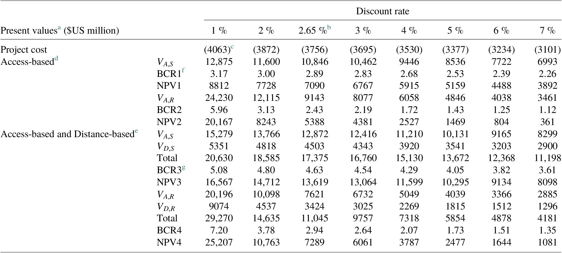
Abbreviations: BCR, benefit-cost ratio; NPV, net present value.
a All values have been discounted to year 2007 when Second Avenue Subway Phase 1 actually started to construct, and the unit of account is $US million.
b The discount rate of 2.65 % is designated by the Federal Transit Administration when preparing Environmental Impact Statement for Second Avenue Subway Phase 1.
c Values in parentheses are expenditures (outflows), and negatively contribute to Net Present Value.
d Under Access-based section, the calculation of total $ {V}_{A,S} $
uses coefficients in Model 1 in Table 7 and
$ {V}_{A,S} $
uses coefficients in Model 1 in Table 7 and $ {V}_{A,R} $
uses coefficients in Model 1 in Table 5.
$ {V}_{A,R} $
uses coefficients in Model 1 in Table 5.
e Under Access-based and Distance-based section, the calculation of total $ {V}_{A,S} $
and
$ {V}_{A,S} $
and $ {V}_{D,S} $
uses coefficients in Model 2 in Table 7 and
$ {V}_{D,S} $
uses coefficients in Model 2 in Table 7 and $ {V}_{A,R} $
and
$ {V}_{A,R} $
and $ {V}_{D,R} $
use coefficients in Model 3 in Table 5.
$ {V}_{D,R} $
use coefficients in Model 3 in Table 5.
f BCR1(2) is the BCR calculated by $ {V}_{A,S} $
(
$ {V}_{A,S} $
( $ {V}_{A,R} $
) divided by project cost, and NPV1(2) is the result of
$ {V}_{A,R} $
) divided by project cost, and NPV1(2) is the result of $ {V}_{A,S} $
(
$ {V}_{A,S} $
( $ {V}_{A,R} $
) minus project cost.
$ {V}_{A,R} $
) minus project cost.
g BCR3(4) is calculated by the sum of total $ {V}_{A,S} $
(
$ {V}_{A,S} $
( $ {V}_{A,R} $
) and total
$ {V}_{A,R} $
) and total $ {V}_{D,S} $
(
$ {V}_{D,S} $
( $ {V}_{D,R} $
) divided by project cost, and NPV3(4) is the result of the sum minus project cost.
$ {V}_{D,R} $
) divided by project cost, and NPV3(4) is the result of the sum minus project cost.
First, as shown by the Access-based section, if we only consider the impact of job accessibility, we find that the BCR based on sold properties’ value appreciation ranges between 2.26 and 3.17, and that the BCR based on rented properties’ lies between 1.12 and 5.19. When adding the influence of shortened distance to the nearest subway station (Access-based and Distance-based section), we observe that the BCR range for sold properties jumps to 3.61–5.08, and that that range for rental properties rises to 1.35–7.2. The range for BCR of rented properties is wider because the perpetuity discounting model is more sensitive to the variation of discount rate (since rents are in the future, whereas sold valuations are in the present, and already embed market expectations about discounted values). Second, property value appreciation triggered by reduced distance to the nearest subway station is far smaller than that caused by improved job accessibility, conveying that house price is more sensitive and responsive to variation in job accessibility.
In short, all the BCRs shown in Table 8 are greater than 1, and all the NPVs are positive, epitomizing that the value appreciation in residential properties in adjacent neighborhoods is large enough to cover the total project cost of Phase I of the Second Avenue Subway. We anticipate including commercial properties would increase BCR and NPV further.
Table 9 summarizes the BCA results for the Second Avenue Subway. First, the actual total capital cost for Phase I was about $US 4 billion, which is 77.15 % of the total (Phases I and II) estimated project cost $US 5.1 billion for Alternative 1. However, as specified in 1999 DEIS (The Metropolitan Transportation Authority, 1999), a total of $US 5.1 billion was planned for constructing five new subway stations and the 6 km long northern Second Avenue Subway line (from 64th Street to 129th street). It has already spent more than $US 4 billion to build the first phase of the Second Avenue Subway (63rd Street to 96th Street), which is about 3 km long and has three new subway stations (The Metropolitan Transportation Authority, 2017).
Table 9. Comparison of project cost effectiveness measures.

Note: We modified this table based on the original table sourced from the DEIS established by The Metropolitan Transportation Authority (1999).
Abbreviations: BCR, benefit-cost ratio; DEIS, Draft Environmental Impact Statement; TSM, transportation systems management.
a In line with the analysis method applied MTA in preparation for DEIS, the discount rate is 2.65 %.
b The base year applied when discounting project cost and benefits to present value is the year of construction begin, which is 2004 for alternatives in DEIS and 2007 for Actual(2018). In addition, a 50 year forecast horizon is taken when accumulate the present value for customer and social benefits.
c Raw project costs for DEIS alternatives are reported in 1997 $US, and the actual project was lastly updated in 2017. All project cost has been inflated to $US 2018 with Gross Domestic Product deflator established by the World Bank.
d This is the sum of AV and DV if all properties were sold, listed in Table 8.
e This is the sum of AV and DV if all properties were rented, listed in Table 8.
Furthermore, if we convert the total capital cost to unit cost, the actual unit cost of $US 1.4 billion per km is much higher than the estimated cost of $US 850 million per km in DEIS in real dollars. The actual unit cost is also higher than the unit cost of the proposed full-length Second Avenue Subway (13.7 km from 125th Street in East Harlem to Financial District in Lower Manhattan), which is approximately $US 1.2 billion per km (total cost is now predicted to be $US 16.8 billion; The Metropolitan Transportation Authority, 2004). The remainder of the originally proposed northern part of the Second Subway Avenue Line (99th Street to 125th Street), namely the second phase of the Second Avenue Subway line, will be delivered later than 2025 (The Metropolitan Transportation Authority, 2004, 2018). As a result, both the total capital cost and the unit cost of Phase 1 Second Avenue Subway exceed the expectations.
Then, among the three alternatives, the highest BCR is observed in the TSM option because of the lowest initial capital outflow, but both TSM and Alternative 2 were eliminated in preliminary engineering analysis. Alternative 1 was the locally preferred alternative which is comparable to the actual condition in 2018. The BCR of Alternative 1 is 1.31. As discussed in Section 5.1, if we only consider the $US 4.8 billion transit TTS benefit, the BCR of Alternative 1 is approximately equal to 0.95. However, the actual annual transit patronage and transit TTS per trip in 2018 are only 60 and 37.5 % of the expectations in Alternative 1, and the actual capital cost is higher than the predicted cost. The actual BCR of Phase 1 is lower than 1.
However, when we move to the residential properties’ value appreciation, both for sold properties and rental properties, the NPVs and BCRs outperform those for alternative project options listed in DEIS. The total capitalized value appreciation in sold properties is $US 17.37 billion, which is over four times larger than project cost. For rented properties, the value appreciation amounts to $US 11.04 billion, nearly three times the total project cost. In the project planning phase, these nonuser gains should have been reckoned with grounded on that this value increment stems from the Second Avenue Subway and is transferred to property owners as true economic wealth. In accordance with the decision rule of NPV and BCR, the results generated by property value appreciation approaches are in strong support of the decision on approving and constructing the Second Avenue Subway.
8 Implications on value capture
In the USA, historically prevailing funding sources earmarked for transport infrastructure construction are taxes levied on motor fuel, fees charged for the use of roadways and public transit services, and general purpose taxes like property taxes (Istrate & Levinson, Reference Istrate and Levinson2011; Zhao et al., Reference Zhao, Iacono, Lari and Levinson2012). They insist that the sustainability of those funding sources is nevertheless increasingly uncertain due to the advocacy of clean energy, the transformation of vehicle type, and the public resistance to tax rises. Value capture, an alternative mechanism to finance public infrastructure, uses the gains accrued to land or property value and ultimately received by private owners to recoup the costs incurred to construct the public infrastructure (Batt, Reference Batt2001; Mathur, Reference Mathur2014). In comparison to the traditional project financing scheme, value capture strategies remain sparsely applied in the USA. In addition, value capture is more commonly considered and adopted by transit projects rather than by road projects (Batt, Reference Batt2001). Findings from this paper may provide some insights.
First, as of the second year of operation of the Second Avenue Subway, the accumulated property value appreciation has exceeded the upfront capital cost, demonstrating the significant impact of transit infrastructure on property value and thus indicating the viability of value capture strategy. But be careful when drawing on this experience since New York is one of the most expensive city in the world, the continuation of land value appreciation here is doubtless relative to cities which are sparsely populated and less prosperous.
Second, unlike many traditional funding sources which are collected mainly grounded on the actual usage or operation status of the transport infrastructure, value capture strategies apply to the capitalized incremental accessibility generated by the new subway service. Given its independence from actual usage, cash inflows created under value capture are supposed to be foreseeable and sustainable.
Third, because different types of property transactions materialize value appreciation in distinct manners, customized value capture strategies on different transactions can be employed to ensure that different benefit inflows cover cost outflows of similar natures. Specifically, property purchase transactions initiated at early project planning stage and realize appreciation gains in larger size, which suit to accumulate benefit streams to recover upfront capital expenditure. Appreciation gains acquired through property lease emerge after project completion, in smaller size but at higher frequency, which might be able to cover periodic project operation and maintenance costs. Alternatively, a more general land value tax can be used, which will would eventually recover the gains in terms of property value appreciation.
9 Conclusion
In this paper, we hypothesize that unlike the traditional perspective of quantifying travel time and cost savings, the change in value of real estate better captures the economic impact of transport services more quickly, directly, and properly. In the case of the New York Second Avenue Subway project, first we find that both the observed transit ridership and the transit TTS per trip are lower than the forecast, so the actual transit person TTS benefit, which accounts for more than 70 % of total project economic benefit, is lower than originally estimated. Although the transit patronage is expected to rise after completing the second phase of the Second Avenue Subway, TTS for trips heading to South Manhattan may not be significantly improved until the operation of full-length Second Avenue Subway.
Second, a strong positive correlation between job accessibility by transit and housing price (both selling price and rental price) has been observed. According to the panel pooling model and hedonic model, if the total number of job opportunities that are accessible within 30 min by transit increases by 100,000, the rental price per square meter is expected to increase by 1.7–2.67 %, and the selling price per square meter is anticipated to rise by 2.72–3.23 %.
Third, the NPV of appreciation in residential property value due to the announcement of the Second Avenue Subway ranges from $US 3.8 billion to $US 8.8 billion, depending on the discount rate applied. The NPV of appreciation in residential rent due to the opening of the Second Avenue Subway range from $US 361 million to $US 20.2 billion, depending on the discount rate applied.
Furthermore, in Table 8, all BCRs are greater than 1, and all the NPVs are positive, implying that the appreciation in residential properties is large enough to cover the total project cost. In contrast, the BCR weighing TTS against total project is less than 1. As a result, in accordance with the decision rule of BCR and NPV, the value appreciation of residential properties brought by the Second Avenue Subway is greater than project cost, so constructing this subway is supported.
In summary, the access-based property value and rental value uplift assessment methods remedy many issues in the problematic traditional time-saving-based BCA evaluation method, and provide implication on using value capture strategy as an alternative project financing mechanism. Including and quantifying the economic impact of a new transport project on surrounding real estate may provide insightful information when evaluating and selecting transport projects. We also suggest this may be simpler to analyze than the traditional TTS approach as it does not require a full transport model, simply public transport schedules, and real estate data.
Author Contributions
Both authors contributed to the research conception and design. Data collection, analysis, and results interpretation were guided by Professor Levinson and performed by Y.W. Draft manuscript was prepared by Y.W., and D.L. edited and commented the draft manuscript. Both authors have read and agreed to submit the final manuscript.
Acknowledgement
The authors confirm that no funding was received for this research article.


 Open access