2.1. The current APG TBL database

The current database is a DNS database of a non-equilibrium APG TBL with a Reynolds number based on momentum thickness ($Re_\theta$) reaching up to $8000$. The code used to perform the DNS solves the three-dimensional incompressible Navier–Stokes equations. It provides the time evolution of three-dimensional velocity and pressure fields for a given flow configuration. The DNS code employs a hybrid MPI/OpenMP approach for parallelization. Further details on the code can be found in Simens et al. (Reference Simens, Jiménez, Hoyas and Mizuno2009) and Borrell, Sillero & Jiménez (Reference Borrell, Sillero and Jiménez2013).

The DNS computational set-up consists of two simulation domains, the auxiliary and main domains, running concurrently as described in Sillero, Jiménez & Moser (Reference Sillero, Jiménez and Moser2013) and Gungor et al. (Reference Gungor, Maciel, Simens and Soria2016). The auxiliary ZPG TBL DNS, with a coarser resolution, are intended to provide the realistic turbulent inflow data for the main APG TBL DNS. The goal of using two domains is to provide inflow conditions for the main DNS with lower computational cost. Regarding the other boundary conditions, the bottom surface is a flat plate with a no-slip boundary condition. The side boundary conditions are periodic. The far-field boundary condition is adjusted in the form of suction and blowing to apply adverse/favourable pressure gradients. The outflow condition is a Neumann boundary condition. The computational domain of the main APG TBL simulation, a rectangular volume with streamwise, wall-normal and spanwise lengths $(L_x, L_y, L_z)/\delta _{av} = (25.3,4.8,7.1)$, is discretized with $N_x\times N_y\times N_z =4609\times 736\times 1920$ grid points. Here, the average boundary layer thickness ($\delta _{av}$) is calculated within the useful range (or so-called domain of interest), which is the zone between the vertical dashed lines in figure 1.

Figure 1. Streamwise development of the main parameters of the APG TBL. (a) The suction/blowing boundary condition $V_{top}$ and edge velocity $U_e$. (b) Pressure gradient parameters $\beta _{ZS}$ and $\beta _{RC}$. (c) Shape factor $H$ and skin friction coefficient $C_f$. (d) Parameters $\delta$, $\delta ^*$ and $\theta$ normalized with their values at inlet. (e) Reynolds numbers $Re_\theta$ and $Re_\tau$. The vertical dashed lines are the boundaries of useful range. The open circles denote the three streamwise positions that are used in the paper.

Figure 1 shows the spatial development of main parameters of the APG TBL. As stated before, the pressure gradient in the APG TBL is generated by imposing a suction/blowing boundary condition for the wall-normal component of the velocity at the top boundary ($V_{top}$). Figure 1(a) shows the spatial development of $V_{top}$ along with the edge velocity $U_e$. The definition of $U_e$ is not straightforward in flows with inviscid velocity that varies in the wall-normal direction, such as the current flow. Although it is not the most generally applicable definition (see, for instance, Griffin, Fu & Moin Reference Griffin, Fu and Moin2021), we utilize the maximum streamwise component of the mean velocity in the wall-normal direction as $U_e$ for this study, to be consistent with most of the literature (Gungor et al. Reference Gungor, Maciel, Simens and Soria2016; Maciel et al. Reference Maciel, Wei, Gungor and Simens2018) and because it works for the flow cases studied here.

At the beginning of the domain, the suction velocity increases sharply within a short distance to impose the desired pressure gradient distribution. Downstream of this region, the suction velocity is adjusted to obtain a regularly increasing shape factor $H$ (figure 1c). The change in $V_{top}$ near the end of the computational domain is to increase the numerical stability of the simulation by accelerating the flow so that the Neumann boundary condition still holds. The suction boundary condition decelerates the flow, which is seen from the development of the edge velocity $U_e$ in figure 1(a).

Figure 1(b) shows two pressure gradient parameters that characterize the effect of the pressure gradient on the outer layer: $\beta _{RC}$, the Rotta–Clauser pressure gradient parameter, and $\beta _{ZS}$, the pressure gradient parameter based on the Zagarola–Smits velocity, defined as

(2.1a,b)\begin{equation} \beta_{RC}= \frac{\delta^*}{\rho u_\tau^2}\,\frac{{\rm d}P_e}{{\rm d}\,x}, \quad \beta_{ZS}= \frac{\delta}{\rho U_{ZS}^2}\,\frac{{\rm d}P_e}{{\rm d}\,x}. \end{equation}

Here, $\delta ^*$ is the displacement thickness, $\rho$ is the density, $u_\tau$ is the friction velocity, $P_e$ is the pressure at the edge of the boundary layer, and $U_{ZS}$ is the Zagarola–Smits velocity (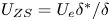$U_{ZS}=U_e\delta ^*/\delta$) (Zagarola & Smits Reference Zagarola and Smits1998). The traditionally used pressure gradient parameter, $\beta _{RC}$, increases progressively until $\beta _{RC}$ is above $350$, and then sharply decreases. However, as Maciel et al. (Reference Maciel, Wei, Gungor and Simens2018) demonstrated, it is not a valid pressure gradient parameter for TBLs with large velocity defect. Parameter $\beta _{ZS}$, which represents the local impact of the pressure gradient on the boundary layer regardless of velocity defect (Maciel et al. Reference Maciel, Wei, Gungor and Simens2018), increases near the flow entrance up to 0.35, and then decreases to approximately 0.05 and remains mostly the same in the last part of the domain. The rapid increase of $\beta _{ZS}$ at the beginning of the domain causes the increase in momentum loss in the boundary layer ($H$ increases; figure 1c). The subsequent decrease of $\beta _{ZS}$ over most of the domain should lead theoretically to momentum gain in the boundary layer ($H$ decreases). However, because the boundary layer responds with a delay to the pressure force evolution, the momentum gain occurs only at the end of the domain.

The effect of the pressure gradient on the flow is also seen in the development of the skin friction coefficient $C_f$, as shown in figure 1(c); $C_f$ decreases steadily until around $x/\delta _{av}\approx 20$, and becomes very close to zero. The behaviour of $C_f$ and $H$ reflects the strong non-equilibrium nature of the current APG TBL flow.

Figure 1(d) shows the spatial development of $\delta$, $\delta ^*$ and momentum ($\theta$) thicknesses. They all increase until close to the end of the domain. Figure 1(e) shows the distributions of the most commonly used Reynolds numbers for TBLs, $Re_\theta$ and $Re_\tau$; $Re_\theta$ increases approximately from 2000 to 8000. The Reynolds number based on $u_\tau$, $Re_\tau$, develops irregularly in the streamwise direction. However, it is not valid because $u_\tau$ is not a valid scale for APG TBLs with large velocity defect. The irregularity of $Re_\tau$ stems from utilizing $u_\tau$ as a velocity scale.

2.2. Existing databases

Because we focus on spectral analysis in the current paper, we have two criteria for selecting existing databases of ZPG TBLs and channel flows: sufficiently high Reynolds number and availability of spectral distributions of Reynolds stresses, production and pressure-strain. The DNS database of Lee & Moser (Reference Lee and Moser2015) with $Re_\tau =2000$ is employed for channel flows. This database is chosen because some one-dimensional (1-D) and two-dimensional (2-D) spectra are available as functions of streamwise and spanwise wavenumbers ($k_x$, $k_z$) and $y$. The DNS database of Sillero et al. (Reference Sillero, Jiménez and Moser2013) with $Re_\theta =6500$ and the experimental database of Baidya et al. (Reference Baidya, Philip, Hutchins, Monty and Marusic2021) with $Re_\theta =6191$ are chosen for ZPG TBLs. We chose these two databases for ZPG TBLs because the Reynolds numbers are similar and the 1-D spectral distributions of Reynolds stress and production are available as functions of $k_z$ and $y$ for the database of Sillero et al. (Reference Sillero, Jiménez and Moser2013), and $k_x$ and $y$ for the database of Baidya et al. (Reference Baidya, Philip, Hutchins, Monty and Marusic2021). They complement each other for the spectral analysis without introducing any significant Reynolds number effect.

2.3. Flow description

We aim to investigate a wide range of velocity defect cases in this study. Three streamwise positions from the APG TBL are employed. These streamwise positions, as shown in figure 1, represent three velocity defect cases, and their corresponding shape factors are $1.65$, $2.00$ and $2.63$. The shape factor is $1.35$ for both ZPG TBL cases since they are at similar Reynolds numbers. The velocity defect is smaller in the ZPG TBL than the small-defect case of the APG TBL. As for the channel flow, the velocity defect, which is with respect to the centreline velocity, is smaller than values for the ZPG TBLs as it is well-known. These five flow cases, details of which are provided in table 1, cover a wide range of velocity defect situations, from a channel flow to a TBL with a large velocity defect.

Table 1. Information about the databases used in the paper: ZPGa, ZPGb, and CH indicate the databases of Sillero et al. (Reference Sillero, Jiménez and Moser2013), Baidya et al. (Reference Baidya, Philip, Hutchins, Monty and Marusic2021) and Lee & Moser (Reference Lee and Moser2019), respectively.

Regarding the Reynolds numbers of the cases, the ZPG TBL and the channel flow cases have similar $Re_\tau$ and are selected at higher $Re_\tau$ and $Re_\theta$ than the APG TBL cases. We could have chosen different databases for ZPG TBLs, or channel flows with a lower Reynolds number, instead. However, it is better to analyse canonical flows at high Reynolds number because of the elevated outer-layer activity in such flows (Hutchins & Marusic Reference Hutchins and Marusic2007a). In this manner, we can compare the outer peaks of the spectral distributions of canonical flows and APG TBLs.

Throughout the paper, the streamwise, wall-normal and spanwise directions are referred to as $x$, $y$ and $z$, or $1$, $2$ and $3$ for index notation. The corresponding instantaneous velocity components are $\bar {u}$, $\bar {v}$ and $\bar {w}$. The brackets $\langle \cdot \rangle$ denote ensemble averaging. Furthermore, uppercase and lowercase letters denote the mean value and the fluctuations, respectively. Thus $\langle \bar {u}_i\rangle =U_i$ and $\bar {u}_i=U_i+u_i$. The upper index $+$ means the friction-viscous scales, with the friction velocity $u_\tau$ as the velocity scale, and $\nu /u_\tau$ as the length scale.

3.1. Mean flow

Figures 2(a,b) present the outer- and inner-scaled mean velocities as functions of $y$ for all the databases. The outer-scaled mean velocity profiles demonstrate the momentum deficit in the APG TBL cases. As the flow develops under the effect of the APG, the defect in the mean velocity profile increases. The profile starts to resemble velocity profiles of mixing layers (Gungor et al. Reference Gungor, Maciel, Simens and Soria2016) in the large-defect case, with an inflection point in the middle of the boundary layer. The inner-scaled mean velocity profiles show that the mean velocity deviates from the log law in the APG TBL cases. Moreover, this deviation increases with increasing velocity defect. Furthermore, friction-viscous scales progressively fail to scale the mean velocity in the inner region as the defect increases (Gungor et al. Reference Gungor, Maciel, Simens and Soria2016; Maciel et al. Reference Maciel, Wei, Gungor and Simens2018).

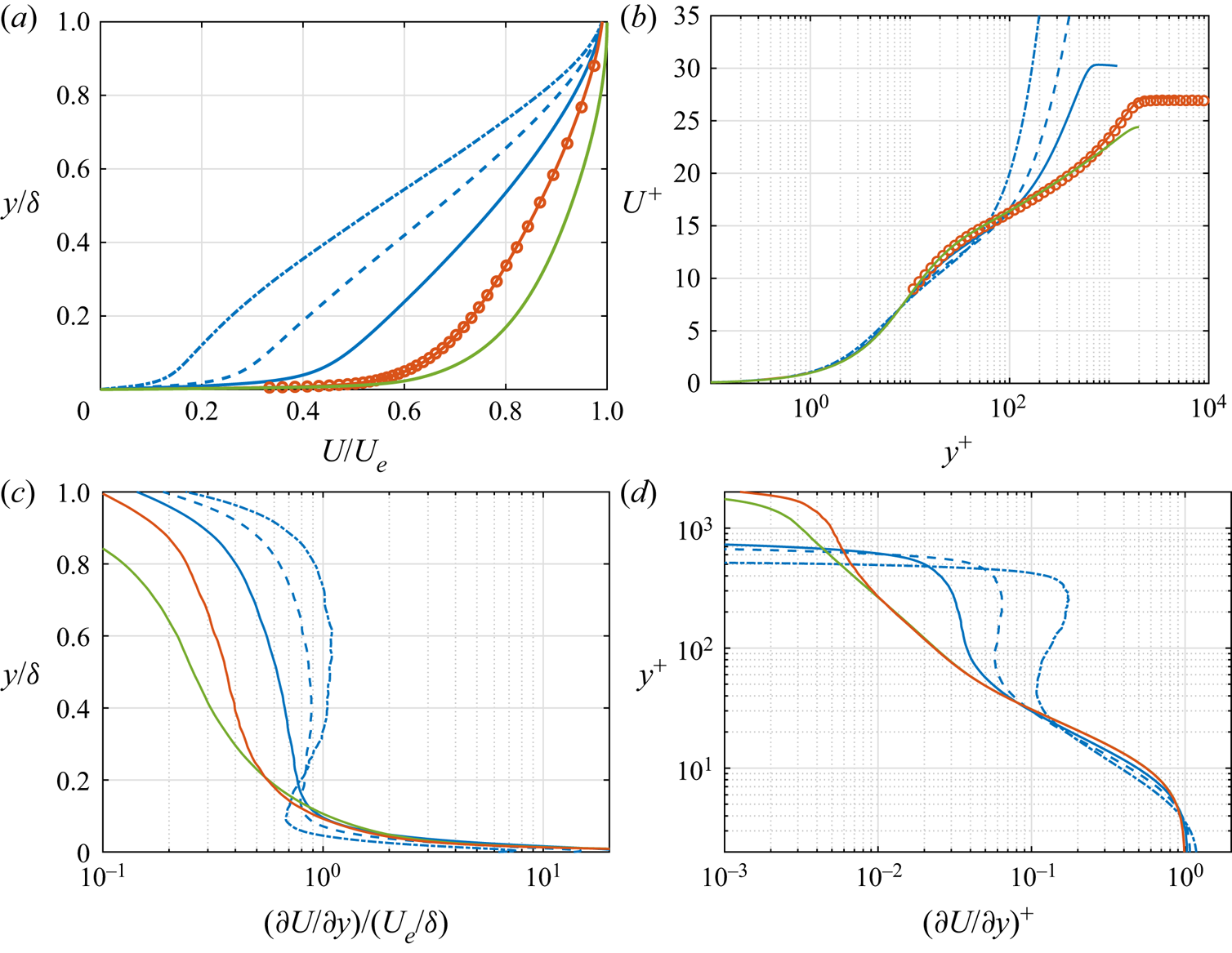
Figure 2. The mean velocity profiles of all databases normalized with (a) outer scales and (b) friction-viscous units, plus the mean shear profiles of the DNS databases normalized with (c) outer scales and (d) friction-viscous units. Legend as in table 1.

Figures 2(c,d) show the mean shear profiles for the DNS databases. The mean shear profile for the experimental ZPG TBL case is not given here due to lack of points near the wall. The mean shear distribution is important because it plays a role directly in turbulence production and hence turbulence in the flow. The change in the mean velocity profiles significantly affects the mean shear distribution in the outer layer. As the defect increases, the mean shear increases in the outer layer. More importantly, the relative magnitude of mean shear in the outer layer with respect to the inner layer increases with increasing velocity defect, as can be seen in figure 2(d). Regarding the inner layer, the mean shear remains fairly similar when it is normalized with friction-viscous scales, as expected, despite the direct effect of the pressure force near the wall in the APG TBL cases. The impact of the varying mean shear on turbulence will be discussed further in § 5.

3.2. Reynolds stresses

Figure 3 presents the wall-normal distribution of the components of the Reynolds stress tensor for all cases. The inner scales scale the Reynolds stresses well for the canonical flows. The $\langle u^2 \rangle$ profiles of the channel flow and ZPGa collapse perfectly with friction-viscous units, as expected. The $\langle u^2 \rangle$ levels are slightly smaller in ZPGb than in ZPGa in the inner layer, but this is due to the lack of spatial resolution of the probe used in the experiments (Baidya et al. Reference Baidya, Philip, Hutchins, Monty and Marusic2017).

Figure 3. Reynolds stress profiles normalized with (a) friction-viscous units and (b) outer scales. Legend as in table 1.

The change in the mean shear in the APG TBL (figures 2c,d) changes the Reynolds stress profiles progressively. The $\langle u^2 \rangle$ profiles are still fairly similar for APG1 and canonical wall-bounded flows in the inner layer, even if the scaled amplitude increases. The inner peak for $\langle u^2\rangle$ still exists in APG1. However, such a similarity is not encountered for the other components of the Reynolds stress tensor. Moreover, figure 3(b) shows that the turbulent activity in the inner layer diminishes with respect to that in the outer layer as the defect increases. The outer layer becomes dominant as the mean shear increases in the outer layer. In the large-defect cases, APG2 and APG3, all components peak in the middle of the boundary layer, where the mean shear has a plateau. Regarding the magnitude of the Reynolds stresses, the levels increase progressively with increasing velocity defect when Reynolds stresses are normalized with friction-viscous scales because they are not appropriate scales for large velocity defect cases (Maciel et al. Reference Maciel, Wei, Gungor and Simens2018). It is important to state that $U_e$ is not necessarily an appropriate outer scale either (Maciel, Rossignol & Lemay Reference Maciel, Rossignol and Lemay2006a); however, it conserves the order of magnitude of Reynolds stresses in the range of velocity defects and Reynolds numbers of the cases examined here.

The Reynolds stress profiles of the current APG TBL case are consistent with APG TBL cases in the literature. In the small-defect case, there is an inner peak for $\langle u^2 \rangle$ and an elevated outer layer activity for all Reynolds stress components. This has been reported for equilibrium (Skåre & Krogstad Reference Skåre and Krogstad1994; Lee Reference Lee2017) and non-equilibrium (Gungor et al. Reference Gungor, Maciel, Simens and Soria2016) cases in small-defect APG TBLs. Moreover, the $y$-position and energy levels of the inner peak match well when the velocity defects of the cases are similar (Kitsios et al. Reference Kitsios, Atkinson, Sillero, Borrell, Gungor, Jimënez and Soria2016; Tanarro et al. Reference Tanarro, Vinuesa and Schlatter2020). Regarding the large-defect case, other researchers have already reported the increasing importance of the outer layer as the mean shear increases in the outer layer (Skåre & Krogstad Reference Skåre and Krogstad1994; Gungor et al. Reference Gungor, Maciel, Simens and Soria2016; Kitsios et al. Reference Kitsios, Sekimoto, Atkinson, Sillero, Borrell, Gungor, Jimënez and Soria2017).

3.3. Reynolds stress budgets

To understand the energy transfer mechanisms in APG TBLs, the budget of the Reynolds stress tensor is investigated first through the transport equations for the Reynolds stresses:

(3.1)\begin{align} 0&={-} \left(\langle u_i u_k\rangle\,\frac{\partial U_j}{\partial x_k}+ \langle u_j u_k\rangle\,\frac{\partial U_i }{\partial x_k} \right ) - \frac{\partial \langle u_iu_ju_k\rangle}{\partial x_k} \nonumber\\ &\quad + \left\langle \frac{p}{\rho} \left(\frac{\partial u_i}{\partial x_j}+\frac{\partial u_j}{\partial x_i}\right) \right \rangle - \frac{1}{\rho}\,\frac{\partial}{\partial x_k} (\langle u_i p\rangle \delta_{jk}+\langle u_j p\rangle \delta_{ik})\nonumber\\ &\quad - 2\nu \left\langle \frac{\partial u_i}{\partial x_k}\,\frac{\partial u_j}{\partial x_k}\right\rangle+ \nu\,\nabla^2 \langle u_iu_j\rangle - U_k\,\frac{\partial \langle u_i u_j \rangle }{ \partial x_k}. \end{align}

Here, $\nu$ is viscosity and $\delta _{ik}$ is the Kronecker delta function. In order, the terms are production, turbulent transport, pressure-strain, pressure transport, viscous dissipation, viscous transport and mean convection.

Figure 4 presents Reynolds stress budgets for canonical flows, and small- and large-defect APG TBLs. The profiles are plotted with logarithmic and linear axes to emphasize inner and outer layer, as mentioned before. The Reynolds stress budget distributions show that energy follows the same main path in both inner and outer layers, regardless of the flow, as expected. Energy is extracted from the mean flow through $\langle u^2 \rangle$ production. Some of this energy is transferred to $\langle v^2 \rangle$ and $\langle w^2 \rangle$ through pressure-strain, which is a sink term for $\langle u^2 \rangle$ and a source term for the other normal components except in the very near-wall region. Energy is also transported or dissipated in all components. Furthermore, $\langle v^2 \rangle$ production, which is zero for channel flows and negligible for ZPG TBLs, is a sink term that transfers energy back to the mean flow in the outer region for APG TBLs. Regarding the Reynolds shear stress, the production and pressure-strain are almost in balance in all cases except in the near-wall region.

Figure 4. The Reynolds stress budgets. The levels and axes are normalized with (a) the friction-viscous scales and (b) outer scales. The rows are for $\langle u^2\rangle$, $\langle v^2\rangle$, $\langle w^2\rangle$ and $\langle uv\rangle$ for each panel. Production, dark blue solid line; dissipation, red solid line; pressure-strain, yellow solid line; viscous diffusion, green solid line; turbulent transport, purple solid line; mean convection, brown solid line; pressure transport, blue solid line.

The magnitudes of the budget terms are very similar for CH and ZPGa for the inner-scaled profiles. However, the levels increase drastically as the defect increases when normalized with $u_\tau$, consistently with the trend that we observe in the Reynolds stress profiles, which again confirms that $u_\tau$ is not a proper inner scale for APG TBLs with large velocity defect.

In the inner region, as figure 4(a) shows, the behaviours of the Reynolds stress budgets of the canonical flows and APG1 are almost the same for all normal components, regardless of the velocity defect. The shapes of the budget profiles are almost identical, with a minor shift in $y^+$. For instance, the $\langle u^2 \rangle$ production peak is at $y^+\approx 11$ and $9$ in canonical flows and APG1, respectively. A clear difference between canonical flows and APG1 is that the turbulent and pressure transport above $y^+\approx 10$ for $\langle v^2 \rangle$ are negligible for APG1.

As the mean shear distribution changes from APG1 to APG3, the overall behaviour of the source and sink terms (production, pressure-strain and dissipation) in the inner layer does not change considerably except for the aforementioned difference in magnitude. Besides the magnitude change, the main difference is that they start to increase with $y$ above $y^+=30$ because they all peak in the outer layer, as is discussed later. The change of relative importance between the inner and outer layers affects turbulent transport, as well. It becomes a gain term for $\langle u^2 \rangle$ and $\langle v^2 \rangle$ in most of the inner layer due to the elevated turbulent activity in the outer layer of the large-defect case. This behaviour is also reported in equilibrium APG TBL cases for $\langle u^2 \rangle$ (Kitsios et al. Reference Kitsios, Sekimoto, Atkinson, Sillero, Borrell, Gungor, Jimënez and Soria2017).

The Reynolds stress fluxes due to turbulent transport in the wall-normal direction, where the flux is $\theta _{ii} = \langle u_iu_iu_2\rangle$, are given for ZPGa, APG1 and APG3 in Appendix A (figure 17). The $\langle u^2 \rangle$ flux towards the wall is below $y^+=11$ in ZPGa and APG1. In contrast, fluxes towards the wall start as high as $y/\delta =0.4$ ($y^+\approx 200$) in APG3, and for all Reynolds normal stresses. Strong turbulent transport towards the wall in the lower half of a near-equilibrium large-defect APG TBL was also reported by Skåre & Krogstad (Reference Skåre and Krogstad1994).

Regarding the outer layer, as shown in the outer-scaled profiles in figure 4(b), production, pressure-strain and dissipation are at high levels between $y/\delta =0.1$ and $0.3$ in APG1, much like the Reynolds stresses themselves, but no peak is present in the outer layer. Despite the lack of an outer peak in APG1, a plateau between approximately $y/\delta =0.1$ and $y/\delta =0.3$ that is not observed in the channel flow and the ZPG TBL exists in production and pressure-strain terms. In the large-defect case, an outer peak emerges for the source and sink terms at around $y/\delta =0.5$. Such a behaviour has been reported before for equilibrium (Skåre & Krogstad Reference Skåre and Krogstad1994; Kitsios et al. Reference Kitsios, Sekimoto, Atkinson, Sillero, Borrell, Gungor, Jimënez and Soria2017) and non-equilibrium APG TBLs (Gungor et al. Reference Gungor, Maciel, Simens and Soria2016).

4.1. Methodology

We will first present the transport equation for the two-point correlation tensor. Let $x_i$ and $\tilde {x}_i$ be the components of the coordinates of the two points used to compute the correlations, defined as

(4.1)\begin{equation} \tilde{x}_i=x_i+r_i, \end{equation}

where $r_i$ is the separation length between these points in direction $i$. Further, let the velocity components at ${x_i}$ and $\tilde {x}_j$ be $u_i$ and $\tilde {u}_j$. Starting from the Navier–Stokes equations, the transport equations of the two-point correlation tensor $\textsf{{R}}_{ij}=\langle u_i \tilde {u}_j \rangle$ can be obtained in the form

(4.2) \begin{align} \left\langle \tilde{u}_j\,\frac{\partial u_i}{\partial t} + u_i\,\frac{\partial \tilde{u}_j}{\partial t} \right \rangle &={-} \underbrace{\left[ U_k \left \langle \tilde{u}_j\,\frac{\partial u_i}{\partial x_k} \right \rangle + \tilde{U}_k \left\langle u_i\,\frac{\partial \tilde{u}_j}{\partial \tilde{x}_k} \right\rangle \right]}_{{\mathsf{R}}_{ij}^A} - \underbrace{ \left[\langle \tilde{u}_j u_k \rangle\,\frac{\partial U_i}{\partial x_k} + \langle u_i \tilde{u}_k \rangle\,\frac{\partial \tilde{U}_j}{\partial \tilde{x}_k} \right]}_{{\mathsf{R}}_{ij}^P}\nonumber\\ &\quad - \underbrace{ \left [ \left\langle \tilde{u}_j\,\frac{\partial u_k u_i}{\partial x_k} \right \rangle + \left \langle u_i\,\frac{\partial \tilde{u}_k \tilde{u}_j}{\partial \tilde{x}_k} \right \rangle \right]}_{{\mathsf{R}}_{ij}^T} - \underbrace{ \frac{1}{\rho}\left [ \left\langle \tilde{u}_j\, \frac{\partial p}{\partial x_i} \right \rangle + \left\langle u_i\,\frac{\partial \tilde{p}}{\partial\tilde{x}_j} \right\rangle \right]}_{{\mathsf{R}}_{ij}^{\varPi}}\nonumber\\ &\quad + \underbrace{ \left [ \nu \left\langle \tilde{u}_j\,\frac{\partial^2 u_i}{\partial x_k\,\partial x_k} \right \rangle + \nu \left \langle u_i\,\frac{\partial^2 \tilde{u}_j}{\partial \tilde{x}_k\, \partial \tilde{x}_k} \right \rangle \right]}_{{\mathsf{R}}_{ij}^\nu}. \end{align}

The terms on the right-hand side of the equation that are labelled as ${\mathsf{R}}_{ij}^A$, ${\mathsf{R}}_{ij}^P$, ${\mathsf{R}}_{ij}^T$, ${\mathsf{R}}^\varPi _{ij}$ and ${\mathsf{R}}^\nu _{ij}$, are advection, production, turbulent transport, pressure and viscous terms, respectively.

The transport equations need to be simplified to perform the spectral decompositions of the various terms. In this work, the correlations are computed only in the streamwise and spanwise directions. Therefore, there is no separation in the wall-normal direction (see (4.3a)). Since all the flows considered here are homogeneous in the spanwise direction, the derivative of the mean velocity with respect to $x_3$ and the mean velocity in $x_3$ are zero (see (4.3b)). Finally, $u_i$ is independent of $\tilde {x}_{\alpha }$ since $u_i$ is the velocity component at another location, and this is valid for $\tilde {u}_i$ and $x_\alpha$, too. Thus their corresponding derivatives are zero (see (4.3c)). We have

(4.3a)$$\begin{gather} \tilde{x}_2 =x_2, \end{gather}$$

(4.3b)$$\begin{gather}\frac{\partial U_i}{\partial x_{3}} = U_3 = 0, \end{gather}$$

(4.3c)$$\begin{gather}\frac{\partial u_i}{\partial \tilde{x}_{\alpha}} = \frac{\partial \tilde{u}_j}{\partial x_{\alpha}} = 0, \quad \alpha=1,2,3. \end{gather}$$

We need to write (4.2) as a function of separation lengths, $r_1$ and $r_3$, to obtain the spectral distributions. Therefore, we need to substitute the independent variables $x_i$ and $\tilde {x}_i$. As is usually done, the second substitution variable (associated with $r_i$) is chosen as the average position of the two points:

(4.4)\begin{equation} \varGamma_\alpha = (\tilde{x}_\alpha+x_\alpha)/2, \quad \alpha=1,3. \end{equation}

Let $\varPhi$ be any type of two-point correlation in (4.2). We have the relationships

(4.5a)$$\begin{gather} \frac{\partial \varPhi}{\partial \varGamma_3} = 0, \end{gather}$$

(4.5b)$$\begin{gather}\frac{\partial \varPhi}{\partial \varGamma_1} \approx 0, \end{gather}$$

because the term $\partial \varPhi /\partial \varGamma _3$ is zero due to spanwise homogeneity (see (4.5a)), and the two-point correlations are assumed to vary slowly in the streamwise direction in the case of the TBLs (see (4.5b)). The latter assumption is strong in the case of the non-equilibrium APG TBL, but it is necessary to perform the spectral decompositions. Then we perform the transformation for two-point correlations as shown in (4.6). Note that the transformation does not apply to the derivatives of mean velocity in (4.2) since these derivatives are assumed constant in $x_1$ and $x_3$:

(4.6a)$$\begin{gather} \frac{\partial \varPhi_{}}{\partial x_\alpha} = \frac{\partial \varPhi_{}}{\partial \varGamma_\alpha}\,\frac{\partial \varGamma_\alpha}{\partial x_\alpha} + \frac{\partial \varPhi_{}}{\partial r_\alpha}\,\frac{\partial r_\alpha}{\partial x_\alpha} ={-} \frac{\partial \varPhi_{}}{\partial r_\alpha}, \end{gather}$$

(4.6b)$$\begin{gather}\frac{\partial \varPhi_{}}{\partial \tilde{x}_\alpha} = \frac{\partial \varPhi_{}}{\partial \varGamma_\alpha}\,\frac{\partial \varGamma_\alpha}{\partial \tilde{x}_\alpha} + \frac{\partial \varPhi_{}}{\partial r_\alpha}\,\frac{\partial r_\alpha}{\partial \tilde{x}_\alpha} = \frac{\partial \varPhi_{}}{\partial r_\alpha}. \end{gather}$$

Since we are interested in production and pressure-strain, we will discuss only these two terms hereafter. The production term in (4.2) can be rewritten by taking advantage of (4.3a) and (4.3b):

(4.7)\begin{equation} {\mathsf{R}}_{ij}^{P} ={-} \langle \tilde{u}_j u_1 \rangle\,\frac{\partial U_i}{\partial x_1} - \langle u_i \tilde{u}_1 \rangle\,\frac{\partial \tilde{U}_j}{\partial \tilde{x}_1} - \langle \tilde{u}_j u_2 \rangle\,\frac{\partial U_i}{\partial x_2} - \langle u_i \tilde{u}_2 \rangle\,\frac{\partial \tilde{U}_j}{\partial \tilde{x}_2}. \end{equation}

Furthermore, by assuming that the derivatives of the mean velocity with respect to $x_1$ and $x_2$ do not change in $x_1$, i.e.

(4.8)\begin{equation} \left.\begin{aligned} \frac{\partial \tilde{U}_k}{\partial \tilde{x}_1} & = \frac{\partial {U}_k}{\partial x_1}, \\ \frac{\partial \tilde{U}_k}{\partial \tilde{x}_2} & = \frac{\partial {U}_k}{\partial x_2}, \end{aligned}\right\}, \end{equation}

the production term can be rewritten as

(4.9)\begin{equation} {\mathsf{R}}_{ij}^{P} ={-} \langle \tilde{u}_j u_1 \rangle\,\frac{\partial U_i}{\partial x_1} - \langle u_i \tilde{u}_1 \rangle\,\frac{\partial {U}_j}{\partial {x}_1} - \langle \tilde{u}_j u_2 \rangle\,\frac{\partial U_i}{\partial x_2} - \langle u_i \tilde{u}_2 \rangle\,\frac{\partial {U}_j}{\partial {x}_2} . \end{equation}

In addition, the derivative of the mean velocity in the streamwise direction is zero for channel flows due to the streamwise homogeneity, and is negligible in the ZPG TBLs. Therefore, the production term is simplified for the canonical flow cases as

(4.10)\begin{equation} {\mathsf{R}}_{ij}^{P} ={-} \langle \tilde{u}_j u_2 \rangle\,\frac{\partial U_i}{\partial x_2} - \langle u_i \tilde{u}_2 \rangle\,\frac{\partial {U}_j}{\partial {x}_2} . \end{equation}

The pressure term in (4.2) is divided into two terms,

(4.11)\begin{equation} {\mathsf{R}}^\varPi_{ij} = {\mathsf{R}}_{ij}^d + {\mathsf{R}}_{ij}^s, \end{equation}

where ${\mathsf{R}}_{ij}^d$ and ${\mathsf{R}}_{ij}^s$ are pressure transport and pressure-strain, respectively. By taking advantage of the relationships and mathematical manipulations introduced previously, the pressure-strain term is written for the wall-parallel, $R_{\alpha \alpha }^s$, and wall-normal, $R_{22}^s$, directions as

(4.12)$$\begin{gather} R^s_{\alpha\alpha} = \frac{1}{\rho} \left\langle - {p}\,\frac{\partial {u}_i}{\partial r_\alpha } + \tilde{p}\,\frac{\partial \tilde{u}_j}{\partial r_\alpha} \right\rangle, \quad \alpha=1,3, \end{gather}$$

(4.13)$$\begin{gather}R^s_{22} = \frac{1}{\rho} \left ( \left \langle \tilde{p}\,\frac{\partial {u}_i}{\partial x_2 } \right \rangle +\left\langle {p}\,\frac{\partial \tilde{u}_j}{\partial \tilde{x}_2} \right \rangle \right). \end{gather}$$

There are several ways to perform the decomposition of the pressure term, but we chose this one for two reasons. First, we want to be consistent within the paper, because the spectral distributions of the channel flow that we use in the paper are obtained using the same decomposition as in Lee & Moser (Reference Lee and Moser2019). The other reason is that this decomposition is consistent with many studies in the literature (Mansour, Kim & Moin Reference Mansour, Kim and Moin1988; Mizuno Reference Mizuno2016) and, more importantly, with the Reynolds stress transport equation as written in (3.1) when $r_x$ and $r_z$ tend to zero. In other words, by integrating the spectral distributions of these terms over the wavenumbers, the budget of the Reynolds stresses, which is discussed in the previous section, is obtained.

The spectral distributions of production and pressure-strain are obtained by performing the Fourier transform of each term with respect to $r_x$ and $r_z$. In the paper, 1-D spectra are computed as functions of wavenumber component $k_x$ or $k_z$, and 2-D spectra as functions of $k_x$ and $k_z$. The derivation above is for the 2-D spectra, but a similar derivation is performed, albeit not given here, for the 1-D spectra.

We utilize temporal data to obtain the spectra in $k_x$. We invoke Taylor's frozen turbulence hypothesis to convert frequency into streamwise wavenumber

(4.14)\begin{equation} k_x = \frac{ 2 {\rm \pi}f}{ U_c}, \end{equation}

where $f$ is the sampling frequency, and $U_c$ is the convection velocity, which is taken to be the local mean velocity.

In the paper, the spectra are always plotted as pre-multiplied by the wavenumbers, and the wavenumber axes are always in logarithmic scale. For 1-D spectra, the wall-normal axis is plotted in linear scale for the outer layer and logarithmic scale for the inner layer, so that both layers are examined in a more detailed, clear way.

The premultiplied 1-D spectral distributions of energy (shaded), production (red) and pressure-strain (purple) as functions of $y$ and wavelength components $\lambda _x$ and $\lambda _z$ for all components of the Reynolds stress tensor are presented using friction-viscous scales in figure 5. In addition, the outer-scaled spectral distributions are given in figure 18 in Appendix B. The 1-D pressure-strain spectra are available only for the APG TBL cases. Furthermore, $\langle v^2 \rangle$ production is plotted only for the APG TBL cases due to the fact that it is zero for channel flows and negligible for ZPG TBLs.

Figure 5. The premultiplied 1-D energy (shaded contours), production (red contours) and pressure-strain (purple contours) spectra of the channel flow (first column), the ZPG TBLs (second column), APG1 (third column), and APG3 (fourth column) as functions of (a) $\lambda _z^+$ and (b) $\lambda _x^+$, and $y^+$. The rows in each panel are respectively $\langle u^2\rangle$, $\langle v^2\rangle$, $\langle w^2\rangle$ and $\langle uv\rangle$. The contour levels are $[0.1\ 0.3\ 0.5\ 0.7\ 0.9]$ of the maxima of spectra for energy, and $[0.3\ 0.7]$ of the maxima of spectra for production and pressure-strain. The dashed contours indicate negative values. The horizontal and vertical dashed lines indicate $y^+=10,100$ and $\lambda ^+=100,1000$.

4.2. Energy

We start by discussing the energy spectra (shaded contours) of the channel flow and ZPG TBLs. The spectral distribution of energy shows that energy-carrying structures are found mainly in the inner layer in the channel flow and ZPG TBLs, with some activity in the outer layer. A strong peak is located at $\lambda _z^+\approx 120$ and $\lambda _x^+\approx 1000$ in the inner layer for the $\langle u^2 \rangle$ spectra. It is associated with the well-known streamwise streaks in the near-wall region of canonical wall-bounded flows. As for the outer layer, the $\langle u^2 \rangle$ and $\langle uv \rangle$ distributions show an outer peak in the spanwise spectra. The streamwise spectra of CH and ZPGb do not exhibit a clear outer peak because $Re_\tau$ is not high enough. Channel flows and ZPG TBLs with higher $Re_\tau$ have a distinct outer peak in their streamwise spectra (Hutchins & Marusic Reference Hutchins and Marusic2007b; Mathis et al. Reference Mathis, Monty, Hutchins and Marusic2009). This increased outer layer activity in canonical flows, as mentioned before, is attributed to the elongated meandering motions in the outer layer (Marusic et al. Reference Marusic, Mathis and Hutchins2010a).

The energy spectra in the small-defect case of the APG TBL, APG1, demonstrate an intense turbulent activity in both inner and outer layers. The relative importance of the turbulent activity in the outer layer with respect to the inner layer is higher in APG1 than in the canonical flows. As streamwise and spanwise spectra show, energetic $\langle u^2 \rangle$-carrying structures are more streamwise elongated and streaky in the inner layer than in the outer layer, and the most energetic outer layer structures are slightly longer in the streamwise direction. The situation is different for the other Reynolds stress components. Even though there is energy in the inner layer, the inner peak vanishes in the streamwise and spanwise spectra. In the outer layer, whereas $\langle uv \rangle$-carrying structures have streamwise lengths similar to $\langle u^2 \rangle$-carrying ones, the $\langle v^2 \rangle$- and $\langle w^2 \rangle$-carrying structures are shorter. Similar findings were reported for channel flows by Jiménez & Hoyas (Reference Jiménez and Hoyas2008).

The most energetic $\langle u^2 \rangle$ structures in the inner layer of APG1 are at $y^+=15$ with $\lambda _z^+$ of $120$ and $\lambda _x^+$ of approximately 650, as seen from figure 5. The spanwise wavelength and the wall-normal location are the same as in the channel flow and the ZPG TBL. This indicates that the wall-normal position and width of the most energetic structures are not affected by relatively small velocity defects. Similar values for $\lambda _z^+$ and $y^+$ of the inner peak have been reported in the literature for non-equilibrium (Tanarro et al. Reference Tanarro, Vinuesa and Schlatter2020) and near-equilibrium (Lee Reference Lee2017; Bobke et al. Reference Bobke, Vinuesa, Örlü and Schlatter2017) APG TBL cases with small velocity defect, with shape factors varying from 1.42 to 1.74. Despite the similarity of the wall-normal position and $\lambda _z^+$ of the inner peak, its streamwise wavelength is smaller in APG1 than in the canonical cases, where the inner peak is at $\lambda _x^+=800$ in CH and approximately at $1000$ in ZPGb. There are conflicting findings about $\lambda _x^+$ of the inner peak in APG TBLs in the literature. A reduction of $\lambda _x^+$ like in the present APG TBL has been reported by Sanmiguel Vila et al. (Reference Sanmiguel Vila, Vinuesa, Discetti, Ianiro, Schlatter and Örlü2020a) in their TBL cases, with shape factors varying from $1.31$ to $1.51$ as the defect increases. However, no decrease was observed by Harun et al. (Reference Harun, Monty, Mathis and Marusic2013) in their APG TBL case, with a shape factor of $1.41$ with respect to their ZPG and favourable pressure gradient TBLs.

In the large-defect case, APG3, figure 5 shows that turbulent activity becomes much weaker in the inner layer than in the outer layer. The inner peak in the energy spectra of $\langle u^2 \rangle$ vanishes completely. Furthermore, the shape of the spectra of $\langle u^2 \rangle$ is different from the other flow cases. For instance, the energy found in the inner layer is at large wavelengths. This suggests that the large-scale outer-layer structures might strongly influence the inner layer in the large-defect case. Although not seen clearly in figures 5 and 18, this near-wall footprint of the large-scale structures actually appears to increase from ZPG to APG3, as the line representation of 1-D spectra reveals (not shown here). Harun et al. (Reference Harun, Monty, Mathis and Marusic2013) have reported that the near-wall footprint increases as pressure gradient is increased from favourable to adverse – note that they considered only a small-defect APG case comparable to APG1. For the other Reynolds stress components, the trend of the inner layer losing its importance with respect to the outer layer continues as the defect increases from APG1 to APG3.

That the outer-layer large-scale structures become dominant in large-defect APG TBLs was also reported for equilibrium flows. Lee (Reference Lee2017) showed that the inner peak of the spanwise energy spectra of $\langle u^2 \rangle$ is absent in an equilibrium APG TBL with $H=1.98$, whereas it still exists when the shape factor is $1.76$. Moreover, Kitsios et al. (Reference Kitsios, Sekimoto, Atkinson, Sillero, Borrell, Gungor, Jimënez and Soria2017) also showed that the $\langle u^2\rangle$ spectra do not exhibit an inner peak in their near-equilibrium APG TBL case with a large velocity defect ($H=2.35$). These studies suggest that the general trend of the spectral behaviour of $\langle u^2 \rangle$-carrying structures are similar in large-defect APG TBLs regardless of the upstream history of flow.

The structures carrying most of the Reynolds stresses are found predominantly in the outer layer in APG3, in the middle of the boundary layer, as shown in more detail in figure 18 in Appendix B. The situation is the same for all components. Regarding their shape, $\langle u^2 \rangle$-carrying structures are more streamwise elongated than those carrying the other components. In addition, $\langle u^2 \rangle$-carrying structures are the longest structures with a $\lambda _x$ of $2\delta$. The most energetic structures have approximately the same $\lambda _z$, namely, $0.75\delta$, except $\langle v^2 \rangle$-carrying ones with $\lambda _z=0.25\delta$. The prominent distinction between APG3 and APG1 is that energetic structures are located in $y/\delta =0.4 - 0.6$ in APG3 and $y/\delta =0.15 - 0.3$ in APG1. Moreover, the shape of the 1-D energy spectra of $\langle u^2 \rangle$ is different between the two defect cases, which happens due to the intense inner-layer activity in APG1.

To give a more complete picture of spectral properties of the energetic structures, figure 6 presents the outer 2-D spectral distributions of energy for CH, APG1 and APG3 as functions of $\lambda _x/\delta$ and $\lambda _z/\delta$ at several wall-normal locations (2-D spectra are not available for the ZPG TBL). The $\langle u^2\rangle$- and $\langle uv\rangle$-carrying structures, especially the most energetic ones, are streaky and streamwise elongated in all flows, but they are more streamwise elongated in the channel flow than in the APG TBL cases. For instance, the peak for $\langle u^2\rangle$ spectra is at $\lambda _x\approx 7\delta - 9\delta$ in channel flows, but it is at $\lambda _x\approx 2\delta$ in the APG TBL cases. This difference can be attributed to the presence of very-large-scale structures in channel flows, which become important in high-Reynolds-number flows (Marusic et al. Reference Marusic, McKeon, Monkewitz, Nagib, Smits and Sreenivasan2010b). In contrast, $\langle v^2\rangle$- and $\langle w^2\rangle$-carrying structures are not streamwise elongated. The highest contours of the energy spectra for $\langle v^2\rangle$ and $\langle w^2\rangle$ tend to follow the linear relationship $\lambda _z\sim \lambda _x$ in all cases, even though structures are smaller in the APG TBL cases.

Figure 6. The premultiplied 2-D energy spectra of CH (first column), APG1 (second column) and APG3 (third column) as functions of $\lambda _z/\delta$ and $\lambda _x/\delta$ for $y/\delta =[0.1\ 0.15\ 0.3\ 0.4\ 0.5]$. The colour is darker as $y$ increases. The rows are for $\langle u^2\rangle$, $\langle v^2\rangle$, $\langle w^2\rangle$, and $\langle uv\rangle$. The contour levels are $[0.1\ 0.5\ 0.8]$ of the maxima of spectra at each wall-normal position. The black solid and dashed lines indicate $\lambda _x=\lambda _z$ and $\lambda _{x,z}=\delta$, respectively; the red lines indicate $\lambda _z\sim \lambda _x^{1/2}$.

The energetic structures do not vary with $y$ in the outer layer as the defect increases. In the channel flow, the smallest defect case, the shapes of the 2-D spectra remain similar as $y$ increases, but the sizes of the structures increase with respect to $\delta$ for all components. The situation is similar in APG1, but with smaller size variations. In the large-defect case, the shapes of the 2-D spectra and the sizes of the structures remain almost identical starting from $y/\delta =0.1$. This trend happens probably because of increasing outer-layer activity as the mean shear increases in the outer layer. As the outer-layer large-scale structures start dominating the flow and the effect of the inner layer decreases, the structures that carry most of the energy have very similar spectral features in the outer layer.

Regarding the absolute levels of the spectral distributions (not shown in figure 5 since relative levels are used), they increase when they are normalized with $u_\tau$ and $U_e$. This is consistent with the change of Reynolds stress profiles levels with increasing velocity defect as discussed in § 3.2.

4.3. Production

After discussing the energy spectra, we continue with production spectra to understand the behaviour of turbulence-producing structures. The $\langle u^2 \rangle$ and $\langle v^2 \rangle$ productions are discussed separately since the former is a source term and the latter is a sink term that is zero in channel flows and negligible in ZPG TBLs. The $\langle u^2 \rangle$ production spectra of figure 5 reflect the changes that were already observed with the production profiles of figure 4. Production resides mostly in the inner layer in the case of the canonical flows, in both layers for APG1, and mostly in the outer region for APG3. The detailed characteristics of the $\langle u^2 \rangle$ production spectra in the inner and outer layers are discussed at length in § 5.

Figure 7 shows the premultiplied 2-D production spectra for the $\langle u^2 \rangle$ component as a function of $\lambda _x/\delta$ and $\lambda _z/\delta$ for several wall-normal locations of CH, APG1 and APG3. Note that the $\langle uv \rangle$ spectra (figure 6, bottom row) and the $\langle u^2 \rangle$ production spectra have similar features because the spectral density function of $\langle uv \rangle$ is dominant in the production spectrum. This can be deduced from the two-point-correlation production term of (4.9) with $i=j=1$. The resemblance is especially strong in the case of the channel flow where production involving $\partial U/\partial x$ is zero (4.10). The production structures are streaky and streamwise elongated in all cases. The shapes of the spectra are similar in all cases, but with smaller structures for the APG TBLs. Whereas the streamwise–spanwise characteristics change with $y$ in the channel flow and APG1 to a lesser extent, they remain the same in the large-defect case, as happens for the energy spectra of figure 6.

Figure 7. The premultiplied 2-D production spectra of $\langle u^2\rangle$ of CH (first column), APG1 (second column) and APG3 (third column) as functions of $\lambda _z/\delta$ and $\lambda _x/\delta$ for $y/\delta =[0.1\ 0.15\ 0.3\ 0.4\ 0.5]$. The colour is darker as $y$ increases. The contour levels are $[0.1\ 0.5\ 0.9]$ of the maxima of spectra at each wall-normal position. The straight and dashed lines indicate $\lambda _x=\lambda _z$ and $\lambda _{x,z}=\delta$, respectively.

Regarding $\langle v^2 \rangle$ production, as was seen from the profiles in figure 4, it is zero in channel flow, negligible in the ZPG TBL cases, and negative in the APG TBL cases. It is found in the outer layer of both APG TBL cases, and it becomes more important with increasing velocity defect, as was mentioned previously. The spectral distributions of figure 5 show that the $\langle v^2 \rangle$ production spectra are very similar to the $\langle v^2 \rangle$ energy spectra.

4.4. Inter-component energy transfer

After analysing the turbulence-producing structures, the pressure-strain spectra, as shown in figure 5 with purple contours, are analysed to understand the characteristics of structures that are active in inter-component energy transfer. Note that 1-D pressure-strain spectra are not available for the canonical flows. However, 2-D pressure-strain spectra are accessible for the channel flow, and are discussed further below. As discussed previously in § 3, pressure-strain governs the inter-component energy transfer. Since turbulence is transferred mostly from $\langle u^2 \rangle$ to $\langle v^2 \rangle$ and $\langle w^2 \rangle$, the $\langle u^2\rangle$ component of the pressure-strain is negative, and the other components are positive throughout the boundary layer, excluding the very-near-wall region where the $\langle v^2 \rangle$ component is negative for both defect cases.

In the inner layer, as streamwise and spanwise spectra (figure 5) present, most of the inter-component energy transfer takes place with small-scale structures. In the small-defect case, $\langle u^2\rangle$ transfers energy from structures wider than those that receive it for $\langle v^2\rangle$ and that are above those that receive it for $\langle w^2\rangle$. The pressure-strain structures’ lengths are shorter than most energetic structures, and the structures are less streaky. The pressure-strain spectra are qualitatively similar in the small-defect case of the APG TBL and the channel flow of Lee & Moser (Reference Lee and Moser2019). In the large-defect case, there is still some pressure-strain in the inner layer, as happens with production, even though most of the inter-component energy transfer takes place in the outer layer.

Indeed, the inter-component energy transfer becomes dominant in the outer layer and is driven by large-scale structures as the mean shear increases in the outer layer, as can be seen in figure 5. This is consistent with the behaviour of energetic and production structures. The energy is transferred from $\langle u^2\rangle$ to $\langle v^2\rangle$ and $\langle w^2\rangle$ at similar wall-normal positions for all components, unlike what happens in the inner layer. Whereas the spanwise wavelength of energy transferring outer layer $\langle u^2\rangle$ and $\langle w^2\rangle$ structures are the same, $\langle v^2\rangle$ structures are slightly narrower. The spanwise wavelengths and wall-normal positions where most of the energy transfer takes place are like those of $\langle u^2 \rangle$ production. Therefore, the outer turbulent energy is both produced and transferred to other components by structures of similar spanwise sizes and at similar locations. In the case of the streamwise length of the dominant pressure-strain structures, it is shorter than that of energetic structures for $\langle u^2 \rangle$ and almost the same for $\langle v^2 \rangle$ and $\langle w^2 \rangle$.

In the outer region, narrow structures ($\lambda _z<0.3\delta$ in the small-defect case, and $\lambda _z<0.15\delta$ in the large-defect case) transfer energy predominantly from $\langle u^2\rangle$ to $\langle v^2\rangle$. In contrast, there is no such distinction between $\langle v^2\rangle$ and $\langle w^2\rangle$ for wide structures. Both $\langle v^2 \rangle$ and $\langle w^2 \rangle$ receive a similar amount of energy, although the levels are not given in figure 5. That energy transfer at small scale is from $\langle u^2\rangle$ to $\langle v^2\rangle$ is also consistent with the fact that the energetic $\langle v^2 \rangle$ structures have shorter spanwise wavelengths than the energetic $\langle u^2 \rangle$ and $\langle w^2 \rangle$ structures, as discussed before.

Figure 8 presents the 2-D spectral distribution of pressure-strain for channel flow, APG1 and APG3 as a function of $\lambda _x/\delta$ and $\lambda _z/\delta$ for several wall-normal positions in the outer region. The structures’ size notably increases in the channel flow as $y$ increases. It increases for APG1 too, but the increase is much milder. In contrast, the spectra do not vary for APG3 throughout the outer layer, in agreement with the energy and production spectra. The shape of the spectra remains qualitatively similar for each component regardless of the velocity defect. This shows that the spectral features of the pressure-strain structures are not significantly affected by the velocity defect, but their width and length slightly decrease with increasing velocity defect.

Figure 8. The premultiplied 2-D pressure-strain spectra of CH (first column), APG1 (second column) and APG3 (third column) as functions of $\lambda _z/\delta$ and $\lambda _x/\delta$ for $y/\delta =[0.1\ 0.15\ 0.3\ 0.4\ 0.5]$. The colour is darker as $y$ increases. The rows are $\langle u^2\rangle$, $\langle v^2\rangle$ and $\langle w^2\rangle$. The contour levels are $[0.1\ 0.5\ 0.9]$ of the maxima of spectra at each wall-normal position. The straight and dashed lines indicate $\lambda _x=\lambda _z$ and $\lambda _{x,z}=\delta$, respectively.

5.1. Inner layer

First, we investigate the inner layer of the small-defect case and compare it with the inner layers of the ZPG TBLs and channel flow. Figures 9(a,d) show the inner-scaled $\langle u^2 \rangle$ and $\langle u^2\rangle$ production profiles in the inner layer. The parameters are normalized with their maximum in the inner layer. The profiles of $\langle u^2 \rangle$ collapse perfectly for CH and ZPGa. There is a minor mismatch for ZPGb due to a decrease in levels, as explained before. The profile of APG1 is also very similar to the profiles of the canonical flows. The peak is at $y^+=15$ in all cases. Regarding the $\langle u^2 \rangle$ production profiles (figure 9d), the shape is very similar in all cases. The CH and ZPGa profiles collapse perfectly again, but as the defect increases, the wall-normal position of the peak location decreases slightly from $y^+=11$ in canonical flows to $y^+=9$ in APG1.

Figure 9. The (a) $\langle u^2 \rangle$ and (d) $\langle u^2 \rangle$ production profiles in the inner layer as functions of $y$. The levels are normalized with the maximum of each profile. The premultiplied (b,c) energy and (e,f) production spectra of $\langle u^2 \rangle$ as functions of $y^+$ and (b,e) $\lambda _z^+$ and (c,f) $\lambda _x^+$ for APG1, the ZPG TBLs and the channel flow. The contour levels are $[0.5\ 0.9]$ of the maxima of spectra. Colours and symbol as in table 1.

Figures 9(b,c,e,f) present the inner-scaled energy and production spectra of $\langle u^2 \rangle$ as a function of $\lambda ^+$ and $y^+$ for the same flows. Like the profiles of $\langle u^2\rangle$ and $\langle u^2\rangle$ production, the spectra of the three flows are similar in friction-viscous units, the most noticeable difference being shorter streamwise wavelengths for APG1. The difference in streamwise wavelength is more pronounced for the production spectra (figure 9f); the production peak is at $\lambda _x^+\approx 550$ for the channel flow and $\lambda _x^+\approx 300$ for APG1. For the spanwise spectra (figures 9b,e), the inner peak and contours scale well for the energy and production spectra, although the production peak is located slightly below for APG1. The aforementioned similarities in profiles and spectra suggest that the $\langle u^2\rangle$-carrying and production structures are not affected significantly by a small increase in the velocity defect, but they are definitely shortened.

After discussing the similarities between the canonical flows and the small-defect case, we compare the small- and large-defect cases of the APG TBL in the inner layer, this time with the possibility of also comparing the pressure-strain spectra. Figure 10 presents the energy, production and pressure-strain spectra for all normal components of the Reynolds stress tensor for APG1 and APG3. It is important to state that the spectra shown in figure 10 are the same ones as in figure 5. However, in figure 10, the outer layer is hidden, and the spectra are plotted with their maximum in the inner layer to examine the inner layer in more detail, whereas figure 5 shows the spectra for the whole boundary layer. The most prominent difference between APG3 and APG1 is that the inner peak in the energy spectra of $\langle u^2 \rangle$ vanishes completely in the large-defect case. This is rather important because the inner peak of $\langle u^2 \rangle$ is partly the signature of the streaks that are an essential part of the near-wall cycle. In contrast, both production and pressure-strain spectral distributions of $\langle u^2\rangle$ for APG3 exhibit an inner peak, although the peak is not clear because the spectra are noisy in the large-defect case. As far as the shape is concerned, the shapes of production and pressure-strain spectra of $\langle u^2 \rangle$ are similar in both APG TBL cases. Moreover, the relative positions and dimensions of the production and pressure-strain structures do not change significantly with increasing velocity defect. The main difference between the defect cases is the $y^+$-position and $\lambda ^+$ of the inner peak of production and pressure-strain spectra of $\langle u^2 \rangle$. In APG3, the structures are closer to the wall, and their $\lambda _x^+$ and $\lambda _z^+$ are smaller than in APG1. As mentioned previously, this trend is expected because of the use of friction-viscous scales (Maciel et al. Reference Maciel, Wei, Gungor and Simens2018). Nonetheless, the fact that the spectra remain similar indicates that the friction-viscous length is still relevant as a length scale for production and pressure-strain structures, at least for APG TBLs up to $H=2.6$, even if there is no significant energy in the inner layer, as shown before, and structures become irregular and disorganized (Maciel et al. Reference Maciel, Simens and Gungor2017b). However, the friction-viscous length cannot be a legitimate length scale in larger-defect APG TBLs considering that the friction velocity goes to zero at separation.

Figure 10. The premultiplied energy (shaded), production (red) and pressure-strain (purple) spectra as functions of (a) $\lambda _z^+$ and (b) $\lambda _x^+$, and $y^+$ for $\langle u^2 \rangle$ (first column), $\langle v^2 \rangle$ (second column) and $\langle w^2 \rangle$ (third column). In each panel, the rows are for APG1 (top) and APG3 (bottom), respectively. The contour levels are [0.1 0.3 0.5 0.7 0.9] of the maxima of spectra in the inner layer. The dashed contours indicate negative values. The dashed lines denote $y^+=10$ and $\lambda ^+=100,1000$.

To complete the picture, figure 11 presents the 2-D spectra of energy, production and pressure-strain for the channel flow, APG1, and APG3 as a function of $\lambda _x^+$ and $\lambda _z^+$ at $y^+\approx 13$, a position close to the peaks of energy and production of $\langle u^2\rangle$. Both energetic and production structures of $\langle u^2\rangle$ are streamwise elongated, but production structures are shorter and narrower than most energetic ones for the channel flow and the small-defect case. In addition, pressure-strain structures of $\langle u^2 \rangle$ are much shorter and less streamwise elongated than production and energetic structures. In the large-defect case, as discussed earlier, the spectra do not show any signs of the existence of streaks that are characteristic of the near-wall cycle. Whereas the peak of the energy spectrum is at $\lambda ^+_x=700 - 800$ and $\lambda _z^+=120$ for channel flow and APG1, it is at approximately $\lambda _x^+=1000$ and $\lambda _z^+=400$ for APG3. The increase in size could be due to the fact that the outer-layer large-scale wide structures dominate the inner layer. This is consistent with the previous discussions about outer-layer structures’ footprints (figure 5) and the fact that 2-D energy spectra are much more similar in APG3 in the wall-normal direction (figure 6). On the other hand, the production and pressure-strain structures of $\langle u^2\rangle$ are shorter in APG3, but they have similar relative sizes as in CH and APG1. Furthermore, the shapes of the production and pressure-strain spectra in all cases are alike.

Figure 11. The premultiplied 2-D energy (shaded), production (red) and pressure-strain (purple) spectra at $y^+\approx 13$. The columns are the channel flow, APG1 and APG3. The rows are $\langle u^2 \rangle$, $\langle v^2 \rangle$, and $\langle w^2 \rangle$. The contour levels are $[0.1\ 0.5\ 0.9]$ of the maxima of spectra. The straight and dashed lines indicate $\lambda _x=\lambda _z$ and $\lambda _x^+=100$, 1000 and $\lambda _z^+=100$, 1000, respectively.

As for the $\langle v^2 \rangle$ component, the pressure-strain spectra have a distinctive shape in all flows. They have a second peak, weaker than the primary peak, although the peak is not clear in APG3 due to the fact that the spectrum is noisy. This peak is at the same $\lambda _x^+$ as the primary peak, but $\lambda _z^+$ is considerably higher ($\lambda _z^+\approx 300$) than in the primary peak ($\lambda _z^+\approx 50$). The secondary peak might indicate that two types of pressure-strain structures play a role in receiving energy for $\langle v^2 \rangle$ in the inner layer. The primary peak's $\lambda _x^+$ decreases with increasing velocity defect from $\lambda _x^+\approx 300$ to $\lambda _x^+\approx 150$, while its $\lambda _z^+$ increases very mildly.

The spectra for $\langle w^2 \rangle$ are alike for CH and APG1 but are different in APG3. The shapes of the spectra and the sizes of the structures do not change considerably as the defect increases from channel flow to APG1. The energetic structures are bigger than the pressure-strain structures. However, the energy spectrum for $\langle w^2 \rangle$ become drastically different for APG3, as happens for the $\langle u^2 \rangle$ spectrum. The $\langle w^2\rangle$-carrying structures are much broader in APG3 than in the others, but their length is similar. The peak of the energy spectra is at $\lambda _z^+\approx 150$ for the channel flow and APG1, but at $\lambda _z^+\approx 350$ in APG3. On the other hand, the pressure-strain structures behave in a similar fashion for $\langle v^2 \rangle$ and $\langle w^2 \rangle$. The peak of the pressure-strain spectrum is at $\lambda _z^+\approx 100$, but $\lambda _x^+$ decreases from approximately $200$ to $80$ from channel flow to APG3. This behaviour is considerably different from the behaviour of the most energetic $\langle w^2\rangle$-carrying structures.

As discussed above, the velocity defect does not change significantly the spectral characteristics of the inner layer's production and pressure-strain structures. This suggests that the well-known near-wall cycle of the canonical flows, or a turbulent regeneration mechanism with similar features to the near-wall cycle, exists in APG TBLs with small and large velocity defect. Despite the similarity of production and pressure-strain structures, the signature of inner layer streaks, which is a crucial part of the near-wall cycle, does not exist in the $\langle u^2\rangle$ spectra of the large-defect case, as shown in figures 10 and 11. The lack of this signature might be explained by large-scale outer-layer structures dominating the inner layer, as mentioned above. It is possible that the footprints of these outer-layer structures hide the signature of the inner-layer streaks in the energy spectra. A remarkable outcome emerging from this hypothesis is that the inner-layer streaks might be able to play their part in the near-wall cycle although the inner layer is dominated by much bigger structures.

5.2. Outer layer

We present now a similar analysis for the outer layer. Figure 12 displays the energy, production and pressure-strain spectra of all normal components of the Reynolds stress tensor for the small- and large-defect cases using a linear scale for $y$ to emphasize the outer region. Moreover, the inner layer ($y/\delta <0.1$) is masked to focus on the outer layer. Some spectral characteristics of the outer layer production and pressure-strain structures remain similar with increasing velocity defect even though the shapes of the spectra are different. For the $\langle u^2\rangle$ component, the production and pressure-strain structures are at similar $y$-locations as the most energetic structures. Whereas production structures have a similar size as the most energetic structures, pressure-strain structures are slightly narrower and considerably shorter than them in both APG TBL cases. Regarding the other Reynolds stress components, the pressure-strain structures have a similar size as the most energetic structures for $\langle v^2\rangle$, and are slightly shorter and narrower for $\langle w^2\rangle$ than the most energetic ones. Again, these relative sizes between energetic and pressure-strain structures remain similar in both defect cases.

Figure 12. The premultiplied energy (shaded), production (red) and pressure-strain (purple) spectra as functions of (a) $\lambda_z/\delta$ and (b) $\lambda_x/\delta$ and $y/\delta$ for $\langle u^2 \rangle$ (first column), $\langle v^2 \rangle$ (second column) and $\langle w^2 \rangle$ (third column). In each panel, the rows are for APG1 (top) and APG3 (bottom), respectively. The contour levels are [0.1 0.3 0.5 0.7 0.9] of the maxima of spectra in the outer layer. The dashed contours indicate negative values. The dashed lines denote $y/\delta =0.1$ and $\lambda /\delta =0.1,1$. The blue lines represent the coherence spectrum with contour levels [0.05 0.1 0.2 0.3].

To examine the wall-attachment of energetic outer-layer structures, we analyse the linear coherence spectrum, which gives the coherence level between two positions in the boundary layer for a given wavelength (Baars, Hutchins & Marusic Reference Baars, Hutchins and Marusic2017; Baars & Marusic Reference Baars and Marusic2020). Wall-attached structures are defined as structures whose minimum wall-normal position is in the vicinity of the wall. The coherence spectrum is computed as

(5.1)\begin{equation} \gamma^2(y,y_r,\lambda_z) = \frac{|\langle\hat{u}(y;\lambda_z)\,{\hat{u}^*(y_r;\lambda_z)}\rangle|^2}{\langle|\hat{u}(y;\lambda_z)|^2\rangle\langle|\hat{u}(y_r;\lambda_z)|^2\rangle}, \end{equation}

where $\hat {u}(y,\lambda _z)$ is the Fourier transform of the $u$ signal at the wall-normal position $y$ with respect to $k_z$, and $y_r$ is the reference location where the coherency is considered, which is $y^+=2$ in the current case. The asterisk indicates the complex conjugate, and $|{\cdot }|$ denotes the modulus. Figure 12(a) presents the coherence spectrum for $\langle u^2\rangle$. The coherence spectrum shows that the energetic structures in the lower part of the outer layer of APG1 are correlated to some extent with the near-wall region, albeit the correlation levels are low. The results for APG1 are very similar to the results of Tanarro et al. (Reference Tanarro, Vinuesa and Schlatter2020) where coherence is also examined for two small-defect cases using the same reference $y^+$, although the Reynolds numbers and shape factors between their cases and APG1 are slightly different from each other. In contrast, coherence between the outer peak region of the energy spectrum and the near-wall region is almost zero in APG3. These findings regarding the coherence spectrum indicate that the outer-layer energetic structures are less wall-attached in APG3 than in APG1.

In connection with wall attachment, self-similarity is another important aspect of outer-layer structures. Townsend (Reference Townsend1976) hypothesized that the logarithmic region is populated with self-similar wall-attached eddies in wall-bounded flows, where self-similar structures are defined as structures with constant energy density and size that is proportional to their wall-normal distance. A distinctive feature of self-similar structures is the $y$-scaling of 1-D Reynolds shear stress cospectra, which shows that the structures’ size becomes invariant when it is scaled with $y$ (Baidya et al. Reference Baidya, Philip, Hutchins, Monty and Marusic2017; Deshpande, Monty & Marusic Reference Deshpande, Monty and Marusic2021). The $\langle u^2\rangle$ and $\langle v^2\rangle$ spectra do not exhibit pure $y$-scaling because non-self-similar attached/detached structures contaminate the spectra. We compare the 1-D cospectra of $\langle uv \rangle$ of the APG TBL cases and the channel flow case of Lee & Moser (Reference Lee and Moser2015) at $Re_\tau =\delta ^+=543$ (not the one referred to as CH throughout the paper) in figure 13. We choose a channel flow case with a Reynolds number similar to that of APG1 instead of the high-Reynolds-number case that we use throughout the paper to eliminate the effect of the Reynolds number (this is discussed further in Appendix C). Figure 13 shows the cospectra with wall-scaling and $\delta$-scaling for APG1, APG3 and the channel flow database at several wall-normal positions. For the channel flow and APG1, the range of the wall-normal locations corresponds to the whole span of the logarithmic layer in the case of the ZPG TBL. The lower limit is $y^+=2.6\sqrt {\delta ^+}$ (Klewicki, Fife & Wei Reference Klewicki, Fife and Wei2009), and the upper limit is $0.2\delta ^+$. In the case of APG3, we use the same wall-normal locations as APG1 because the layer structure of the boundary layer is not known for the large-defect case, and the inner layer would not scale with friction-viscous scales.

Figure 13. The premultiplied 1-D cospectra of $\langle uv\rangle$ for the channel flow case of Lee & Moser (Reference Lee and Moser2015) at $Re_\tau =543$ (left), APG1 (middle) and APG3 (right) as a function of (a) $\lambda _z$, (b) $\lambda _x$, at several $y$-positions. The wavelength is normalized with the wall-normal distance (top row in each panel) and $\delta$ (bottom row in each panel). The spectra are normalized with local $\langle uv\rangle$. The colour becomes lighter as $y$ increases.

Figure 13(a) shows that the spanwise cospectra of the channel flow and APG1 scale well with $y$ in the logarithmic region. Regarding the streamwise cospectra, $\delta$-scaling is better than $y$-scaling for these two cases. This can be attributed to the low Reynolds number of these flows, as demonstrated in Appendix C. Figure 19 clearly shows that at higher Reynolds numbers, the streamwise cospectra of the channel flow scale with $y$ and not with $\delta$. The fact that the spanwise cospectra scale with $y$ in APG1 suggests that self-similar structures are present in APG1 as in canonical flows.

In the case of APG3, in contrast to what happens in the channel flow case and APG1, $y$ does not scale the spanwise cospectra. Moreover, both the spanwise and streamwise cospectra of APG3 scale perfectly with $\delta$. In addition, the 2-D spectra of APG3 (figures 6–8) demonstrate that wall distance does not scale the structures found in the lower part of the outer layer. The streamwise and spanwise wavelengths of the outer layer energetic, production and pressure-strain structures are almost the same regardless of the wall distance in the outer layer. These observations indicate that the structures do not show any self-similar characteristics, in Townsend's sense, in the large-defect APG TBL case as far as 1-D and 2-D spectral distributions are concerned.

Another indicator of self-similarity is the relationship between $\lambda _x$ and $\lambda _z$. Self-similar structures should have a linear relationship $\lambda _x\sim \lambda _z$ since this would imply that the ratio of their streamwise length to spanwise length is constant regardless of their distance to the wall. For this, we examine the 2-D spectra given in figure 6, but it is important to state that only the first two $y$-positions shown in the figure are in the logarithmic region where we expect to see self-similar behaviour. From the energy spectra of figure 6, it is found that only the highest energy contours of the $\langle v^2\rangle$ and $\langle w^2\rangle$ spectra follow a linear relationship of the form $\lambda _x/\lambda _z\approx 1$. Similar results were reported in the literature for channel flows (Jiménez & Hoyas Reference Jiménez and Hoyas2008). In contrast, $\langle u^2\rangle$ and $\langle uv\rangle$ spectra do not exhibit a linear $\lambda _z\sim \lambda _x$ relationship. The outer contours of the 2-D spectra for $\langle u^2\rangle$ and $\langle uv\rangle$ follow $\lambda _z\sim \lambda _x^{1/2}$ in all cases, which is a failure of self-similarity. The square-root relationship for the outer contours of the 2-D spectra of $\langle u^2\rangle$ was reported several times for canonical flows or small-defect APG TBLs (Del Alamo et al. Reference Del Alamo, Jiménez, Zandonade and Moser2004; Chandran et al. Reference Chandran, Baidya, Monty and Marusic2017; Tanarro et al. Reference Tanarro, Vinuesa and Schlatter2020). Chandran et al. (Reference Chandran, Baidya, Monty and Marusic2017) demonstrated that this behaviour occurs when the Reynolds number is low. They found that the $\langle u^2\rangle$ spectra of the ZPG TBL exhibit the linear relationship $\lambda _z\sim \lambda _x$ at sufficiently high Reynolds number.

The findings about coherency and scaling of the spectra suggest that the outer layer of the large-defect case is populated with detached structures not affected by the wall. The presence of wall-detached structures in APG TBLs was suggested by Perry & Marusic (Reference Perry and Marusic1995) in their attached-eddy model. Moreover, it was demonstrated that the wall-attached structures are weaker and less numerous in large-defect APG TBLs than in ZPG TBLs (Maciel et al. Reference Maciel, Gungor and Simens2017a), and the contribution of wall-detached structures to Reynolds stresses increases in APG TBLs (Maciel et al. Reference Maciel, Gungor and Simens2017a; Yoon et al. Reference Yoon, Hwang, Yang and Sung2020). Also, it has been reported that the wall-detached structures in the outer layer are much more independent of the wall in channel flows or APG TBLs than the wall-attached ones, and are similar to structures in homogeneous shear turbulence (Dong et al. Reference Dong, Lozano-Durán, Sekimoto and Jiménez2017; Gungor et al. Reference Gungor, Maciel and Gungor2020). Therefore, it can be concluded that the outer layer of the large-defect case is dominated by structures that are not affected significantly by the wall, which is not the case in the small-defect case. The dominance of wall-detached structures also suggests that the outer layers of APG TBLs could behave like free shear flows (Gungor et al. Reference Gungor, Maciel, Simens and Soria2016).

Despite the differences between the outer layers of the small- and large-defect cases discussed above, many spectral characteristics of production and pressure-strain structures remain similar regardless of the velocity defect. Figures 14–16 show the 2-D spectra of energy, production and pressure-strain for the channel flow, APG1 and APG3 at $y/\delta =0.15$ and $0.50$. These two wall-normal positions are the positions with significant energy and energy transfer in the case of APG1 ($y/\delta =0.15$) and APG3 ($y/\delta =0.50$). The 2-D spectra of energy, production and pressure-strain have strikingly similar characteristics in all flow cases at both wall-normal positions. Their shapes, wavelength aspect ratios and relative sizes do not change significantly with velocity defect. Whereas the size of structures remains almost unchanged at $y/\delta =0.15$ in all flow cases, all structures decrease in size with increasing velocity defect at $y/\delta =0.50$. This decrease of size in the outer flow might be due to the decreasing presence of wall-attached structures. Indeed, at that height, wall-attached structures are big since they scale with $y$.

Figure 14. The premultiplied 2-D energy spectra of CH (green), APG1 (blue) and APG3 (black) at (a) $y/\delta =0.15$ and (b) $y/\delta =0.5$. The columns are $\langle u^2 \rangle$, $\langle v^2 \rangle$ and $\langle w^2 \rangle$. The contour levels are $[0.1\ 0.5\ 0.8]$ of the maxima of spectra.

Figure 15. The premultiplied 2-D production spectra of $\langle u^2\rangle$ at (a) $y/\delta =0.15$ and (b) $y/\delta =0.5$, for CH (green), APG1 (blue) and APG3 (black). The contour levels are $[0.1\ 0.5\ 0.8]$ of the maxima of spectra.

Figure 16. The premultiplied 2-D pressure-strain spectra of CH (green), APG1 (blue) and APG3 (black) at (a) $y/\delta =0.15$ and (b) $y/\delta =0.5$. The columns are $\langle u^2 \rangle$, $\langle v^2 \rangle$ and $\langle w^2 \rangle$. The contour levels are $[0.1\ 0.5\ 0.8]$ of the maxima of spectra.

Even though the dominant dynamic role in the outer layer may shift from wall-attached to wall-detached structures as the defect increases, the striking spectral similarities between all flows shown in figures 14–16 suggest that the production and inter-component energy transfer mechanisms might still be the same. This is consistent with the observation by Dong et al. (Reference Dong, Lozano-Durán, Sekimoto and Jiménez2017) that the fact that dynamically relevant structures are attached to the wall in channel flows is not the reason for their dynamic relevance. Wall attachment could only be a consequence of their size. Therefore, in the outer region of wall-bounded flows, the energy transfer mechanisms might remain the same no matter if dynamically relevant structures are attached to or detached from the wall.

The reason for the increase of relative importance of the outer layer with respect to the inner layer might be the change in the mean shear since the spectral analysis suggests that the production mechanisms remain similar in all the considered flows. As shown previously with figures 2(c) and 2(d), with increasing velocity defect, mean shear increases significantly in the outer layer (normalized with the outer scales), while it remains fairly constant in the inner layer (normalized with the inner scales) in comparison. Consistently with this trend, the outer-layer turbulence becomes dominant as the mean shear in the outer layer increases. This trend becomes more apparent as the defect becomes large. Moreover, the present analysis shows that none of the cases examined here exhibits a peak in the $\langle v^2\rangle$ spectra with a frequency corresponding to a certain Strouhal number that would signal the presence of inflection type instabilities, although the existence of such types of instabilities in APG TBLs was reported (Elsberry et al. Reference Elsberry, Loeffler, Zhou and Wygnanski2000). This suggests that these instability mechanisms do not affect the flow importantly or exist at all. The magnitude of the mean shear appears to be the main reason for the increase in relative importance of the outer layer activity in APG TBLs.