


1. Introduction
The mean crystal size (see below for a definition of "size") has been recognized as an interesting parameter, independent of the isotopic composition of the ice, for revealing climatic changes from polar ice cores (Reference Petit, Duval and LoriusPetit and others, 1987). This correlation between crystal size and climate is well illustrated by a strong decrease of the mean crystal size at a climatic transition, such as the Holocene/Last Glacial Maximum (LGM) transition (Reference Duval and LoriusDuval and Lorius, 1980; Reference Petit, Duval and LoriusPetit and others, 1987). Moreover, polar-ice microstructure (crystal size and crystal shape) is of interest because it controls different physical properties of the material and can give insight into the strain history and recrystallization processes of the ice, as for any crystalline material.
So far, most of the analyses of ice (or firn) microstructure from polar ice cores were performed manually on two-dimensional (2–D) thin sections, and therefore restricted to the study of the mean crystal-size profile (see, e. g., Reference GowGow, 1969; Reference Duval and LoriusDuval and Lorius, 1980; Reference Thorsteinsson, Kipfstuhl, Eicken, Johnsen and FuhrerThorsteinsson and others, 1995). However, in order to fully characterize ice evolution, including grain growth, flattening of grains or recrystallization processes, not only the mean crystal size, but also size distribution, grain morphology and topological characteristics are needed. Reference Alley and WoodsAlley and Woods (1996) reported some data about size distributions from the shallow ice of the Greenland Ice Sheet Project Two (GISP2) ice core. Such detailed analyses are difficult to perform manually and very time consuming. A digital-image processing based on the segmentation of colour images of 2–D thin sections of ice observed between cross-polarizers has been developed recently at the Laboratoire de Glaciologie et Géophysique de l’Environnement (LGGE), Grenoble (Reference Gay and WeissGay and Weiss, in press). This allows the automatic extraction of all the grain boundaries on the section, from which morphological, statistical and topological parameters can be computed.
This paper presents a preliminary analysis of the ice microstructure from the European Project for Ice Coring in Antarctica (EPICA) ice core at Dome Concordia (Dome C), Antarctica (75°06’S, 123°24’E; 3233 ma.s.L), to a depth of about 580 m, based on this automatic digital processing. After a short description of the experimental procedure employed, the mean crystal-size profile is given and discussed, especially the depth at which the Holocene/Last Glacial transition is observed. Then, crystal-size distributions are described and their evolution with depth discussed. This gives insight into the grain-growth process in shallow polar ice. Finally, preliminary results about the shape anisotropy of grains (flattening) are given.
2. Experimental Procedure
The EPICA ice coring started at Dome Concordia during the austral summer 1996/97. It reached 787 m depth at the end of the 1998/99 field season. During the field seasons 1997/98 and 1998/99, thin sections of ice were produced along the core between 100 m and 581 m depth, then digitized and analyzed at LGGE. Because of the very brittle character of the ice below 581 m, deeper ice was left at the drilling site to relax and no thin sections have been prepared so far for the ice from 581–787 m.
The preparation of thin sections, the image recording and the digital-image processing used to extract the microstructures have been detailed in Reference Gay and WeissGay and Weiss (in press) and will not be discussed here. Note simply that at each depth, three different pictures of the same thin section were taken while rotating crossed polarizers together (at 0°, 30° and 60°), the thin section itself being fixed with respect to the camera. The image analysis combined information from the three images to reveal grain boundaries. After digitizing, the image resolution was 48.1 mm/pixel whereas the image field covered 31 mm × 23 mm. The number of grains sampled in one image ranged from 200–500.
3. The Mean Crystal-Size Profile
In previous analyses of mean crystal size in polar ice cores, several different methods were used to estimate this "size". Reference GowGow (1969) measured the length and breadth of the 50 largest crystals in each section of polar firn with a pocket comparator. Reference Duval and LoriusDuval and Lorius (1980) estimated mean grain-size from crystal counting over a given area, but did not take into account the smallest grains, sometimes of ambiguous existence, whereas Reference Thorsteinsson, Kipfstuhl, Eicken, Johnsen and FuhrerThorsteinsson and others (1995) and Reference Alley and WoodsAlley and Woods (1996) used the linear-intercept method. The linear-intercept method expresses size in terms of length, whereas "size" is a mean crystal area with other analytical methods. More importantly, even after a re-scaling of all the measures to the same dimension (e.g. an area), these different size-estimation methods lead to very different results, for example for grain-growth kinetics, and can therefore be misleading (Reference ArnaudArnaud, 1997; Reference Gay and WeissGay and Weiss, in press). The size definition with the best physical significance would be a mean crystal volume. This three-dimensional (3–D) parameter cannot be directly determined from a single 2–D thin section. To the authors’ knowledge, the only available data which allow a comparison of 3–D mean crystal volume with 2–D (or one-dimensional) parameters is the Reference Anderson, Grest and SrolovitzAnderson and others (1989) simulation of normal grain growth. On this (limited) basis, Reference Gay and WeissGay and Weiss (in press) have shown that the mean cross-sectional crystal-area method, averaging over the entire crystal population of the section, is the most exact way to derive true 3–D grain-growth kinetics from thin-section analyses. This analysis, difficult to perform manually, can be computed easily from the 2–D microstructures extracted by image analysis (Reference Gay and WeissGay and Weiss, in press). The crystal "sizes" reported below were estimated this way. From a limited analysis, Reference Gay and WeissGay and Weiss (in press) estimate the dispersion of the mean cross-sectional area to less than 0.30 mm2. A planned analysis of one meter continuous thin sections will furnish a better estimate of the dispersion and variability of the mean cross-sectional area.
Figure 1 shows the evolution of the mean cross-sectional crystal area vs depth. In the shallow part of the core (from 100–430 m), the results are in agreement with a linear increase of the mean crystal area with depth. According to previous glaciological studies (Reference GowGow, 1969; Reference Duval and LoriusDuval and Lorius, 1980; Reference Alley, Perepezko and BentleyAlley and others, 1986) normal grain growth in ice is characterized by a linear increase of the mean cross-sectional area, A, with time, t:
Fig. 1. Evolution of the mean cross-sectional area of crystals with depth, for the shallow part of the EPICA ice core. The straight line represents the linear regression of mean crystal-size data between 100 m and 430 m. The slope of this line gives the growth rate (K’) in mm2/m.
The growth rate K(T) is an Arrhenius temperature-dependent factor. Therefore, the linear relation (Equation (1)) no longer holds with varying temperature, i.e. climatic changes. For shallow ice in a large ice sheet, a linear relationship between depth and age is a very reasonable approximation. Therefore, as previously described by Reference Duval and LoriusDuval and Lorius (1980), the linear increase of the mean crystal area with depth characterizes a normal grain-growth process during Holocene.
For deeper ice (430–500 m), the mean crystal area was observed to decrease significantly in size (Figs 1 and 2a). The same feature (see Fig. 2b) was observed in the "old" Dome C ice core (74°39′ S, 124° 10′E; 3240 m a.s.L) and associated by Reference Duval and LoriusDuval and Lorius (1980) with isotopic variations due to the Holocene/LGM transition. If both decreases at Dome C (Fig. 2a) and at the "old" Dome C (Fig. 2b) are representative of the same climatic event, then a comparison of the two profiles enables us to compare the accumulation rate at these two different drilling sites, located about 70 km apart. The crystal-size decrease is observed over about the same thickness of ice, i.e. ∼70 m, but shifted slightly upwards at Dome C. This shift, φ10%, gives an upper estimate for the difference between the accumulation rate at the two drilling sites.
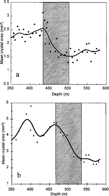
Fig. 2. Evolution of the mean cross-sectional area of crystals with depth from 350–580 m (a) at Dome C, EPICA and (b) at "old"Dome C (Reference Duval and LoriusDuval and Lorius, 1980). The continuous lines represent the data splines smoothing and the shaded area indicates the zone of the crystal-size decrease.
After this marked decrease, the crystal size seems to increase again in the deepest part of the core, supposedly within the Last Glacial.
4. Size Distributions
The shape of the grain-size distribution is another important parameter to characterize grain-growth or recrystallization processes in crystalline materials (see, e.g., Reference AtkinsonAtkinson, 1988 or Reference RalphRalph, 1990). It is customary to plot size distributions in terms of normalized grain "radius", R/Rm, where R can be calculated, for example, as the square root of a cross-sectional area, and Rm is the mean radius (see, e.g., Reference Anderson, Grest and SrolovitzAnderson and others, 1989). In material science, one classically divides the processes of grain growth into two types: normal and abnormal (Reference RalphRalph, 1990). Normal grain growth is characterized by a grain-size distribution remaining the same shape (typically log-normal) with time (Reference AtkinsonAtkinson, 1988; Reference RalphRalph, 1990).
A typical crystal-size distribution is shown in Figure 3a. The experimental histogram fits a log-normal distribution well. Similar histograms were extracted from each thin section along the whole core between 100 m and 580 m. Log-normal distributions were systematically observed. In a first approximation, the shape of the normalized size distribution is independent of depth (see below); all grain-size data at all depths together (>20 000 grains) are log-normally distributed (Fig. 3b).
Fig. 3. Relative gram radius (R/Rm) determined from cross-sectional analysis: experimental data are shown as histograms and fitted with a log-normal distribution, (a) Dataset corresponding to 492 m depth (average value of hi R/Rm = –0.22; std dev. = 0.49). (b) Dataset corresponding to all depths together (average value of hi R/Rm = –0.26; std dev. = 0.53).
A log-normal distribution is fully characterized by two independent parameters: the average value and standard deviation of ln(R/Rm). The evolution of these two parameters with depth is plotted in Figure 4a and b, respectively. The range of variation is narrow in both cases (see above and Fig. 3b). This is illustrated in Figure 5 which shows the most different log-normal distributions observed are, indeed, very close. This strongly argues for a normal grain-growth process for shallow polar ice. An abnormal grain growth would have been characterized by a second maximum in the grain-size distribution at large grain-size (see, e.g., Reference RalphRalph, 1990), never observed during this work.
Fig. 4. Evolution of the two independent parameters characterizing the log-normal distributions fitting the experimental histogram (In R/Rm). Average value (a) and standard deviation (b) of hi R/Rm are plotted vs depth. The dashed lines indicate the limits of the grain-size transition defined in Figure 2.
Fig. 5. Plots of the most different log-normal distributions fitting the experimental histograms of the relative grain radius. Continuous line is distribution corresponding to the beginning of the transition zone (average value of hi R/Rm = –0.35; std dev. = 0.65). Dashed line is distribution corresponding to the end of the transition zone (average value of hi R/Rm = –0.22; std dev. =0.51).
However, within these narrow ranges of variation, significant trends can be detected, especially during the decrease of the mean grain-size previously associated with a climatic transition. The average value and standard deviation of ln(R/Rm) follow inverse trends throughout the entire depth.
Ongoing detailed analyses of the variations of crystal-size distributions will help reveal the very nature of the grain-growth process in polar ice and especially the role of impurities (bubbles, dust, dissolved impurities; Reference Alley, Perepezko and BentleyAlley and others, 1986) on grain-boundary migration.
5. Shape Anisotropy
In order to show a possible anisotropy of grain shape, the ratio between the mean linear intercept along the horizontal (X) direction and the mean linear intercept along the vertical (Z) direction, ![]() has been calculated on vertical thin sections (Fig. 6). Estimations of
has been calculated on vertical thin sections (Fig. 6). Estimations of ![]() and
and ![]() were performed automatically with a line crossing the image each two pixels, i.e. 96.2 Mm. This ratio is systematically larger than 1, which means that the grains are flattened along the horizontal plane.
were performed automatically with a line crossing the image each two pixels, i.e. 96.2 Mm. This ratio is systematically larger than 1, which means that the grains are flattened along the horizontal plane.
Fig. 6. Evolution of the vertical-shape anisotropy (ratio between the mean linear intercept along the horizontal direction and the mean linear intercept along the vertical) with depth.
Flattening seems to increase with depth, from about 1.05 at 100 m to about 1.19 at 580 m. This corresponds to a flattening of roughly 13% over 480 m. Using the chronology given by Reference Lorius, Merlivat, Jouzel and PourchetLorius and others (1979) for the "old" Dome C, corrected by a 10% decrease of the accumulation rate (see section 3), one can estimate from this flattening a vertical strain rate of 0.13/ 13 000 yr = 1.00 × 10⁻⁵ yr−1. This is in good agreement with a simple estimate of this strain rate based on an equilibrium hypothesis for the ice sheet. At equilibrium, i.e. a constant thickness of the ice sheet, a 34 mm accumulation of ice (accumulation rate given by Reference Lorius, Merlivat, Jouzel and PourchetLorius and others (1979)) for the "old" Dome C corrected by a 10% decrease (see section 3)) is spread each year over a 3200 m deep ice column leading to a strain rate of 3.4/3200 = 1.04 × l0−5 yr−1. This agreement indirectly validates the hypothesis of homogeneity of the strain rate through the full ice thickness, used for the second estimate.
6. Conclusion
Experimental results on the ice microstructure (crystals size and shape) from the EPICA ice core at Dome Concordia have been obtained from image analysis of thin sections prepared during the first two field seasons (1997/98 and 1998/ 99). A novel digital-image processor developed at LGGE (Reference Gay and WeissGay and Weiss, in press) allowed the extraction not only of the mean value of the crystal size, but also size distributions and shape anisotropy
The mean crystal-size profile as well as crystal-size distributions reveal normal grain growth up to 430 m. Between 430 m and 500 m, a marked decrease of crystal size is observed and compared with similar trend obtained in the "old" Dome G ice core formerly associated with the Holocene/LGM transition (Reference Duval and LoriusDuval and Lorius, 1980). This seems to indicate a slightly lower accumulation rate (by φ10%) at Dome G. An increasing flattening of crystal shape is observed with depth. This enabled the vertical strain rate of the shallow part of the ice sheet to be estimated.
Completion of these preliminary experimental results will allow a better understanding of the physics of crystal growth and recrystallization processes in polar ice. Numerous different morphological and topological parameters will be extracted easily using our digital-image processing of the continuous thin section of the EPICA ice core. The effect on ice microstructure of parameters such as temperature, impurities content or stress-strain fields could be studied in order to use ice microstructure as a climatic record and to improve knowledge of the flow of ice sheets.
Acknowledgements
This work is a contribution to the "European Project for Ice Coring in Antarctica", a joint European Science Foundation ESF/European Commission (EC) scientific program, funded by the EC under the Environment and Climate Programme (1994–98) contract ENV4-CT95-0074 and by national contributions from Belgium, Denmark, France, Germany, Italy, The Netherlands, Norway, Sweden, Switzerland and the United Kingdom.
We would like to thank A. Manouvrier for technical assistance.


