


1 Introduction
Recent years have seen a number of breakthroughs in the classification of
 $C^*$
-algebras by K-theoretic invariants. For separable simple unital
$C^*$
-algebras by K-theoretic invariants. For separable simple unital
 $C^*$
-algebras A which have finite nuclear dimension and satisfy the Universal Coefficient Theorem of [Reference Rosenberg and SchochetRS87], the Elliott invariant (consisting of the ordered K-theory of A, its trace simplex, and the pairing between traces and
$C^*$
-algebras A which have finite nuclear dimension and satisfy the Universal Coefficient Theorem of [Reference Rosenberg and SchochetRS87], the Elliott invariant (consisting of the ordered K-theory of A, its trace simplex, and the pairing between traces and
 $K_0(A)$
) is a classifying invariant [Reference Tikuisis, White and WinterTWW17, Reference Elliott, Gong, Lin and NiuEGLN15, Reference Gong, Lin and NiuGLN21b, Reference Gong, Lin and NiuGLN21a]: two such
$K_0(A)$
) is a classifying invariant [Reference Tikuisis, White and WinterTWW17, Reference Elliott, Gong, Lin and NiuEGLN15, Reference Gong, Lin and NiuGLN21b, Reference Gong, Lin and NiuGLN21a]: two such
 $C^*$
-algebras
$C^*$
-algebras
 $A, B$
are isomorphic if and only if their Elliott invariants are isomorphic. Work has already begun [Reference Elliott, Gong, Lin and NiuEGLN20, Reference Gong and LinGL20] on expanding these results to the nonunital setting.
$A, B$
are isomorphic if and only if their Elliott invariants are isomorphic. Work has already begun [Reference Elliott, Gong, Lin and NiuEGLN20, Reference Gong and LinGL20] on expanding these results to the nonunital setting.
The Cuntz–Krieger algebras
 $\mathcal O_A$
[Reference Cuntz and KriegerCK80] associated with irreducible matrices A were one of the early classes of
$\mathcal O_A$
[Reference Cuntz and KriegerCK80] associated with irreducible matrices A were one of the early classes of
 $C^*$
-algebras for which K-theory was shown to be a classifying invariant [Reference Cuntz and KriegerCK80, Reference FranksFra84, Reference RørdamRø95]. When A is not irreducible,
$C^*$
-algebras for which K-theory was shown to be a classifying invariant [Reference Cuntz and KriegerCK80, Reference FranksFra84, Reference RørdamRø95]. When A is not irreducible,
 $\mathcal O_A$
is not simple, leaving these
$\mathcal O_A$
is not simple, leaving these
 $C^*$
-algebras outside the scope of the Elliott classification program. However, the proof of the K-theoretic classification of simple Cuntz–Krieger algebras draws heavily on the dynamical characterization of Cuntz–Krieger algebras as arising from one-sided shifts of finite type [Reference Cuntz and KriegerCK80]. As this dynamical characterization holds in the nonsimple case as well, Cuntz–Krieger algebras were a natural setting for a first foray into classification of nonsimple
$C^*$
-algebras outside the scope of the Elliott classification program. However, the proof of the K-theoretic classification of simple Cuntz–Krieger algebras draws heavily on the dynamical characterization of Cuntz–Krieger algebras as arising from one-sided shifts of finite type [Reference Cuntz and KriegerCK80]. As this dynamical characterization holds in the nonsimple case as well, Cuntz–Krieger algebras were a natural setting for a first foray into classification of nonsimple
 $C^*$
-algebras, and many classes of nonsimple Cuntz–Krieger algebras were classified in [Reference RestorffRes06, Reference Eilers and TomfordeET10, Reference SørensenSø13, Reference Eilers, Restorff, Ruiz and SørensenERRS18]. Indeed, recent work of Eilers et al. [Reference Eilers, Restorff, Ruiz and SørensenERRS16] completes this classification.
$C^*$
-algebras, and many classes of nonsimple Cuntz–Krieger algebras were classified in [Reference RestorffRes06, Reference Eilers and TomfordeET10, Reference SørensenSø13, Reference Eilers, Restorff, Ruiz and SørensenERRS18]. Indeed, recent work of Eilers et al. [Reference Eilers, Restorff, Ruiz and SørensenERRS16] completes this classification.
Interpreting A as the adjacency matrix of a directed graph
 $E_A$
, we have a canonical isomorphism
$E_A$
, we have a canonical isomorphism
 $\mathcal O_A \cong C^*(E_A)$
. Using this perspective, as well as techniques from symbolic dynamics [Reference HuangHua96, Reference BoyleBoy02, Reference Boyle and HuangBH], Eilers et al. obtained both a K-theoretic and a graph-theoretic classification of unital graph
$\mathcal O_A \cong C^*(E_A)$
. Using this perspective, as well as techniques from symbolic dynamics [Reference HuangHua96, Reference BoyleBoy02, Reference Boyle and HuangBH], Eilers et al. obtained both a K-theoretic and a graph-theoretic classification of unital graph
 $C^*$
-algebras. To be precise, Sørensen [Reference SørensenSø13] identifies five “moves” on directed graphs E which preserve the stable isomorphism class of
$C^*$
-algebras. To be precise, Sørensen [Reference SørensenSø13] identifies five “moves” on directed graphs E which preserve the stable isomorphism class of
 $C^*(E)$
, and shows that in fact these moves generate the equivalence relation
$C^*(E)$
, and shows that in fact these moves generate the equivalence relation
 $$ \begin{align} E \sim F \iff C^*(E) \otimes \mathcal K \cong C^*(F) \otimes \mathcal K \end{align} $$
among graphs with simple unital
 $C^*$
-algebras. In [Reference Eilers, Restorff, Ruiz and SørensenERRS18], Eilers et al. confirmed that these five moves are not sufficient to generate the equivalence relation (1.1) on the class of all finite graphs. However, [Reference Eilers, Restorff, Ruiz and SørensenERRS16] identifies a sixth operation on directed graphs which preserves the equivalence relation (1.1), and uses filtered K-theory to show that, among graphs with finitely many vertices, these six moves generate the equivalence relation (1.1). That is, an isomorphism
$C^*$
-algebras. In [Reference Eilers, Restorff, Ruiz and SørensenERRS18], Eilers et al. confirmed that these five moves are not sufficient to generate the equivalence relation (1.1) on the class of all finite graphs. However, [Reference Eilers, Restorff, Ruiz and SørensenERRS16] identifies a sixth operation on directed graphs which preserves the equivalence relation (1.1), and uses filtered K-theory to show that, among graphs with finitely many vertices, these six moves generate the equivalence relation (1.1). That is, an isomorphism
 $C^*(E) \otimes \mathcal {K} \cong C^*(F) \otimes \mathcal {K}$
can only exist if we can pass from E to F by a finite sequence of these six moves and their inverses. Eilers et al. also showed in [Reference Eilers, Restorff, Ruiz and SørensenERRS16] that isomorphism of two unital graph
$C^*(E) \otimes \mathcal {K} \cong C^*(F) \otimes \mathcal {K}$
can only exist if we can pass from E to F by a finite sequence of these six moves and their inverses. Eilers et al. also showed in [Reference Eilers, Restorff, Ruiz and SørensenERRS16] that isomorphism of two unital graph
 $C^*$
-algebras
$C^*$
-algebras
 $C^*(E), C^*(F)$
is equivalent to the existence of an order-preserving isomorphism of the filtered K-theory of
$C^*(E), C^*(F)$
is equivalent to the existence of an order-preserving isomorphism of the filtered K-theory of
 $C^*(E)$
and
$C^*(E)$
and
 $C^*(F)$
.
$C^*(F)$
.
The K-theory of a graph
 $C^*$
-algebra [Reference CuntzCun81, Reference Bates, Hong, Raeburn and SzymańskiBHRS02] dictates that if
$C^*$
-algebra [Reference CuntzCun81, Reference Bates, Hong, Raeburn and SzymańskiBHRS02] dictates that if
 $C^*(E)$
is simple, it is either approximately finite-dimensional or purely infinite. Kumjian and Pask developed the theory of higher-rank graphs, or k-graphs, in [Reference Kumjian and PaskKP00] to provide a broader range of combinatorial examples of
$C^*(E)$
is simple, it is either approximately finite-dimensional or purely infinite. Kumjian and Pask developed the theory of higher-rank graphs, or k-graphs, in [Reference Kumjian and PaskKP00] to provide a broader range of combinatorial examples of
 $C^*$
-algebras. Formally, a k-graph
$C^*$
-algebras. Formally, a k-graph
 $\Lambda $
is a countable category with a functor
$\Lambda $
is a countable category with a functor
 $d: \Lambda \to {\mathbb N}^k$
satisfying a factorization property (see Definition 2.0.1 below). However, k-graphs are also closely linked to buildings [Reference Robertson and StegerRS99, Reference Konter and VdovinaKV15] and to higher-rank shifts of finite type via textile systems [Reference Johnson and MaddenJM99]. The graph-theoretic inspiration for higher-rank graphs was made precise by Hazlewood et al. [Reference Hazlewood, Raeburn, Sims and WebsterHRSW13], who detailed in [Reference Hazlewood, Raeburn, Sims and WebsterHRSW13, Theorems 4.4 and 4.5] the correspondence between higher-rank graphs on the one hand, and on the other hand, edge-colored directed graphs with an equivalence relation on their category of paths. In this perspective, the factorization property of a k-graph is encoded in the set of “commuting squares,” or length-2 paths
$d: \Lambda \to {\mathbb N}^k$
satisfying a factorization property (see Definition 2.0.1 below). However, k-graphs are also closely linked to buildings [Reference Robertson and StegerRS99, Reference Konter and VdovinaKV15] and to higher-rank shifts of finite type via textile systems [Reference Johnson and MaddenJM99]. The graph-theoretic inspiration for higher-rank graphs was made precise by Hazlewood et al. [Reference Hazlewood, Raeburn, Sims and WebsterHRSW13], who detailed in [Reference Hazlewood, Raeburn, Sims and WebsterHRSW13, Theorems 4.4 and 4.5] the correspondence between higher-rank graphs on the one hand, and on the other hand, edge-colored directed graphs with an equivalence relation on their category of paths. In this perspective, the factorization property of a k-graph is encoded in the set of “commuting squares,” or length-2 paths
 $ab \sim cd$
which are equivalent in the edge-colored directed graph.
$ab \sim cd$
which are equivalent in the edge-colored directed graph.
The paper at hand constitutes a first step toward extending the geometric classification of graph
 $C^*$
-algebras to the setting of higher-rank graphs. Taking inspiration from [Reference DrinenDri99, Reference Bates and PaskBP04, Reference Crisp and GowCG06, Reference SørensenSø13], we identify four moves (sink deletion, in-splitting, reduction, and delay) on row-finite, source-free k-graphs
$C^*$
-algebras to the setting of higher-rank graphs. Taking inspiration from [Reference DrinenDri99, Reference Bates and PaskBP04, Reference Crisp and GowCG06, Reference SørensenSø13], we identify four moves (sink deletion, in-splitting, reduction, and delay) on row-finite, source-free k-graphs
 $\Lambda $
which preserve the Morita equivalence class of
$\Lambda $
which preserve the Morita equivalence class of
 $C^*(\Lambda )$
. These moves for k-graphs were inspired by their analogs for directed graphs, and therefore involve adding or removing edges and vertices in
$C^*(\Lambda )$
. These moves for k-graphs were inspired by their analogs for directed graphs, and therefore involve adding or removing edges and vertices in
 $\Lambda $
. Performing such a move on a k-graph affects the factorization property, though, as length-2 paths may become longer or shorter. Thus, geometric classification in the k-graph setting faces a new technical hurdle: one must identify how to adjust the factorization property after each move, so that the resulting object is still a k-graph.
$\Lambda $
. Performing such a move on a k-graph affects the factorization property, though, as length-2 paths may become longer or shorter. Thus, geometric classification in the k-graph setting faces a new technical hurdle: one must identify how to adjust the factorization property after each move, so that the resulting object is still a k-graph.
As discussed in the introduction to [Reference Bates and PaskBP04], the moves of in-splitting and delay originate in symbolic dynamics. For shifts of finite type, the natural relations of conjugacy and flow equivalence [Reference Parry and SullivanPS75] are generated by matrix operations which, when translated into the graph setting, correspond to the moves of in-splitting, out-splitting, and delay. (See [Reference Lind and MarcusLM95, Sections 2.3 and 2.4] for more details.) For directed graphs, the analogs (S) of sink deletion and (R) of reduction were first isolated by Sørensen [Reference SørensenSø13], drawing on the very general framework given in [Reference Crisp and GowCG06] for modifying a directed graph without changing its Morita equivalence class. The main result of [Reference SørensenSø13, Theorem 4.3] establishes that, for directed graphs
 $E, F$
with finitely many vertices such that
$E, F$
with finitely many vertices such that
 $C^*(E)$
and
$C^*(E)$
and
 $C^*(F)$
are simple, any stable isomorphism
$C^*(F)$
are simple, any stable isomorphism
 $C^*(E) \otimes \mathcal K \cong C^*(F) \otimes \mathcal K$
must arise from a finite sequence of in-splittings, out-splittings, Cuntz splice, the moves (S) and (R), and their inverses. As mentioned above, subsequent work by Eilers et al. [Reference Eilers, Restorff, Ruiz and SørensenERRS18, Reference Eilers, Restorff, Ruiz and SørensenERRS16] has extended this geometric analysis of the equivalence relation (1.1) to cover many classes of nonsimple graph
$C^*(E) \otimes \mathcal K \cong C^*(F) \otimes \mathcal K$
must arise from a finite sequence of in-splittings, out-splittings, Cuntz splice, the moves (S) and (R), and their inverses. As mentioned above, subsequent work by Eilers et al. [Reference Eilers, Restorff, Ruiz and SørensenERRS18, Reference Eilers, Restorff, Ruiz and SørensenERRS16] has extended this geometric analysis of the equivalence relation (1.1) to cover many classes of nonsimple graph
 $C^*$
-algebras.
$C^*$
-algebras.
We now outline the structure of this paper. The picture of higher-rank graphs as arising from edge-colored directed graphs underlies our work in this paper, and so we take some pains in Section 2 to assure the reader of the equivalence between our approach to k-graphs and the more common category-theoretic perspective. To obtain our Morita equivalence results, we rely heavily on a generalization of the gauge-invariant uniqueness theorem for k-graphs [Reference Kumjian and PaskKP00], and on Allen’s results [Reference AllenAll08] about corners in higher-rank graphs, so we also review these notions in Section 2.
Each of Sections 3–6 is dedicated to one of our four Morita equivalence-preserving moves on k-graphs. For each move, we first ensure that its output is a k-graph, and then we show that the resulting k-graph
 $C^*$
-algebra is Morita equivalent to our original
$C^*$
-algebra is Morita equivalent to our original
 $C^*$
-algebra. We begin with in-splitting in Section 3. We first describe conditions under which we can “in-split” a k-graph at a vertex v—that is, create two copies of v and divide the edges with range v among the two copies—in such a way that the resulting object is still a k-graph (Theorem 3.8). Theorem 3.9 then establishes that in-splitting produces a
$C^*$
-algebra. We begin with in-splitting in Section 3. We first describe conditions under which we can “in-split” a k-graph at a vertex v—that is, create two copies of v and divide the edges with range v among the two copies—in such a way that the resulting object is still a k-graph (Theorem 3.8). Theorem 3.9 then establishes that in-splitting produces a
 $C^*$
-algebra which is isomorphic to our original one, not merely Morita equivalent. Section 4 studies the move of “delaying” an edge by breaking it into two edges. In order to delay an edge in a k-graph, the k-graph’s factorization rule also forces us to delay many of the edges of the same color. In Theorem 4.1, we show that this move results in a k-graph. Moreover, its
$C^*$
-algebra which is isomorphic to our original one, not merely Morita equivalent. Section 4 studies the move of “delaying” an edge by breaking it into two edges. In order to delay an edge in a k-graph, the k-graph’s factorization rule also forces us to delay many of the edges of the same color. In Theorem 4.1, we show that this move results in a k-graph. Moreover, its
 $C^*$
-algebra is Morita equivalent to that of our original k-graph (Theorem 4.2). In Section 5, we show in Theorem 5.4 that if a vertex is a sink—that is, it emits no edges of a given color—then after deleting the sink and all incident edges, we are still left with a k-graph. The fact that this move does not change the Morita equivalence class of the k-graph
$C^*$
-algebra is Morita equivalent to that of our original k-graph (Theorem 4.2). In Section 5, we show in Theorem 5.4 that if a vertex is a sink—that is, it emits no edges of a given color—then after deleting the sink and all incident edges, we are still left with a k-graph. The fact that this move does not change the Morita equivalence class of the k-graph
 $C^*$
-algebra is established in Theorem 5.5. Finally, we turn to “reduction” in Section 6, where we identify when contraction (reduction) of a “complete edge” (see Definition 6.0.1) in a k-graph produces a k-graph (Theorem 6.3). In this case, the
$C^*$
-algebra is established in Theorem 5.5. Finally, we turn to “reduction” in Section 6, where we identify when contraction (reduction) of a “complete edge” (see Definition 6.0.1) in a k-graph produces a k-graph (Theorem 6.3). In this case, the
 $C^*$
-algebra of the resulting k-graph is always Morita equivalent to the original k-graph
$C^*$
-algebra of the resulting k-graph is always Morita equivalent to the original k-graph
 $C^*$
-algebra, by Theorem 6.4. Throughout the paper, we include examples showcasing the moves and indicating the necessity of our hypotheses.
$C^*$
-algebra, by Theorem 6.4. Throughout the paper, we include examples showcasing the moves and indicating the necessity of our hypotheses.
2 Notation
Fix an integer
 $k \ge 1$
. As our main objects of study in this paper are k-graphs (higher-rank graphs), we begin by recalling their definition. First, however, we specify that throughout this paper we regard
$k \ge 1$
. As our main objects of study in this paper are k-graphs (higher-rank graphs), we begin by recalling their definition. First, however, we specify that throughout this paper we regard
 $0$
as an element of
$0$
as an element of
 $\mathbb {N}$
, and we view
$\mathbb {N}$
, and we view
 ${\mathbb N}^k$
as a category, with composition of morphisms given by addition. Consequently,
${\mathbb N}^k$
as a category, with composition of morphisms given by addition. Consequently,
 $\mathbb {N}^k$
has one object (namely
$\mathbb {N}^k$
has one object (namely
 $(0, \ldots , 0)$
). For
$(0, \ldots , 0)$
). For
 $n = \sum _{i=1}^k n_i e_i \in {\mathbb N}^k,$
we write
$n = \sum _{i=1}^k n_i e_i \in {\mathbb N}^k,$
we write
 $|n| = \sum _i n_i$
.
$|n| = \sum _i n_i$
.
Definition 2.0.1 [Reference Kumjian and PaskKP00, Definition 1.1]
Let
 $\Lambda $
be a countable category and
$\Lambda $
be a countable category and
 $d: \Lambda \to \mathbb {N}^k$
a functor. If
$d: \Lambda \to \mathbb {N}^k$
a functor. If
 $(\Lambda , d)$
satisfies the factorization rule—that is, for every morphism
$(\Lambda , d)$
satisfies the factorization rule—that is, for every morphism
 $\lambda \in \Lambda $
and
$\lambda \in \Lambda $
and
 $n,m \in \mathbb {N}^k$
such that
$n,m \in \mathbb {N}^k$
such that
 $d(\lambda ) = n + m$
, there exist unique
$d(\lambda ) = n + m$
, there exist unique
 $\mu , \nu \in \Lambda $
such that
$\mu , \nu \in \Lambda $
such that
 $d(\mu ) = m$
,
$d(\mu ) = m$
,
 $d(\nu ) = n$
, and
$d(\nu ) = n$
, and
 $\lambda = \mu \nu $
—then
$\lambda = \mu \nu $
—then
 $(\Lambda ,d)$
is a k-graph.
$(\Lambda ,d)$
is a k-graph.
We write
 $\Lambda ^1 = \{ \lambda \in \Lambda : |d(\lambda )|=1\}$
and
$\Lambda ^1 = \{ \lambda \in \Lambda : |d(\lambda )|=1\}$
and
 $\Lambda ^0 = d^{-1}(0)$
. If
$\Lambda ^0 = d^{-1}(0)$
. If
 $e \in \Lambda ^1$
, we say e is an edge of
$e \in \Lambda ^1$
, we say e is an edge of
 $\Lambda $
, and
$\Lambda $
, and
 $\Lambda ^0$
is the set of vertices of
$\Lambda ^0$
is the set of vertices of
 $\Lambda $
.
$\Lambda $
.
Observe that the factorization rule guarantees, for each
 $\lambda \in \Lambda $
, the existence of unique
$\lambda \in \Lambda $
, the existence of unique
 $v, w \in \Lambda ^0$
such that
$v, w \in \Lambda ^0$
such that
 $v \lambda w = \lambda ;$
we will write
$v \lambda w = \lambda ;$
we will write
 $r(\lambda )$
for v and
$r(\lambda )$
for v and
 $s(\lambda )$
for w. Similarly, we write
$s(\lambda )$
for w. Similarly, we write
 $$ \begin{align*} v \Lambda= \{ \lambda \in \Lambda: r(\lambda) = v\} \quad \text{ and } \quad v\Lambda^n = \{ \lambda \in v \Lambda: d(\lambda) = n\}\end{align*} $$
for any
 $n\in \mathbb {N}^k$
. The sets
$n\in \mathbb {N}^k$
. The sets
 $\Lambda w, \Lambda ^n w$
are defined analogously.
$\Lambda w, \Lambda ^n w$
are defined analogously.
Our reason for the convention that the source of a morphism in
 $\Lambda $
lies on its right, and its range lies to the left, arises from the Cuntz–Krieger relations used to define k-graph
$\Lambda $
lies on its right, and its range lies to the left, arises from the Cuntz–Krieger relations used to define k-graph
 $C^*$
-algebras; see Definition 2.1.1 and Remark 2.2 below.
$C^*$
-algebras; see Definition 2.1.1 and Remark 2.2 below.
We now briefly describe how to model k-graphs using k-colored graphs as we use this framework extensively for our constructions. Following [Reference Hazlewood, Raeburn, Sims and WebsterHRSW13], we let
 $G = (G^0, G^1, r, s)$
denote a directed graph with
$G = (G^0, G^1, r, s)$
denote a directed graph with
 $G^0$
its set of vertices and
$G^0$
its set of vertices and
 $G^1$
its set of edges;
$G^1$
its set of edges;
 $r, s: G^1 \to G^0$
are the range and source map, respectively. For an integer
$r, s: G^1 \to G^0$
are the range and source map, respectively. For an integer
 $n \ge 2$
, let
$n \ge 2$
, let
 $G^n$
denote the paths of length n in G. By a slight abuse of notation, if
$G^n$
denote the paths of length n in G. By a slight abuse of notation, if
 $\delta \in G^n$
, we will write
$\delta \in G^n$
, we will write
 $|\delta | := n$
.
$|\delta | := n$
.
We now color the graph G by assigning to each edge one of the standard basis vectors,
 $e_i$
, of
$e_i$
, of
 ${\mathbb N}^k$
and let
${\mathbb N}^k$
and let
 $G^{e_i}$
be the set of edges assigned to
$G^{e_i}$
be the set of edges assigned to
 $e_i$
, so that
$e_i$
, so that
 $G^1 = \bigcup _{i=1}^k G^{e_i}$
. The path category,
$G^1 = \bigcup _{i=1}^k G^{e_i}$
. The path category,
 $G^* = \bigcup _{n\in \mathbb {N}} G^n$
, may now be equipped with a degree functor
$G^* = \bigcup _{n\in \mathbb {N}} G^n$
, may now be equipped with a degree functor
 $d: G^* \to {\mathbb N}^k$
, given on the vertices by
$d: G^* \to {\mathbb N}^k$
, given on the vertices by
 $d(v) = 0$
for all
$d(v) = 0$
for all
 $v \in G^0$
, and on the edges by
$v \in G^0$
, and on the edges by
 $d(f) = e_i$
if f was assigned the basis vector
$d(f) = e_i$
if f was assigned the basis vector
 $e_i$
. On longer paths, d is extended to be additive:
$e_i$
. On longer paths, d is extended to be additive:
 $d(f_n \cdots f_1) = \sum _{i=1}^n d(f_i)$
. (Our reason for this enumeration of the edges in a path is that in a k-graph, by Definition 2.0.1, we have
$d(f_n \cdots f_1) = \sum _{i=1}^n d(f_i)$
. (Our reason for this enumeration of the edges in a path is that in a k-graph, by Definition 2.0.1, we have
 $s(f_i) = r(f_{i-1})$
whenever
$s(f_i) = r(f_{i-1})$
whenever
 $f_i f_{i-1}$
is a well-defined product of morphisms in a k-graph. Consistency with this definition requires that the right-most edge in a path,
$f_i f_{i-1}$
is a well-defined product of morphisms in a k-graph. Consistency with this definition requires that the right-most edge in a path,
 $f_1$
, denotes the path’s initial edge and the left-most edge,
$f_1$
, denotes the path’s initial edge and the left-most edge,
 $f_n$
, its final edge.) As usual, the range and source maps
$f_n$
, its final edge.) As usual, the range and source maps
 $r,s: G^1 \to G^0$
extend to well-defined maps from
$r,s: G^1 \to G^0$
extend to well-defined maps from
 $G^*$
to
$G^*$
to
 $G^0$
, which we continue to denote by r and s.
$G^0$
, which we continue to denote by r and s.
Theorem 4.5 of [Reference Hazlewood, Raeburn, Sims and WebsterHRSW13] establishes that if G is a k-colored graph as described above, then
 $\Lambda = G^* / \sim $
is a k-graph for any
$\Lambda = G^* / \sim $
is a k-graph for any
 $(r,s,d)$
-preserving equivalence relation
$(r,s,d)$
-preserving equivalence relation
 $\sim $
on
$\sim $
on
 $G^*$
which also satisfies
$G^*$
which also satisfies
-
(KG0) If
 $\lambda \in G^*$
is a path such that
$\lambda = \lambda _2 \lambda _1$
, then
$[\lambda ] = [p_2 p_1]$
whenever
$p_1 \in [\lambda _1]$
and
$p_2 \in [\lambda _2]$
.
$\lambda \in G^*$
is a path such that
$\lambda = \lambda _2 \lambda _1$
, then
$[\lambda ] = [p_2 p_1]$
whenever
$p_1 \in [\lambda _1]$
and
$p_2 \in [\lambda _2]$
. -
(KG1) If
$f,g \in G^1$
are edges, then
$f \sim g \Leftrightarrow f = g$
. -
(KG2) Completeness: For every
$\mu = \mu _2 \mu _1 \in G^2$
such that
$d(\mu _1) = e_i$
,
$d(\mu _2) = e_j$
, there exists a unique
$\nu = \nu _2 \nu _1 \in G^2$
such that
$d(\nu _1) = e_j$
,
$d(\nu _2) = e_i$
and
$\mu \sim \nu $
. -
(KG3) Associativity: For any
$e_i$
–
$e_j$
–
$e_\ell $
path
$abc \in G^3$
with
$i,j,\ell $
all distinct, the
$e_\ell $
–
$e_j$
–
$e_i$
paths
$hjg, nrq$
constructed via the following two routes are equal.


-
Route 1: Let
$ab \sim de$
, so
$abc \sim dec$
.Let
$ec \sim fg$
, so
$abc \sim dfg$
.Let
$df \sim hj$
, so
$abc \sim hjg$
. -
Route 2: Let
$bc \sim km$
, so
$abc \sim akm$
.Let
$ak \sim np$
, so
$abc \sim npm$
.Let
$pm \sim rq$
, so
$abc \sim nrq$
.


In fact, [Reference Hazlewood, Raeburn, Sims and WebsterHRSW13, Theorem 4.4] shows that every k-graph arises in this way. That is, given a k-graph
 $\Lambda $
, we obtain a directed graph G by setting
$\Lambda $
, we obtain a directed graph G by setting
 $G^0 = \Lambda ^0, G^1 = \Lambda ^1$
. (This justifies our decision to call
$G^0 = \Lambda ^0, G^1 = \Lambda ^1$
. (This justifies our decision to call
 $\Lambda ^0$
the vertices of
$\Lambda ^0$
the vertices of
 $\Lambda $
and
$\Lambda $
and
 $\Lambda ^1$
the edges of
$\Lambda ^1$
the edges of
 $\Lambda $
.) Transferring the degree map
$\Lambda $
.) Transferring the degree map
 $d: \Lambda \to \mathbb {N}^k$
to G makes G a k-colored graph; we obtain an equivalence relation on
$d: \Lambda \to \mathbb {N}^k$
to G makes G a k-colored graph; we obtain an equivalence relation on
 $G^*$
by setting
$G^*$
by setting
 $\lambda \sim \mu $
if the paths
$\lambda \sim \mu $
if the paths
 $\lambda , \mu $
represent the same morphism in
$\lambda , \mu $
represent the same morphism in
 $\Lambda $
. The factorization rule in
$\Lambda $
. The factorization rule in
 $\Lambda $
then implies that
$\Lambda $
then implies that
 $\sim $
satisfies (KG0)–(KG3).
$\sim $
satisfies (KG0)–(KG3).
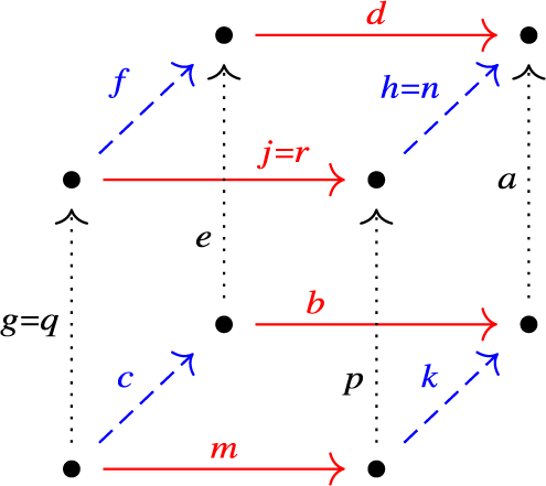
Figure 1: (KG3).
In this paper, we fully exploit the equivalence between k-colored directed graphs with equivalence relations on the one hand, and k-graphs on the other hand. Our general strategy will be to define a move M on a k-graph
 $\Lambda $
in terms of its impact on the 1-skeleton G and the equivalence relation
$\Lambda $
in terms of its impact on the 1-skeleton G and the equivalence relation
 $\sim $
which give rise to
$\sim $
which give rise to
 $\Lambda $
. This produces a new colored graph
$\Lambda $
. This produces a new colored graph
 $G_M$
with a new equivalence relation
$G_M$
with a new equivalence relation
 $\sim _M$
, which we then show satisfies (KG0)–(KG3), so that the quotient
$\sim _M$
, which we then show satisfies (KG0)–(KG3), so that the quotient
 $G_M/\sim _M$
is a new k-graph
$G_M/\sim _M$
is a new k-graph
 $\Lambda _M$
.
$\Lambda _M$
.
For
 $\lambda \in G^*$
, we notate its equivalence class under
$\lambda \in G^*$
, we notate its equivalence class under
 $\sim $
as
$\sim $
as
 $[\lambda ] \in \Lambda $
. For
$[\lambda ] \in \Lambda $
. For
 $n \in \mathbb {N}^k$
, we write
$n \in \mathbb {N}^k$
, we write
 $$ \begin{align*}\Lambda^n = \{ [\lambda] \in \Lambda : d([\lambda]) = n \}.\end{align*} $$
For our purposes in this paper, we will also need an alternative characterization of the equivalence relations on
 $G^*$
which give rise to k-graphs. We begin by observing that an inductive application of the factorization rule of Definition 2.0.1 reveals that if
$G^*$
which give rise to k-graphs. We begin by observing that an inductive application of the factorization rule of Definition 2.0.1 reveals that if
 $\Lambda $
is a k-graph, then for any morphism
$\Lambda $
is a k-graph, then for any morphism
 $\lambda \in \Lambda $
and ordered n-tuple
$\lambda \in \Lambda $
and ordered n-tuple
 $(m_1, \dots , m_n)$
of elements of
$(m_1, \dots , m_n)$
of elements of
 $\mathbb {N}^k$
such that
$\mathbb {N}^k$
such that
 $|m_i| = 1$
for all i and
$|m_i| = 1$
for all i and
 $m_1 + \cdots + m_n = d(\lambda )$
, there is a unique set of edges
$m_1 + \cdots + m_n = d(\lambda )$
, there is a unique set of edges
 $\lambda _1, \dots , \lambda _n \in \Lambda ^1$
such that
$\lambda _1, \dots , \lambda _n \in \Lambda ^1$
such that
 $\lambda = \lambda _n \cdots \lambda _1$
where
$\lambda = \lambda _n \cdots \lambda _1$
where
 $d(\lambda _i) = m_i$
.
$d(\lambda _i) = m_i$
.
Definition 2.0.2 For a finite path
 $\lambda $
in an edge-colored directed graph G, let
$\lambda $
in an edge-colored directed graph G, let
 $\lambda _i$
denote the ith edge of
$\lambda _i$
denote the ith edge of
 $\lambda $
(counting from the source of
$\lambda $
(counting from the source of
 $\lambda $
). The color order of
$\lambda $
). The color order of
 $\lambda $
is the
$\lambda $
is the
 $|\lambda |$
-tuple
$|\lambda |$
-tuple
 $(d(\lambda _1), d(\lambda _2), \dots , d(\lambda _{|\lambda |}))$
.
$(d(\lambda _1), d(\lambda _2), \dots , d(\lambda _{|\lambda |}))$
.
This leads us to the following condition on an equivalence relation
 $\sim $
on
$\sim $
on
 $G^*$
:
$G^*$
:
-
(KG4) For each
$\lambda \in G^*$
and each permutation of the color order of
$\lambda $
, there is a unique path
$\mu \in [\lambda ]$
with the permuted color order.


Theorem 2.1 Let G be an edge-colored directed graph and suppose
 $\sim $
is an
$\sim $
is an
 $(r, s, d)$
-preserving equivalence relation on
$(r, s, d)$
-preserving equivalence relation on
 $G^*$
satisfying
$G^*$
satisfying
 $(KG0)$
. The relation
$(KG0)$
. The relation
 $\sim $
satisfies
$\sim $
satisfies
 $(KG1), (KG2)$
, and
$(KG1), (KG2)$
, and
 $(KG3)$
(and hence
$(KG3)$
(and hence
 $G^*/\sim $
is a k-graph) if and only if
$G^*/\sim $
is a k-graph) if and only if
 $\sim $
satisfies
$\sim $
satisfies
 $(KG4)$
.
$(KG4)$
.
Proof First, assume (KG0) and (KG4) hold for
 $\sim $
and consider an
$\sim $
and consider an
 $e_i$
–
$e_i$
–
 $e_j$
–
$e_j$
–
 $e_\ell $
path
$e_\ell $
path
 $\lambda \in G^3$
. Convert
$\lambda \in G^3$
. Convert
 $\lambda $
into two
$\lambda $
into two
 $e_\ell $
–
$e_\ell $
–
 $e_j$
–
$e_j$
–
 $e_i$
paths via the routes described in (KG3) and label them
$e_i$
paths via the routes described in (KG3) and label them
 $\mu $
and
$\mu $
and
 $\nu $
. Because
$\nu $
. Because
 $\mu \sim \lambda $
and
$\mu \sim \lambda $
and
 $\nu \sim \lambda $
by construction, the fact that
$\nu \sim \lambda $
by construction, the fact that
 $\sim $
is an equivalence relation implies that
$\sim $
is an equivalence relation implies that
 $\mu \sim \nu $
. Condition (KG4) and the fact that
$\mu \sim \nu $
. Condition (KG4) and the fact that
 $\mu , \nu $
have the same color order now give
$\mu , \nu $
have the same color order now give
 $\mu $
=
$\mu $
=
 $\nu $
. Thus, (KG3) holds. Similarly, if
$\nu $
. Thus, (KG3) holds. Similarly, if
 $\lambda \in G^2$
, then there exists a unique
$\lambda \in G^2$
, then there exists a unique
 $\mu \in [\lambda ]$
of each permuted color order. Thus, (KG2) holds. Finally, for
$\mu \in [\lambda ]$
of each permuted color order. Thus, (KG2) holds. Finally, for
 $e,f \in G^1$
, we have
$e,f \in G^1$
, we have
 $e \sim f \implies d(e) = d(f) \implies e = f$
, because each color order has a unique associated path. Also,
$e \sim f \implies d(e) = d(f) \implies e = f$
, because each color order has a unique associated path. Also,
 $e = f \implies e \sim f$
. Thus, (KG1) holds.
$e = f \implies e \sim f$
. Thus, (KG1) holds.
Now, assume
 $\sim $
satisfies (KG0), (KG1), (KG2), and (KG3). We know from [Reference Hazlewood, Raeburn, Sims and WebsterHRSW13, Theorem 4.5] that
$\sim $
satisfies (KG0), (KG1), (KG2), and (KG3). We know from [Reference Hazlewood, Raeburn, Sims and WebsterHRSW13, Theorem 4.5] that
 $\Lambda := G^* / \sim $
is a k-graph. Thus, fix
$\Lambda := G^* / \sim $
is a k-graph. Thus, fix
 $\delta \in G^*$
, and choose a sequence of basis vectors
$\delta \in G^*$
, and choose a sequence of basis vectors
 $(m_j)_{j=1}^{|\delta |},$
with
$(m_j)_{j=1}^{|\delta |},$
with
 $m_j \in \{ e_i\}_{i=1}^k$
for all j, such that
$m_j \in \{ e_i\}_{i=1}^k$
for all j, such that
 $d(\delta ) = \sum _{j = 1}^{|\delta |}m_{j}$
. An inductive application of the factorization rule of Definition 2.0.1 implies the existence of a unique path
$d(\delta ) = \sum _{j = 1}^{|\delta |}m_{j}$
. An inductive application of the factorization rule of Definition 2.0.1 implies the existence of a unique path
 $\gamma = \gamma _{|\delta |} \cdots \gamma _2 \gamma _1 \in [\delta ]$
where
$\gamma = \gamma _{|\delta |} \cdots \gamma _2 \gamma _1 \in [\delta ]$
where
 $d(\gamma _j) = m_j$
for every j. Because our ordering of the basis vectors
$d(\gamma _j) = m_j$
for every j. Because our ordering of the basis vectors
 $(m_1, \ldots , m_{|d(\lambda )|})$
was arbitrary, it follows that
$(m_1, \ldots , m_{|d(\lambda )|})$
was arbitrary, it follows that
 $\sim $
satisfies (KG4). ▪
$\sim $
satisfies (KG4). ▪
Notation 2.1.1 A k-graph
 $\Lambda $
is row-finite if for all
$\Lambda $
is row-finite if for all
 $v \in \Lambda ^0$
and all
$v \in \Lambda ^0$
and all
 $1 \leq i \leq k$
, we have
$1 \leq i \leq k$
, we have
 $| \{ \lambda \in \Lambda ^{e_i}: r(\lambda ) = v\}| < \infty .$
We say
$| \{ \lambda \in \Lambda ^{e_i}: r(\lambda ) = v\}| < \infty .$
We say
 $v \in \Lambda ^0$
is a source if there is i such that
$v \in \Lambda ^0$
is a source if there is i such that
 $r^{-1}(v) \cap \Lambda ^{e_{i}} = \emptyset $
.
$r^{-1}(v) \cap \Lambda ^{e_{i}} = \emptyset $
.
In this paper, we will focus exclusively on row-finite source-free k-graphs.
Definition 2.1.1 [Reference Kumjian and PaskKP00, Definition 1.5], [Reference Kumjian, Pask and SimsKPS12, Definition 7.4]
Let
 $\Lambda $
be a row-finite, source-free k-graph
$\Lambda $
be a row-finite, source-free k-graph
 $\Lambda $
. A Cuntz–Krieger
$\Lambda $
. A Cuntz–Krieger
 $\Lambda $
-family is a collection of projections
$\Lambda $
-family is a collection of projections
 $\{P_v: v \in \Lambda ^0\}$
and partial isometries
$\{P_v: v \in \Lambda ^0\}$
and partial isometries
 $\{ T_f: f \in \Lambda ^1\}$
satisfying the Cuntz–Krieger relations
$\{ T_f: f \in \Lambda ^1\}$
satisfying the Cuntz–Krieger relations
 $:$
$:$
-
(CK1) The projections
$P_v$
are mutually orthogonal. -
(CK2) If
$a, b, f, g \in \Lambda ^1$
satisfy
$af \sim gb $
, then
$T_a T_f = T_g T_b.$
-
(CK3) For any
$f \in \Lambda ^1$
, we have
$T_f^* T_f = P_{s(f)}.$
-
(CK4) For any
$v\in \Lambda ^0$
and any
$1 \leq i \leq k,$
we have
$\displaystyle P_v = \sum _{f: r(f) = v, d(f) = e_i}T_fT_f^*.$


There is a universal
 $C^*$
-algebra for these generators and relations, which is denoted
$C^*$
-algebra for these generators and relations, which is denoted
 $C^*(\Lambda ) = C^*(\{ p_v, t_f\})$
. For any Cuntz–Krieger
$C^*(\Lambda ) = C^*(\{ p_v, t_f\})$
. For any Cuntz–Krieger
 $\Lambda $
-family
$\Lambda $
-family
 $\{ P_v, T_f\}$
, we consequently have a surjective
$\{ P_v, T_f\}$
, we consequently have a surjective
 $*$
-homomorphism
$*$
-homomorphism
 $\pi : C^*(\Lambda ) \to C^*(\{ P_v, T_e\})$
, such that
$\pi : C^*(\Lambda ) \to C^*(\{ P_v, T_e\})$
, such that
 $\pi (p_v) = P_v$
and
$\pi (p_v) = P_v$
and
 $\pi (t_f) = T_f$
for all
$\pi (t_f) = T_f$
for all
 $v \in \Lambda ^0, f \in \Lambda ^1$
.
$v \in \Lambda ^0, f \in \Lambda ^1$
.
Remark 2.2 Observe that if
 $\{ T_f, P_v\}$
is a Cuntz–Krieger
$\{ T_f, P_v\}$
is a Cuntz–Krieger
 $\Lambda $
-family, then (CK3) implies that
$\Lambda $
-family, then (CK3) implies that
 $T_f P_{s(f)} = T_f$
. Similarly, by (CK4) and the fact that a sum of projections is a projection iff those projections are orthogonal,
$T_f P_{s(f)} = T_f$
. Similarly, by (CK4) and the fact that a sum of projections is a projection iff those projections are orthogonal,
 $P_{r(f)} T_f = T_f$
. Thus, viewing edges in
$P_{r(f)} T_f = T_f$
. Thus, viewing edges in
 $\Lambda ^1$
as pointing from right to left ensure the compatibility of concatenation of edges in
$\Lambda ^1$
as pointing from right to left ensure the compatibility of concatenation of edges in
 $\Lambda $
with the multiplication in
$\Lambda $
with the multiplication in
 $C^*(\Lambda )$
.
$C^*(\Lambda )$
.
If
 $\Lambda = G^*/\sim $
, and
$\Lambda = G^*/\sim $
, and
 $\mu , \nu \in G^*$
represent the same equivalence class in
$\mu , \nu \in G^*$
represent the same equivalence class in
 $\Lambda $
, then condition (CK2), together with conditions (KG0)–(KG2), guarantees that
$\Lambda $
, then condition (CK2), together with conditions (KG0)–(KG2), guarantees that
 $$ \begin{align*} t_{\mu_n} \cdots t_{\mu_1} = t_{\nu_n} \cdots t_{\nu_2} t_{\nu_1}.\end{align*} $$
Thus, for
 $[\mu ] \in \Lambda $
, we define
$[\mu ] \in \Lambda $
, we define
 $t_\mu := t_{\mu _n} \cdots t_{\mu _1}$
. [Reference Kumjian and PaskKP00, Lemma 3.1] then implies that
$t_\mu := t_{\mu _n} \cdots t_{\mu _1}$
. [Reference Kumjian and PaskKP00, Lemma 3.1] then implies that
 $ \{ t_{\mu } t_{\nu }^* : [\mu ], [\nu ] \in \Lambda \} $
densely spans
$ \{ t_{\mu } t_{\nu }^* : [\mu ], [\nu ] \in \Lambda \} $
densely spans
 $C^*(\Lambda ).$
Remark 2.3 We have opted to describe
 $C^*(\Lambda )$
purely in terms of the partial isometries associated with the vertices and edges, rather than the more common description using all of the partial isometries
$C^*(\Lambda )$
purely in terms of the partial isometries associated with the vertices and edges, rather than the more common description using all of the partial isometries
 $\{ t_\lambda : \lambda \in \Lambda \},$
because all of our “moves” on k-graphs occur at the level of the edges.
$\{ t_\lambda : \lambda \in \Lambda \},$
because all of our “moves” on k-graphs occur at the level of the edges.
A crucial ingredient in our proofs that all of our moves preserve the Morita equivalence class of
 $C^*(\Lambda )$
is the gauge-invariant uniqueness theorem. To state this theorem, observe first that the universality of
$C^*(\Lambda )$
is the gauge-invariant uniqueness theorem. To state this theorem, observe first that the universality of
 $C^*(\Lambda )$
implies the existence of a canonical action
$C^*(\Lambda )$
implies the existence of a canonical action
 $\alpha $
of
$\alpha $
of
 ${\mathbb T}^k$
on
${\mathbb T}^k$
on
 $C^*(\Lambda )$
which satisfies
$C^*(\Lambda )$
which satisfies
 $$ \begin{align*} \alpha_z(t_e) = z^{d(e)} t_e\qquad \text{ and } \qquad \alpha_z(p_v) = p_v\end{align*} $$
for all
 $z \in {\mathbb T}^k, e \in \Lambda ^1$
, and
$z \in {\mathbb T}^k, e \in \Lambda ^1$
, and
 $ v \in \Lambda ^0$
.
$ v \in \Lambda ^0$
.
Theorem 2.4 [Reference Kumjian and PaskKP00, Theorem 3.4]
Fix a row-finite source-free k-graph
 $\Lambda $
and a
$\Lambda $
and a
 $*$
-homomorphism
$*$
-homomorphism
 $\pi : C^*(\Lambda ) \to B$
. If B admits an action
$\pi : C^*(\Lambda ) \to B$
. If B admits an action
 $\beta $
of
$\beta $
of
 ${\mathbb T}^k$
such that
${\mathbb T}^k$
such that
 $\pi \circ \alpha _z = \beta _z \circ \pi $
for all
$\pi \circ \alpha _z = \beta _z \circ \pi $
for all
 $z \in {\mathbb T}^k$
, and for all
$z \in {\mathbb T}^k$
, and for all
 $v \in \Lambda ^0$
, we have
$v \in \Lambda ^0$
, we have
 $\pi (p_v) \not = 0$
, then
$\pi (p_v) \not = 0$
, then
 $\pi $
is injective.
$\pi $
is injective.
Many of the actions
 $\beta $
that will appear in our applications of the gauge-invariant uniqueness theorem take the form described in the following lemma. The proof is a standard argument, using the universal property of
$\beta $
that will appear in our applications of the gauge-invariant uniqueness theorem take the form described in the following lemma. The proof is a standard argument, using the universal property of
 $C^*(\Lambda )$
to establish that
$C^*(\Lambda )$
to establish that
 $\beta _z$
is an automorphism for all z, and using an
$\beta _z$
is an automorphism for all z, and using an
 $\epsilon /3$
argument to show that
$\epsilon /3$
argument to show that
 $\beta $
is strongly continuous, so we omit the details.
$\beta $
is strongly continuous, so we omit the details.
Lemma 2.5 Let
 $(\Lambda , d)$
be a row-finite source-free k-graph. Given a functor
$(\Lambda , d)$
be a row-finite source-free k-graph. Given a functor
 $R: \Lambda \to \mathbb {Z}^k$
, the function
$R: \Lambda \to \mathbb {Z}^k$
, the function
 $\beta : \mathbb {T}^{k} \to \mathrm{Aut}(C^*(\Lambda ))$
which satisfies
$\beta : \mathbb {T}^{k} \to \mathrm{Aut}(C^*(\Lambda ))$
which satisfies
 $$ \begin{align*} \beta_z(t_{\mu}t_{\nu}^*) = z^{R(\mu) - R(\nu)} t_{\mu}t_{\nu}^*\end{align*} $$
for all
 $\mu , \nu \in \Lambda $
and
$\mu , \nu \in \Lambda $
and
 $z \in \mathbb T^k$
, is an action of
$z \in \mathbb T^k$
, is an action of
 ${\mathbb T}^k$
on
${\mathbb T}^k$
on
 $C^*(\Lambda )$
.
$C^*(\Lambda )$
.
In particular, we can apply the above lemma whenever we have a function
 $R: \Lambda ^1 \to \mathbb Z^k$
such that if we extend R to a function on
$R: \Lambda ^1 \to \mathbb Z^k$
such that if we extend R to a function on
 $G^n$
by the formula
$G^n$
by the formula
 $$ \begin{align*}R(\lambda_n \cdots \lambda_1) := R(\lambda_n) + \cdots + R(\lambda_1),\end{align*} $$
R becomes a well-defined function on
 $\Lambda $
.
$\Lambda $
.
In addition to Theorem 2.4 and Lemma 2.5, our proofs that delay and reduction preserve Morita equivalence will rely on Allen’s description [Reference AllenAll08] of corners in k-graph
 $C^*$
-algebras. To state Allen’s result, we need the following definition.
$C^*$
-algebras. To state Allen’s result, we need the following definition.
Definition 2.5.1 Let
 $(\Lambda , d)$
be a row-finite k-graph. The saturation
$(\Lambda , d)$
be a row-finite k-graph. The saturation
 $\Sigma (X)$
of a set
$\Sigma (X)$
of a set
 $X\subseteq \Lambda ^0$
of vertices is the smallest set
$X\subseteq \Lambda ^0$
of vertices is the smallest set
 $S\subseteq \Lambda ^0$
which contains X and satisfies
$S\subseteq \Lambda ^0$
which contains X and satisfies
-
(1) (Heredity) If
$v \in S$
and
$r(\lambda ) = v$
, then
$s(\lambda ) \in S$
; -
(2) (Saturation) If
$s(v\Lambda ^n) \subseteq S$
for some
$n \in \mathbb {N}^k$
, then
$v \in S$
.


The following theorem results from combining Remark 3.2(2), Corollary 3.7, and Proposition 4.2 from [Reference AllenAll08].
Theorem 2.6 [Reference AllenAll08]
Let
 $(\Lambda , d)$
be a k-graph and
$(\Lambda , d)$
be a k-graph and
 $X \subseteq \Lambda ^0$
. Define
$X \subseteq \Lambda ^0$
. Define
 $$ \begin{align*} P_X = \sum_{v\in X} p_v \in M(C^*(\Lambda)).\end{align*} $$
If
 $\Sigma (X) = \Lambda ^0$
, then
$\Sigma (X) = \Lambda ^0$
, then
 $P_X C^*(\Lambda ) P_X$
is Morita equivalent to
$P_X C^*(\Lambda ) P_X$
is Morita equivalent to
 $C^*(\Lambda ).$
3 In-splitting
The move of in-splitting a k-graph at a vertex v which we describe in this section should be viewed as the analog of the out-splitting for directed graphs which was introduced by Bates and Pask in [Reference Bates and PaskBP04]. This is because the Cuntz–Krieger conditions used by Bates and Pask to describe the
 $C^*$
-algebra of a directed graph differ from the standard Cuntz–Krieger conditions for k-graphs. In the former, the source projection
$C^*$
-algebra of a directed graph differ from the standard Cuntz–Krieger conditions for k-graphs. In the former, the source projection
 $t_e^* t_e$
of each partial isometry
$t_e^* t_e$
of each partial isometry
 $t_e$
, for
$t_e$
, for
 $ e \in \Lambda ^1,$
is required to equal
$ e \in \Lambda ^1,$
is required to equal
 $p_{r(e)}$
, whereas our Definition 2.1.1 requires
$p_{r(e)}$
, whereas our Definition 2.1.1 requires
 $t_e^* t_e = p_{s(e)}.$
The following definition indicates the care that must be taken in in-splitting for higher-rank graphs. The pairing condition of Definition 3.0.1 is necessary even for 2-graphs (cf. Examples 3.2 below), but is vacuous for directed graphs. Although in- and out-splitting for directed graphs (cf. [Reference Bates and PaskBP04, Reference SørensenSø13]) allow one to “split” a vertex into any finite number of new vertices, the delicacy of the pairing condition has led us to “split” a vertex into only two new vertices.
Definition 3.0.1 Let
 $(\Lambda , d)$
be a source-free k-graph with 1-skeleton
$(\Lambda , d)$
be a source-free k-graph with 1-skeleton
 $G = (\Lambda ^{0}, \Lambda ^1, r, s)$
and path category
$G = (\Lambda ^{0}, \Lambda ^1, r, s)$
and path category
 $G^*$
. Fix
$G^*$
. Fix
 $v \in \Lambda ^{0}$
. Partition
$v \in \Lambda ^{0}$
. Partition
 $r^{-1}(v) \cap \Lambda ^1$
into two nonempty sets
$r^{-1}(v) \cap \Lambda ^1$
into two nonempty sets
 $\mathcal {E}_1$
and
$\mathcal {E}_1$
and
 $\mathcal {E}_2$
satisfying the pairing condition: if
$\mathcal {E}_2$
satisfying the pairing condition: if
 $a, f \in r^{-1}(v) \cap \Lambda ^1$
and there exist edges
$a, f \in r^{-1}(v) \cap \Lambda ^1$
and there exist edges
 $g ,b\in \Lambda ^1$
such that
$g ,b\in \Lambda ^1$
such that
 $ ag \sim fb ,$
then f and a are contained in the same set.
$ ag \sim fb ,$
then f and a are contained in the same set.
We will use the partition
 $\mathcal E_1 \cup \mathcal E_2$
of
$\mathcal E_1 \cup \mathcal E_2$
of
 $r^{-1}(v) \cap \Lambda ^1$
when we in-split
$r^{-1}(v) \cap \Lambda ^1$
when we in-split
 $\Lambda $
at v in Definition 3.3.1 below. First, however, we pause to examine some consequences of the pairing condition.
$\Lambda $
at v in Definition 3.3.1 below. First, however, we pause to examine some consequences of the pairing condition.
Remark 3.1 If
 $a \not = f$
are edges of the same color, then the relation
$a \not = f$
are edges of the same color, then the relation
 $\sim $
underlying the k-graph
$\sim $
underlying the k-graph
 $\Lambda $
will never satisfy
$\Lambda $
will never satisfy
 $a g \sim f b$
. Thus, the pairing condition places no restrictions on edges of the same color. It follows that our definition of in-splitting (Definition 3.3.1 below) is consistent with the definition of in-splitting [Reference Bates and PaskBP04, Section 5] for directed graphs.
$a g \sim f b$
. Thus, the pairing condition places no restrictions on edges of the same color. It follows that our definition of in-splitting (Definition 3.3.1 below) is consistent with the definition of in-splitting [Reference Bates and PaskBP04, Section 5] for directed graphs.
However, for
 $k \geq 2$
, the pairing condition means that not all k-graphs can be in-split at all vertices. Satisfying the pairing condition requires that if
$k \geq 2$
, the pairing condition means that not all k-graphs can be in-split at all vertices. Satisfying the pairing condition requires that if
 $f b \sim a g $
, then
$f b \sim a g $
, then
 $f,a$
are in the same set. This may force one of the sets
$f,a$
are in the same set. This may force one of the sets
 $\mathcal {E}_i$
to be empty, which is not allowed under Definition 3.0.1.
$\mathcal {E}_i$
to be empty, which is not allowed under Definition 3.0.1.
-
(1) The property of having a valid partition
$\mathcal E_1 \cup \mathcal E_2$
of
$r^{-1}(v) \cap \Lambda ^1$
at a given vertex v depends not only on the 1-skeleton G of
$\Lambda $
, but also on the equivalence relation
$\sim $
giving
$\Lambda = G^*/\sim $
. For example, let
$\Lambda $
be a
$2$
-graph with one vertex,
$\Lambda ^{e_1} = \{ a,b\}$
and
$\Lambda ^{e_2} = \{ e,f \}$
.-
(a) If we define
$ae\sim ea, af\sim fa, be\sim eb$
, and
$bf\sim fb$
, repeatedly applying the pairing condition gives
$\mathcal {E}_1 = \{a,b,e,f \}$
and so no valid partition is possible. Thus,
$\Lambda $
cannot be in-split. -
(b) On the other hand, if we set
$ae\sim ea, af\sim eb, be\sim fa,$
and
$bf\sim fb$
, we can take
$\mathcal {E}_1 = \{ a,e \}$
and
$\mathcal {E}_2 = \{b,f\}$
. Thus, in this case,
$\Lambda $
can be in-split.
-
-
(2) It may be possible to find two different valid partitions at a given vertex. Let
$\Gamma $
be a
$2$
-graph with one vertex,
$\Gamma ^{e_1} = \{ a,b,c,d \}$
and
$\Gamma ^{e_2} = \{ e,f,g,h \}$
, and the equivalence relation
$$ \begin{align*} ae\sim ea, \ af\sim eb, \ ag \sim ec, \ ah \sim ed, & \ be\sim fa, \ bf\sim fb, \ bg \sim fc, \ bh\sim fd , \\ ce \sim ga, \ cf \sim gb,\ cg \sim gc , \ ch \sim gd , \ & de\sim hd,\ df\sim hc, \ dg \sim hb, \ dh \sim ha . \end{align*} $$
Then,
$\mathcal {E}_1 = \{ a, c, e , g \}$
,
$\mathcal {E}_2 = \{ b,f , d , h\}$
and
$\mathcal {E}_1 = \{ a, e \}$
,
$\mathcal {E}_2 = \{ b,c,d,f,g,h\}$
are two partitions satisfying the pairing condition.


Lemma 3.3 For
 $j \in \{1,2\}$
,
$j \in \{1,2\}$
,
 $\mathcal {E}_j$
has an edge of every color.
$\mathcal {E}_j$
has an edge of every color.
Proof Note that there exists
 $e \in \mathcal {E}_j$
and
$e \in \mathcal {E}_j$
and
 $s(e)$
is not a source. Thus, for
$s(e)$
is not a source. Thus, for
 $1 \leq i \leq k$
, there exists
$1 \leq i \leq k$
, there exists
 $f \in r^{-1}(s(e)) \cap \Lambda ^{e_i}$
, and hence there exists a unique
$f \in r^{-1}(s(e)) \cap \Lambda ^{e_i}$
, and hence there exists a unique
 $\lambda = \lambda _1 \lambda _2 \in G^2$
such that
$\lambda = \lambda _1 \lambda _2 \in G^2$
such that
 $d(\lambda _2) = d(e)$
,
$d(\lambda _2) = d(e)$
,
 $d(\lambda _1) = e_i$
, and
$d(\lambda _1) = e_i$
, and
 $\lambda \sim e f$
. Therefore, by the definition of
$\lambda \sim e f$
. Therefore, by the definition of
 $\mathcal {E}_j$
, we have
$\mathcal {E}_j$
, we have
 $\lambda _1 \in \mathcal {E}_j$
. ▪
$\lambda _1 \in \mathcal {E}_j$
. ▪
Definition 3.3.1 Let
 $(\Lambda , d)$
be a source-free k-graph. Fix
$(\Lambda , d)$
be a source-free k-graph. Fix
 $v \in \Lambda ^0$
and a partition
$v \in \Lambda ^0$
and a partition
 $\mathcal E_1 \cup \mathcal E_2$
of
$\mathcal E_1 \cup \mathcal E_2$
of
 $r^{-1}(v) \cap \Lambda ^1$
satisfying Definition 3.0.1. We define the associated directed k-colored graph
$r^{-1}(v) \cap \Lambda ^1$
satisfying Definition 3.0.1. We define the associated directed k-colored graph
 $G_{I} = (\Lambda ^{0}_I,\Lambda ^1_I,r_I,s_I)$
with degree map
$G_{I} = (\Lambda ^{0}_I,\Lambda ^1_I,r_I,s_I)$
with degree map
 $d_I$
by
$d_I$
by
 $$ \begin{align*} \Lambda_I^0 = (\Lambda^{0} \setminus \{v\})\cup \{v^1, v^2\}& \quad \Lambda_I^1 = (\Lambda^1 \setminus s^{-1}(v))\cup\{f^1, f^2~|~f \in \Lambda^1,~s(f) = v\} \text{, with } \\ d_I (g) &= d(g) \text{ for } g \in \Lambda^1 \setminus s^{-1}(v) \text{ and } {d_I(f^i)} = d(f) . \end{align*} $$
The range and source maps in
 $G_I$
are defined as follows:
$G_I$
are defined as follows:
 $$ \begin{align*} \text{For } &f \in \Lambda^1 \text{ such that } s(f)\neq v ,~ s_I(f)=s(f) , \\ \text{for } &f \in \Lambda^1 \text{ such that } r(f) \neq v, ~ r_I(f)=r(f) \text{ and } r_I(f^i) =r(f), \\ \text{for } &f\in \Lambda^1 \text{ such that } s(f)=v , ~ s_I(f^i) = v^i \text{ for } i = 1,2, \\ \text{for } &f \in \Lambda^1 \text{ such that } r(f)=v \text{ and } f \in \mathcal{E}_i , ~ r_I(f)=v^i. \end{align*} $$
-
(1) The graph G shown in Figure 2 admits a unique equivalence relation
$\sim $
such that
$G^*/\sim $
is a 2-graph
$\Lambda $
, because there is always at most one red–blue path (and the same number of blue–red paths) between any two vertices. We may in-split at the vertex v with
$\mathcal {E}_1 = \{ a,e \}$
and
$\mathcal {E}_2 = \{ b,f\}$
. We duplicate
$x \in s^{-1} (v)$
to
$x^1 , x^2$
with sources
$v^1$
and
$v^2$
, respectively, and
${r_I} (x^i) = r(x)$
for each i. -
(2) We now give an example of an in-splitting where the vertex at which the splitting occurs has a loop (Figure 3). The graph G in Figure 3 gives rise to multiple 2-graphs; we fix the
$2$
-graph structure on G given by the equivalence relation Thus, the sets
$$ \begin{align*} a e \sim e a ,~ ce \sim fa, \ g c \sim b f ,~ b g \sim g b . \end{align*} $$
$\mathcal E_1 = \{ c, f\}, \mathcal E_2 = \{ b, g\}$
satisfy the pairing condition, and we can in-split at v (Figure 3).
Figure 2: First example of in-splitting.
Figure 3: In-splitting at a vertex v which has loops.


Remark 3.5 While the vertex v at which we in-split the graph G from Figure 2 is a sink, and hence could also be handled by the methods of Section 5 below, one could easily modify
 $\Lambda $
to be sink-free (at the cost of a more messy 1-skeleton diagram) without changing the essential structure of the in-splitting at v.
$\Lambda $
to be sink-free (at the cost of a more messy 1-skeleton diagram) without changing the essential structure of the in-splitting at v.
In order to describe the factorization on
 $G_I$
which will make it a k-graph, we first introduce some notation.
$G_I$
which will make it a k-graph, we first introduce some notation.
Definition 3.5.1 Define a function
 $par: G_{I}^* \to G^*$
by
$par: G_{I}^* \to G^*$
by
 $$ \begin{align*} & par(w) = w \text{ for all }w \in \Lambda^0\backslash \{ v\}\text{ and }par(v^i) = v \text{ for }i=1,2,\\ & par(f^{i}) = f, \text{ for } f^i \in \{ f^1, f^2 | \; f \in \Lambda^1, {s_I}(f) = v\}, \\ & par(f) = f, \text{ for } f \in \Lambda_{I}^1 \ \backslash \, \{ {f^1, f^2} | \; f \in \Lambda^1, {s_I} (f) = v \}, \\ & par(\lambda) = par(\lambda_1) \cdots par(\lambda_n), \text{ for } \lambda = \lambda_1\cdots \lambda_n \in G_{I}^*. \end{align*} $$
The effect of the function
 $par$
is to remove the superscript on any edge (or path) of
$par$
is to remove the superscript on any edge (or path) of
 $G_I$
, returning its “parent” in G (or
$G_I$
, returning its “parent” in G (or
 $G^*$
).
$G^*$
).
Definition 3.5.2 We define an equivalence relation on
 $G_{I}^*$
by
$G_{I}^*$
by
 $\lambda \sim _I \mu $
if and only if
$\lambda \sim _I \mu $
if and only if
 $par(\lambda ) \sim par(\mu )$
,
$par(\lambda ) \sim par(\mu )$
,
 $r_I(\lambda ) = r_I(\mu )$
, and
$r_I(\lambda ) = r_I(\mu )$
, and
 $s_I(\lambda ) = s_I(\mu )$
. Define
$s_I(\lambda ) = s_I(\mu )$
. Define
 $\Lambda _{I} := G_{I}^*/\sim _I$
; we say that
$\Lambda _{I} := G_{I}^*/\sim _I$
; we say that
 $\Lambda _I$
is the result of in-splitting
$\Lambda _I$
is the result of in-splitting
 $\Lambda $
at v.
$\Lambda $
at v.
-
(1) Consider again the directed colored graph of Example 3.4(1). Observe that
$x^1 a \sim _I qp$
in
$G_I$
because both paths have the same range and source in
$G_I$
and
$[par (x^1 a )] = [xa]=[qp] = [par(qp)]$
in
$\Lambda = G^*/\sim $
. -
(2) In the directed colored graph of Example 3.4(2), we have
$b^2 g^1\sim _I g^2 b^1 $
, as both paths have the same source and range and
$[ par ( b^2 g^1 ) ] = [bg] = [gb] = [par ( g^2 b^1 ) ]$
in
$\Lambda $
. Observe that although G admitted multiple factorizations,
$G_I$
admits only this one.


-
(1) For any
$\lambda , \mu \in G^*_I,$
if
$s_I(\lambda ) = s_I(\mu )$
and
$par(\lambda ) = par(\mu ),$
we have
$\lambda = \mu .$
To see this, first observe that by definition an edge
$e \in \Lambda ^1$
satisfies
$e = par(\mu )$
for at most two edges
$\mu \in \Lambda _I^1.$
Suppose that
$par(\lambda ) = par(\mu ) = e_1 \cdots e_n$
and
$s_I(\lambda ) = s_I(\mu )$
. Let j be the largest index so that
$s(e_j) = v$
. The definition of
$par$
implies that
$par(\lambda _\ell ) = par(\mu _\ell ) = e_\ell $
for all
$\ell> j$
. If
$j=n$
, then we may assume without loss of generality that
$s_I(\lambda _n) = s_I(\mu _n) = v^1$
, and as there is only one edge with a specified parent and source,
$\mu _n = \lambda _n$
. If
$j \not = n$
and
$\lambda _j \not = \mu _j,$
then
$s_I(\lambda _j) \not = s_I(\mu _j)$
, which contradicts the fact that both
$\lambda _j e_{j+1}$
and
$\mu _j e_{j+1}$
are well-defined paths in
$G_I^*$
. In other words, our hypotheses imply that
$\lambda _\ell = \mu _\ell $
for all
$\ell \geq j$
. We now repeat this analysis at the next-smallest index
$i< j $
for which
$s(e_i) = v$
, observing that
$e_\ell = \lambda _\ell = \mu _\ell $
for all
$\ell> i$
. If
$\lambda _i \not = \mu _i$
, then
$s_I(\lambda _i) \not = s_I(\mu _i)$
, and therefore at most one of
$\lambda _i \lambda _{i+1} , \mu _i \lambda _{i+1}$
is well-defined, contradiction. Continuing inductively, we conclude that
$\lambda = \mu $
whenever
$par(\lambda ) = par(\mu )$
and
$s_I(\lambda ) = s_I(\mu )$
. -
(2) Similarly, for any path
$\lambda \in G^*,$
we have
$\lambda = par(\mu )$
for at least one path
$\mu \in G^*_I.$


Theorem 3.8 If
 $(\Lambda , d)$
is a source-free k-graph, then the result
$(\Lambda , d)$
is a source-free k-graph, then the result
 $(\Lambda _{I}, d_I)$
of in-splitting
$(\Lambda _{I}, d_I)$
of in-splitting
 $ \Lambda $
at a vertex v is also a source-free k-graph.
$ \Lambda $
at a vertex v is also a source-free k-graph.
Proof Let
 $(\Lambda , d)$
be a source-free k-graph and let
$(\Lambda , d)$
be a source-free k-graph and let
 $(\Lambda _{I}, d_{I})$
be produced by in-splitting at some
$(\Lambda _{I}, d_{I})$
be produced by in-splitting at some
 $v \in \Lambda ^{0}$
. First note that
$v \in \Lambda ^{0}$
. First note that
 $\Lambda _I$
satisfies (KG0) by our definition of
$\Lambda _I$
satisfies (KG0) by our definition of
 $par$
and the fact that
$par$
and the fact that
 $\Lambda $
has the factorization property. Lemma 3.3 and our hypothesis that
$\Lambda $
has the factorization property. Lemma 3.3 and our hypothesis that
 $\Lambda $
be source-free guarantee that all vertices in
$\Lambda $
be source-free guarantee that all vertices in
 $\Lambda _I^0$
receive edges of all colors, so
$\Lambda _I^0$
receive edges of all colors, so
 $\Lambda _I$
is source-free. Consider some path
$\Lambda _I$
is source-free. Consider some path
 $\lambda \in G_I^*$
with color order
$\lambda \in G_I^*$
with color order
 $(m_1, \dots , m_n)$
. Note that
$(m_1, \dots , m_n)$
. Note that
 $par(\lambda )$
also has color order
$par(\lambda )$
also has color order
 $(m_1, \dots , m_n)$
, and because
$(m_1, \dots , m_n)$
, and because
 $\Lambda $
is a k-graph, for any permutation
$\Lambda $
is a k-graph, for any permutation
 $(c_1, \dots , c_n)$
of
$(c_1, \dots , c_n)$
of
 $(m_1, \dots , m_n)$
, there exists a unique
$(m_1, \dots , m_n)$
, there exists a unique
 $\mu ' \in \Lambda $
that has color order
$\mu ' \in \Lambda $
that has color order
 $(c_{1}, \dots , c_n)$
and
$(c_{1}, \dots , c_n)$
and
 $\mu ' \in [par(\lambda )]$
. By Remark 3.7, there exists a unique path
$\mu ' \in [par(\lambda )]$
. By Remark 3.7, there exists a unique path
 $\mu \in \Lambda _I$
such that
$\mu \in \Lambda _I$
such that
 $par(\mu ) = \mu '$
and
$par(\mu ) = \mu '$
and
 $s_I (\mu ) = s_I (\lambda )$
. By construction,
$s_I (\mu ) = s_I (\lambda )$
. By construction,
 $\mu $
has color order
$\mu $
has color order
 $(c_{1}, \dots , c_n)$
and
$(c_{1}, \dots , c_n)$
and
 $\mu \in [\lambda ]_I$
. Thus,
$\mu \in [\lambda ]_I$
. Thus,
 $[\lambda ]_I$
contains a unique path for each permutation of the color order of
$[\lambda ]_I$
contains a unique path for each permutation of the color order of
 $\lambda $
, and so (KG4) is satisfied. Therefore, by Theorem 2.1,
$\lambda $
, and so (KG4) is satisfied. Therefore, by Theorem 2.1,
 $\Lambda _{I}$
is a k-graph. ▪
$\Lambda _{I}$
is a k-graph. ▪
Theorem 3.9 Let
 $(\Lambda , d)$
be a row-finite, source-free k-graph, and let
$(\Lambda , d)$
be a row-finite, source-free k-graph, and let
 $(\Lambda _I, d_I)$
be the in-split graph of
$(\Lambda _I, d_I)$
be the in-split graph of
 $\Lambda $
at the vertex v for the partition
$\Lambda $
at the vertex v for the partition
 $\mathcal {E}_1 \cup \mathcal {E}_2$
of
$\mathcal {E}_1 \cup \mathcal {E}_2$
of
 $r^{-1}(v) \cap \Lambda ^1$
. Then, there is a gauge-action-preserving isomorphism
$r^{-1}(v) \cap \Lambda ^1$
. Then, there is a gauge-action-preserving isomorphism
 $\pi : C^*(\Lambda ) \to C^*(\Lambda _I )$
.
$\pi : C^*(\Lambda ) \to C^*(\Lambda _I )$
.
Proof Let
 $\{s_\lambda : \lambda \in \Lambda ^0_I \cup \Lambda ^1_I \}$
be the canonical Cuntz–Krieger
$\{s_\lambda : \lambda \in \Lambda ^0_I \cup \Lambda ^1_I \}$
be the canonical Cuntz–Krieger
 $\Lambda _I$
-family which generates
$\Lambda _I$
-family which generates
 $C^*(\Lambda _I)$
. For
$C^*(\Lambda _I)$
. For
 $\lambda \in \Lambda ^0\cup \Lambda ^1$
, define
$\lambda \in \Lambda ^0\cup \Lambda ^1$
, define
 $$ \begin{align*} T_{\lambda} = \sum_{par(e) = \lambda} s_{e}. \end{align*} $$
We first prove that
 $\{T_\lambda : \lambda \in \Lambda ^0 \cup \Lambda ^1\}$
is a Cuntz–Krieger
$\{T_\lambda : \lambda \in \Lambda ^0 \cup \Lambda ^1\}$
is a Cuntz–Krieger
 $\Lambda $
-family in
$\Lambda $
-family in
 $C^*(\Lambda _I)$
. Note that the set
$C^*(\Lambda _I)$
. Note that the set
 $\{T_\lambda : \lambda \in \Lambda ^0\}$
is a collection of nonzero mutually orthogonal projections because each
$\{T_\lambda : \lambda \in \Lambda ^0\}$
is a collection of nonzero mutually orthogonal projections because each
 $T_\lambda $
is a sum of projections satisfying the same properties. Therefore,
$T_\lambda $
is a sum of projections satisfying the same properties. Therefore,
 $\{T_\lambda : \lambda \in \Lambda ^0\}$
satisfies (CK1).
$\{T_\lambda : \lambda \in \Lambda ^0\}$
satisfies (CK1).
Note also that for
 $\lambda \in \Lambda ^1$
each
$\lambda \in \Lambda ^1$
each
 $T_\lambda $
is a partial isometry because the ranges of the partial isometries
$T_\lambda $
is a partial isometry because the ranges of the partial isometries
 $s_e$
in the sum are mutually orthogonal. Now, choose
$s_e$
in the sum are mutually orthogonal. Now, choose
 $ab, cd \in G^2$
such that
$ab, cd \in G^2$
such that
 $[ab] = [cd]$
. As in Remark 3.7, observe that the sum defining
$[ab] = [cd]$
. As in Remark 3.7, observe that the sum defining
 $T_a$
contains at most two elements, and the only way it will contain two elements is if
$T_a$
contains at most two elements, and the only way it will contain two elements is if
 $s (a) = v$
. In that case, if
$s (a) = v$
. In that case, if
 $ab \in G^2,$
then either
$ab \in G^2,$
then either
 $b \in \mathcal {E}_1$
or
$b \in \mathcal {E}_1$
or
 $b \in \mathcal {E}_2$
, so if
$b \in \mathcal {E}_2$
, so if
 $f \in G_I^1$
satisfies
$f \in G_I^1$
satisfies
 $par(f) = b$
, then
$par(f) = b$
, then
 $r_I(f) \in \{ v^1, v^2\}$
, and so there is only one path
$r_I(f) \in \{ v^1, v^2\}$
, and so there is only one path
 $ef \in G_I^2$
whose parent is
$ef \in G_I^2$
whose parent is
 $ab$
. Making the same argument for the paths in
$ab$
. Making the same argument for the paths in
 $G^2_I$
with parent
$G^2_I$
with parent
 $cd$
and using the factorization rule in
$cd$
and using the factorization rule in
 $\Lambda _I$
, we obtain
$\Lambda _I$
, we obtain
 $$ \begin{align*} T_aT_b = \sum_{par(e) = a}s_{e} \sum_{par(f)= b}s_{f} = \sum_{par(ef) = ab} s_e s_f = \sum_{par(gh) = cd}s_g s_h = T_c T_d. \end{align*} $$
Thus,
 $\{T_\lambda : \lambda \in \Lambda ^0 \cup \Lambda ^1\}$
satisfies (CK2). Now, take
$\{T_\lambda : \lambda \in \Lambda ^0 \cup \Lambda ^1\}$
satisfies (CK2). Now, take
 $f \in \Lambda ^1$
. If
$f \in \Lambda ^1$
. If
 $s (f) \neq v$
, we have
$s (f) \neq v$
, we have
 $$ \begin{align*}T_f^*T_f = s_f^*s_f = s_{s(f)} = T_{s (f)}.\end{align*} $$
If
 $s (f) = v$
, we have
$s (f) = v$
, we have
 $\{ g: par(g) = f \} = \{ f^1, f^2\}$
, so the fact that
$\{ g: par(g) = f \} = \{ f^1, f^2\}$
, so the fact that
 $v^1 = {s_I} (f^1) \not = {s_I} (f^2) = v^2$
implies that
$v^1 = {s_I} (f^1) \not = {s_I} (f^2) = v^2$
implies that
 $$ \begin{align*} T_f^*T_f {=} \, (s_{f^1} + s_{f^2})^* (s_{f^1} + s_{f^2})= s_{f^1}^* s_{f^1} + s_{f^2}^* s_{f^2} = s_{v^1} + s_{v^2} = T_v. \end{align*} $$
Thus,
 $\{T_\lambda : \lambda \in \Lambda ^0 \cup \Lambda ^1\}$
satisfies (CK3). Finally, fix a generator
$\{T_\lambda : \lambda \in \Lambda ^0 \cup \Lambda ^1\}$
satisfies (CK3). Finally, fix a generator
 $e_{i} \in \mathbb {N}^{k}$
and fix
$e_{i} \in \mathbb {N}^{k}$
and fix
 $w \in \Lambda ^0$
. We first observe that if two distinct edges in
$w \in \Lambda ^0$
. We first observe that if two distinct edges in
 $\Lambda _{I}^1$
have the same parent, they must have different sources (namely
$\Lambda _{I}^1$
have the same parent, they must have different sources (namely
 $v^1$
and
$v^1$
and
 $v^2)$
and orthogonal range projections, and therefore, for
$v^2)$
and orthogonal range projections, and therefore, for
 $\lambda \in \Lambda ^1$
,
$\lambda \in \Lambda ^1$
,
 $$ \begin{align*} \left( \sum_{par(e) = \lambda} s_{e} \right) \left( \sum_{par(e) = \lambda} s_{e}^* \right) = \sum_{par(e) = \lambda} s_{e}s_{e}^*. \end{align*} $$
It follows that
 $$ \begin{align*} \sum_{\substack{d(e) = e_i\\ {r} (e) = w}} T_e T_e^* &= \sum_{\substack{d(e) = e_i \\ {r} (e) = w}} \left( \sum_{par(f) = e} s_f \right) \left(\sum_{par(f) = e} s_f^* \right) = \sum_{\substack{d(e) = e_i \\ r(e) = w}} \sum_{par(f) = e} s_f s_f^* \\\\ &= \sum_{\substack{d(f) = e_i \\ r(par(f)) = w}} s_f s_f^* = \sum_{par(x) = w} s_x = T_w. \end{align*} $$
Therefore,
 $\{T_\lambda : \lambda \in \Lambda ^0 \cup \Lambda ^1\}$
satisfies (CK4), and hence is a Cuntz–Krieger
$\{T_\lambda : \lambda \in \Lambda ^0 \cup \Lambda ^1\}$
satisfies (CK4), and hence is a Cuntz–Krieger
 $\Lambda $
-family in
$\Lambda $
-family in
 $C^*(\Lambda _I)$
. Thus, by the universal property of
$C^*(\Lambda _I)$
. Thus, by the universal property of
 $C^*(\Lambda )$
, there exists a
$C^*(\Lambda )$
, there exists a
 $*$
-homomorphism
$*$
-homomorphism
 $\pi : C^*(\Lambda ) \to C^*(\Lambda _I)$
such that
$\pi : C^*(\Lambda ) \to C^*(\Lambda _I)$
such that
 $\pi (t_\lambda ) = T_{\lambda }$
, where
$\pi (t_\lambda ) = T_{\lambda }$
, where
 $\{t_\lambda : \lambda \in \Lambda ^0 \cup \Lambda ^1\}$
are the canonical generators of
$\{t_\lambda : \lambda \in \Lambda ^0 \cup \Lambda ^1\}$
are the canonical generators of
 $C^*(\Lambda )$
. We claim that
$C^*(\Lambda )$
. We claim that
 $\pi $
is an isomorphism.
$\pi $
is an isomorphism.
Fix
 $w \in \Lambda _I^0$
and note that if
$w \in \Lambda _I^0$
and note that if
 $par(w) \neq v$
then
$par(w) \neq v$
then
 $s_{w} = T_{w} \in \pi (C^*(\Lambda ))$
. Conversely, if
$s_{w} = T_{w} \in \pi (C^*(\Lambda ))$
. Conversely, if
 $par(w) = v$
, then
$par(w) = v$
, then
 $w = v^j$
for some
$w = v^j$
for some
 $j \in \{1,2\}$
. Thus, for a fixed generator
$j \in \{1,2\}$
. Thus, for a fixed generator
 $e_i \in \mathbb {N}^k$
, we have
$e_i \in \mathbb {N}^k$
, we have
 $$ \begin{align*} \sum_{\substack{r (e) = v \\ d(e) = e_i \\ e \in \mathcal{E}_j}} T_e T_e^* = \sum_{\substack{r(e) = v \\ d(e) = e_i \\ e \in \mathcal{E}_j}} \sum_{par(e') = e} s_{e'} s_{e'}^* = \sum_{\substack{r_I(e') = v^j \\ d_I(e') = e_i}} s_{e'} s_{e'}^* = s_{v^j} \in \pi(C^*(\Lambda)). \end{align*} $$
Thus, all of the vertex projections of
 $C^*(\Lambda _I)$
are in
$C^*(\Lambda _I)$
are in
 $\text {Im}(\pi )$
. Because
$\text {Im}(\pi )$
. Because
 $s_{f^i} = T_f s_{v^i}$
for
$s_{f^i} = T_f s_{v^i}$
for
 $i=1,2$
, and
$i=1,2$
, and
 $s_f = T_f $
for
$s_f = T_f $
for
 $f \in \Lambda ^1_I \backslash \Lambda ^1$
, it follows that
$f \in \Lambda ^1_I \backslash \Lambda ^1$
, it follows that
 $\pi (C^*(\Lambda ))$
contains all of the generators of
$\pi (C^*(\Lambda ))$
contains all of the generators of
 $C^*(\Lambda _{I})$
. Hence,
$C^*(\Lambda _{I})$
. Hence,
 $\pi $
is surjective.
$\pi $
is surjective.
Consider the canonical gauge actions
 $\alpha $
of
$\alpha $
of
 $\mathbb {T}^k$
on
$\mathbb {T}^k$
on
 $C^*(\Lambda _I)$
and
$C^*(\Lambda _I)$
and
 $\beta $
of
$\beta $
of
 $\mathbb {T}^k$
on
$\mathbb {T}^k$
on
 $C^*(\Lambda )$
. Observe that for all
$C^*(\Lambda )$
. Observe that for all
 $z \in \mathbb {T}^k,$
the fact that
$z \in \mathbb {T}^k,$
the fact that
 $par$
is degree-preserving implies that
$par$
is degree-preserving implies that
 $$ \begin{align*} \alpha_{z}(T_{\lambda}) = \sum_{par(\mu) = \lambda} \alpha_z(s_\mu) = z^{d(\lambda)} \sum_{par(\mu) = \lambda } s_\mu = z^{d(\lambda)} T_\lambda. \end{align*} $$
Therefore,
 $$ \begin{align*} \pi(\beta_{z}(t_{\lambda})) = \pi(z^{d(\lambda)}t_{\lambda}) = z^{d(\lambda)}T_{\lambda} = \alpha_{z}(T_{\lambda}) = \alpha_{z}(\pi(t_{\lambda})), \end{align*} $$
so
 $\pi $
intertwines the canonical gauge actions. As
$\pi $
intertwines the canonical gauge actions. As
 $\pi (t_v) = T_v$
is nonzero for all
$\pi (t_v) = T_v$
is nonzero for all
 $v \in \Lambda ^0$
, the gauge-invariant uniqueness theorem now implies that
$v \in \Lambda ^0$
, the gauge-invariant uniqueness theorem now implies that
 $\pi $
is injective. Thus,
$\pi $
is injective. Thus,
 $\pi $
is a gauge-action-preserving
$\pi $
is a gauge-action-preserving
 $*$
-isomorphism, as claimed. ▪
$*$
-isomorphism, as claimed. ▪
4 Delay
Our goal in this section is to generalize to k-graphs the operation of delaying a graph at an edge—that is, breaking an edge in two by adding a vertex in the “middle” of the edge. The importance of this construction can be traced back to Parry and Sullivan’s analysis [Reference Parry and SullivanPS75] of flow equivalence for shifts of finite type; Drinen realized [Reference DrinenDri99] that in the setting of directed graphs, these edge delays correspond to the expansion matrices used by Parry and Sullivan to complete the characterization of flow equivalence for shifts of finite type. Bates and Pask later generalized the “delay” operation in [Reference Bates and PaskBP04] and showed that the
 $C^*$
-algebra of a delayed graph is Morita equivalent to the
$C^*$
-algebra of a delayed graph is Morita equivalent to the
 $C^*$
-algebra of the original graph.
$C^*$
-algebra of the original graph.
In the setting of higher-rank graphs, the “delay” operation becomes more intricate. So that the resulting object satisfies the factorization rule, after delaying an edge and adding a new vertex, new edges of other colors (incident with the new vertex) must be added. This procedure is described in Definition 4.0.1 below, and Theorem 4.1 establishes that the resulting object
 $\Lambda _D$
is indeed a k-graph. Theorem 4.2 then proves that
$\Lambda _D$
is indeed a k-graph. Theorem 4.2 then proves that
 $C^*(\Lambda _D)$
is Morita equivalent to the
$C^*(\Lambda _D)$
is Morita equivalent to the
 $C^*$
-algebra of the original k-graph
$C^*$
-algebra of the original k-graph
 $\Lambda $
.
$\Lambda $
.
Definition 4.0.1 Let
 $(\Lambda , d)$
be a k-graph and
$(\Lambda , d)$
be a k-graph and
 $G = (\Lambda ^0, \Lambda ^1, r, s)$
its underlying directed graph. Fix
$G = (\Lambda ^0, \Lambda ^1, r, s)$
its underlying directed graph. Fix
 $f \in \Lambda ^1$
; without loss of generality, assume
$f \in \Lambda ^1$
; without loss of generality, assume
 $d(f) = e_1$
. We first recursively define the set
$d(f) = e_1$
. We first recursively define the set
 $\mathcal {E}^{e_1}$
of all possible elements of
$\mathcal {E}^{e_1}$
of all possible elements of
 $\Lambda ^{e_1}$
which will be affected by delaying f, in that elements of
$\Lambda ^{e_1}$
which will be affected by delaying f, in that elements of
 $\mathcal {E}^{e_1}$
are opposite to f in some commuting square in
$\mathcal {E}^{e_1}$
are opposite to f in some commuting square in
 $\Lambda $
. Namely, we set
$\Lambda $
. Namely, we set
 $$ \begin{align*} A_1 &= \{ f \} \cup \{ g \in \Lambda^{e_1} : ag \sim fb \text{ or } ga \sim bf \text{ where } a,b \in \Lambda^{e_i} \text{ for } 2 \leq i \leq k \}, \\ A_m &= \{ e \in \Lambda^{e_1} : ag \sim eb \text{ or } ga \sim be \text{ where } a,b \in \Lambda^{e_i} \text{ for } 2 \leq i \leq k , ~ g \in A_{m-1} \}, \\ \mathcal{E}^{e_1} &= \bigcup_{j = 1}^{\infty} A_j \subseteq \Lambda^{e_1}. \end{align*} $$
In the pictures below, the dashed edges would all lie in
 $\mathcal {E}^{e_1}$
.
$\mathcal {E}^{e_1}$
.

Using
 $\mathcal {E}^{e_1}$
, we identify those commuting squares of degree
$\mathcal {E}^{e_1}$
, we identify those commuting squares of degree
 $(e_1 + e_i)$
,
$(e_1 + e_i)$
,
 $i \neq 1$
in
$i \neq 1$
in
 $\Lambda $
which contain an edge from
$\Lambda $
which contain an edge from
 $\mathcal {E}^{e_1}$
. These squares will form the set
$\mathcal {E}^{e_1}$
. These squares will form the set
 $\mathcal {E}^{e_i}$
:
$\mathcal {E}^{e_i}$
:
 $$ \begin{align*} \mathcal{E}^{e_i} = \{ [ga] \in \Lambda : g \in \mathcal{E}^{e_1}, a \in \Lambda^{e_i} \} . \end{align*} $$
In the pictures above, if the solid black edges have degree
 $e_i$
, we have
$e_i$
, we have
 $\alpha ,\beta ,\gamma ,\xi , \eta , \zeta \in \mathcal E^{e_i}.$
By delaying f, these squares will be turned into rectangles.
$\alpha ,\beta ,\gamma ,\xi , \eta , \zeta \in \mathcal E^{e_i}.$
By delaying f, these squares will be turned into rectangles.
To be precise, in the delayed graph, we will “delay” every edge in
 $\mathcal {E}^{e_1},$
replacing it with two edges:
$\mathcal {E}^{e_1},$
replacing it with two edges:

 $$ \begin{align*} \mathcal{E}_D^{e_1} = \{ g^1, g^2 : g \in \mathcal{E}^{e_1} \} \end{align*} $$
and add an edge for every square that has been turned into a rectangle.

 $$ \begin{align*} \mathcal{E}_D^{e_i} = \{ e_{\alpha} : \alpha \in \mathcal{E}^{e_i} \}. \end{align*} $$
Then, define the k-colored graph
 $G_D = (\Lambda _D^0, \Lambda _D^1, r_D, s_D)$
by
$G_D = (\Lambda _D^0, \Lambda _D^1, r_D, s_D)$
by
 $$ \begin{align*} \Lambda_D^0 &= \Lambda^0 \cup \{ v_g \}_{g \in \mathcal{E}^{e_1}}, \quad \Lambda_D^{e_1} = (\Lambda^{e_1} \setminus \mathcal{E}^{e_1}) \cup \mathcal{E}_D^{e_1} \text{, with} \\ & \hspace{10mm} s_D(g^1) = s(g), s_D(g^2) = v_g, \hspace{3mm} r_D(g^1) = v_g, r_D(g^2) = r(g) ; \\ \Lambda_D^{e_i}& = \Lambda^{e_i} \cup \mathcal{E}_D^{e_i} \text{, with} \\ & \hspace{10mm} s_D(e_{\alpha}) = v_{g} \text{ such that } bg \text{ represents } \alpha \text{ and } d(g) = e_1, \\ & \hspace{10mm} r_D(e_{\alpha}) = v_{h} \text{ such that } ha \text{ represents } \alpha \text{ and } d(h) = e_1. \end{align*} $$
In words, to construct
 $G_D$
from G, we add one vertex per delayed edge; each delayed edge becomes two edges in
$G_D$
from G, we add one vertex per delayed edge; each delayed edge becomes two edges in
 $G_D$
; and we add one edge for each square that was stretched into a rectangle by delaying the edges in
$G_D$
; and we add one edge for each square that was stretched into a rectangle by delaying the edges in
 $\mathcal {E}^{e_1}$
: If
$\mathcal {E}^{e_1}$
: If
 $\alpha \in \mathcal {E}^{e_i}$
, we set
$\alpha \in \mathcal {E}^{e_i}$
, we set
 $d(e_{\alpha }) = e_i$
, and all other edges inherit their degree from
$d(e_{\alpha }) = e_i$
, and all other edges inherit their degree from
 $\Lambda $
.
$\Lambda $
.
Let
 $\iota : G_D \to G$
be the partially defined inclusion map with domain
$\iota : G_D \to G$
be the partially defined inclusion map with domain
 $(\Lambda _D^0 \cup \Lambda _D^1) \setminus (\{\bigcup _{i=1}^k \mathcal {E}_D^{e_i}\} \cup \{v_e : e \in \mathcal {E}^{e_1}\})$
. Then, for edges
$(\Lambda _D^0 \cup \Lambda _D^1) \setminus (\{\bigcup _{i=1}^k \mathcal {E}_D^{e_i}\} \cup \{v_e : e \in \mathcal {E}^{e_1}\})$
. Then, for edges
 $ g\in \Lambda ^1_D \backslash \bigcup _{i=1}^k \mathcal {E}_D^{e_i}$
, we can define
$ g\in \Lambda ^1_D \backslash \bigcup _{i=1}^k \mathcal {E}_D^{e_i}$
, we can define
 $$ \begin{align*} s_D(g) = s(\iota(g)), ~r_D(g) = r(\iota(g)), ~d_D(g) = d(\iota(g)) . \end{align*} $$
Now, let
 $G^*_D$
be the path category for
$G^*_D$
be the path category for
 $G_D$
and define the equivalence relation
$G_D$
and define the equivalence relation
 $\sim _D$
on bicolor paths
$\sim _D$
on bicolor paths
 $\mu = \mu _2 \mu _1 \in G_D^2$
according to the following rules.
$\mu = \mu _2 \mu _1 \in G_D^2$
according to the following rules.
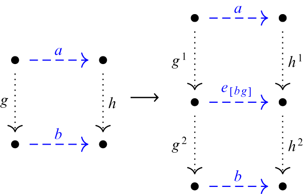
Figure 4: A commuting square in G and its “children” in
 $G_D$
, when
$G_D$
, when
 $h,g \in \mathcal {E}^{e_1}$
.
$h,g \in \mathcal {E}^{e_1}$
.
Case 1: Assume
 $\mu _1, \mu _2 \notin \bigcup _{i=1}^k \mathcal {E}_D^{e_i}$
. Then, we set
$\mu _1, \mu _2 \notin \bigcup _{i=1}^k \mathcal {E}_D^{e_i}$
. Then, we set
 $[\mu ]_D = \iota ^{-1}([\iota (\mu )])$
.
$[\mu ]_D = \iota ^{-1}([\iota (\mu )])$
.
Case 2: Suppose
 $\mu _j$
lies in
$\mu _j$
lies in
 $ \mathcal {E}^{e_1}_D$
, so that
$ \mathcal {E}^{e_1}_D$
, so that
 $\mu _j \in \{ g^1, g^2\}$
for some edge
$\mu _j \in \{ g^1, g^2\}$
for some edge
 $g \in \mathcal {E}^{e_1}$
. If
$g \in \mathcal {E}^{e_1}$
. If
 $j=1$
and
$j=1$
and
 $\mu _1 = g^2$
, then
$\mu _1 = g^2$
, then
 $r(\mu _1) = s(\mu _2) = \iota ^{-1}( r(g)) \in \iota ^{-1}(\Lambda ^0)$
, and the edges in
$r(\mu _1) = s(\mu _2) = \iota ^{-1}( r(g)) \in \iota ^{-1}(\Lambda ^0)$
, and the edges in
 $G_D$
with source in
$G_D$
with source in
 $\iota ^{-1}(\Lambda ^0)$
and degree
$\iota ^{-1}(\Lambda ^0)$
and degree
 $e_i$
for
$e_i$
for
 $i \not = 1$
are in
$i \not = 1$
are in
 $\iota ^{-1}(\Lambda ^1)$
. Therefore,
$\iota ^{-1}(\Lambda ^1)$
. Therefore,
 $\mu _2 \in \iota ^{-1}(\Lambda ^{e_i})$
, and
$\mu _2 \in \iota ^{-1}(\Lambda ^{e_i})$
, and
 $\iota (\mu _2) g$
is a bicolor path in G, so
$\iota (\mu _2) g$
is a bicolor path in G, so
 $\iota (\mu _2) g \sim h a$
for edges
$\iota (\mu _2) g \sim h a$
for edges
 $h \in \mathcal {E}^{e_1}, a \in \Lambda ^{e_i}$
. There is then an edge
$h \in \mathcal {E}^{e_1}, a \in \Lambda ^{e_i}$
. There is then an edge
 $e_{[\mu _2 g]} \in \Lambda ^{e_i}_D$
with source
$e_{[\mu _2 g]} \in \Lambda ^{e_i}_D$
with source
 $s(\mu _1) = v_g$
and range
$s(\mu _1) = v_g$
and range
 $v_h = s(h^2)$
; we define
$v_h = s(h^2)$
; we define
 $\mu _2 \mu _1 = \mu _2 g^2 \sim _D h^2 e_{[\mu _2 g]}$
. If
$\mu _2 \mu _1 = \mu _2 g^2 \sim _D h^2 e_{[\mu _2 g]}$
. If
 $j =1$
and
$j =1$
and
 $\mu _1 = g^1$
, the only edges in
$\mu _1 = g^1$
, the only edges in
 $G_D$
with source
$G_D$
with source
 $r(g^1) = v_g $
and degree
$r(g^1) = v_g $
and degree
 $e_i$
for
$e_i$
for
 $i \not =1$
are of the form
$i \not =1$
are of the form
 $e_{[bg ]} = e_{[ha]}$
for some commuting square
$e_{[bg ]} = e_{[ha]}$
for some commuting square
 $bg \sim ha $
in
$bg \sim ha $
in
 $ \Lambda $
. In this case, we will have
$ \Lambda $
. In this case, we will have
 $h \in \mathcal {E}^{e_1}$
, and
$h \in \mathcal {E}^{e_1}$
, and
 $r(h^1) = v_h = r(e_{[bg]})$
, so we set
$r(h^1) = v_h = r(e_{[bg]})$
, so we set
 $e_{[bg]} g^1 \sim _D h^1 a$
.
$e_{[bg]} g^1 \sim _D h^1 a$
.
A similar argument shows that if
 $j=2$
, the path
$j=2$
, the path
 $\mu _2 \mu _1$
will be of the form
$\mu _2 \mu _1$
will be of the form
 $h^1 a$
or
$h^1 a$
or
 $h^2 e_{[ha]}$
, whose factorizations we have already described.
$h^2 e_{[ha]}$
, whose factorizations we have already described.
Case 3: Assume
 $\mu $
is of the form
$\mu $
is of the form
 $e_{\beta } e_{\alpha }$
for
$e_{\beta } e_{\alpha }$
for
 $\alpha \in \mathcal {E}_D^{e_i}$
, and
$\alpha \in \mathcal {E}_D^{e_i}$
, and
 $\beta \in \mathcal {E}_D^{e_j}$
with
$\beta \in \mathcal {E}_D^{e_j}$
with
 $i \neq j$
. Now,
$i \neq j$
. Now,
 $s_D(e_{\beta }) = r_D(e_{\alpha }) = v_g$
for some
$s_D(e_{\beta }) = r_D(e_{\alpha }) = v_g$
for some
 $g \in \mathcal {E}^{e_1}$
, and consequently
$g \in \mathcal {E}^{e_1}$
, and consequently
 $\alpha , \beta \in \Lambda $
are linked as shown on the left-hand side of Figure 5. Because
$\alpha , \beta \in \Lambda $
are linked as shown on the left-hand side of Figure 5. Because
 $\Lambda $
is a k-graph, the 3-color path outlining
$\Lambda $
is a k-graph, the 3-color path outlining
 $\beta \alpha $
generates a 3-cube in
$\beta \alpha $
generates a 3-cube in
 $\Lambda $
, which is depicted on the right-hand side of Figure 5. Let
$\Lambda $
, which is depicted on the right-hand side of Figure 5. Let
 $\delta $
and
$\delta $
and
 $\gamma $
denote the faces of this cube which lie, respectively, opposite
$\gamma $
denote the faces of this cube which lie, respectively, opposite
 $\beta $
and
$\beta $
and
 $\alpha $
. Because
$\alpha $
. Because
 $g \in \mathcal {E}^{e_1}$
, all of the vertical edges of this cube are in
$g \in \mathcal {E}^{e_1}$
, all of the vertical edges of this cube are in
 $\mathcal {E}^{e_1},$
and so
$\mathcal {E}^{e_1},$
and so
 $\delta \in \mathcal {E}^{e_j}, \gamma \in \mathcal {E}^{e_i}.$
Moreover, the path
$\delta \in \mathcal {E}^{e_j}, \gamma \in \mathcal {E}^{e_i}.$
Moreover, the path
 $e_{\gamma } e_{\delta }$
is composable in
$e_{\gamma } e_{\delta }$
is composable in
 $\Lambda _D$
, and has the same source and range as
$\Lambda _D$
, and has the same source and range as
 $e_{\beta } e_{\alpha }$
. Set
$e_{\beta } e_{\alpha }$
. Set
 $e_{\beta } e_{\alpha } \sim _D e_{\gamma } e_{\delta }$
.
$e_{\beta } e_{\alpha } \sim _D e_{\gamma } e_{\delta }$
.
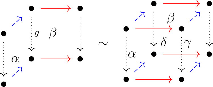
Figure 5: The commuting squares of edges from
 $ {\bigcup }_{i=2}^k {\mathcal {E}}_{D}^{e_i}$
.
$ {\bigcup }_{i=2}^k {\mathcal {E}}_{D}^{e_i}$
.
Observe that there are no two-color paths in
 $G_D^2$
of the form
$G_D^2$
of the form
 $g e_{\alpha }$
or
$g e_{\alpha }$
or
 $e_{\alpha } g$
for
$e_{\alpha } g$
for
 $g \in \iota ^{-1}(\Lambda ^1)$
and
$g \in \iota ^{-1}(\Lambda ^1)$
and
 $\alpha \in \mathcal {E}^{e_i}$
, because
$\alpha \in \mathcal {E}^{e_i}$
, because
 $ r_D(g) , s_D(g) \in \iota ^{-1}(\Lambda ^0)$
but
$ r_D(g) , s_D(g) \in \iota ^{-1}(\Lambda ^0)$
but
 $r_D(e_{\alpha }), s_D(e_{\alpha }) \in \{ v_e: e \in \mathcal {E}^{e_1}\}.$
Extend
 $\sim _D$
to be an equivalence relation on
$\sim _D$
to be an equivalence relation on
 $G^*_D$
which satisfies (KG0) and (KG1); observe that
$G^*_D$
which satisfies (KG0) and (KG1); observe that
 $\sim _D$
satisfies (KG2) by construction. Define
$\sim _D$
satisfies (KG2) by construction. Define
 $\Lambda _D = G_D^* / \sim _D$
. We call
$\Lambda _D = G_D^* / \sim _D$
. We call
 $\Lambda _D$
the graph of
$\Lambda _D$
the graph of
 $\Lambda $
delayed at the edge e.
$\Lambda $
delayed at the edge e.
Theorem 4.1 If
 $\Lambda $
is a row-finite source-free k-graph, then
$\Lambda $
is a row-finite source-free k-graph, then
 $\Lambda _D$
is also a row-finite source-free k-graph.
$\Lambda _D$
is also a row-finite source-free k-graph.
Proof Let
 $(\Lambda , d)$
be a k-graph, and let
$(\Lambda , d)$
be a k-graph, and let
 $(\Lambda _D, d_D)$
be the graph of
$(\Lambda _D, d_D)$
be the graph of
 $\Lambda $
delayed at the edge
$\Lambda $
delayed at the edge
 $e \in \Lambda ^{e_1}$
. Because
$e \in \Lambda ^{e_1}$
. Because
 $\sim _D$
satisfies (KG0), (KG1), and (KG2) by construction, it suffices to show that
$\sim _D$
satisfies (KG0), (KG1), and (KG2) by construction, it suffices to show that
 $\sim _D$
satisfies (KG3). Let
$\sim _D$
satisfies (KG3). Let
 $\mu = \mu _3 \mu _2 \mu _1 \in G_D^3$
be a tricolored path. Consider the following cases.
$\mu = \mu _3 \mu _2 \mu _1 \in G_D^3$
be a tricolored path. Consider the following cases.
Case 1: Assume
 $\mu _j \notin \bigcup \limits _{i=1}^k \mathcal {E}_D^{e_i}$
for all
$\mu _j \notin \bigcup \limits _{i=1}^k \mathcal {E}_D^{e_i}$
for all
 $j \in \{1,2,3\}$
. Then,
$j \in \{1,2,3\}$
. Then,
 $\iota (\mu )$
is a 3-colored path in
$\iota (\mu )$
is a 3-colored path in
 $\Lambda $
. Because we defined
$\Lambda $
. Because we defined
 $[\mu ]_D = \iota ^{-1}([\iota (\mu )])$
, the fact that
$[\mu ]_D = \iota ^{-1}([\iota (\mu )])$
, the fact that
 $\Lambda $
satisfies (KG3)—hence, that
$\Lambda $
satisfies (KG3)—hence, that
 $\iota (\mu )$
uniquely determines a 3-cube in
$\iota (\mu )$
uniquely determines a 3-cube in
 $\Lambda $
—implies that
$\Lambda $
—implies that
 $\mu $
also gives rise to a well-defined 3-cube in
$\mu $
also gives rise to a well-defined 3-cube in
 $\Lambda _D$
.
$\Lambda _D$
.
Case 2: Assume
 $\mu _j \in \mathcal {E}_D^{e_1}$
for one
$\mu _j \in \mathcal {E}_D^{e_1}$
for one
 $j \in \{ 1,2,3\}$
. Then,
$j \in \{ 1,2,3\}$
. Then,
 $\mu $
has one of the forms of tricolored paths on the right-hand side of Figure 6. This follows from Definition 4.0.1, specifically the restrictions for when an edge in
$\mu $
has one of the forms of tricolored paths on the right-hand side of Figure 6. This follows from Definition 4.0.1, specifically the restrictions for when an edge in
 $\iota ^{-1}(\Lambda ^1)$
can precede or follow an edge in
$\iota ^{-1}(\Lambda ^1)$
can precede or follow an edge in
 $\mathcal {E}_D^{e_1}$
, and when an edge in
$\mathcal {E}_D^{e_1}$
, and when an edge in
 $\mathcal {E}_D^{e_i}$
can precede or follow an edge in
$\mathcal {E}_D^{e_i}$
can precede or follow an edge in
 $\mathcal {E}_D^{e_1}$
.
$\mathcal {E}_D^{e_1}$
.
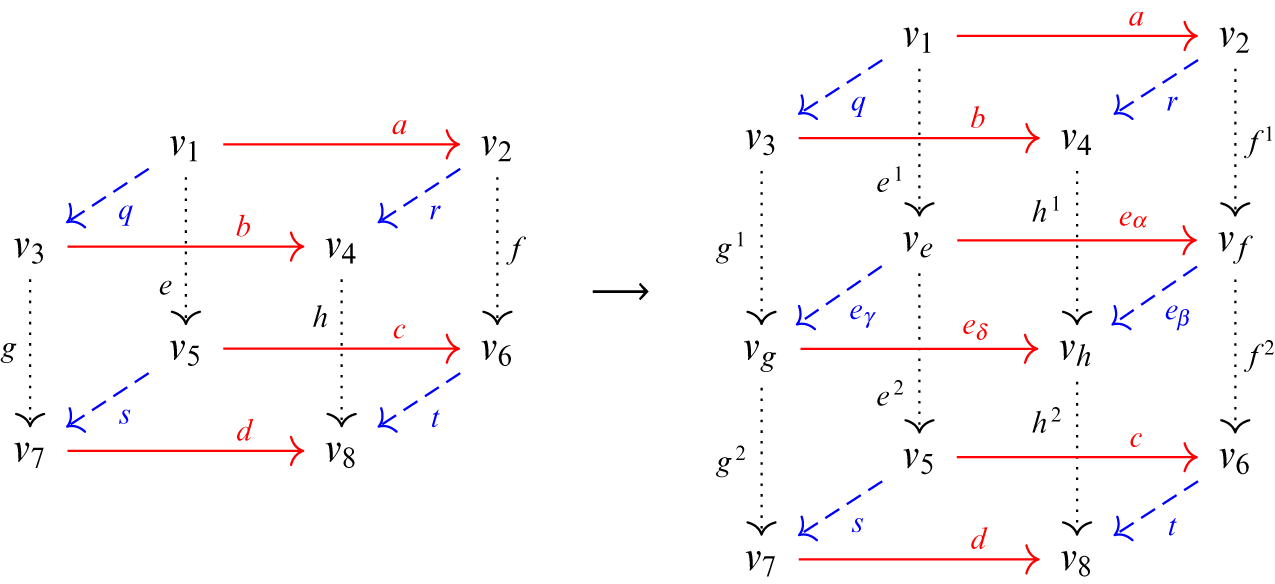
Figure 6: A commuting cube in G and its “children” in
 $G_D$
, when
$G_D$
, when
 $e,f,g,h \in \mathcal {E}_D^{e_1}$
.
$e,f,g,h \in \mathcal {E}_D^{e_1}$
.
For example, suppose
 $\mu _2 = g^2$
for some
$\mu _2 = g^2$
for some
 $g \in \mathcal E^{e_1}$
. Then,
$g \in \mathcal E^{e_1}$
. Then,
 $s_D(\mu _2) = r_D(\mu _1) = v_g$
, so
$s_D(\mu _2) = r_D(\mu _1) = v_g$
, so
 $\mu _1$
must be of the form
$\mu _1$
must be of the form
 $e_{\gamma }$
for some
$e_{\gamma }$
for some
 $\gamma \in \mathcal {E}^{e_i}$
with
$\gamma \in \mathcal {E}^{e_i}$
with
 $\gamma = [g q]$
. Then,
$\gamma = [g q]$
. Then,
 $r_D(\mu _2) = s_D(\mu _3) = \iota ^{-1}(r(g))$
, and because
$r_D(\mu _2) = s_D(\mu _3) = \iota ^{-1}(r(g))$
, and because
 $d(\mu _3) \not \in \{e_1, e_i\}$
, we must have
$d(\mu _3) \not \in \{e_1, e_i\}$
, we must have
 $\mu _3 \in \iota ^{-1}(\Lambda ^{e_j})$
for some
$\mu _3 \in \iota ^{-1}(\Lambda ^{e_j})$
for some
 $j \not = i$
. But then,
$j \not = i$
. But then,
 $\iota ^{-1}(\mu _3) g q \in G^3$
is a 3-color path, which defines a unique 3-cube in
$\iota ^{-1}(\mu _3) g q \in G^3$
is a 3-color path, which defines a unique 3-cube in
 $\Lambda $
(as depicted on the left-hand side of Figure 6). It is now straightforward to check that the two routes for factoring
$\Lambda $
(as depicted on the left-hand side of Figure 6). It is now straightforward to check that the two routes for factoring
 $\mu $
in
$\mu $
in
 $\Lambda _D$
(as in (KG3)) arise as “children” of this cube in
$\Lambda _D$
(as in (KG3)) arise as “children” of this cube in
 $G_D$
, so the fact that
$G_D$
, so the fact that
 $\Lambda $
is a k-graph implies that the two routes for factoring
$\Lambda $
is a k-graph implies that the two routes for factoring
 $\mu $
in
$\mu $
in
 $\Lambda _D$
lead to the same result. A similar analysis of the other possibilities for having one edge
$\Lambda _D$
lead to the same result. A similar analysis of the other possibilities for having one edge
 $\mu _j \in \mathcal {E}^{e_1}_D$
reveals that whenever this occurs, the factorization of
$\mu _j \in \mathcal {E}^{e_1}_D$
reveals that whenever this occurs, the factorization of
 $\mu $
in
$\mu $
in
 $\Lambda _D$
satisfies (KG3).
$\Lambda _D$
satisfies (KG3).
We now observe that if a tricolored path without an edge from
 $\mathcal {E}^{e_1}_D$
contains an edge from
$\mathcal {E}^{e_1}_D$
contains an edge from
 $\bigcup _{i=2}^k \mathcal {E}^{e_i}_D,$
it must consist entirely of edges in
$\bigcup _{i=2}^k \mathcal {E}^{e_i}_D,$
it must consist entirely of edges in
 $\bigcup _{i=2}^k \mathcal {E}^{e_i}_D$
. To see this, suppose that a tricolored path contains
$\bigcup _{i=2}^k \mathcal {E}^{e_i}_D$
. To see this, suppose that a tricolored path contains
 $e_\gamma $
for a commuting square
$e_\gamma $
for a commuting square
 $\gamma \in \Lambda $
, but that
$\gamma \in \Lambda $
, but that
 $\mu $
contains no edges in
$\mu $
contains no edges in
 $\mathcal {E}^{e_1}_D$
. Because
$\mathcal {E}^{e_1}_D$
. Because
 $s(\gamma ), r(\gamma ) \in \Lambda ^0_D \backslash \iota ^{-1}(\Lambda ^0)$
, the edge(s) preceding and following
$s(\gamma ), r(\gamma ) \in \Lambda ^0_D \backslash \iota ^{-1}(\Lambda ^0)$
, the edge(s) preceding and following
 $e_\gamma $
must be of the form
$e_\gamma $
must be of the form
 $e_\alpha $
for some
$e_\alpha $
for some
 $\alpha \in \mathcal {E}^{e_i}$
. Repeating the argument for
$\alpha \in \mathcal {E}^{e_i}$
. Repeating the argument for
 $e_\alpha $
if necessary shows that
$e_\alpha $
if necessary shows that
 $\mu $
consists entirely of edges in
$\mu $
consists entirely of edges in
 $\bigcup _{i=2}^k \mathcal {E}^{e_i}_D$
.
$\bigcup _{i=2}^k \mathcal {E}^{e_i}_D$
.
Thus, the only remaining case is the following case.
Case 3: Assume
 $\mu _j \in \bigcup \limits _{i=2}^k \mathcal {E}_D^{e_i}$
for all
$\mu _j \in \bigcup \limits _{i=2}^k \mathcal {E}_D^{e_i}$
for all
 $j \in \{ 1,2,3\}$
, and without loss of generality, assume
$j \in \{ 1,2,3\}$
, and without loss of generality, assume
 $\mu = e_\alpha e_\beta e_\gamma $
is a blue–red–green path. Because of the definition of
$\mu = e_\alpha e_\beta e_\gamma $
is a blue–red–green path. Because of the definition of
 $s_D, r_D$
for edges of the form
$s_D, r_D$
for edges of the form
 $e_\lambda $
in
$e_\lambda $
in
 $G_D^1$
,
$G_D^1$
,
 $\mu \in G_D^*$
arises from a sequence of commuting squares
$\mu \in G_D^*$
arises from a sequence of commuting squares
 $\alpha , \beta , \gamma $
in
$\alpha , \beta , \gamma $
in
 $\Lambda $
which share edges in
$\Lambda $
which share edges in
 $\mathcal {E}^{e_1}$
. Figure 7 depicts (from left to right) the squares
$\mathcal {E}^{e_1}$
. Figure 7 depicts (from left to right) the squares
 $\gamma , \beta , \alpha \in \Lambda $
. The color in each square
$\gamma , \beta , \alpha \in \Lambda $
. The color in each square
 $\lambda $
reflects the color of its horizontal edges, as these determine the degree of the edge
$\lambda $
reflects the color of its horizontal edges, as these determine the degree of the edge
 $e_\lambda \in G_D^1$
.
$e_\lambda \in G_D^1$
.
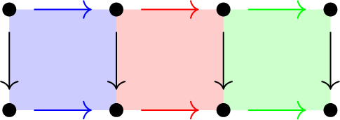
Figure 7: Factorization squares in
 $\Lambda $
that will be delayed to produce
$\Lambda $
that will be delayed to produce
 $\mu $
.
$\mu $
.
Because
 $\Lambda $
is a k-graph, the rectangle in Figure 7, which is reproduced in the top line of Figure 8, determines a unique four-dimensional cube in
$\Lambda $
is a k-graph, the rectangle in Figure 7, which is reproduced in the top line of Figure 8, determines a unique four-dimensional cube in
 $\Lambda $
. Thus, as we follow Route 1 of (KG3) and the instructions given in Case 3 of Definition 4.0.1 to factor
$\Lambda $
. Thus, as we follow Route 1 of (KG3) and the instructions given in Case 3 of Definition 4.0.1 to factor
 $$ \begin{align*}e_\alpha e_\beta e_\gamma = e_\alpha e_\eta e_\kappa = e_\delta e_\epsilon e_\kappa = e_\delta e_\phi e_\lambda,\end{align*} $$
the squares
 $\delta \phi \lambda $
—and indeed all of the intermediate squares—must lie on the four-dimensional cube determined by
$\delta \phi \lambda $
—and indeed all of the intermediate squares—must lie on the four-dimensional cube determined by
 $\alpha \beta \gamma $
. To be precise,
$\alpha \beta \gamma $
. To be precise,
 $\delta \phi \lambda $
is the collection of green–red–blue squares on the left-hand side of the bottom row of Figure 8. Similarly, when we factor
$\delta \phi \lambda $
is the collection of green–red–blue squares on the left-hand side of the bottom row of Figure 8. Similarly, when we factor
 $e_\alpha e_\beta e_\gamma $
via Route 2 of (KG3), we obtain the green–red–blue squares on the right-hand side of the bottom row of Figure 8. Because these squares lie on the same 4-cube as
$e_\alpha e_\beta e_\gamma $
via Route 2 of (KG3), we obtain the green–red–blue squares on the right-hand side of the bottom row of Figure 8. Because these squares lie on the same 4-cube as
 $\delta \phi \lambda $
, and in the same position (compare the position of
$\delta \phi \lambda $
, and in the same position (compare the position of
 $\nu _0$
on both), they must equal
$\nu _0$
on both), they must equal
 $\delta \phi \lambda $
. It follows that applying either Route 1 or Route 2 to
$\delta \phi \lambda $
. It follows that applying either Route 1 or Route 2 to
 $e_\alpha e_\beta e_\gamma $
gives us the same 3-colored path in
$e_\alpha e_\beta e_\gamma $
gives us the same 3-colored path in
 $G_D$
.
$G_D$
.
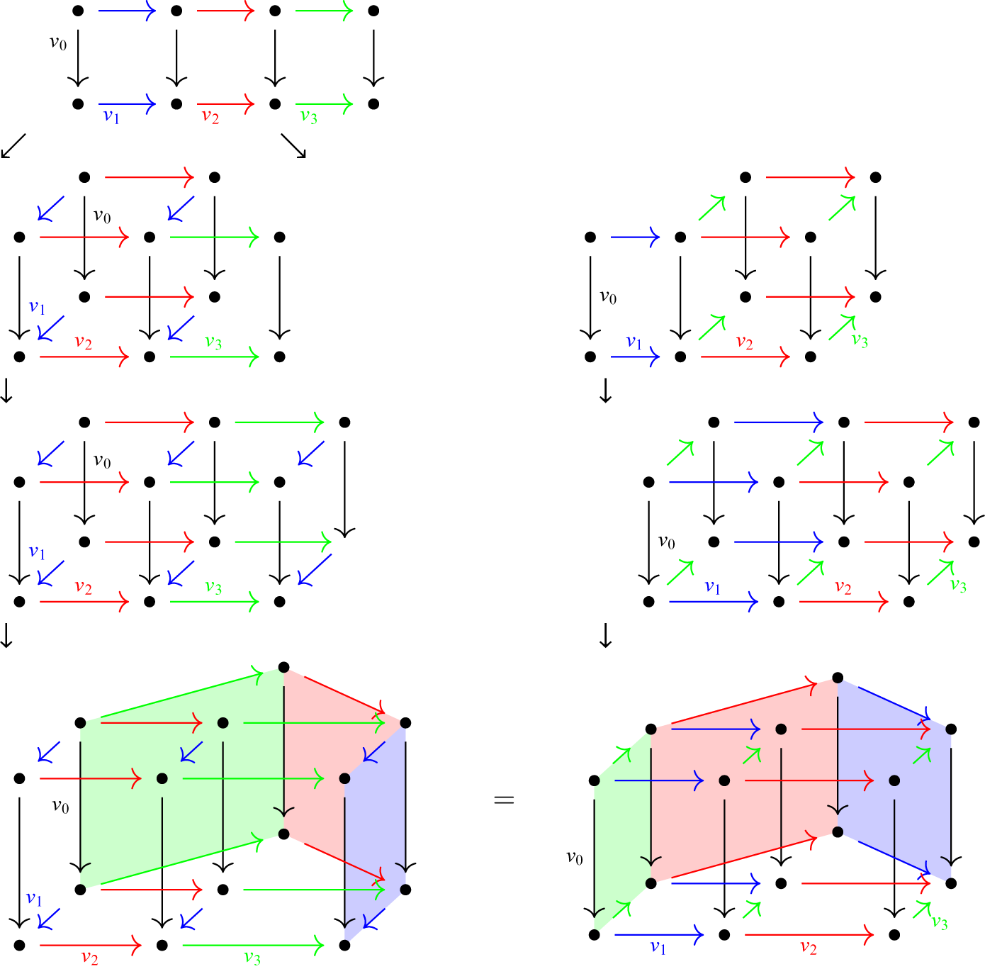
Figure 8: Associativity in
 $\Lambda _D$
via factorization squares in
$\Lambda _D$
via factorization squares in
 $\Lambda $
.
$\Lambda $
.
Having confirmed that the factorization of an arbitrary tricolored path in
 $G_D$
satisfies (KG3), we conclude that
$G_D$
satisfies (KG3), we conclude that
 $\Lambda _D$
is a k-graph.
$\Lambda _D$
is a k-graph.
It remains to check that
 $\Lambda _D$
is source-free and row-finite whenever
$\Lambda _D$
is source-free and row-finite whenever
 $\Lambda $
is. In constructing
$\Lambda $
is. In constructing
 $\Lambda _D$
, all newly created vertices
$\Lambda _D$
, all newly created vertices
 $v_g$
have an edge
$v_g$
have an edge
 $g^2$
of color 1 emanating from them. Moreover, because
$g^2$
of color 1 emanating from them. Moreover, because
 $r(g)$
is not a source in
$r(g)$
is not a source in
 $\Lambda $
, there is an edge
$\Lambda $
, there is an edge
 $b_i \in \Lambda ^{e_i} r(g)$
for each
$b_i \in \Lambda ^{e_i} r(g)$
for each
 $i \geq 2$
. Then,
$i \geq 2$
. Then,
 $[b_i g] \in \mathcal {E}^{e_i}$
and hence
$[b_i g] \in \mathcal {E}^{e_i}$
and hence
 $e_{[b_i g]}\in \Lambda ^{e_i}_D v_g$
for all
$e_{[b_i g]}\in \Lambda ^{e_i}_D v_g$
for all
 $i \geq 2$
. In other words, all of the new vertices
$i \geq 2$
. In other words, all of the new vertices
 $v_g$
emit at least one edge of each color.
$v_g$
emit at least one edge of each color.
Similarly, every vertex
 $v \in \iota ^{-1}(\Lambda ^0)$
emits an edge of each color, because the same is true in
$v \in \iota ^{-1}(\Lambda ^0)$
emits an edge of each color, because the same is true in
 $\Lambda $
; if v emits an edge
$\Lambda $
; if v emits an edge
 $ g \in \mathcal {E}^{e_1}$
then
$ g \in \mathcal {E}^{e_1}$
then
 $s_D(g^1) = \iota ^{-1}(s(g)) = v$
, and all other edges emitted by
$s_D(g^1) = \iota ^{-1}(s(g)) = v$
, and all other edges emitted by
 $\iota (v)$
are in
$\iota (v)$
are in
 $\iota (\Lambda _D^1)$
and hence also occur in
$\iota (\Lambda _D^1)$
and hence also occur in
 $\Lambda _D$
.
$\Lambda _D$
.
Furthermore, the number of edges with range v in
 $\Lambda _D$
is the same as the number of edges with range
$\Lambda _D$
is the same as the number of edges with range
 $\iota (v) \in \Lambda $
, if
$\iota (v) \in \Lambda $
, if
 $v \not = v_g$
. In this setting, an edge in
$v \not = v_g$
. In this setting, an edge in
 $v \Lambda _D^1 \backslash \iota ^{-1}(v\Lambda ^1_D)$
is necessarily of the form
$v \Lambda _D^1 \backslash \iota ^{-1}(v\Lambda ^1_D)$
is necessarily of the form
 $g^2$
for some
$g^2$
for some
 $g \in v\mathcal {E}^{e_1}$
, so
$g \in v\mathcal {E}^{e_1}$
, so
 $$ \begin{align*} | r_D^{-1}(v)| = |v\mathcal{E}^{e_1}| + |\iota^{-1}(v\Lambda^1_D)| = |r^{-1}(\iota(v))|.\end{align*} $$
If
 $v = v_g$
, then
$v = v_g$
, then
 $r_D^{-1}(v)$
is still finite as long as
$r_D^{-1}(v)$
is still finite as long as
 $\Lambda $
is row-finite:
$\Lambda $
is row-finite:
 $$ \begin{align*} |r_D^{-1}(v_g) | &= \left| \{ g^1\} \cup \bigcup_{i=2}^k v_g \mathcal{E}^{e_i}_D \right| \leq 1 + \left| \{ \alpha \in \Lambda: \alpha = [g b] \text{ for some } b \in \Lambda^1 \} \right| \\ &= 1 + r^{-1}(s(g)) < \infty. \end{align*} $$
We conclude that
 $\Lambda _D$
is a row-finite, source-free k-graph whenever
$\Lambda _D$
is a row-finite, source-free k-graph whenever
 $\Lambda $
is. ▪
$\Lambda $
is. ▪
Theorem 4.2 Let
 $(\Lambda , d)$
be a row-finite, source-free k-graph and let
$(\Lambda , d)$
be a row-finite, source-free k-graph and let
 $(\Lambda _D,d_D)$
be the graph of
$(\Lambda _D,d_D)$
be the graph of
 $\Lambda $
delayed at an edge f. Then,
$\Lambda $
delayed at an edge f. Then,
 $C^*(\Lambda _D)$
is Morita equivalent to
$C^*(\Lambda _D)$
is Morita equivalent to
 $C^*(\Lambda )$
.
$C^*(\Lambda )$
.
Proof Let
 $\{ t_\lambda : \lambda \in \Lambda _D^1 \cup \Lambda _D^0 \}$
be the canonical Cuntz–Krieger
$\{ t_\lambda : \lambda \in \Lambda _D^1 \cup \Lambda _D^0 \}$
be the canonical Cuntz–Krieger
 $\Lambda _{D}$
-family generating
$\Lambda _{D}$
-family generating
 $C^*(\Lambda _{D})$
. Define
$C^*(\Lambda _{D})$
. Define
 $$ \begin{align*} &S_{v} = t_{v}, \text{ for } v \in \Lambda^{0}, \\ &S_{h} = \left\{ \begin{array}{@{}ll} t_{\iota^{-1}(h)} & \text{if } h \notin \mathcal{E}^{e_{1}}\\ t_{h^{2}}t_{h^1} & \text{if } h \in \mathcal{E}^{e_{1}} \end{array} \right. \text{, for } h \in \Lambda^{1}. \end{align*} $$
We claim that
 $\{S_\lambda : \lambda \in \Lambda ^0 \cup \Lambda ^1 \}$
is a Cuntz–Krieger
$\{S_\lambda : \lambda \in \Lambda ^0 \cup \Lambda ^1 \}$
is a Cuntz–Krieger
 $\Lambda $
-family in
$\Lambda $
-family in
 $C^*(\Lambda _D)$
. Note that because
$C^*(\Lambda _D)$
. Note that because
 $\{t_v: v \in \Lambda ^0_D \}$
are mutually orthogonal projections, so are
$\{t_v: v \in \Lambda ^0_D \}$
are mutually orthogonal projections, so are
 $\{S_{v}: v \in \Lambda ^0 \}$
. Therefore,
$\{S_{v}: v \in \Lambda ^0 \}$
. Therefore,
 $\{S_\lambda : \lambda \in \Lambda ^0 \cup \Lambda ^1 \}$
satisfies (CK1). Now, take arbitrary
$\{S_\lambda : \lambda \in \Lambda ^0 \cup \Lambda ^1 \}$
satisfies (CK1). Now, take arbitrary
 $a,b,g,h \in \Lambda ^1$
such that
$a,b,g,h \in \Lambda ^1$
such that
 $ah \sim gb$
. Assuming
$ah \sim gb$
. Assuming
 $a,b,g,h \notin \mathcal {E}^{e_1}$
, Case 1 of Definition 4.0.1 implies that
$a,b,g,h \notin \mathcal {E}^{e_1}$
, Case 1 of Definition 4.0.1 implies that
 $$ \begin{align*} S_a S_h = t_{\iota^{-1}(a)} t_{\iota^{-1}(h)} = t_{\iota^{-1}(g)} t_{\iota^{-1}(b)} = S_g S_b. \end{align*} $$
Conversely, suppose either
 $a,b \in \mathcal {E}^{e_1}$
, or
$a,b \in \mathcal {E}^{e_1}$
, or
 $g,h \in \mathcal {E}^{e_1}$
. Without loss of generality, assume
$g,h \in \mathcal {E}^{e_1}$
. Without loss of generality, assume
 $g,h \in \mathcal {E}^{e_1}$
. Then,
$g,h \in \mathcal {E}^{e_1}$
. Then,
 $\alpha := [ah] \in \mathcal {E}_{D}^{e_{i}}$
satisfies
$\alpha := [ah] \in \mathcal {E}_{D}^{e_{i}}$
satisfies
 $e_{\alpha } h^1 \sim _D g^1 b$
and
$e_{\alpha } h^1 \sim _D g^1 b$
and
 $a h^2 \sim _D g^2 e_\alpha $
. Hence,
$a h^2 \sim _D g^2 e_\alpha $
. Hence,
 $$ \begin{align*} S_a S_h = t_a t_{h^2} t_{h^1} = t_{g^2} t_{e_{\alpha}} t_{h^1} = t_{g^2} t_{g^1} t_b = S_gS_b. \end{align*} $$
Therefore,
 $\{S_\lambda : \lambda \in \Lambda ^0 \cup \Lambda ^1 \}$
satisfies (CK2).
$\{S_\lambda : \lambda \in \Lambda ^0 \cup \Lambda ^1 \}$
satisfies (CK2).
For (CK3), let
 $h \in \Lambda ^1 \setminus \mathcal {E}^{e_{1}}$
; observe that
$h \in \Lambda ^1 \setminus \mathcal {E}^{e_{1}}$
; observe that
 $S_{h} = t_{h}$
, and hence
$S_{h} = t_{h}$
, and hence
 $ S_h^* S_h = t_h^* t_h = t_{s_D(h)} = S_{s(h)}.$
If
$ S_h^* S_h = t_h^* t_h = t_{s_D(h)} = S_{s(h)}.$
If
 $h \in \mathcal {E}^{e_{1}}$
, we similarly have
$h \in \mathcal {E}^{e_{1}}$
, we similarly have
 $ S_h^* S_h = t_{h^1}^* t_{h^2}^* t_{h^2} t_{h^1} = t_{s_D(h)} = S_{s(h)}.$
Therefore,
$ S_h^* S_h = t_{h^1}^* t_{h^2}^* t_{h^2} t_{h^1} = t_{s_D(h)} = S_{s(h)}.$
Therefore,
 $\{S_\lambda : \lambda \in \Lambda ^0 \cup \Lambda ^1 \}$
satisfies (CK3).
$\{S_\lambda : \lambda \in \Lambda ^0 \cup \Lambda ^1 \}$
satisfies (CK3).
Finally, take an arbitrary
 $v \in \Lambda ^0$
. Observe that if
$v \in \Lambda ^0$
. Observe that if
 $h \in \mathcal {E}^{e_1}$
, then
$h \in \mathcal {E}^{e_1}$
, then
 $h^1$
is the only edge in
$h^1$
is the only edge in
 $\Lambda _D$
such that
$\Lambda _D$
such that
 $d_D(h_1) = e_1$
and
$d_D(h_1) = e_1$
and
 $r_D(h_1) = v_h$
. Thus,
$r_D(h_1) = v_h$
. Thus,
 $t_{v_h} = t_{h^1} t_{h^1}^*$
and consequently
$t_{v_h} = t_{h^1} t_{h^1}^*$
and consequently
 $$ \begin{align*} \sum_{h \in r^{-1}(v) \cap \Lambda^{e_1}} S_h S_h^* &= \sum_{\substack{h \in r^{-1}(v) \cap \Lambda^{e_1} \\ h \notin \mathcal{E}^{e_1}}} t_{\iota^{-1}(h)} t_{\iota^{-1}(h)}^* + \sum_{\substack{h \in r^{-1}(v) \cap \Lambda^{e_1} \\ h \in \mathcal{E}^{e_1}}} t_{h^2} t_{h^1} t_{h^1}^* t_{h^2}^* \\ &= \sum_{\substack{h \in r^{-1}(v) \cap \Lambda^{e_{1}} \\ h \notin \mathcal{E}^{e_1}}} t_{\iota^{-1}(h)} t_{\iota^{-1}(h)}^* + \sum_{\substack{h \in r^{-1}(v) \cap \Lambda^{e_{1}} \\ h \in \mathcal{E}^{e_1}}} t_{h^2} t_{h^2}^* \\ &= \sum_{e \in r^{-1}_D(v) \cap \Lambda^{e_{1}}_D}t_{e}t_{e}^* = t_{v} = S_{v}. \end{align*} $$
Now, if
 $2 \leq i \leq k$
, the fact that
$2 \leq i \leq k$
, the fact that
 $v \in \Lambda ^0$
means that
$v \in \Lambda ^0$
means that
 $\iota ^{-1}(v) \Lambda ^{e_i}_D = \iota ^{-1}(v \Lambda ^{e_i})$
: there are no edges of the form
$\iota ^{-1}(v) \Lambda ^{e_i}_D = \iota ^{-1}(v \Lambda ^{e_i})$
: there are no edges of the form
 $h^j$
or
$h^j$
or
 $e_\alpha $
with range v and degree
$e_\alpha $
with range v and degree
 $e_i$
. Consequently,
$e_i$
. Consequently,
 $$ \begin{align*} \sum_{h \in \Lambda^{e_{i}}} S_{h}S_{h}^* = \sum_{h \in v\Lambda^{e_{i}}} t_{h}t_{h}^* = t_{v} = S_{v}. \end{align*} $$
Therefore,
 $\{S_\lambda : \lambda \in \Lambda ^0 \cup \Lambda ^1 \}$
satisfies (CK4), and hence is a Cuntz–Krieger
$\{S_\lambda : \lambda \in \Lambda ^0 \cup \Lambda ^1 \}$
satisfies (CK4), and hence is a Cuntz–Krieger
 $\Lambda $
-family in
$\Lambda $
-family in
 $C^*(\Lambda _{D})$
. By the universal property of
$C^*(\Lambda _{D})$
. By the universal property of
 $C^*(\Lambda )$
, there exists a homomorphism
$C^*(\Lambda )$
, there exists a homomorphism
 $\pi :C^*(\Lambda ) \rightarrow C^*(\Lambda _D)$
.
$\pi :C^*(\Lambda ) \rightarrow C^*(\Lambda _D)$
.
To see that that
 $\pi $
is injective, we use Theorem 2.4 and Lemma 2.5. Define
$\pi $
is injective, we use Theorem 2.4 and Lemma 2.5. Define
 $\beta : \mathbb {T}^{k} \to \text {Aut}(C^*(\Lambda _D))$
by setting, for all
$\beta : \mathbb {T}^{k} \to \text {Aut}(C^*(\Lambda _D))$
by setting, for all
 $z \in {\mathbb T}^k$
,
$z \in {\mathbb T}^k$
,
 $$ \begin{align*} &\beta_z(t_h) = z^{d(h)} t_h \text{, for } h \neq g^1, \\ &\beta_z(t_h) = t_h \text{, for } h = g^1, \\ &\beta_z(t_v) = t_v \text{, for } v \in \Lambda^0, \end{align*} $$
and extending
 $\beta $
to be linear and multiplicative. By applying Lemma 2.5, we see that
$\beta $
to be linear and multiplicative. By applying Lemma 2.5, we see that
 $\beta $
is an action of
$\beta $
is an action of
 $\mathbb {T}^k$
on
$\mathbb {T}^k$
on
 $C^*(\Lambda _D)$
. Let
$C^*(\Lambda _D)$
. Let
 $\alpha $
be the canonical gauge action on
$\alpha $
be the canonical gauge action on
 $C^*(\Lambda ) = C^*(\{ s_\lambda : \lambda \in \Lambda ^0 \cup \Lambda ^1\})$
and note that for
$C^*(\Lambda ) = C^*(\{ s_\lambda : \lambda \in \Lambda ^0 \cup \Lambda ^1\})$
and note that for
 $e \notin \mathcal {E}^{e_1}$
, we have
$e \notin \mathcal {E}^{e_1}$
, we have
 $$ \begin{align*} \pi[\alpha_z(s_{e})]= \pi[z^{d(e)}s_{e}] = z^{d(e)}S_{e} = z^{d(e)}t_{e} = \beta_z(t_{e})= \beta_z(T_{e}) = \beta_z(\pi[s_{e}]) \end{align*} $$
and for
 $e \in \mathcal {E}^{e_1}$
,
$e \in \mathcal {E}^{e_1}$
,
 $$ \begin{align*} \pi[\alpha_z(s_{e})] = \pi[z^{d(e)}s_{e}] = z^{d(e)}S_{e} = z^{d(e)}t_{e^2}t_{e^1} = \beta_z(t_{e^2}t_{e^1}) = \beta_z(T_{e}) = \beta_z(\pi[s_{e}]). \end{align*} $$
It is straightforward to check that
 $\alpha $
and
$\alpha $
and
 $\beta $
commute on the vertex projections. Therefore,
$\beta $
commute on the vertex projections. Therefore,
 $\beta $
commutes with the canonical gauge action, so Theorem 2.4 implies that
$\beta $
commutes with the canonical gauge action, so Theorem 2.4 implies that
 $\pi $
is injective.
$\pi $
is injective.
To see that
 $\text {Im}(\pi ) \cong C^*(\Lambda )$
is Morita equivalent to
$\text {Im}(\pi ) \cong C^*(\Lambda )$
is Morita equivalent to
 $C^*(\Lambda _D)$
, we invoke Theorem 2.6. Set
$C^*(\Lambda _D)$
, we invoke Theorem 2.6. Set
 $X = \iota ^{-1}(\Lambda ^0) \subseteq \Lambda ^0_D$
; we will show that the saturation
$X = \iota ^{-1}(\Lambda ^0) \subseteq \Lambda ^0_D$
; we will show that the saturation
 $\Sigma (X)$
of X is
$\Sigma (X)$
of X is
 $\Lambda ^0_D$
. If
$\Lambda ^0_D$
. If
 $g \in \mathcal {E}^{e_1}$
, then
$g \in \mathcal {E}^{e_1}$
, then
 $r(g) \in \iota (\Lambda _D^0)$
and
$r(g) \in \iota (\Lambda _D^0)$
and
 $g^2 \in \iota ^{-1}(r(g)) \Lambda _D$
. Therefore, if H is hereditary and contains X, we must have
$g^2 \in \iota ^{-1}(r(g)) \Lambda _D$
. Therefore, if H is hereditary and contains X, we must have
 $s_D(g^2) = v_g \in H$
for all
$s_D(g^2) = v_g \in H$
for all
 $g \in \mathcal {E}^{e_1}$
. Consequently,
$g \in \mathcal {E}^{e_1}$
. Consequently,
 $H = \Lambda _D^0$
. Because
$H = \Lambda _D^0$
. Because
 $\Lambda ^0_D$
is evidently saturated, we have
$\Lambda ^0_D$
is evidently saturated, we have
 $\Sigma (X) = \Lambda ^0_D$
as claimed. Theorem 2.6 therefore implies that
$\Sigma (X) = \Lambda ^0_D$
as claimed. Theorem 2.6 therefore implies that
 $$ \begin{align*} P_X C^*(\Lambda_D) P_X \cong_{ME} C^*(\Lambda_D).\end{align*} $$
We will now complete the proof that
 $C^*(\Lambda ) \cong _{ME} C^*(\Lambda _D)$
by showing that
$C^*(\Lambda ) \cong _{ME} C^*(\Lambda _D)$
by showing that
 $$ \begin{align*} P_X C^*(\Lambda_D) P_X = \text{Im}(\pi)\cong C^*(\Lambda).\end{align*} $$
The generators
 $\{ S_\lambda : \lambda \in \Lambda ^0 \cup \Lambda ^1\}$
of
$\{ S_\lambda : \lambda \in \Lambda ^0 \cup \Lambda ^1\}$
of
 $\text {Im}(\pi )$
all satisfy
$\text {Im}(\pi )$
all satisfy
 $P_X S_h P_X = S_h$
, so
$P_X S_h P_X = S_h$
, so
 $\text {Im}(\pi ) \subseteq P_X C^*(\Lambda _D) P_X$
. For the other inclusion, note that
$\text {Im}(\pi ) \subseteq P_X C^*(\Lambda _D) P_X$
. For the other inclusion, note that
 $$ \begin{align*} P_X C^*(\Lambda_D) P_X = \overline{\text{span}}\, \{ t_\lambda t_\mu^*: \lambda, \mu \in G_D^*,\ s_D(\lambda) = s_D(\mu) ,\ r(\lambda), r(\mu) \in X\}.\end{align*} $$
Given
 $\lambda \in G_D^*$
with
$\lambda \in G_D^*$
with
 $r_D(\lambda ) \in X$
, create
$r_D(\lambda ) \in X$
, create
 $\lambda ' \in [\lambda ]_D$
by first replacing any path of the form
$\lambda ' \in [\lambda ]_D$
by first replacing any path of the form
 $g^2 e_{[ah]}$
in
$g^2 e_{[ah]}$
in
 $\lambda $
with its equivalent
$\lambda $
with its equivalent
 $a h^2$
, and then replacing paths of the form
$a h^2$
, and then replacing paths of the form
 $e_{[gb]} h^1$
with their equivalent
$e_{[gb]} h^1$
with their equivalent
 $g^1 b$
. Note that because
$g^1 b$
. Note that because
 $r(\lambda ) = r_D(\lambda ) \in X$
, we cannot have
$r(\lambda ) = r_D(\lambda ) \in X$
, we cannot have
 $\lambda _{|\lambda |} \in \mathcal {E}^{e_i}_D$
for any
$\lambda _{|\lambda |} \in \mathcal {E}^{e_i}_D$
for any
 $i\not = 1.$
Because of this,
$i\not = 1.$
Because of this,
 $\lambda '$
will contain no edges in
$\lambda '$
will contain no edges in
 $\bigcup _{i=2}^k \mathcal {E}^{e_i}_D$
.
$\bigcup _{i=2}^k \mathcal {E}^{e_i}_D$
.
Thus, in
 $\lambda '$
, any occurrence of an edge of the form
$\lambda '$
, any occurrence of an edge of the form
 $g^2$
will be preceded by
$g^2$
will be preceded by
 $g^1$
unless
$g^1$
unless
 $s_D(\lambda ') \not \in X$
(in which case, if
$s_D(\lambda ') \not \in X$
(in which case, if
 $s_D(\lambda ^{\prime }) = v_g, \ \lambda ^{\prime }_1 = g^2$
). Consequently, if
$s_D(\lambda ^{\prime }) = v_g, \ \lambda ^{\prime }_1 = g^2$
). Consequently, if
 $s_D(\lambda ^{\prime }) \in X$
, then
$s_D(\lambda ^{\prime }) \in X$
, then
 $ t_{\lambda ^{\prime }_{|\lambda |}} \cdots t_{\lambda ^{\prime }_2} t_{\lambda ^{\prime }_1} = t_{\lambda ^{\prime }} = t_{\lambda }$
is a product of operators of the form
$ t_{\lambda ^{\prime }_{|\lambda |}} \cdots t_{\lambda ^{\prime }_2} t_{\lambda ^{\prime }_1} = t_{\lambda ^{\prime }} = t_{\lambda }$
is a product of operators of the form
 $S_h, S_k^*$
for
$S_h, S_k^*$
for
 $h, k \in \Lambda ^1$
.
$h, k \in \Lambda ^1$
.
Similarly, given
 $\mu \in G^*_D$
with
$\mu \in G^*_D$
with
 $r_D(\mu ) \in X$
and
$r_D(\mu ) \in X$
and
 $s_D(\mu ) = s_D(\lambda )$
, create
$s_D(\mu ) = s_D(\lambda )$
, create
 $\mu ^{\prime } \in [\mu ]_D$
by the procedure above, so that
$\mu ^{\prime } \in [\mu ]_D$
by the procedure above, so that
 $\mu ^{\prime }$
contains no edges in
$\mu ^{\prime }$
contains no edges in
 $\bigcup _{i=2}^k \mathcal {E}^{e_i}_D$
and any edge in
$\bigcup _{i=2}^k \mathcal {E}^{e_i}_D$
and any edge in
 $\mu ^{\prime }$
of the form
$\mu ^{\prime }$
of the form
 $g^2$
(with the possible exception of
$g^2$
(with the possible exception of
 $\mu ^{\prime }_1$
) is preceded by
$\mu ^{\prime }_1$
) is preceded by
 $g^1$
. It follows that for any
$g^1$
. It follows that for any
 $\mu , \lambda $
with
$\mu , \lambda $
with
 $r_D(\mu ), r_D(\lambda ) \in X$
and
$r_D(\mu ), r_D(\lambda ) \in X$
and
 $s_D(\mu ) = s_D(\lambda ) \in X$
, we have
$s_D(\mu ) = s_D(\lambda ) \in X$
, we have
 $t_\lambda t_\mu ^* \in \text {Im}(\pi )$
.
$t_\lambda t_\mu ^* \in \text {Im}(\pi )$
.
If
 $t_\lambda t_\mu ^* \in P_X C^*(\Lambda _D) P_X$
and
$t_\lambda t_\mu ^* \in P_X C^*(\Lambda _D) P_X$
and
 $s_D(\lambda )\not \in X$
, write
$s_D(\lambda )\not \in X$
, write
 $v_g = s_D(\lambda )$
. As observed earlier, in this case, we must have
$v_g = s_D(\lambda )$
. As observed earlier, in this case, we must have
 $\lambda ^{\prime }_1 = \mu ^{\prime }_1 = g^2.$
Moreover, because
$\lambda ^{\prime }_1 = \mu ^{\prime }_1 = g^2.$
Moreover, because
 $v_g$
receives precisely one edge of degree
$v_g$
receives precisely one edge of degree
 $e_1$
(namely
$e_1$
(namely
 $g^1$
), we have
$g^1$
), we have
 $p_{v_g} = t_{g^1} t_{g^1}^*$
. It follows that
$p_{v_g} = t_{g^1} t_{g^1}^*$
. It follows that
 $$ \begin{align*} t_\lambda t_\mu^* = t_{\lambda^{\prime}} t_{\mu^{\prime}}^* = t_{\lambda^{\prime} g^1} t_{\mu^{\prime} g^1}^*.\end{align*} $$
Observe that neither
 $\lambda ^{\prime } g^1$
nor
$\lambda ^{\prime } g^1$
nor
 $\mu ^{\prime } g^1$
contains any edge in
$\mu ^{\prime } g^1$
contains any edge in
 $\bigcup _{i=2}^k \mathcal {E}^{e_i}_D$
, and every occurrence of an edge of the form
$\bigcup _{i=2}^k \mathcal {E}^{e_i}_D$
, and every occurrence of an edge of the form
 $h^2$
in either path is preceded by
$h^2$
in either path is preceded by
 $h^1$
. Thus, in this case as well, we can write
$h^1$
. Thus, in this case as well, we can write
 $t_\lambda t_\mu ^*$
as a product of operators of the form
$t_\lambda t_\mu ^*$
as a product of operators of the form
 $S_h, S_k^*$
.
$S_h, S_k^*$
.
Because
 $\text {Im}(\pi )$
is norm-closed, it follows that every element in
$\text {Im}(\pi )$
is norm-closed, it follows that every element in
 $\overline {\text {span}} \{ t_\mu t_\lambda ^*: \lambda , \mu \in \Lambda _D, r(\lambda ) = r(\mu ) \in X \} = P_X C^*(\Lambda _D)P_X$
lies in
$\overline {\text {span}} \{ t_\mu t_\lambda ^*: \lambda , \mu \in \Lambda _D, r(\lambda ) = r(\mu ) \in X \} = P_X C^*(\Lambda _D)P_X$
lies in
 $\text {Im}(\pi )$
. Thus,
$\text {Im}(\pi )$
. Thus,
 $$ \begin{align*}C^*(\Lambda) \cong \text{Im}(\pi) = P_X C^*(\Lambda_D) P_X \cong_{ME} C^*(\Lambda_D),\end{align*} $$
as claimed. ▪
5 Sink deletion
In this section, we analyze the effect on
 $C^*(\Lambda )$
of deleting a sink—a vertex which emits no edges of a certain color—from
$C^*(\Lambda )$
of deleting a sink—a vertex which emits no edges of a certain color—from
 $\Lambda $
. This should be viewed as the analog of move (S), removing a regular source, for directed graphs, as the conventions used to define a Cuntz–Krieger family in [Reference Eilers, Restorff, Ruiz and SørensenERRS16, Reference SørensenSø13] differ from the standard conventions for higher-rank graph
$\Lambda $
. This should be viewed as the analog of move (S), removing a regular source, for directed graphs, as the conventions used to define a Cuntz–Krieger family in [Reference Eilers, Restorff, Ruiz and SørensenERRS16, Reference SørensenSø13] differ from the standard conventions for higher-rank graph
 $C^*$
-algebras. We show in Theorem 5.4 that the result of deleting a sink from a k-graph is still a k-graph, and Theorem 5.5 shows that the resulting
$C^*$
-algebras. We show in Theorem 5.4 that the result of deleting a sink from a k-graph is still a k-graph, and Theorem 5.5 shows that the resulting
 $C^*$
-algebra is Morita equivalent to the original k-graph
$C^*$
-algebra is Morita equivalent to the original k-graph
 $C^*$
-algebra.
$C^*$
-algebra.
Definition 5.0.1 Let
 $\Lambda $
be a k-graph. We say
$\Lambda $
be a k-graph. We say
 $v \in \Lambda ^0$
is an
$v \in \Lambda ^0$
is an
 $e_i$
sink if
$e_i$
sink if
 $s^{-1}(v) \cap \Lambda ^{e_i} = \emptyset $
for some
$s^{-1}(v) \cap \Lambda ^{e_i} = \emptyset $
for some
 $1 \leq i \leq k$
. We say v is a sink if it is an
$1 \leq i \leq k$
. We say v is a sink if it is an
 $e_i$
sink for some
$e_i$
sink for some
 $1 \leq i \leq k$
.
$1 \leq i \leq k$
.
Definition 5.0.2 Let
 $(\Lambda , d)$
be a k-graph. Let
$(\Lambda , d)$
be a k-graph. Let
 $G = (\Lambda ^0, \Lambda ^1, r, s)$
, and
$G = (\Lambda ^0, \Lambda ^1, r, s)$
, and
 $G^*$
be its 1-skeleton and category of paths, respectively. Let
$G^*$
be its 1-skeleton and category of paths, respectively. Let
 $v \in \Lambda ^0$
be a sink. We write
$v \in \Lambda ^0$
be a sink. We write
 $w \leq v$
if there exists a
$w \leq v$
if there exists a
 $\lambda \in G^*$
such that
$\lambda \in G^*$
such that
 $s(\lambda ) = v$
and
$s(\lambda ) = v$
and
 $r(\lambda ) = w$
. Define the directed colored graph
$r(\lambda ) = w$
. Define the directed colored graph
 $G_S = (\Lambda ^0_S, \Lambda ^1_S, r_S, s_S)$
by
$G_S = (\Lambda ^0_S, \Lambda ^1_S, r_S, s_S)$
by
 $$ \begin{align*} & \Lambda^0_S := \{ w: w \not\leq v\}, \qquad \Lambda^1_S : = \Lambda^1 \setminus \{ f \in \Lambda^1: r(f) \leq v \}; \end{align*} $$
we set
 $r_S = r, s_S = s,$
and
$r_S = r, s_S = s,$
and
 $d_S = d$
. Let
$d_S = d$
. Let
 $\iota : G^*_S \to G^*$
be the inclusion map, and define an equivalence relation on
$\iota : G^*_S \to G^*$
be the inclusion map, and define an equivalence relation on
 $G_S^*$
by
$G_S^*$
by
 $\mu \sim \lambda $
when
$\mu \sim \lambda $
when
 $[\iota (\mu )] = [\iota (\lambda )] \in \Lambda $
. Define
$[\iota (\mu )] = [\iota (\lambda )] \in \Lambda $
. Define
 $\Lambda _S = G^* / \sim $
and call
$\Lambda _S = G^* / \sim $
and call
 $\Lambda _S$
the k-graph of
$\Lambda _S$
the k-graph of
 $\Lambda $
with the sink v deleted.
$\Lambda $
with the sink v deleted.
Example 5.1 Consider the graph G below. The graph
 $G_S$
is the result of deleting the blue sink
$G_S$
is the result of deleting the blue sink
 $v$
of
$v$
of
 $G$
, where blue is the dashed color.
$G$
, where blue is the dashed color.
Example 5.2 The following example highlights the fact that performing a sink-deletion (Figure 9) may introduce new sinks. When
 $\Lambda $
has a finite vertex set, performing successive sink deletions will eventually produce a sink-free k-graph.
$\Lambda $
has a finite vertex set, performing successive sink deletions will eventually produce a sink-free k-graph.

Figure 9: Sink deletion at v creating a new sink at w.
Lemma 5.3 If
 $(\Lambda , d)$
is a k-graph with
$(\Lambda , d)$
is a k-graph with
 $v \in \Lambda ^0$
an
$v \in \Lambda ^0$
an
 $e_i$
sink, then
$e_i$
sink, then
 $ \{ x \in \Lambda ^0: x \leq v \}$
consists of
$ \{ x \in \Lambda ^0: x \leq v \}$
consists of
 $e_i$
sinks.
$e_i$
sinks.
Proof If
 $w \leq v $
and w is not an
$w \leq v $
and w is not an
 $e_i$
sink, then there exists a
$e_i$
sink, then there exists a
 $y \in \Lambda ^0$
and
$y \in \Lambda ^0$
and
 $f \in \Lambda ^{e_i}$
such that
$f \in \Lambda ^{e_i}$
such that
 $s(f) = w$
and
$s(f) = w$
and
 $r(f) = y$
. Thus, there exists a path
$r(f) = y$
. Thus, there exists a path
 $f \lambda \in s^{-1}(v) \cap r^{-1}(y).$
Furthermore, because
$f \lambda \in s^{-1}(v) \cap r^{-1}(y).$
Furthermore, because
 $\Lambda $
is a k-graph, there exists a path
$\Lambda $
is a k-graph, there exists a path
 $\mu g \sim f \lambda $
with
$\mu g \sim f \lambda $
with
 $g \in \Lambda ^{e_i}$
. That is, v is not an
$g \in \Lambda ^{e_i}$
. That is, v is not an
 $e_i$
sink. ▪
$e_i$
sink. ▪
Theorem 5.4 If
 $(\Lambda , d)$
is a source-free k-graph with
$(\Lambda , d)$
is a source-free k-graph with
 $v \in \Lambda ^0$
a sink, then
$v \in \Lambda ^0$
a sink, then
 $(\Lambda _S, d_S)$
, the graph of
$(\Lambda _S, d_S)$
, the graph of
 $\Lambda $
with the sink
$\Lambda $
with the sink
 $v \in \Lambda ^0$
deleted, is a source-free k-graph.
$v \in \Lambda ^0$
deleted, is a source-free k-graph.
Proof Take
 $\lambda \in G_S^*$
. Because
$\lambda \in G_S^*$
. Because
 $r(\iota (\lambda )) \not \leq v$
, if
$r(\iota (\lambda )) \not \leq v$
, if
 $\mu = \mu _1 \cdots \mu _n \sim \iota (\lambda )$
, then
$\mu = \mu _1 \cdots \mu _n \sim \iota (\lambda )$
, then
 $r(\mu ) \not \leq v$
. In fact, we have
$r(\mu ) \not \leq v$
. In fact, we have
 $s(\mu ) = s(\iota (\lambda )) \not \leq v$
, and
$s(\mu ) = s(\iota (\lambda )) \not \leq v$
, and
 $r(\mu _i) \notin V$
for all
$r(\mu _i) \notin V$
for all
 $1 \leq i \leq n$
. To see this, simply recall that if
$1 \leq i \leq n$
. To see this, simply recall that if
 $s(\eta ) \leq v$
, then
$s(\eta ) \leq v$
, then
 $r(\eta ) \leq v$
as well. Consequently,
$r(\eta ) \leq v$
as well. Consequently,
 $\mu \in \iota (G_S^*)$
and
$\mu \in \iota (G_S^*)$
and
 $\iota ^{-1}(\mu ) \sim _S \lambda $
. Thus,
$\iota ^{-1}(\mu ) \sim _S \lambda $
. Thus,
 $[\lambda ]_S = [\iota (\lambda )]$
, which satisfies (KG0) and (KG4), because
$[\lambda ]_S = [\iota (\lambda )]$
, which satisfies (KG0) and (KG4), because
 $\Lambda $
is a k-graph. Because
$\Lambda $
is a k-graph. Because
 $\lambda \in G_S^*$
was arbitrary, it follows that
$\lambda \in G_S^*$
was arbitrary, it follows that
 $\Lambda _S$
is a k-graph.
$\Lambda _S$
is a k-graph.
To see that
 $\Lambda _S$
is source-free, note that whenever an edge
$\Lambda _S$
is source-free, note that whenever an edge
 $e \in G^1$
was deleted in the process of forming
$e \in G^1$
was deleted in the process of forming
 $\Lambda _S$
, so too was the vertex
$\Lambda _S$
, so too was the vertex
 $r(e) \in G^0$
. Therefore, no sources were created in the formation of
$r(e) \in G^0$
. Therefore, no sources were created in the formation of
 $\Lambda _S$
, so the k-graph
$\Lambda _S$
, so the k-graph
 $\Lambda _S$
is source-free. ▪
$\Lambda _S$
is source-free. ▪
Theorem 5.5 If
 $(\Lambda , d)$
is a source free row finite k-graph with
$(\Lambda , d)$
is a source free row finite k-graph with
 $v \in \Lambda ^0$
a sink and
$v \in \Lambda ^0$
a sink and
 $(\Lambda _S,d_S)$
the k-graph of
$(\Lambda _S,d_S)$
the k-graph of
 $\Lambda $
with v deleted, then
$\Lambda $
with v deleted, then
 $C^*(\Lambda )$
is Morita equivalent to
$C^*(\Lambda )$
is Morita equivalent to
 $C^*(\Lambda _S)$
.
$C^*(\Lambda _S)$
.
Proof Let
 $\{ s_\lambda : \lambda \in \Lambda ^0 \cup \Lambda ^1 \}$
be the canonical Cuntz–Krieger
$\{ s_\lambda : \lambda \in \Lambda ^0 \cup \Lambda ^1 \}$
be the canonical Cuntz–Krieger
 $\Lambda $
-family in
$\Lambda $
-family in
 $C^*(\Lambda )$
. Then, for every
$C^*(\Lambda )$
. Then, for every
 $\lambda \in \Lambda ^0_S \cup \Lambda ^1_S$
, define
$\lambda \in \Lambda ^0_S \cup \Lambda ^1_S$
, define
 $$ \begin{align*} T_\lambda = s_{\iota(\lambda)}. \end{align*} $$
We first prove that
 $\{T_\lambda : \lambda \in \Lambda _S^0 \cup \Lambda ^1_S \}$
is a Cuntz–Krieger
$\{T_\lambda : \lambda \in \Lambda _S^0 \cup \Lambda ^1_S \}$
is a Cuntz–Krieger
 $\Lambda _S$
-family in
$\Lambda _S$
-family in
 $C^*(\Lambda )$
. Note that
$C^*(\Lambda )$
. Note that
 $\{ s_x : x \in \Lambda ^0 \}$
are nonzero and mutually orthogonal, and thus so are
$\{ s_x : x \in \Lambda ^0 \}$
are nonzero and mutually orthogonal, and thus so are
 $\{ T_x : x \in \Lambda _S^0 \}$
. Therefore,
$\{ T_x : x \in \Lambda _S^0 \}$
. Therefore,
 $\{T_\lambda : \lambda \in \Lambda _S^0 \cup \Lambda ^1_S \}$
satisfies (CK1). Because
$\{T_\lambda : \lambda \in \Lambda _S^0 \cup \Lambda ^1_S \}$
satisfies (CK1). Because
 $\{s_\lambda : \lambda \in \Lambda ^0 \cup \Lambda ^1 \}$
is a Cuntz–Krieger
$\{s_\lambda : \lambda \in \Lambda ^0 \cup \Lambda ^1 \}$
is a Cuntz–Krieger
 $\Lambda $
-family in
$\Lambda $
-family in
 $C^*(\Lambda )$
, the fact that
$C^*(\Lambda )$
, the fact that
 $fg \sim _S h j $
iff
$fg \sim _S h j $
iff
 $\iota (fg) = \iota (f) \iota (g) \sim \iota (h) \iota (j) = \iota (hj)$
tells us that if for
$\iota (fg) = \iota (f) \iota (g) \sim \iota (h) \iota (j) = \iota (hj)$
tells us that if for
 $fg \sim _S hj $
, then
$fg \sim _S hj $
, then
 $$ \begin{align*} T_f T_g = s_{\iota(f)} s_{\iota(g)} = s_{\iota(h)} s_{\iota(k)} = T_h T_k, \end{align*} $$
and therefore
 $\{T_\lambda : \lambda \in \Lambda _S^0 \cup \Lambda ^1_S \}$
satisfies (CK2). Also, for
$\{T_\lambda : \lambda \in \Lambda _S^0 \cup \Lambda ^1_S \}$
satisfies (CK2). Also, for
 $f \in \Lambda ^1$
, we have
$f \in \Lambda ^1$
, we have
 $$ \begin{align*} T_f^*T_f = s_{\iota(f)}^* s_{\iota(f)} = s_{\iota(s(f))} = T_{s(f)}, \end{align*} $$
and therefore
 $\{T_\lambda : \lambda \in \Lambda _S^0 \cup \Lambda ^1_S \}$
satisfies (CK3). Finally, note that for every
$\{T_\lambda : \lambda \in \Lambda _S^0 \cup \Lambda ^1_S \}$
satisfies (CK3). Finally, note that for every
 $f \in \Lambda ^{1}$
, if
$f \in \Lambda ^{1}$
, if
 $r(f) \not \leq v$
then
$r(f) \not \leq v$
then
 $s(f) \not \leq v$
. Thus, for every
$s(f) \not \leq v$
. Thus, for every
 $x \in \Lambda _S^0$
, because x was not deleted,
$x \in \Lambda _S^0$
, because x was not deleted,
 $r^{-1}(\iota (x)) = \iota (r_S^{-1}(x))$
. So, for every basis vector
$r^{-1}(\iota (x)) = \iota (r_S^{-1}(x))$
. So, for every basis vector
 $e_i$
of
$e_i$
of
 $\mathbb {N}^k$
, we have
$\mathbb {N}^k$
, we have
 $$ \begin{align*} T_x = s_{\iota(x)} = \sum\limits_{\substack{d{(\iota(\lambda))} = e_{i} \\ r(\iota(\lambda)) = x }} s_{\iota(\lambda)}s^*_{\iota(\lambda)} = \sum\limits_{\substack{d{_S (\lambda)} = e_{i} \\ r_S(\lambda) = x }} T_{\lambda}T^*_{\lambda}. \end{align*} $$
Thus (CK4) is satisfied, so
 $\{T_\lambda : \lambda \in \Lambda ^0_S \cup \Lambda ^1_S \}$
is a Cuntz–Krieger
$\{T_\lambda : \lambda \in \Lambda ^0_S \cup \Lambda ^1_S \}$
is a Cuntz–Krieger
 $\Lambda _S$
-family in
$\Lambda _S$
-family in
 $C^*(\Lambda )$
. By the universal property of
$C^*(\Lambda )$
. By the universal property of
 $C^*(\Lambda _S)$
, then, there exists a
$C^*(\Lambda _S)$
, then, there exists a
 $*$
-homomorphism
$*$
-homomorphism
 $\pi :C^*(\Lambda _S) \rightarrow C^*(\Lambda )$
such that
$\pi :C^*(\Lambda _S) \rightarrow C^*(\Lambda )$
such that
 $\pi (t_\lambda ) = T_\lambda $
for any
$\pi (t_\lambda ) = T_\lambda $
for any
 $\lambda \in \Lambda ^0_S \cup \Lambda ^1_S$
. Observe that
$\lambda \in \Lambda ^0_S \cup \Lambda ^1_S$
. Observe that
 $\pi $
commutes with the canonical gauge actions on
$\pi $
commutes with the canonical gauge actions on
 $C^*(\Lambda )$
and
$C^*(\Lambda )$
and
 $C^*(\Lambda _S)$
; moreover,
$C^*(\Lambda _S)$
; moreover,
 $\pi (t_x) \not = 0$
for any
$\pi (t_x) \not = 0$
for any
 $x \in \Lambda ^0_S$
. Consequently, the gauge-invariant uniqueness theorem (Theorem 2.4) tells us that
$x \in \Lambda ^0_S$
. Consequently, the gauge-invariant uniqueness theorem (Theorem 2.4) tells us that
 $\pi $
is injective.
$\pi $
is injective.
We now invoke Theorem 2.6 to show that
 $\text {Im}(\pi ) \cong _{ME} C^*(\Lambda )$
. Consider
$\text {Im}(\pi ) \cong _{ME} C^*(\Lambda )$
. Consider
 $X = \iota (\Lambda _S^0) \subseteq \Lambda ^0$
, and set
$X = \iota (\Lambda _S^0) \subseteq \Lambda ^0$
, and set
 $p = \sum \limits _{x \in \Lambda _S^0} p_{\iota (x)}$
. We claim that
$p = \sum \limits _{x \in \Lambda _S^0} p_{\iota (x)}$
. We claim that
 $\Sigma (X) = \Lambda ^0$
, so that Theorem 2.6 implies that
$\Sigma (X) = \Lambda ^0$
, so that Theorem 2.6 implies that
 $p C^*(\Lambda ) p \cong _{ME} C^*(\Lambda )$
. To see this, recall from Lemma 5.3 that every vertex in
$p C^*(\Lambda ) p \cong _{ME} C^*(\Lambda )$
. To see this, recall from Lemma 5.3 that every vertex in
 $\Lambda ^0 \backslash X$
is an
$\Lambda ^0 \backslash X$
is an
 $e_i$
sink. Moreover, the fact that
$e_i$
sink. Moreover, the fact that
 $\Lambda $
is source-free implies that if
$\Lambda $
is source-free implies that if
 $w \in \Lambda ^0$
then
$w \in \Lambda ^0$
then
 $w \Lambda ^{e_i}$
is nonempty. Because
$w \Lambda ^{e_i}$
is nonempty. Because
 $s(w\Lambda ^{e_i}) \subseteq X$
, it follows that every
$s(w\Lambda ^{e_i}) \subseteq X$
, it follows that every
 $w \in \Lambda ^0$
lies in
$w \in \Lambda ^0$
lies in
 $\Sigma (X)$
, as claimed.
$\Sigma (X)$
, as claimed.
We now show that
 $p C^*(\Lambda ) p \cong \text {Im}(\pi )$
. To that end, observe that
$p C^*(\Lambda ) p \cong \text {Im}(\pi )$
. To that end, observe that
 $$ \begin{align*} p C^*(\Lambda) p& = \overline{\text{span}} \{ s_\lambda s_\mu^*: r(\lambda), r(\mu) \in X = \iota(\Lambda_S^0)\} =\overline{\text{span}} \{ s_\lambda s_\mu^*: r(\lambda), r(\mu) \not\leq v\} . \end{align*} $$
Moreover, if
 $r(\lambda ) \not \leq v$
then we must have
$r(\lambda ) \not \leq v$
then we must have
 $s(\lambda ) \not \leq v$
. It follows that if
$s(\lambda ) \not \leq v$
. It follows that if
 $s_\lambda s_\mu ^* \in p C^*(\Lambda ) p$
, then
$s_\lambda s_\mu ^* \in p C^*(\Lambda ) p$
, then
 $s_\lambda , s_\mu \in \text {Im}(\pi )$
. Similarly, every generator
$s_\lambda , s_\mu \in \text {Im}(\pi )$
. Similarly, every generator
 $s_\lambda $
of
$s_\lambda $
of
 $\text {Im}(\pi )$
lies in
$\text {Im}(\pi )$
lies in
 $p C^*(\Lambda ) p$
. We conclude that, as desired,
$p C^*(\Lambda ) p$
. We conclude that, as desired,
 $$ \begin{align*} C^*(\Lambda_S) \cong \text{Im}(\pi) = p C^*(\Lambda) p \cong_{ME} C^*(\Lambda).\end{align*} $$
▪
6 Reduction
In the geometric classification of unital graph
 $C^*$
-algebras, the “delay” operation does not appear. Instead, we find its quasi-inverse reduction in the final list [Reference Eilers, Restorff, Ruiz and SørensenERRS16] of moves on graphs which encode all Morita equivalences between graph
$C^*$
-algebras, the “delay” operation does not appear. Instead, we find its quasi-inverse reduction in the final list [Reference Eilers, Restorff, Ruiz and SørensenERRS16] of moves on graphs which encode all Morita equivalences between graph
 $C^*$
-algebras. Indeed, reduction—rather than delay—was a central ingredient in [Reference SørensenSø13], and it is more easily recognized as a special case of the general result of [Reference Crisp and GowCG06].
$C^*$
-algebras. Indeed, reduction—rather than delay—was a central ingredient in [Reference SørensenSø13], and it is more easily recognized as a special case of the general result of [Reference Crisp and GowCG06].
For directed graphs, any delay can be undone by a reduction. As we will see in the following pages, however, reduction for higher-rank graphs is not evidently an inverse to the “delay” move discussed in Section 4. For this reason, we have elected to include a detailed treatment of both moves.
For row-finite directed graphs, reduction contracts an edge e to its source vertex v, and can occur whenever
 $s^{-1}(v) = \{ e\}$
and all edges with range v emanate from the same vertex
$s^{-1}(v) = \{ e\}$
and all edges with range v emanate from the same vertex
 $x \not = v$
. In the setting of higher-rank graphs, we can only reduce complete edges (see Notation 6.0.1 below) which emanate from a vertex v such that
$x \not = v$
. In the setting of higher-rank graphs, we can only reduce complete edges (see Notation 6.0.1 below) which emanate from a vertex v such that
 $r^{-1}(v)$
is also a complete edge. Under these restrictions, however, reduction of a complete edge in
$r^{-1}(v)$
is also a complete edge. Under these restrictions, however, reduction of a complete edge in
 $\Lambda $
results in a new k-graph
$\Lambda $
results in a new k-graph
 $\Lambda _R$
such that
$\Lambda _R$
such that
 $C^*(\Lambda ) \cong _{ME} C^*(\Lambda _R)$
. (See Theorems 6.3 and 6.4 below.)
$C^*(\Lambda ) \cong _{ME} C^*(\Lambda _R)$
. (See Theorems 6.3 and 6.4 below.)
Notation 6.0.1 Let
 $(\Lambda , d)$
be a k-graph. We say a collection of edges,
$(\Lambda , d)$
be a k-graph. We say a collection of edges,
 $E \subseteq \Lambda ^1$
, is a complete edge if it has the following three properties:
$E \subseteq \Lambda ^1$
, is a complete edge if it has the following three properties:
-
(1) E contains precisely one edge of each color;
-
(2)
$s(e) = s(f)$
and
$r(e) = r(f)$
for every
$e,f \in E$
; -
(3) if
$e \in E$
and
$a, b, f \in \Lambda ^1$
satisfy
$ea \sim fb$
or
$ae \sim bf$
, then
$f \in E$
.


Example 6.1 The third condition in Notation 6.0.1 depends on the factorization rules. For example, consider the edge-colored directed graph below.
If we define
 $f_2 e_1 \sim e_2 f_1$
and
$f_2 e_1 \sim e_2 f_1$
and
 $f_3 e_2 \sim e_3 f_2$
, then each set
$f_3 e_2 \sim e_3 f_2$
, then each set
 $\{ e_i, f_i\}$
is a complete edge, for
$\{ e_i, f_i\}$
is a complete edge, for
 $i= 1,2,3$
. However, if we instead define
$i= 1,2,3$
. However, if we instead define
 $f_2 e_1 \sim e_3 f_2$
and
$f_2 e_1 \sim e_3 f_2$
and
 $f_3 e_2 \sim e_2 f_1$
, then there are no complete edges.
$f_3 e_2 \sim e_2 f_1$
, then there are no complete edges.
Definition 6.1.1 Let
 $(\Lambda , d)$
be a k-graph and
$(\Lambda , d)$
be a k-graph and
 $G = (\Lambda ^0, \Lambda ^1, r, s)$
its 1-skeleton. Fix
$G = (\Lambda ^0, \Lambda ^1, r, s)$
its 1-skeleton. Fix
 $v \in \Lambda ^0$
such that both
$v \in \Lambda ^0$
such that both
 $ \Lambda ^1 v$
and
$ \Lambda ^1 v$
and
 $v \Lambda ^1$
are complete, and such that
$v \Lambda ^1$
are complete, and such that
 $v \not = r( \Lambda ^1 v)=: w $
. Define the directed colored graph
$v \not = r( \Lambda ^1 v)=: w $
. Define the directed colored graph
 $G_R = (\Lambda _R^0, \Lambda _R^1, r_R, s_R)$
by
$G_R = (\Lambda _R^0, \Lambda _R^1, r_R, s_R)$
by
 $$ \begin{align*} &\Lambda_R^0 = \Lambda^0 \setminus \{ v \}, \\ &\Lambda_R^1 = \Lambda^1 \setminus \Lambda^1 v, \\ &s_R(e) = s(e), \\ &r_R(e) = \left\{ \begin{array}{@{}ll} r(e) & \text{if } r(e) \neq v \\ w & \text{if } r(e) = v. \end{array} \right. \end{align*} $$
As the vertices and edges of
 $G_R$
are subsets of the vertices and edges of G, we write
$G_R$
are subsets of the vertices and edges of G, we write
 $\iota : \Lambda _R^1 \cup \Lambda _R^0 \to \Lambda ^0 \cup \Lambda ^1$
for the inclusion map.
$\iota : \Lambda _R^1 \cup \Lambda _R^0 \to \Lambda ^0 \cup \Lambda ^1$
for the inclusion map.
Let
 $G_R^*$
be the path category of
$G_R^*$
be the path category of
 $G_R$
; we will define a parent function
$G_R$
; we will define a parent function
 $par: G_R^* \rightarrow G^*$
. To that end, fix an edge
$par: G_R^* \rightarrow G^*$
. To that end, fix an edge
 $f \in \Lambda ^1 v$
and define
$f \in \Lambda ^1 v$
and define
 $$ \begin{align*} & par(x) = \iota(x) \text{, for } x \in \Lambda_R^0, \\ & par(e) = \left\{ \begin{array}{@{}ll} \iota(e) & \text{if } r(\iota(e)) \neq v \\ f \, \iota(e) & \text{if } r(\iota(e)) = v \end{array} \right. \text{, for } e \in \Lambda_R^1 , \\ & par(\lambda) = par(\lambda_{|\lambda|}) \cdots par(\lambda_1) \text{, for } \lambda = \lambda_{|\lambda|} \cdots \lambda_2 \lambda_1 \in G_R^* . \end{align*} $$
Then, define the degree map
 $d_{R}$
on
$d_{R}$
on
 $G_R^*$
such that
$G_R^*$
such that
 $d_{R}(e) = d(\iota (e))$
. Define an equivalence relation,
$d_{R}(e) = d(\iota (e))$
. Define an equivalence relation,
 $\sim _R$
, on
$\sim _R$
, on
 $G_R^*$
by
$G_R^*$
by
 $\mu \sim _R \lambda $
if
$\mu \sim _R \lambda $
if
 $par(\mu ) \sim par(\lambda )$
. Let
$par(\mu ) \sim par(\lambda )$
. Let
 $\Lambda _R = G_R^* / \sim _R$
; we call
$\Lambda _R = G_R^* / \sim _R$
; we call
 $\Lambda _R$
the graph of
$\Lambda _R$
the graph of
 $\Lambda $
reduced at
$\Lambda $
reduced at
 $v \in \Lambda ^0$
.
$v \in \Lambda ^0$
.
Example 6.2 Figures 10 and 11 show the result of reduction at a vertex v in two different k-graphs. In both cases, we only picture the underlying 1-skeleton, as we have no choice in the factorization.

Figure 10: First example of reduction.

Figure 11: Second example of reduction.
Theorem 6.3 If
 $(\Lambda , d)$
is a row-finite, source-free k-graph, then
$(\Lambda , d)$
is a row-finite, source-free k-graph, then
 $(\Lambda _R, d_R)$
, the graph of
$(\Lambda _R, d_R)$
, the graph of
 $\Lambda $
reduced at
$\Lambda $
reduced at
 $v \in \Lambda ^0$
, is a row-finite source-free k-graph.
$v \in \Lambda ^0$
, is a row-finite source-free k-graph.
Proof To see that
 $\sim _R$
satisfies (KG0), suppose that
$\sim _R$
satisfies (KG0), suppose that
 $\lambda = \lambda _2 \lambda _1 \in G_R^*$
and that
$\lambda = \lambda _2 \lambda _1 \in G_R^*$
and that
 $\mu _1, \mu _2 \in G_R^*$
satisfy
$\mu _1, \mu _2 \in G_R^*$
satisfy
 $par(\lambda _i)\sim par(\mu _i)$
. Then, the definition of the parent function, and the fact that
$par(\lambda _i)\sim par(\mu _i)$
. Then, the definition of the parent function, and the fact that
 $\sim $
satisfies (KG0), implies that
$\sim $
satisfies (KG0), implies that
 $s(\mu _1) = r(\mu _2)$
and that
$s(\mu _1) = r(\mu _2)$
and that
 $$ \begin{align*} par(\mu_2 \mu_1) = par(\mu_2) par(\mu_1) \sim par(\lambda_2) par(\lambda_1) = par(\lambda).\end{align*} $$
It follows that
 $\mu _2 \mu _1 \sim _R \lambda $
, which establishes (KG0).
$\mu _2 \mu _1 \sim _R \lambda $
, which establishes (KG0).
Now, take an arbitrary
 $\lambda \in G_R^*$
and suppose
$\lambda \in G_R^*$
and suppose
 $\iota (\lambda ) = par(\lambda )$
. It follows that
$\iota (\lambda ) = par(\lambda )$
. It follows that
 $\iota (\lambda )$
never passes through v; the fact that both
$\iota (\lambda )$
never passes through v; the fact that both
 $v \Lambda ^1$
and
$v \Lambda ^1$
and
 $\Lambda ^1 v$
are complete edges therefore implies that no path in
$\Lambda ^1 v$
are complete edges therefore implies that no path in
 $[\iota (\lambda )]$
passes through v. As
$[\iota (\lambda )]$
passes through v. As
 $\Lambda $
is a k-graph,
$\Lambda $
is a k-graph,
 $ [par(\lambda )]$
satisfies (KG4). Because
$ [par(\lambda )]$
satisfies (KG4). Because
 $[\lambda ]_R =\iota ^{-1}( [par(\lambda )])$
and
$[\lambda ]_R =\iota ^{-1}( [par(\lambda )])$
and
 $\iota $
is both injective, and onto
$\iota $
is both injective, and onto
 $\{ \mu \in G^*: v \text { not on } \mu \} \supseteq [par(\lambda )]$
, it follows that
$\{ \mu \in G^*: v \text { not on } \mu \} \supseteq [par(\lambda )]$
, it follows that
 $[\lambda ]_R$
also satisfies (KG4).
$[\lambda ]_R$
also satisfies (KG4).
If
 $\lambda = \lambda _{|\lambda |} \cdots \lambda _2 \lambda _1$
and
$\lambda = \lambda _{|\lambda |} \cdots \lambda _2 \lambda _1$
and
 $\iota (\lambda ) \not = par(\lambda )$
, then there exists at least one index
$\iota (\lambda ) \not = par(\lambda )$
, then there exists at least one index
 $1 \leq i \leq |\lambda |$
such that
$1 \leq i \leq |\lambda |$
such that
 $r_R(\lambda _i) = w $
, where w is the range of the complete edge which was deleted to form
$r_R(\lambda _i) = w $
, where w is the range of the complete edge which was deleted to form
 $\Lambda _R$
. For ease of notation, in what follows, we will assume that there is only one such index i, but the same argument will work if there are several. Let the color order of
$\Lambda _R$
. For ease of notation, in what follows, we will assume that there is only one such index i, but the same argument will work if there are several. Let the color order of
 $\lambda $
be
$\lambda $
be
 $(m_1, \ldots , m_{|\lambda |})$
; then the color order of
$(m_1, \ldots , m_{|\lambda |})$
; then the color order of
 $par(\lambda )$
is
$par(\lambda )$
is
 $(m_1, \ldots , m_i, d(f), \ldots , m_{|\lambda |})$
. Now,
$(m_1, \ldots , m_i, d(f), \ldots , m_{|\lambda |})$
. Now,
 $[par(\lambda )]$
satisfies (KG4), so in particular, for each permutation
$[par(\lambda )]$
satisfies (KG4), so in particular, for each permutation
 $(n_1, \ldots , n_{|\lambda |})$
of
$(n_1, \ldots , n_{|\lambda |})$
of
 $(m_1, \ldots , m_{|\lambda |})$
, there exists a unique path
$(m_1, \ldots , m_{|\lambda |})$
, there exists a unique path
 $\mu ^{\prime } \in [par(\lambda )]$
such that
$\mu ^{\prime } \in [par(\lambda )]$
such that
 $$ \begin{align*} d(\mu^{\prime}_j) = \begin{cases} n_j, & j \leq i, \\ d(f), & j = i+1 ,\\ n_{j-1}, & j> i+1. \end{cases} \end{align*} $$
Because
 $\mu ^{\prime }$
and
$\mu ^{\prime }$
and
 $par(\lambda )$
both have an edge of degree
$par(\lambda )$
both have an edge of degree
 $d(f)$
in the
$d(f)$
in the
 $(i+1)$
th position, and
$(i+1)$
th position, and
 $\sim $
satisfies (KG0) and (KG1), we must have
$\sim $
satisfies (KG0) and (KG1), we must have
 $\mu ^{\prime }_{i+1} = (par(\lambda ))_{i+1} = f$
. Thus,
$\mu ^{\prime }_{i+1} = (par(\lambda ))_{i+1} = f$
. Thus,
 $\mu ^{\prime } \in \text {Im}(par)$
. Setting
$\mu ^{\prime } \in \text {Im}(par)$
. Setting
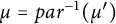 $\mu = par^{-1}(\mu ^{\prime })$
, we have
$\mu = par^{-1}(\mu ^{\prime })$
, we have
 $\mu \sim _R \lambda $
. The fact that our permutation
$\mu \sim _R \lambda $
. The fact that our permutation
 $(n_1, \ldots , n_{|\lambda |})$
was arbitrary implies that
$(n_1, \ldots , n_{|\lambda |})$
was arbitrary implies that
 $[\lambda ]_R$
includes a path of every color order; the fact that
$[\lambda ]_R$
includes a path of every color order; the fact that
 $par$
is injective implies that such a path is unique. Thus,
$par$
is injective implies that such a path is unique. Thus,
 $[\lambda ]_R$
satisfies (KG4), so Theorem 2.1 tells us that
$[\lambda ]_R$
satisfies (KG4), so Theorem 2.1 tells us that
 $\Lambda _R$
is a k-graph.
$\Lambda _R$
is a k-graph.
To see that
 $\Lambda _R$
is row-finite, it suffices to observe that
$\Lambda _R$
is row-finite, it suffices to observe that
 $|x \Lambda _R^{e_i}| = |par(x) \Lambda ^{e_i} | < \infty $
for all
$|x \Lambda _R^{e_i}| = |par(x) \Lambda ^{e_i} | < \infty $
for all
 $x \in \Lambda _R^0$
and for all
$x \in \Lambda _R^0$
and for all
 $1 \leq i\leq k$
. The fact that
$1 \leq i\leq k$
. The fact that
 $\Lambda _R$
is source-free follows from the analogous fact that
$\Lambda _R$
is source-free follows from the analogous fact that
 $0 \not = | \Lambda ^{e_i} par(x)| = |\Lambda ^{e_i}_R x|$
for all x and i. ▪
$0 \not = | \Lambda ^{e_i} par(x)| = |\Lambda ^{e_i}_R x|$
for all x and i. ▪
Theorem 6.4 If
 $(\Lambda , d)$
is a row-finite source-free k-graph, with
$(\Lambda , d)$
is a row-finite source-free k-graph, with
 $(\Lambda _R, d_R)$
the graph of
$(\Lambda _R, d_R)$
the graph of
 $\Lambda $
reduced at
$\Lambda $
reduced at
 $v \in \Lambda ^0$
, then
$v \in \Lambda ^0$
, then
 $C^*(\Lambda )$
is Morita equivalent to
$C^*(\Lambda )$
is Morita equivalent to
 $C^*(\Lambda _R)$
.
$C^*(\Lambda _R)$
.
Proof Let
 $\{ s_\lambda : \lambda \in \Lambda ^0 \cup \Lambda ^1 \}$
be the canonical Cuntz–Krieger
$\{ s_\lambda : \lambda \in \Lambda ^0 \cup \Lambda ^1 \}$
be the canonical Cuntz–Krieger
 $\Lambda $
-family generating
$\Lambda $
-family generating
 $C^*(\Lambda )$
. Define
$C^*(\Lambda )$
. Define
 $$ \begin{align*} T_\lambda = s_{par(\lambda)} \text{, for } \lambda \in \Lambda^0_R \cup \Lambda^1_R. \end{align*} $$
We first prove that
 $\{T_\lambda : \lambda \in \Lambda _R^0 \cup \Lambda _R^1 \}$
is a Cuntz–Krieger
$\{T_\lambda : \lambda \in \Lambda _R^0 \cup \Lambda _R^1 \}$
is a Cuntz–Krieger
 $\Lambda _R$
-family in
$\Lambda _R$
-family in
 $C^*(\Lambda )$
. Note that
$C^*(\Lambda )$
. Note that
 $\{ s_x : x \in \Lambda ^0 \}$
are nonzero and mutually orthogonal, and thus so are
$\{ s_x : x \in \Lambda ^0 \}$
are nonzero and mutually orthogonal, and thus so are
 $\{ T_x : x \in \Lambda _R^0 \}$
. Thus,
$\{ T_x : x \in \Lambda _R^0 \}$
. Thus,
 $\{ T_\lambda : \lambda \in \Lambda ^0_R \cup \Lambda ^1_R \}$
satisfies (CK1). Furthermore, if
$\{ T_\lambda : \lambda \in \Lambda ^0_R \cup \Lambda ^1_R \}$
satisfies (CK1). Furthermore, if
 $ab, cd \in G_R^*$
such that
$ab, cd \in G_R^*$
such that
 $ab \sim _R cd$
, then
$ab \sim _R cd$
, then
 $[ par(a) par(b)] =[par(ab)] = [par(cd)] = [par(c) par(d)]$
. By (KG0), we therefore have
$[ par(a) par(b)] =[par(ab)] = [par(cd)] = [par(c) par(d)]$
. By (KG0), we therefore have
 $$ \begin{align*} T_a T_b = s_{par(a)} s_{par(b)} = s_{par(c)} s_{par(d)} = T_c T_d, \end{align*} $$
and therefore
 $\{ T_\lambda : \lambda \in \Lambda ^0 \cup \Lambda ^1 \}$
satisfies (CK2). Now, fix
$\{ T_\lambda : \lambda \in \Lambda ^0 \cup \Lambda ^1 \}$
satisfies (CK2). Now, fix
 $e \in \Lambda _R^1$
. If
$e \in \Lambda _R^1$
. If
 $r(\iota (e)) \not = v$
, we have
$r(\iota (e)) \not = v$
, we have
 $\iota (e) = par(e)$
and hence
$\iota (e) = par(e)$
and hence
 $$ \begin{align*} T_e^* T_e = s_{par(e)}^* s_{par(e)} = s_{s(par(e))} = s_{par(s(e))} = T_{s(e)}. \end{align*} $$
If
 $r(\iota (e)) = v$
, then we similarly have
$r(\iota (e)) = v$
, then we similarly have
 $$ \begin{align*} T_e^* T_e = (s_f s_{e})^* (s_f s_{e}) = s_{e}^* s_f^* s_f s_{e} = s_{e}^* s_v s_{e} = s_{s(e)} = T_{s(e)}. \end{align*} $$
Therefore,
 $\{ T_\lambda : \lambda \in \Lambda ^0_R \cup \Lambda ^1_R \}$
satisfies (CK3).
$\{ T_\lambda : \lambda \in \Lambda ^0_R \cup \Lambda ^1_R \}$
satisfies (CK3).
Finally, to see that
 $\{ T_\lambda : \lambda \in \Lambda ^0_R \cup \Lambda ^1_R \}$
satisfies (CK4), we begin by considering (CK4) for
$\{ T_\lambda : \lambda \in \Lambda ^0_R \cup \Lambda ^1_R \}$
satisfies (CK4), we begin by considering (CK4) for
 $x \in \Lambda _R^0$
such that
$x \in \Lambda _R^0$
such that
 $x \neq w (= r(\Lambda ^1 v))$
. Note that for any basis vector
$x \neq w (= r(\Lambda ^1 v))$
. Note that for any basis vector
 $e_i \in \mathbb {N}^{k}$
,
$e_i \in \mathbb {N}^{k}$
,
 $$ \begin{align*} \sum\limits_{\substack{r_R(e) = x \\ d_R(e) = e_i}} T_e T_e^* = \sum\limits_{\substack{r_R(e) = x \\ d_R(e) = e_i}} s_{e} s_{e}^* = \sum\limits_{\substack{r(e) =x \\ d(e) = e_i}} s_e s_e^* = s_{x} = s_{par(x)} = T_x. \end{align*} $$
Thus, (CK4) holds for such vertices x.
In order to complete the proof that (CK4) holds, we first need a better understanding of the equivalence relation
 $\sim $
for paths which pass through
$\sim $
for paths which pass through
 $v\in \Lambda ^0$
. Because
$v\in \Lambda ^0$
. Because
 $v \Lambda ^1$
and
$v \Lambda ^1$
and
 $\Lambda ^1 v$
are complete edges by hypothesis, each set contains precisely one edge of each color. Thus, if we write
$\Lambda ^1 v$
are complete edges by hypothesis, each set contains precisely one edge of each color. Thus, if we write
 $g_{i} $
for the edge in
$g_{i} $
for the edge in
 $ v\Lambda ^1$
with
$ v\Lambda ^1$
with
 $d(g_{i}) = e_{i}$
and
$d(g_{i}) = e_{i}$
and
 $h_{i} $
for the edge in
$h_{i} $
for the edge in
 $\Lambda ^1 v$
such that
$\Lambda ^1 v$
such that
 $d(h_{i}) = e_{i}$
, then
$d(h_{i}) = e_{i}$
, then
 $s_v = s_{g_i} s_{g_i}^*$
for any i. Moreover, by our hypothesis that
$s_v = s_{g_i} s_{g_i}^*$
for any i. Moreover, by our hypothesis that
 $v\Lambda ^1$
and
$v\Lambda ^1$
and
 $\Lambda ^1 v$
are both complete edges, we have, for any
$\Lambda ^1 v$
are both complete edges, we have, for any
 $1 \leq i, j \leq k$
,
$1 \leq i, j \leq k$
,
 $$ \begin{align*} h_j g_i \sim h_i g_j &\implies s_{h_j} s_{g_i} = s_{h_i} s_{g_j} \implies s_{h_j} s_{g_i} s_{g_i}^* = s_{h_i} s_{g_j} s_{g_i}^* \\ &\implies s_{h_j} = s_{h_i} s_{g_j} s_{g_i}^*. \end{align*} $$
Thus, because
 $f = h_j$
for a unique j,
$f = h_j$
for a unique j,
 $$ \begin{align*} s_f s_f^* = (s_{h_i}s _{g_j} s_{g_i}^*) (s_{h_i} s_{g_j} s_{g_i}^*)^* = s_{h_i} s_{g_j} s_{g_i}^* s_{g_i} s_{g_j}^* s_{h_i}^* = s_{h_i} s_{h_i}^* \end{align*} $$
for all i. It follows that
 $$ \begin{align*} \sum\limits_{\substack{r_R(e) = w \\ d_R(e) = e_{i}}} T_e T_e^* &= T_{g_i} T_{g_i}^* + \sum\limits_{\substack{r_R(e) = w \\ e \neq g_i \\ d_R(e) = e_{i}}} T_e T_e^* = (s_f s_{g_i}) (s_f s_{g_i})^* + \sum\limits_{\substack{e \in w \Lambda^{e_i} \\ s(e) \neq v }} s_e s_e^* \\ &= s_{h_i} s_{h_i}^* + \sum\limits_{\substack{e \in w\Lambda^{e_i} \\ s(e) \neq v }} s_e s_e^* = \sum\limits_{\substack{e \in w\Lambda^{e_i}}} s_e s_e^* = s_{w} = T_w. \end{align*} $$
Therefore,
 $\{ T_\lambda : \lambda \in \Lambda ^0_R \cup \Lambda ^1_R \}$
satisfies (CK4), and thus is a Cuntz–Krieger
$\{ T_\lambda : \lambda \in \Lambda ^0_R \cup \Lambda ^1_R \}$
satisfies (CK4), and thus is a Cuntz–Krieger
 $\Lambda _R$
-family in
$\Lambda _R$
-family in
 $C^*(\Lambda )$
. By the universal property of
$C^*(\Lambda )$
. By the universal property of
 $C^*(\Lambda _R),$
there exists a homomorphism
$C^*(\Lambda _R),$
there exists a homomorphism
 $\pi :C^*(\Lambda _R) \rightarrow C^*(\Lambda )$
such that if
$\pi :C^*(\Lambda _R) \rightarrow C^*(\Lambda )$
such that if
 $C^*(\Lambda _R) = C^*(\{ t_\lambda : \lambda \in \Lambda ^0_R \cup \Lambda ^1_R\})$
, we have
$C^*(\Lambda _R) = C^*(\{ t_\lambda : \lambda \in \Lambda ^0_R \cup \Lambda ^1_R\})$
, we have
 $\pi (t_\lambda ) = T_\lambda $
for all
$\pi (t_\lambda ) = T_\lambda $
for all
 $\lambda \in \Lambda _R^0 \cup \Lambda _R^1$
. The computation above shows that our choice of edge f does not affect the validity of the construction.
$\lambda \in \Lambda _R^0 \cup \Lambda _R^1$
. The computation above shows that our choice of edge f does not affect the validity of the construction.
We now use the gauge-invariant uniqueness theorem and Lemma 2.5 to prove that
 $\pi $
is injective. If G is the 1-skeleton of
$\pi $
is injective. If G is the 1-skeleton of
 $\Lambda $
, we define
$\Lambda $
, we define
 $R:G^* \to \mathbb {Z}^k$
by
$R:G^* \to \mathbb {Z}^k$
by
 $$ \begin{align*} & R(e) = d(e) \text{, for } e \in \Lambda^1 \text{ s.t. } s(e) \neq v, \\ & R(e) = d(e) - d(f) \text{, for } e \in \Lambda^1 \text{ s.t. } s(e) = v, \\ & R(\lambda) = \sum_{i = 1}^{|\lambda|}R(\lambda_i) \text{, for } \lambda = \lambda_{|\lambda|} \cdots \lambda_2 \lambda_1 \in G^*, \\ & R(x) = 0 \text{, for } x \in \Lambda^0. \end{align*} $$
To show that R induces a well-defined function on
 $\Lambda $
, suppose that
$\Lambda $
, suppose that
 $\mu \sim \nu $
and consider
$\mu \sim \nu $
and consider
 $R(\mu ), R(\nu )$
. If
$R(\mu ), R(\nu )$
. If
 $s(\mu _i) = v$
, then the fact that
$s(\mu _i) = v$
, then the fact that
 $\Lambda ^1 v$
is a complete edge implies that
$\Lambda ^1 v$
is a complete edge implies that
 $s(\nu _i) = v$
. Therefore,
$s(\nu _i) = v$
. Therefore,
 $R(\mu ) = d(\mu ) - l \cdot d(f)$
and
$R(\mu ) = d(\mu ) - l \cdot d(f)$
and
 $R(\nu ) = d(\nu ) - l \cdot d(f)$
, where
$R(\nu ) = d(\nu ) - l \cdot d(f)$
, where
 $l \in \mathbb {N}$
counts the number of edges in
$l \in \mathbb {N}$
counts the number of edges in
 $\mu $
with source v. Because
$\mu $
with source v. Because
 $d(\mu ) = d(\nu )$
, we conclude
$d(\mu ) = d(\nu )$
, we conclude
 $R(\mu ) = R(\nu )$
. Thus, the function
$R(\mu ) = R(\nu )$
. Thus, the function
 $\beta : \mathbb {T}^{k} \to \text {Aut}(C^*(\Lambda ))$
defined by
$\beta : \mathbb {T}^{k} \to \text {Aut}(C^*(\Lambda ))$
defined by
 $\beta _z(s_{\mu }s_{\nu }^*) = z^{R(\mu ) - R(\nu )} s_{\mu }s_{\nu }^*$
is an action by Lemma 2.5.
$\beta _z(s_{\mu }s_{\nu }^*) = z^{R(\mu ) - R(\nu )} s_{\mu }s_{\nu }^*$
is an action by Lemma 2.5.
Let
 $\alpha $
be the canonical gauge action on
$\alpha $
be the canonical gauge action on
 $C^*(\Lambda _R)$
. For any
$C^*(\Lambda _R)$
. For any
 $e \in \Lambda ^1_R$
,
$e \in \Lambda ^1_R$
,
 $s(\iota (e)) \neq v$
, so
$s(\iota (e)) \neq v$
, so
 $R(\iota (e)) = d(\iota (e)) = d_R(e)$
. Moreover, if
$R(\iota (e)) = d(\iota (e)) = d_R(e)$
. Moreover, if
 $r(\iota (e)) \not = v$
, then
$r(\iota (e)) \not = v$
, then
 $\iota (e) = par(e)$
and
$\iota (e) = par(e)$
and
 $\pi (t_e) = s_{\iota (e)}$
, and so for any
$\pi (t_e) = s_{\iota (e)}$
, and so for any
 $z \in {\mathbb T}^k$
,
$z \in {\mathbb T}^k$
,
 $$ \begin{align*} \pi(\alpha_z(t_e)) &= \pi(z^{d_R(e)}t_e) = z^{d(\iota(e))}T_e = z^{d(\iota(e))}s_{\iota(e)} = z^{R(\iota(e))}s_{\iota(e)}\\ &= \beta_z(s_{par(e)}) = \beta_z(\pi(t_e)). \end{align*} $$
If
 $r(\iota (e)) = v,$
we have
$r(\iota (e)) = v,$
we have
 $$ \begin{align*} \pi(\alpha_z(t_e)) = \pi(z^{d_R(e)}t_e) &= z^{d_R(e)}T_e = z^{d(\iota(e))} s_f s_{\iota(e)} = z^{R(f)}z^{R(e)} s_f s_{\iota(e)} \\ &= \beta_z(s_f s_{\iota(e)}) = \beta_z(T_e) = \beta_z(\pi(t_e)). \end{align*} $$
It is straightforward to check that
 $\alpha _z$
and
$\alpha _z$
and
 $\beta _z$
also commute on the vertex projections. Therefore,
$\beta _z$
also commute on the vertex projections. Therefore,
 $\pi $
intertwines
$\pi $
intertwines
 $\beta $
with the canonical gauge action on
$\beta $
with the canonical gauge action on
 $C^*(\Lambda _R)$
and thus, by the gauge-invariant uniqueness theorem,
$C^*(\Lambda _R)$
and thus, by the gauge-invariant uniqueness theorem,
 $\pi $
is injective.
$\pi $
is injective.
We now use Theorem 2.6 to show that
 $\text {Im}\, (\pi ) \cong C^*(\Lambda _R)$
is Morita equivalent to
$\text {Im}\, (\pi ) \cong C^*(\Lambda _R)$
is Morita equivalent to
 $C^*(\Lambda )$
. Define
$C^*(\Lambda )$
. Define
 $X:= \Lambda ^0 \backslash \{ v\} $
and set
$X:= \Lambda ^0 \backslash \{ v\} $
and set
 $P_X = \sum _{x \in X} s_x \in M(C^*(\Lambda ))$
. Our first goal is to show that
$P_X = \sum _{x \in X} s_x \in M(C^*(\Lambda ))$
. Our first goal is to show that
 $P_X C^*(\Lambda ) P_X = \text {Im}(\pi )$
.
$P_X C^*(\Lambda ) P_X = \text {Im}(\pi )$
.
To see that
 $\text {Im}(\pi ) \subseteq P_X C^*(\Lambda ) P_X$
, recall that if
$\text {Im}(\pi ) \subseteq P_X C^*(\Lambda ) P_X$
, recall that if
 $\lambda \in \Lambda _R$
, then the vertices
$\lambda \in \Lambda _R$
, then the vertices
 $par(s_R(\lambda )) = s(par(\lambda )), par(r_R(\lambda )) = r(par(\lambda ))$
both lie in
$par(s_R(\lambda )) = s(par(\lambda )), par(r_R(\lambda )) = r(par(\lambda ))$
both lie in
 $ X$
. It follows that
$ X$
. It follows that
 $T_\lambda \in P_X C^*(\Lambda ) P_X$
for all
$T_\lambda \in P_X C^*(\Lambda ) P_X$
for all
 $\lambda \in \Lambda _R$
:
$\lambda \in \Lambda _R$
:
 $$ \begin{align*} T_\lambda = s_{par(\lambda)} = s_{r(par(\lambda))} s_{par(\lambda)} s_{s(par(\lambda))} = P_X s_{par(\lambda)} P_X. \end{align*} $$
Thus,
 $\pi (C^*(\Lambda _R)) \subseteq P_X C^*(\Lambda ) P_X.$
For the other inclusion, note that
 $$ \begin{align*}P_X C^*(\Lambda) P_X = \overline{\text{span}} \{ s_\lambda s_\mu^* : \mu, \lambda \in G^*,\, s(\mu) = s(\lambda), \, r(\lambda), r(\mu)\in X \}.\end{align*} $$
We will show that each such generator
 $s_\lambda s_\mu ^*$
is in
$s_\lambda s_\mu ^*$
is in
 $\text {Im}(\pi )$
. We begin with the following special case.
$\text {Im}(\pi )$
. We begin with the following special case.
Claim 1:
 $s_{h_i} s_{h_j}^* \in \text {Im}(\pi )$
for all edges
$s_{h_i} s_{h_j}^* \in \text {Im}(\pi )$
for all edges
 $h_i , h_j \in \Lambda ^1 v$
.
$h_i , h_j \in \Lambda ^1 v$
.
To see this, recall that
 $s_{h_i} = s_{h_j} s_{g_i} s_{g_j}^*$
, and so
$s_{h_i} = s_{h_j} s_{g_i} s_{g_j}^*$
, and so
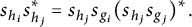 $$ \begin{align} s_{h_i} s_{h_j}^* = s_{h_j} s_{g_i} (s_{h_j} s_{g_j})^*. \end{align} $$
Now, write
 $e_\ell = d(f)$
. If
$e_\ell = d(f)$
. If
 $\ell = j$
, then
$\ell = j$
, then
 $s_{h_j} s_{g_i} = T_{\iota ^{-1}(g_i)} \in \text {Im}(\pi )$
and
$s_{h_j} s_{g_i} = T_{\iota ^{-1}(g_i)} \in \text {Im}(\pi )$
and
 $s_{h_j} s_{g_j} = T_{\iota ^{-1}(g_j)}$
, so
$s_{h_j} s_{g_j} = T_{\iota ^{-1}(g_j)}$
, so
 $s_{h_i} s_{h_j}^* \in \text {Im}(\pi )$
. Thus, we suppose
$s_{h_i} s_{h_j}^* \in \text {Im}(\pi )$
. Thus, we suppose
 $\ell \not = j$
.
$\ell \not = j$
.
By appealing to the results of Section 5, without loss of generality, we may assume that
 $w = r(h_j)$
is not an
$w = r(h_j)$
is not an
 $e_\ell $
sink. Thus, there is an edge
$e_\ell $
sink. Thus, there is an edge
 $e \in \Lambda ^{e_\ell } w$
. Because
$e \in \Lambda ^{e_\ell } w$
. Because
 $\Lambda ^1 v$
is a complete edge, we must have
$\Lambda ^1 v$
is a complete edge, we must have
 $e h_j \sim h f$
for some edge h. It follows that
$e h_j \sim h f$
for some edge h. It follows that
 $$ \begin{align*} s_{h_j} s_{g_i} = s_w s_{h_j} s_{g_i} = s_e^* s_e s_{h_j} s_{g_i} = s_e^* s_h s_f s_{g_i} .\end{align*} $$
If
 $r(e) = r(h) \in X$
, then
$r(e) = r(h) \in X$
, then
 $e = par(\iota ^{-1}(e))$
and
$e = par(\iota ^{-1}(e))$
and
 $h f g_i = par(\iota ^{-1}(h) \iota ^{-1}(g_i))$
. Consequently, in this case, we have
$h f g_i = par(\iota ^{-1}(h) \iota ^{-1}(g_i))$
. Consequently, in this case, we have
 $$ \begin{align*} s_{h_j} s_{g_i} = s_e^* T_{\iota^{-1}(h)} T_{\iota^{-1}(g_i)} = T_{\iota^{-1}(e)}^*T_{\iota^{-1}(h)} T_{\iota^{-1}(g_i)} \in \text{Im}(\pi).\end{align*} $$
If
 $r(e) = r(h) = v$
, then writing
$r(e) = r(h) = v$
, then writing
 $s_v = s_f^* s_f$
, we have
$s_v = s_f^* s_f$
, we have
 $$ \begin{align*} s_e^* s_{hf g_i} = (s_f s_e)^* s_{f h} s_{f g_i} = T_{\iota^{-1}(e)}^* T_{\iota^{-1}(h)} T_{\iota^{-1}(g_i)} \in \text{Im}(\pi).\end{align*} $$
Similarly, we compute that
 $s_{h_j} s_{g_j} = T_{\iota ^{-1}(e)}^* T_{\iota ^{-1}(h)} T_{\iota ^{-1}(g_j)} \in \text {Im}(\pi ).$
Equation (6.1) then implies that
$s_{h_j} s_{g_j} = T_{\iota ^{-1}(e)}^* T_{\iota ^{-1}(h)} T_{\iota ^{-1}(g_j)} \in \text {Im}(\pi ).$
Equation (6.1) then implies that
 $s_{h_i} s_{h_j}^* \in \text {Im}(\pi )$
for all
$s_{h_i} s_{h_j}^* \in \text {Im}(\pi )$
for all
 $1 \leq i, j \leq k$
, so Claim 1 holds.
$1 \leq i, j \leq k$
, so Claim 1 holds.
Next, we establish our second claim via a case-by-case analysis.
Claim 2: If
 $\eta \in G^*$
and
$\eta \in G^*$
and
 $s(\eta ) \not = v$
, then
$s(\eta ) \not = v$
, then
 $s_\eta \in \text {Im}(\pi )$
.
$s_\eta \in \text {Im}(\pi )$
.
To see this, note first that if v does not lie on
 $\eta $
, then
$\eta $
, then
 $\eta = par(\iota ^{-1}(\eta ))$
, so
$\eta = par(\iota ^{-1}(\eta ))$
, so
 $T_{\iota ^{-1}(\eta )} = s_\eta \in P_X C^*(\Lambda ) P_X$
.
$T_{\iota ^{-1}(\eta )} = s_\eta \in P_X C^*(\Lambda ) P_X$
.
If v lies on
 $\eta $
, and
$\eta $
, and
 $\eta \sim \rho $
, then the fact that
$\eta \sim \rho $
, then the fact that
 $\Lambda ^1 v, v \Lambda ^1$
are complete edges means that
$\Lambda ^1 v, v \Lambda ^1$
are complete edges means that
 $\rho $
will also pass through v. If
$\rho $
will also pass through v. If
 $\rho \sim \eta $
is such that every edge of
$\rho \sim \eta $
is such that every edge of
 $\rho $
with source v is f, then
$\rho $
with source v is f, then
 $\rho \in \text {Im}(par)$
and therefore
$\rho \in \text {Im}(par)$
and therefore
 $s_\rho = s_\eta \in \text {Im}(\pi )$
.
$s_\rho = s_\eta \in \text {Im}(\pi )$
.
For the last case, suppose that v lies on
 $\eta $
but that for every path
$\eta $
but that for every path
 $\rho $
with
$\rho $
with
 $\rho \sim \eta $
, there is an edge
$\rho \sim \eta $
, there is an edge
 $\rho _i$
in
$\rho _i$
in
 $\rho $
with
$\rho $
with
 $s(\rho _i) = v$
and
$s(\rho _i) = v$
and
 $\rho _i \not = f$
. Without loss of generality, suppose that i is the smallest such. By hypothesis,
$\rho _i \not = f$
. Without loss of generality, suppose that i is the smallest such. By hypothesis,
 $s(\eta ) = s(\rho ) \not = v$
, so
$s(\eta ) = s(\rho ) \not = v$
, so
 $i \not = 1.$
As established in the proof of Claim 1,
 $ s_{\rho _i} = s_e^* s_h s_f$
for edges e of degree
$ s_{\rho _i} = s_e^* s_h s_f$
for edges e of degree
 $d(f)$
and h of degree
$d(f)$
and h of degree
 $d(\rho _i)$
, and we have
$d(\rho _i)$
, and we have
 $$ \begin{align*} s_{\rho_i} s_{\rho_{i-1}} = s_e^* s_{h f \rho_{i-1}} \in \text{Im}(\pi).\end{align*} $$
By construction,
 $\rho _{i-2} \cdots \rho _1$
does not pass through v, and so
$\rho _{i-2} \cdots \rho _1$
does not pass through v, and so
 $s_{\rho _{i-2} \cdots \rho _1} \in \text {Im}(\pi )$
. An inductive application of this argument now shows that
$s_{\rho _{i-2} \cdots \rho _1} \in \text {Im}(\pi )$
. An inductive application of this argument now shows that
 $s_\rho = s_\eta $
lies in
$s_\rho = s_\eta $
lies in
 $\text {Im}(\pi )$
whenever
$\text {Im}(\pi )$
whenever
 $s(\eta ) \not = v$
. This completes the proof of Claim 2.
$s(\eta ) \not = v$
. This completes the proof of Claim 2.
Finally, consider an arbitrary generator
 $s_\lambda s_\mu ^*$
of
$s_\lambda s_\mu ^*$
of
 $P_X C^*(\Lambda ) P_X$
, with
$P_X C^*(\Lambda ) P_X$
, with
 $\lambda = \lambda _{|\lambda |} \cdots \lambda _1, \mu = \mu _{|\mu |} \cdots \mu _1 \in G^*$
. If
$\lambda = \lambda _{|\lambda |} \cdots \lambda _1, \mu = \mu _{|\mu |} \cdots \mu _1 \in G^*$
. If
 $s(\lambda ) = s(\mu ) \not = v$
, then applying Claim 2 to
$s(\lambda ) = s(\mu ) \not = v$
, then applying Claim 2 to
 $\lambda $
and
$\lambda $
and
 $\mu $
, we see that
$\mu $
, we see that
 $s_\lambda s_\mu ^* \in \text {Im}(\pi )$
. If
$s_\lambda s_\mu ^* \in \text {Im}(\pi )$
. If
 $v = s(\lambda ) = s(\mu ),$
then by Claim 1,
$v = s(\lambda ) = s(\mu ),$
then by Claim 1,
 $s_{\lambda _1} s_{\mu _1}^* \in \text {Im}(\pi )$
. Because
$s_{\lambda _1} s_{\mu _1}^* \in \text {Im}(\pi )$
. Because
 $r(\lambda _1) = r(\mu _1) = w \not = v$
, it follows from Claim 2 that if
$r(\lambda _1) = r(\mu _1) = w \not = v$
, it follows from Claim 2 that if
 $\eta := \lambda _{|\lambda |} \cdots \lambda _2$
and
$\eta := \lambda _{|\lambda |} \cdots \lambda _2$
and
 $\zeta := \mu _{|\mu |} \cdots \mu _2$
, then
$\zeta := \mu _{|\mu |} \cdots \mu _2$
, then
 $s_\eta , s_\zeta \in \text {Im}(\pi )$
. Consequently,
$s_\eta , s_\zeta \in \text {Im}(\pi )$
. Consequently,
 $s_\lambda s_\mu ^* = s_\eta s_{\lambda _1} s_{\mu _1}^* s_\zeta ^* \in \text {Im}(\pi )$
for any generator
$s_\lambda s_\mu ^* = s_\eta s_{\lambda _1} s_{\mu _1}^* s_\zeta ^* \in \text {Im}(\pi )$
for any generator
 $s_\lambda s_\mu ^*$
of
$s_\lambda s_\mu ^*$
of
 $P_X C^*(\Lambda ) P_X$
.
$P_X C^*(\Lambda ) P_X$
.
Having established that
 $P_X C^*(\Lambda ) P_X = \text {Im}(\pi ) \cong C^*(\Lambda _R)$
, we now compute the saturation
$P_X C^*(\Lambda ) P_X = \text {Im}(\pi ) \cong C^*(\Lambda _R)$
, we now compute the saturation
 $\Sigma (X)$
in order to apply Theorem 2.6. Note that
$\Sigma (X)$
in order to apply Theorem 2.6. Note that
 $w \in X$
and there are edges
$w \in X$
and there are edges
 $h_j$
in
$h_j$
in
 $w \Lambda ^1 v$
, so any hereditary set containing X must also contain v. Thus,
$w \Lambda ^1 v$
, so any hereditary set containing X must also contain v. Thus,
 $\Sigma (X) = \Lambda ^0$
. Theorem 2.6 therefore tells us that
$\Sigma (X) = \Lambda ^0$
. Theorem 2.6 therefore tells us that
 $C^*(\Lambda ) \sim _{ME} C^*(\Lambda _R)$
, as claimed. ▪
$C^*(\Lambda ) \sim _{ME} C^*(\Lambda _R)$
, as claimed. ▪
Acknowledgment
We would like to express our sincere gratitude for Kenton Ke, Emily Morison, Jethro Thorne, and Ryan Wood for helpful comments.


 Open access