


Nomenclature
- $\bar c$
-
mean aerodynamic chord
-
${c_i}$
-
controller gain parameter,
$i = 1,2$
-
${C_D}$
-
drag coefficient
-
${C_L}$
-
lift coefficient
-
${C_M}$
-
pitching moment coefficient
-
${C_T}$
-
thrust coefficient
-
$d$
-
external disturbance
-
$D$
-
drag force
- FDD
-
fault detection and diagnosis
- FPA
-
flight-path angle
- FTC
-
fault-tolerant control
-
$h$
-
flight altitude
-
${h_d}$
-
desired flight altitude
-
${h_{df}}$
-
filtered desired flight altitude
- HFV
-
hypersonic flight vehicle
-
${I_{yy}}$
-
moment of inertia about pitch axis
-
${k_1}$
-
controller design parameter
-
${k_2}$
-
controller design parameter
-
${k_h}$
-
flight-path angle command proportional coefficient
-
${k_i}$
-
flight-path angle command integral coefficient
-
$L$
-
lift force
-
$m$
-
mass of aircraft
-
${M_{yy}}$
-
pitch moment
- PID
-
proportional integral derivative
-
$q$
-
pitch rate
-
$\bar q$
-
dynamic pressure
-
$r$
-
the radial distance from earth’s centre
-
$S$
-
reference area
-
$T$
-
thrust force
-
$u$
-
system control input
-
$v$
-
desired control input
-
$V$
-
mass-centre velocity
-
$x_i^F$
-
actual sensor measured values of system state
-
${z_i}$
-
state error,
$i = 1,2,3$
-
$\alpha $
-
angle-of-attack
-
${\alpha _1}$
-
designed virtual control variable
-
${\alpha _2}$
-
designed virtual control variable
-
$\gamma $
-
flight-path angle
-
${\gamma _d}$
-
desired flight-path angle
-
${\gamma _i}$
-
adaptive law parameter,
$i = 1,2$
-
${\delta _e}$
-
elevator deflection
-
$\varepsilon $
-
robust term parameter
-
$\theta $
-
pitch angle
-
$\mu $
-
the gravitational constant
-
$\rho $
-
air density
-
${\rho _i}$
-
effectiveness loss fault coefficient,
$i = 0,1,2,3$
-
$\sigma $
-
control gain direction
-
$\varphi $
-
bias fault coefficient


1.0 Introduction
This paper focuses on the design of fault-tolerant control (FTC) problem for hypersonic flight vehicle (HFV), including considerations of unknown sensor fault, unknown time-varying fault and control direction of actuator and the influence of varying external disturbance, which is a challenging study in HFV field. The structure of the paper is organised as follows. Section 1.0 introduces the HFV system and reviews FTC methods, concluding with a summary of the key contributions of this study. Section 2.0 presents the control-oriented dynamics model of HFV system and provides some associated lemmas and assumptions. In Section 3.0, the adaptive backstepping fault-tolerant controller design scheme and detailed steps are discussed, and the Lyapunov method is employed to prove the system stability. In Section 4.0, numerical simulations are carried out to verify the effectiveness of the proposed controller. Finally, concluding remarks of this paper are drawn in Section 5.0.
HFV refers to the vehicle at a speed of Mach 5 or above. Mach numbers are used to verify the speed compared to that of sound, which means the velocity of HFV is at least 5 times faster than the speed of sound. At this speed, it has huge application potential to develop in the military and civil fields. The hypersonic speed and large flight envelope of HFV confer significant advantages in military confrontations, enabling it to carry out global attacks and rapid emergency responses. These capabilities not only provide strategic deterrence, but also signify the arrival of an era of precise and swift weapons. Meanwhile, as a new type hypersonic transportation vehicle for passengers and cargos, HFV can greatly reduce travelling time and improve transport efficiency in remote deliveries, which can bring the large commercial value in civil carriage [Reference Ding, Yue, Chen and Si1, Reference Xu and Shi2]. In future, HFV also has strong applicability in space development by its reusability, providing more reliable and controllable tools that can realise multiple round trips from space, which significantly reduces the cost of space launch missions [Reference Sziroczak and Smith3].
As the key technology of HFV, controller design plays a pivotal role in ensuring optimal flight performance and successful task completion. However, unlike traditional sub-sonic aircraft, HFV has the unique airframe-scramjet integration design, resulting in a strong coupling effect between the propulsion and aerodynamic systems [Reference Serrani and Bolender4]. Additionally, the intricate characteristics of HFV’s dynamic model include strong nonlinearity, rapid time-varying behaviour and uncertainty in aerodynamic parameters, which all give rise to challenges in terms of controller design and stability analysis [Reference An, Wu, Wang, Kao and Wang5, Reference Shao, Shi and Zhang6]. For these problems of HFV, there are fruitful control methods which have been designed to enhance the control performance and flight quality, such as adaptive control [Reference An and Wu7–Reference Sun, Li, Guo, Wang and Li9], slide mode control [Reference Cao, Tang and Zhang10–Reference Wang, Bao and Li12], intelligent control [Reference Bu, He and Wang13–Reference Wang, An, Wang, Xia and Ma15] and so on.
It is well known that HFV has complex body structure for the need of hypersonic flight. Some mechanistic components such as actuators and sensors are equipped on the outer surface of the body to ensure the safety and controllability [Reference Cao, Gao, Qian and Zhao16, Reference Kienitz, Staats, Lohr, Irsperger, Schmid, Koch and Weiss17]. During the real hypersonic flight, the extreme high speed can generate lots of aerodynamic heat that will affect the structural strength of the aircraft. Meanwhile, the high dynamic harsh flight environment inevitably produces external disturbance for HFV. These structural damage and continuous interference can cause partial or complete faults on the actuators and sensors, which could further lead to hazards and safety accidents [Reference Zhu, Jiang and Yu18]. HFV is a highly refined and integrated weapon, which is quite vulnerable to suffer from these structural and component faults in hypersonic environment [Reference Yu, Li and Zhang19]. Therefore, it is crucial to guarantee system stability and improve the safety and reliability of HFV with sensor, actuator faults and external disturbance. In recent years, FTC techniques have been increasingly considered and studied in the controller design of HFV. Generally, FTC techniques can be divided into active and passive methods [Reference Xu, Guo, Yuan, Fan and Wang20]. The active FTC system possesses fault detection and diagnosis (FDD) scheme, which can provide information to the controller reconfiguration. In Ref. [Reference Zhao, Song, Ai, Xu and Liu21], Zhao et al. presented a novel active FTC strategy for handling actuator faults of near-space HFV. Their research was based on active disturbance rejection control combined with FDD, which supported effective command tracking and faults compensation. In Ref. [Reference Wu, Wang, Yu, Liu and Wu22], for over-actuated hypersonic vehicles, a hierarchical FTC mechanism composed of diagnosis and control layer was designed. Using diagnosed fault information, the robust control allocation method distributed the desired control moment to the actuator. However, the passive approach employs a fixed controller with strong robustness and adaptive ability, which can ensure system basic stable control and fault-tolerant performance with good flight quality when actuator or sensor faults occur. Because of its simple structure and convenience to design and implement, the passive FTC scheme is often adopted in many practical engineering applications like HFV [Reference Gao, Cai and Nan23]. In Ref. [Reference Zhao, Jiang, Yang and Tao24], a passive FTC method was proposed to address process faults and suppress vibrations for flexible HFV according to the bilinear matrix inequalities technique, and simulation results demonstrated its effectiveness. In Ref. [Reference Yue and Sun25], Yue et al. developed the robust anti-saturation FTC approaches for HFV to handle issues related to input saturation and actuator faults.
In Ref. [Reference Yu, Wang and Li26], Yu et al. developed an FTC strategy for attitude control of the hypersonic vehicle by incorporating actuator fault into lumped disturbance, which was estimated by a high order sliding mode observer. Similarly, the finite-time terminal sliding mode control approach was designed for the hypersonic gliding vehicle to deal with actuator faults and model uncertainties in [Reference Yu, Li and Zhang27]. In Ref. [Reference Zhu, Jiang and Yu18], based on the fault observer, a novel FTC approach was proposed to mitigate actuator effectiveness loss and bias fault for HFV. Lu et al. proposed a novel output feedback FTC method to settle the measurement and saturation problem of actuator in HFV system [Reference Lu, Jia, Liu and Lu28]. However, most of the previous studies involving FTC for HFV focused on the actuator faults. Sensors also play an important role during an actual hypersonic flight, which greatly influence the accurate measurement of system variables. Besides, if the sensor faults occur and are not handled efficiently, the actuators will receive the incorrect signals and maybe cause devastating consequences [Reference Shen, Jiang and Shi29]. Compared to the studies on actuators, there are fewer studies on sensor faults for the HFV [Reference Chen, Jiang and Wen30]. In Ref. [Reference Gao, Lin and Cao31], a robust fault-tolerant output feedback controller with an observer was proposed considering the sensor fault and external disturbance. Chen et al. developed a sensor cascading fault estimation method based on a novel multidimensional observer of HFV, and proposed an FTC approach that addressed the ineffectiveness of traditional observers in cascading faults [Reference Chen, Gong and Li32]. There are some existing studies that focused on controller design, considering both actuator and sensor faults. For linear systems, Lee et al. introduced virtual observers to enhance observation accuracy, and based on these, they designed an FTC scheme to solve problems of sensor and actuator faults [Reference Lee, Lim, Nahavandi and Roberts33]. For multi-input multi-output nonlinear systems in presence of unknown actuator and sensor faults, a fuzzy fault-tolerant tracking control scheme was developed based on a backstepping design framework [Reference Bounemeur, Chemachema and Essounbouli34]. In Ref. [Reference Liang, Wang, Hu and Dong35], Liang et al. investigated the attitude control problem in a satellite system. An output feedback FTC strategy was proposed to handle actuator and sensor faults based on the auxiliary observer.
However, in terms of the HFV system, although there have been plenty of studies on FTC for actuator and sensor faults separately, research on controller design that considers simultaneous faults in both actuators and sensors, as well as external disturbance, is still limited. An et al. introduced an adaptive FTC method for HFV considering components faults, uncertain parameters and flexible dynamics [Reference An, Wu, Wang and Cao36]. The model was derived with sensor and actuator faults, but the unknown control direction issues were not discussed in the study. The control direction is also called the sign of control gain direction, which indicates the motion direction of system under given control input and is typically assumed to be known. However, for HFV system, the intricate flight environment and the potential occurrence of reverse signal faults in massive telex components may result in sudden reversals in control gain direction, which could cause instability of system and even safety concerns if ignored [Reference Lv, Schutter, Wang and Shen37]. To guarantee the safety and reliability of HFV in extreme hypersonic flight environments, it is crucial to develop an effective FTC approach that can simultaneously handle various types of faults and external disturbance. Therefore, further study is needed in this area to improve fault tolerance and robustness of the HFV system.
The adaptive backstepping control is a powerful approach for design of various nonlinear and uncertain systems, particularly those in parameter strict feedback form [Reference Kokotovic38]. In the backstepping control [Reference Tran and Nguyen39], the high-order system can be recursively divided into several low-order subsystems step by step, making it more convenient to design the virtual control signals, which can reduce the controller design complexity. Besides, the adaptive algorithms have strong robustness and certain effectiveness without requiring additional systems, which is more practical in the engineering field [Reference Basri40, Reference Gao and Liu41]. In Ref. [Reference Liu, Jiang, Mao and Ding42], Liu et al. designed an adaptive backstepping controller that addressed the problems of unknown system parameters, actuator faults and disturbance for high-speed trains. In Ref. [Reference Gao, Zhang and Liu43], a new adaptive boundary control approach dealing with input constraints and disturbance was developed to suppress the deformations of the flexible wings. Anjum et al. utilised adaptive backstepping approach to design a finite-time FTC method for robotic manipulators considering unknown disturbances and actuator fault [Reference Anjum and Guo44]. Therefore, the adaptive backstepping control scheme has a great potential for exploring the FTC design for HFV.
The unknown control direction implies that the sign of control gain is unknown, and it could be either positive or negative. Under the same control input, opposite control direction might lead to significant difference. To address this problem, there are control approaches such as sliding mode control with monitoring function or observers, as well as the Nussbaum gain technique. Oliveira et al. designed an adaptive output-feedback controller based on a monitoring function, which solved the unknown control direction problem by diagnosing and adjusting the control sign [Reference Oliveira, Peixoto and Nunes45]. Guo et al. employed sliding mode technology combined with an adaptive disturbance observer to address the control issue [Reference Guo, Guo, Wang, Chang and Huang46]. However, the monitoring function is complex to design and the sliding mode control possesses chattering characteristic that could potentially damage the HFV system. The Nussbaum gain function was first put forward in Ref. [Reference Nussbaum47], which has been extensively adopted as a control gain estimator to handle unknown control direction problem [Reference Chang, Breuker and Wang48–Reference Huang, Wang, Wen and Zhou50]. Its fundamental principle is to alternatively change the sign of control force within an adaptive design framework. Furthermore, the technical lemma, which guarantees the boundedness of the Lyapunov function when its derivative along the system is upper bounded by a Nussbaum function-based type function, simplifies the proof of system stability [Reference Chen51]. Therefore, the Nussbaum gain function technique can be employed to address the singularity problem caused by unknown control direction of the actuator. By combining this technique with the adaptive backstepping control approach, the designed controller can effectively solve the problems of unknown actuator and sensor faults and unknown control direction under external disturbance.
Motivated by the above discussions, this study proposes a novel adaptive backstepping FTC strategy for HFV based on the Nussbaum gain function technique, which considers the different types of unknown actuator and sensor’s faults, unknown control direction and varying external disturbance. It improves traditional FTC methods that primarily take the actuator fault into consideration in HFV. Compared with the existing research studies, the key contributions can be summarised as follows:
-
(1) The designed controller is developed for the HFV system in the presence of unknown sensor fault, unknown time-varying fault and control direction of the actuator, and varying external disturbance. This approach offers more comprehensive consideration of multiple influential factors and holds greater practical significance compared to the studies that exclusively consider actuator faults in Ref. [Reference Zhu, Jiang and Yu18, Reference Yue and Sun25–Reference Lu, Jia, Liu and Lu28] or sensor faults in Ref. [Reference Chen, Jiang and Wen30–Reference Chen, Gong and Li32].
-
(2) Different from Ref. [Reference Zhao, Song, Ai, Xu and Liu21, Reference Wu, Wang, Yu, Liu and Wu22, Reference Shen, Jiang and Shi29, Reference Chen, Gong and Li32], the proposed control scheme consists of a simple controller without requiring the FDD system or controller reconfiguration. It has the certain robustness to adapt the unknown fault parameters and varying disturbance, which has wider applications in the field of HFV control.
-
(3) Based on the Nussbaum gain function technique, we design a novel FTC algorithm that can avoid the singularity problem and ensure the stability of the HFV system with unknown control direction, varying fault parameters and disturbance. Simulation results demonstrate that the proposed controller has superior control performance compared with traditional proportional integral derivative (PID) controller.
2.0 Problem statement
2.1 HFV basic model
In this paper, the HFV basic model under study is developed from the NASA Langley Research Centre [Reference Marrison and Stengel52]. We assume that HFV is a rigid body and ignore its elastic modes. The key angles of simplified model are shown in Fig. 1.
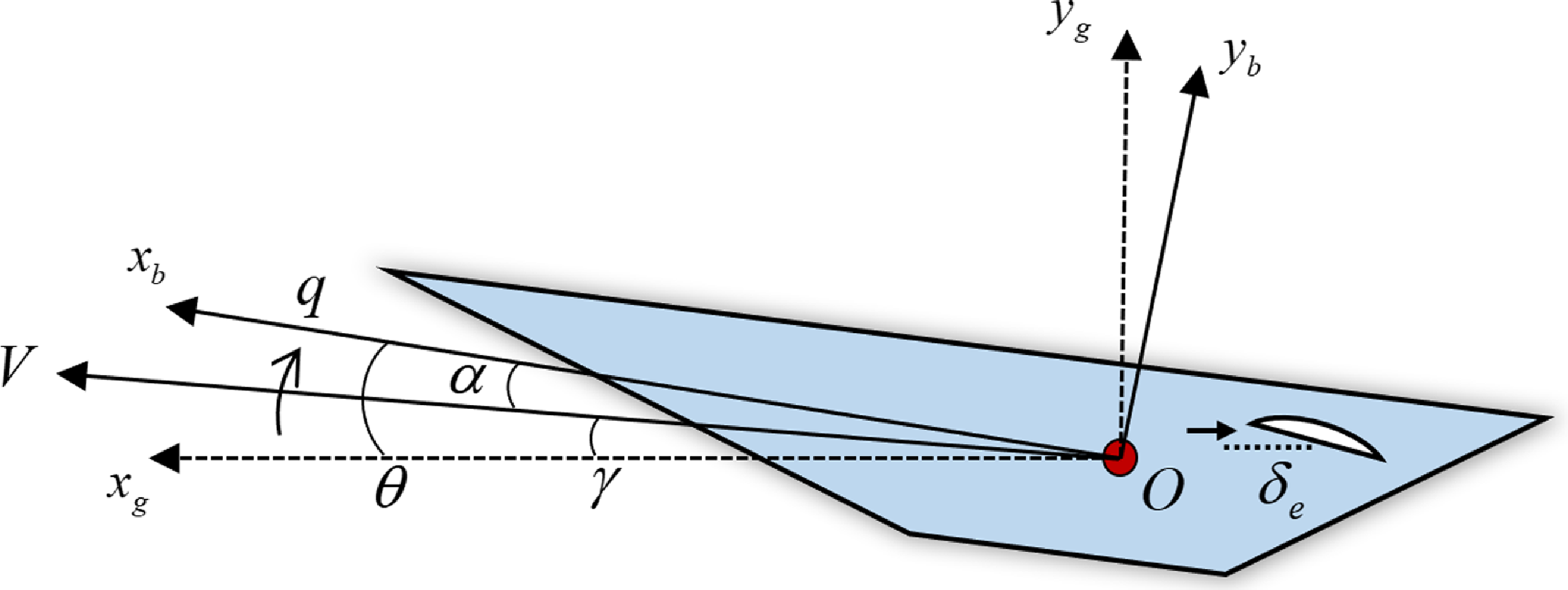
Figure 1. Simplified HFV model.
Where $O{x_g}{y_g}$
and
$O{x_g}{y_g}$
and $O{x_b}{y_b}$
denote the global inertial coordinate system and body axis coordinate system, respectively.
$O{x_b}{y_b}$
denote the global inertial coordinate system and body axis coordinate system, respectively. $V$
represents the mass-centre velocity of aircraft.
$V$
represents the mass-centre velocity of aircraft. $\gamma ,\alpha ,\theta $
are flight-path angle (FPA), angle-of-attack and pitch angle.
$\gamma ,\alpha ,\theta $
are flight-path angle (FPA), angle-of-attack and pitch angle. $q,{\delta _e}$
denote the pitch rate and the elevator deflection of HFV. Combined with the flight altitude
$q,{\delta _e}$
denote the pitch rate and the elevator deflection of HFV. Combined with the flight altitude $h$
of HFV, the longitudinal dynamic model can be described by the set of differential equations for
$h$
of HFV, the longitudinal dynamic model can be described by the set of differential equations for $V,h,\gamma ,\alpha ,q$
as follows
$V,h,\gamma ,\alpha ,q$
as follows
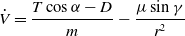 \begin{align} \dot V = \frac{{T\cos \alpha - D}}{m} - \frac{{\mu \sin \gamma }}{{{r^2}}}\end{align}
 \begin{align}\dot h = V\sin \gamma \end{align}
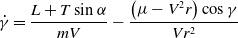 \begin{align}\dot \gamma = \frac{{L + T\sin \alpha }}{{mV}} - \frac{{\left( {\mu - {V^2}r} \right)\cos \gamma }}{{V{r^2}}}\end{align}
 \begin{align}\dot \alpha = q - \dot \gamma \end{align}
 \begin{align}\dot q = \frac{{{M_{yy}}}}{{{I_{yy}}}}\end{align}
where $m$
,
$m$
, $\mu $
,
$\mu $
, $r$
,
$r$
, ${I_{yy}}$
are the mass of HFV, the gravitational constant, the radial distance from Earth’s centre, and the moment of inertia about pitch axis, respectively. The lift
${I_{yy}}$
are the mass of HFV, the gravitational constant, the radial distance from Earth’s centre, and the moment of inertia about pitch axis, respectively. The lift $L$
, drag
$L$
, drag $D$
, thrust
$D$
, thrust $T$
and pitch moment
$T$
and pitch moment ${M_{yy}}$
can be formulated as follows
${M_{yy}}$
can be formulated as follows
 \begin{align}L = \bar qS{C_L}\end{align}
 \begin{align}D = \bar qS{C_D}\end{align}
 \begin{align}T = \bar qS{C_T}\end{align}
 \begin{align}{M_{yy}} = \bar qS\bar c\left( {{C_M}\left( \alpha \right) + {C_M}\left( q \right) + {C_M}\left( {{\delta _e}} \right)} \right)\end{align}
where $\bar q = \rho {V^2}/2$
denotes the dynamic pressure of HFV.
$\bar q = \rho {V^2}/2$
denotes the dynamic pressure of HFV. $\rho $
and
$\rho $
and $S$
represent the air density and the reference area, respectively. Applying the polynomial fitting of the aero coefficients near the equilibrium point, the aerodynamic forces and moments coefficients can be described as follows [Reference Shaughnessy, Pinckney, McMinn, Cruz and Kelley53]
$S$
represent the air density and the reference area, respectively. Applying the polynomial fitting of the aero coefficients near the equilibrium point, the aerodynamic forces and moments coefficients can be described as follows [Reference Shaughnessy, Pinckney, McMinn, Cruz and Kelley53]
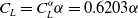 \begin{align}{C_L} = C_L^\alpha \alpha = 0.6203\alpha \end{align}
 \begin{align}{C_D} = 0.645{\alpha ^2} + 0.0043378\alpha + 0.003772\end{align}
 \begin{align}{C_T} = \left\{ \begin{array}{l}0.02576\beta \qquad\qquad\qquad {\rm{ if\ }}\beta \lt 1\\0.0224 + 0.00336\beta \qquad {\rm{ if\ }}\beta \gt 1{\rm{ }}\end{array} \right.\end{align}
 \begin{align}{C_M}(\alpha ) = - 0.035{\alpha ^2} + 0.036617\alpha + 5.3261 \times {10^{ - 6}}\end{align}
 \begin{align}{C_M}(q) = (\bar c/2V)q\left( { - 6.796{\alpha ^2} + 0.3015\alpha - 0.2289} \right)\end{align}
 \begin{align}{C_M}\left( {{\delta _e}} \right) = {c_e}\left( {{\delta _e} - \alpha } \right)\end{align}
where $\bar c$
denotes the mean aerodynamic chord. More parameter values and specific coefficient explanations about this model can be found in Ref. [Reference Xu, Mirmirani and Ioannou54].
$\bar c$
denotes the mean aerodynamic chord. More parameter values and specific coefficient explanations about this model can be found in Ref. [Reference Xu, Mirmirani and Ioannou54].
2.2 Control-oriented model and faults analysis
Assumption 2.1 The trust term $T\sin \alpha $
in Equation (3) is generally neglected because it is much smaller than
$T\sin \alpha $
in Equation (3) is generally neglected because it is much smaller than $L$
.
$L$
.
During straight and level flight, the nonlinear dynamics equations (1)–(5) can be linearised at the trim point. Based on Assumption 2.1, the HFV system can be divided into a velocity subsystem and an altitude subsystem. However, the velocity subsystem is a first-order system that can be controlled by a simple dynamic inversion approach, which is not the focus of control algorithms research in this paper.
Assumption 2.2 The reference altitude $h$
and its high derivates are known and bounded.
$h$
and its high derivates are known and bounded.
Assumption 2.3 Since $\gamma $
is quite small during the real hypersonic flight, we take
$\gamma $
is quite small during the real hypersonic flight, we take $\sin \gamma \approx \gamma $
,
$\sin \gamma \approx \gamma $
, $\cos \gamma \approx 1$
for simplification in the modelling.
$\cos \gamma \approx 1$
for simplification in the modelling.
For the altitude subsystem (2)–(5), it is noted that the mathematical relationship between altitude $h$
and FPA
$h$
and FPA $\gamma $
is analytical and unambiguous without any uncertainty. Therefore, the altitude control command can be converted into the FPA control command, which simplifies the control-oriented modelling and controller design. According to Assumption 2.3, we define the reference altitude command
$\gamma $
is analytical and unambiguous without any uncertainty. Therefore, the altitude control command can be converted into the FPA control command, which simplifies the control-oriented modelling and controller design. According to Assumption 2.3, we define the reference altitude command ${h_d}\left( t \right)$
, error
${h_d}\left( t \right)$
, error $\tilde h\left( t \right) = h\left( t \right) - {h_d}\left( t \right)$
. And the reference FPA command can be given as Ref. [Reference Xu, Yang and Pan55]
$\tilde h\left( t \right) = h\left( t \right) - {h_d}\left( t \right)$
. And the reference FPA command can be given as Ref. [Reference Xu, Yang and Pan55]
 \begin{align}{\gamma _d}\left( t \right) = \frac{{ - {k_h}\tilde h\left( t \right) - {k_i}\int {\tilde h\left( t \right) + {{\dot h}_d}\left( t \right)} }}{V}\end{align}
where ${k_h}$
and
${k_h}$
and ${k_i}$
are the positive design constants. Thus, there is
${k_i}$
are the positive design constants. Thus, there is $h\left( t \right) \to {h_d}\left( t \right)$
when
$h\left( t \right) \to {h_d}\left( t \right)$
when $\gamma \left( t \right) \to {\gamma _d}\left( t \right)$
.
$\gamma \left( t \right) \to {\gamma _d}\left( t \right)$
.
According to the angular interrelations among various coordinate systems, there are $\theta = \alpha + \gamma $
that can be observed in Fig. 1. Consequently, based on the subsystem (3)–(5), we choose FPA
$\theta = \alpha + \gamma $
that can be observed in Fig. 1. Consequently, based on the subsystem (3)–(5), we choose FPA $\gamma $
, pitch angle
$\gamma $
, pitch angle $\theta $
, and pitch rate
$\theta $
, and pitch rate $q$
as the system state variables to establish the control-oriented model, which are expressed as
$q$
as the system state variables to establish the control-oriented model, which are expressed as ${x_1} = \gamma $
,
${x_1} = \gamma $
, ${x_2} = \theta $
,
${x_2} = \theta $
, ${x_3} = q$
. Considering the external disturbance during the flight, the state space model can be transformed into the following from
${x_3} = q$
. Considering the external disturbance during the flight, the state space model can be transformed into the following from
 \begin{align}{\dot x_1} = {f_1}({x_1}) + {g_1}{x_2}\end{align}
 \begin{align}{\dot x_2} = {f_2} + {g_2}{x_3}\end{align}
 \begin{align}{\dot x_3} = {f_3}({x_1},{x_2},{x_3}) + {g_3}\left( {u(t) + d(t)} \right)\end{align}
where ${f_1}({x_1}) = {\varsigma _1}{x_1} + {\varsigma _2}\cos \left( {{x_1}} \right)$
,
${f_1}({x_1}) = {\varsigma _1}{x_1} + {\varsigma _2}\cos \left( {{x_1}} \right)$
, ${\varsigma _1} = - C_L^\alpha \bar qS/mV \lt 0$
,
${\varsigma _1} = - C_L^\alpha \bar qS/mV \lt 0$
, ${\varsigma _2} = - \left( {\mu - {V^2}r} \right)/V{r^2} \lt 0$
,
${\varsigma _2} = - \left( {\mu - {V^2}r} \right)/V{r^2} \lt 0$
, ${g_1} = C_L^\alpha \bar qS/mV$
,
${g_1} = C_L^\alpha \bar qS/mV$
, ${f_2} = 0$
,
${f_2} = 0$
, ${g_2} = 1$
,
${g_2} = 1$
, ${f_3}({x_1},{x_2},{x_3}) = \bar qS\bar c\left( {{C_M}\left( \alpha \right) + {C_M}\left( q \right) - {c_e}\alpha } \right)/{I_{yy}}$
,
${f_3}({x_1},{x_2},{x_3}) = \bar qS\bar c\left( {{C_M}\left( \alpha \right) + {C_M}\left( q \right) - {c_e}\alpha } \right)/{I_{yy}}$
, ${g_3} = \bar qS\bar c{c_e}/{I_{yy}}$
. The system control input
${g_3} = \bar qS\bar c{c_e}/{I_{yy}}$
. The system control input $u\left( t \right) = {\delta _e}\left( t \right)$
.
$u\left( t \right) = {\delta _e}\left( t \right)$
. $d\left( t \right)$
denotes the continuous and bounded disturbance.
$d\left( t \right)$
denotes the continuous and bounded disturbance.
In this paper, to more comprehensively consider the possible actuator fault in the real unknown flight environment, the following fault model is assumed
 \begin{align}u\left( t \right) = \sigma {\rho _0}\left( t \right)v\left( t \right) + \varphi \left( t \right)\end{align}
where $v\left( t \right)$
is the control input to be designed.
$v\left( t \right)$
is the control input to be designed. $\sigma $
is a nonzero constant that denotes the unknown control gain direction.
$\sigma $
is a nonzero constant that denotes the unknown control gain direction. ${\rho _0}\left( t \right) \in \mathbb{R}$
and
${\rho _0}\left( t \right) \in \mathbb{R}$
and $\varphi \left( t \right) \in \mathbb{R}$
are the unknown effectiveness loss fault and the bias fault degree of actuator. When
$\varphi \left( t \right) \in \mathbb{R}$
are the unknown effectiveness loss fault and the bias fault degree of actuator. When $\sigma = 1$
,
$\sigma = 1$
, ${\rho _0}\left( t \right) = 1$
and
${\rho _0}\left( t \right) = 1$
and $\varphi \left( t \right) = 0$
, there is no fault in actuator.
$\varphi \left( t \right) = 0$
, there is no fault in actuator.
In terms of the sensor faults of HFV, effectiveness loss fault is assumed for every system state variable measurement as
 \begin{align}x_i^F = {\rho _i}{x_i},\quad{\rm{ }}i = 1,2,3\end{align}
where $x_i^F$
denotes the actual measured value of the
$x_i^F$
denotes the actual measured value of the ${i_{th}}$
sensor.
${i_{th}}$
sensor. ${\rho _i}$
is the unknown effectiveness loss degree for the
${\rho _i}$
is the unknown effectiveness loss degree for the ${i_{th}}$
state variable. When
${i_{th}}$
state variable. When ${\rho _i} = 1$
, no fault occurs in the
${\rho _i} = 1$
, no fault occurs in the ${i_{th}}$
sensor.
${i_{th}}$
sensor.
Assumption 2.4 For the faults in actuator and sensors, we assume that the unknown fault degrees ${\rho _0}(t)$
and
${\rho _0}(t)$
and ${\rho _i}$
are bounded and there exist positive constants
${\rho _i}$
are bounded and there exist positive constants ${\rho _{00}}$
and
${\rho _{00}}$
and ${\rho _{i0}}$
satisfying
${\rho _{i0}}$
satisfying $0 \lt {\rho _{00}} \le {\rho _0}(t) \le 1$
and
$0 \lt {\rho _{00}} \le {\rho _0}(t) \le 1$
and $0 \lt {\rho _{i0}} \le {\rho _i} \le 1$
, respectively. And
$0 \lt {\rho _{i0}} \le {\rho _i} \le 1$
, respectively. And $\varphi (t)$
is also bounded.
$\varphi (t)$
is also bounded.
Assumption 2.5 It is assumed that there exists a positive constant $D$
satisfying
$D$
satisfying $\left| {{g_3}{\rho _3}\left( {\varphi \left( t \right) + d\left( t \right)} \right)} \right| \le D$
with bias fault degree
$\left| {{g_3}{\rho _3}\left( {\varphi \left( t \right) + d\left( t \right)} \right)} \right| \le D$
with bias fault degree $\varphi \left( t \right)$
and varying disturbance
$\varphi \left( t \right)$
and varying disturbance $d\left( t \right)$
are bounded.
$d\left( t \right)$
are bounded.
Remark 2.1 During hypersonic flight, the most common component faults in HFV system can be divided into four categories: effectiveness loss faults, bias faults, saturation faults and drift faults. It can be noted that the actuator fault type (Equation (20)) considered in this paper is a combination of varying effectiveness loss fault and varying bias fault, and the sensor fault type (Equation (21)) is effectiveness loss fault. These types of faults frequently occur in the actual complex HFV flight environment and are the research emphasis of this study.
Remark 2.2 In order to express the formulas and paper more concisely, the long variables like ${f_1}({x_1})$
,
${f_1}({x_1})$
, ${f_3}({x_1},{x_2},{x_3})$
,
${f_3}({x_1},{x_2},{x_3})$
, ${\rho _0}(t)$
are replaced with
${\rho _0}(t)$
are replaced with ${f_1}$
,
${f_1}$
, ${f_3}$
,
${f_3}$
, ${\rho _0}$
.
${\rho _0}$
.
Remark 2.3 [Reference Nussbaum47] If the function ${\rm N}\left( \chi \right)$
satisfies the following two-sided properties, it is called the Nussbaum function.
${\rm N}\left( \chi \right)$
satisfies the following two-sided properties, it is called the Nussbaum function.
 \begin{align}\mathop {\lim }\limits_{k \to \pm \infty } {\rm{sup}}\frac{1}{k}\int\limits_0^k {N\left( \chi \right)} {\rm{ d}}\chi = \infty \end{align}
 \begin{align}\mathop {\lim }\limits_{k \to \pm \infty } {\rm{inf}}\frac{1}{k}\int\limits_0^k {N\left( \chi \right)} {\rm{ d}}\chi = - \infty \end{align}
Through this note, there are different expressions for ${\rm N}\left( \chi \right)$
, such as
${\rm N}\left( \chi \right)$
, such as ${e^{{\chi ^2}}}\cos \left( {\pi \chi /2} \right)$
,
${e^{{\chi ^2}}}\cos \left( {\pi \chi /2} \right)$
, ${\chi ^2}\cos \left( \chi \right)$
,
${\chi ^2}\cos \left( \chi \right)$
, ${\chi ^2}\sin \left( \chi \right)$
.
${\chi ^2}\sin \left( \chi \right)$
.
Lemma 2.1 [Reference Wen, Zhou, Liu and Su56] $V\left( t \right)$
and
$V\left( t \right)$
and $k\left( t \right)$
are the smooth functions defined on
$k\left( t \right)$
are the smooth functions defined on $[0,{t_f})$
with
$[0,{t_f})$
with $V\left( t \right) \gt 0,{\rm{ }}\forall t \in [0,{t_f})$
, and
$V\left( t \right) \gt 0,{\rm{ }}\forall t \in [0,{t_f})$
, and $N(k)$
is a smooth Nussbaum type function. If the following inequality holds,
$N(k)$
is a smooth Nussbaum type function. If the following inequality holds,
 \begin{align}V\left( t \right) \le {c_0} + \frac{{{e^{ - {c_1}t}}}}{b}\int_0^t {\left( {\xi N\left( k \right) - 1} \right)\dot k{e^{{c_1}\tau }}d\tau } ,{\rm{ }}\forall t \in [0,{t_f})\end{align}
where ${c_1},b$
are positive constants and
${c_1},b$
are positive constants and ${c_0},\xi $
are nonzero constants, then
${c_0},\xi $
are nonzero constants, then $V\left( t \right)$
,
$V\left( t \right)$
, $k\left( t \right)$
and
$k\left( t \right)$
and $\int_0^t {\left( {\xi N\left( k \right) - 1} \right)\dot k{e^{{c_1}\tau }}d\tau } $
must be bounded on
$\int_0^t {\left( {\xi N\left( k \right) - 1} \right)\dot k{e^{{c_1}\tau }}d\tau } $
must be bounded on $[0,{t_f})$
.
$[0,{t_f})$
.
3.0 Controller design and analysis
In this section, the control objective is to design the appropriate FTC law and adaptive law to achieve altitude tracking and ensure system stability for HFV in the presence of simultaneous actuator and sensor faults, unknown control direction and varying external disturbance. To provide a clear overview of the entire design scheme, the functional decomposition diagram is shown in Fig. 2.
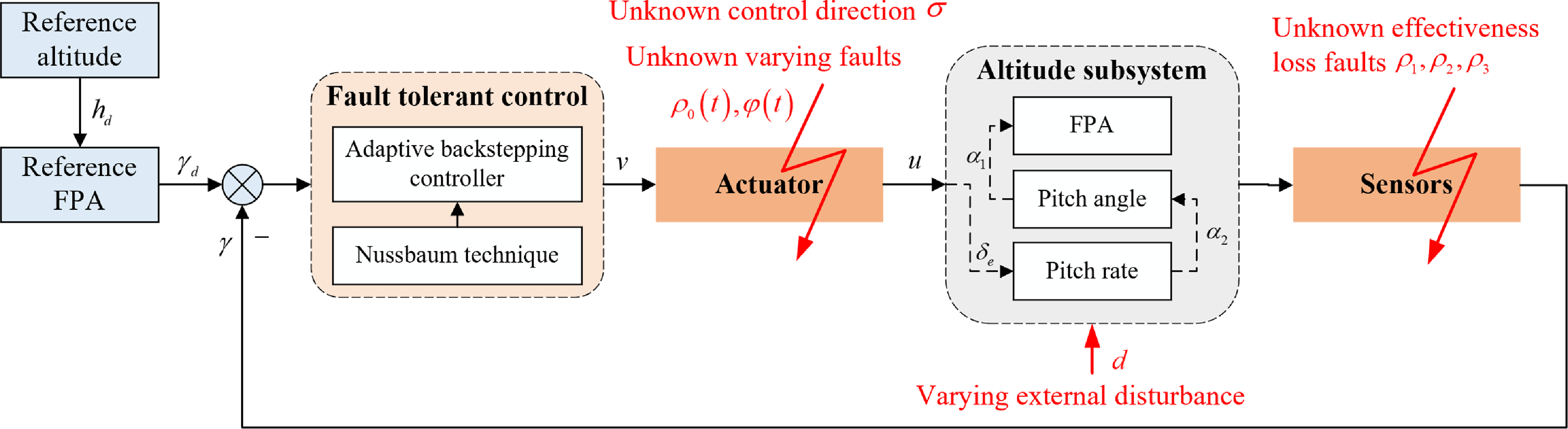
Figure 2. Structure diagram of proposed FTC design scheme.
Remark 3.4 Due to the unknown effectiveness loss faults of system sensors, the state variables cannot be obtained accurately. Therefore, the actual sensor measured values $x_i^F,{\rm{ i = 1,2,3}}$
are adopted in the backstepping controller design algorithm.
$x_i^F,{\rm{ i = 1,2,3}}$
are adopted in the backstepping controller design algorithm.
In the adaptive backstepping control strategy, the entire recursive design procedure can be divided into four steps. The first two steps involve designing the virtual control variables ${\alpha _1}$
and
${\alpha _1}$
and ${\alpha _2}$
, while Step 3 and Step 4 provide the final control law
${\alpha _2}$
, while Step 3 and Step 4 provide the final control law $v$
and associated adaptive law based on the Nussbaum function. The detailed design steps are presented below.
$v$
and associated adaptive law based on the Nussbaum function. The detailed design steps are presented below.
Step 1 In order for forcing $x_1^F$
to track the FPA command
$x_1^F$
to track the FPA command ${y_d}$
. Define the FPA tracking error
${y_d}$
. Define the FPA tracking error ${z_1}$
as
${z_1}$
as
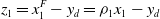 \begin{align}{z_1} = x_1^F - {y_d} = {\rho _1}{x_1} - {y_d}\end{align}
where ${y_d} = {\gamma _d}$
,
${y_d} = {\gamma _d}$
, $x_1^F$
denotes the measured value of
$x_1^F$
denotes the measured value of ${x_1}$
. The dynamics of
${x_1}$
. The dynamics of ${z_1}$
is written as
${z_1}$
is written as
 \begin{align}{\dot z_1} = \dot x_1^F - {\dot y_d} = {\rho _1}({f_1} + {g_1}{x_2}) - {\dot y_d}\end{align}
where ${\dot y_d} = {\dot \gamma _d}$
. The designed virtual control variable
${\dot y_d} = {\dot \gamma _d}$
. The designed virtual control variable ${\alpha _1}$
is introduced as
${\alpha _1}$
is introduced as
 \begin{align}{\alpha _1} = \frac{{ - {c_1}{z_1} - f_1^F + {{\dot y}_d}}}{{{g_1}}}\end{align}
where ${c_1} \gt 0$
is the gain parameter. According to the Assumption 2.3,
${c_1} \gt 0$
is the gain parameter. According to the Assumption 2.3, ${f_1}$
can be simplified to
${f_1}$
can be simplified to ${f_1} = {\varsigma _1}{x_1} + {\varsigma _2}$
. Thus,
${f_1} = {\varsigma _1}{x_1} + {\varsigma _2}$
. Thus, $f_1^F = {\varsigma _1}x_1^F + {\varsigma _2}$
. Similarly, aiming at forcing
$f_1^F = {\varsigma _1}x_1^F + {\varsigma _2}$
. Similarly, aiming at forcing ${\alpha _1}$
to track
${\alpha _1}$
to track $x_2^F$
, we define the error
$x_2^F$
, we define the error ${z_2}$
between
${z_2}$
between $x_2^F$
and
$x_2^F$
and ${\alpha _1}$
as
${\alpha _1}$
as
 \begin{align}{z_2} = x_2^F - {\alpha _1} = {\rho _2}{x_2} - {\alpha _1}\end{align}
And ${x_2}$
is obtained as
${x_2}$
is obtained as
 \begin{align}{x_2} = \frac{1}{{{\rho _2}}}\left( {{z_2} + {\alpha _1}} \right)\end{align}
Applying Equations (27)–(29) into Equation (26), ${\dot z_1}$
can be rewritten as
${\dot z_1}$
can be rewritten as
 \begin{align}{{\dot z}_1} &= {\rho _1}\left( {{f_1} + \frac{{{g_1}}}{{{\rho _2}}}\left( {{z_2} + {\alpha _1}} \right)} \right) - {{\dot y}_d} = {\rho _1}\left( {{f_1} + \frac{{{g_1}}}{{{\rho _2}}}\left( {{z_2} + \frac{{ - {c_1}{z_1} - f_1^F + {{\dot y}_d}}}{{{g_1}}}} \right)} \right) - {{\dot y}_d}\nonumber \\ & = \left({\rho _1}{f_1} - \frac{{{\rho _1}}}{{{\rho _2}}}f_1^F\right) + \frac{{{\rho _1}}}{{{\rho _2}}}({g_1}{z_2} - {c_1}{z_1} + {{\dot y}_d}) - {{\dot y}_d} \end{align}
Based on the FPA tracking error ${z_1}$
(Equation (25)), the first Lyapunov function is chosen as
${z_1}$
(Equation (25)), the first Lyapunov function is chosen as
 \begin{align}{V_1} = \frac{1}{2}z_1^2\end{align}
The derivative of ${V_1}$
can be given as
${V_1}$
can be given as
 \begin{align}{{\dot V}_1} &= {z_1}{{\dot z}_1} = {z_1}\left({\rho _1}{f_1} - \frac{{{\rho _1}}}{{{\rho _2}}}f_1^F\right) + \frac{{{\rho _1}}}{{{\rho _2}}}{z_1}({g_1}{z_2} - {c_1}{z_1} + {{\dot y}_d}) - {z_1}{{\dot y}_d}\nonumber \\ &= \left( {1 - \frac{{{\rho _1}}}{{{\rho _2}}}} \right){\varsigma _1}{z_1}\left( {{z_1} + {y_d}} \right) + \left( {{\rho _1} - \frac{{{\rho _1}}}{{{\rho _2}}}} \right){\varsigma _2}{z_1} + \frac{{{g_1}{\rho _1}}}{{{\rho _2}}}{z_1}{z_2} - {c_1}\frac{{{\rho _1}}}{{{\rho _2}}}z_1^2 + \left( {\frac{{{\rho _1}}}{{{\rho _2}}} - 1} \right){z_1}{{\dot y}_d}\end{align}
Step 2 The derivative of ${z_2}$
is
${z_2}$
is
 \begin{align}{\dot z_2} = \dot x_2^F - {\dot \alpha _1} = {\rho _2}{x_3} - {\dot \alpha _1}\end{align}
Based on the Assumption 2.2 and Assumption 2.3, ${\dot \alpha _1}$
is bounded as
${\dot \alpha _1}$
is bounded as
 \begin{align}{\dot \alpha _1} = \frac{{ - {c_1}{{\dot z}_1} - \dot f_1^F + {{\ddot y}_d}}}{{{g_1}}}\end{align}
where $\dot f_1^F = {\varsigma _1}\dot x_1^F$
. The virtual control
$\dot f_1^F = {\varsigma _1}\dot x_1^F$
. The virtual control ${\alpha _2}$
is designed as
${\alpha _2}$
is designed as
 \begin{align}{\alpha _2} = - {c_2}{z_2} + {\dot \alpha _1}\end{align}
where ${c_2} \gt 0$
is the gain parameter. To get
${c_2} \gt 0$
is the gain parameter. To get ${\alpha _2}$
to track
${\alpha _2}$
to track $x_3^F$
, the error
$x_3^F$
, the error ${z_3}$
is defined as
${z_3}$
is defined as
 \begin{align}{z_3} = x_3^F - {\alpha _2} = {\rho _3}{x_3} - {\alpha _2}\end{align}
Then ${x_3}$
can be rewritten as
${x_3}$
can be rewritten as
 \begin{align}{x_3} = \frac{1}{{{\rho _3}}}\left( {{z_3} + {\alpha _2}} \right)\end{align}
Based on the error ${z_2}$
(Equation (28)) the second Lyapunov function can be chosen as
${z_2}$
(Equation (28)) the second Lyapunov function can be chosen as
 \begin{align}{V_2} = \frac{1}{2}z_2^2\end{align}
Combining Equations (33)–(37) into Equation (38), the derivative of ${V_2}$
is given as
${V_2}$
is given as
 \begin{align}{{\dot V}_2}& = {z_2}{{\dot z}_2} = {z_2}\left( {\frac{{{\rho _2}}}{{{\rho _3}}}\left( {{z_3} - {c_2}{z_2} + {{\dot \alpha }_1}} \right) - {{\dot \alpha }_1}} \right) \nonumber \\ &= \frac{{{\rho _2}}}{{{\rho _3}}}{z_2}{z_3} - \frac{{{\rho _2}}}{{{\rho _3}}}{c_2}z_2^2 + {z_2}\left( {\frac{{{\rho _2}}}{{{\rho _3}}} - 1} \right)\left( {\frac{{ - {c_1}{{\dot z}_1} - \dot f_1^F + {{\ddot y}_d}}}{{{g_1}}}} \right)\end{align}
Step 3 The derivative of ${z_3}$
is
${z_3}$
is
 \begin{align}{\dot z_3} = \dot x_3^F - {\dot \alpha _2} = {\rho _3}\left( {{f_3} + {g_3}\left( {u + d} \right)} \right) - {\dot \alpha _2}\end{align}
where ${\dot \alpha _2}$
is bounded. Combining Equations (20), (34) and (35) into Equation (40), we can get the derivative of
${\dot \alpha _2}$
is bounded. Combining Equations (20), (34) and (35) into Equation (40), we can get the derivative of ${z_3}$
considering the actuator fault as
${z_3}$
considering the actuator fault as
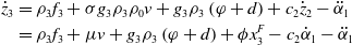 \begin{align}{{\dot z}_3} &= {\rho _3}{f_3} + \sigma {g_3}{\rho _3}{\rho _0}v + {g_3}{\rho _3}\left( {\varphi + d} \right) + {c_2}{{\dot z}_2} - {{\ddot \alpha }_1} \nonumber\\ &= {\rho _3}{f_3} + \mu v + {g_3}{\rho _3}\left( {\varphi + d} \right) + \phi x_3^F - {c_2}{{\dot \alpha }_1} - {{\ddot \alpha }_1}\end{align}
where $\mu = \sigma {g_3}{\rho _3}{\rho _0}$
,
$\mu = \sigma {g_3}{\rho _3}{\rho _0}$
, $\phi = {\rm{ }}{c_2}{\rho _2}/{\rho _3}$
are the unknown parameters for the simplification of subsequent controller design and system stability analysis.
$\phi = {\rm{ }}{c_2}{\rho _2}/{\rho _3}$
are the unknown parameters for the simplification of subsequent controller design and system stability analysis.
Based on the error ${z_3}$
(Equation (36)), we choose the third Lyapunov function as
${z_3}$
(Equation (36)), we choose the third Lyapunov function as
 \begin{align}{V_3} = \frac{1}{2}z_3^2\end{align}
Applying Equation (41) into Equation (42), the derivative of ${V_3}$
is given as
${V_3}$
is given as
 \begin{align}{\dot V_3} = {z_3}\left( {{\rho _3}{f_3} + \mu v + {g_3}{\rho _3}\left( {\varphi + d} \right) + \phi x_3^F} \right) + {\dot V^{\prime}_3}\end{align}
 \begin{align}{\dot V^{\prime}_3} = {z_3}\left( { - {c_2}{{\dot \alpha }_1} - {{\ddot \alpha }_1}} \right)\end{align}
Step 4 It can be noticed that the control gain $\mu $
is a variable including unknown parameters, so the Nussbaum function
$\mu $
is a variable including unknown parameters, so the Nussbaum function $N\left( k \right)$
is adopted, which is chosen as
$N\left( k \right)$
is adopted, which is chosen as $N\left( k \right) = {k^2}\cos \left( k \right)$
. The final control input is designed as follows
$N\left( k \right) = {k^2}\cos \left( k \right)$
. The final control input is designed as follows
 \begin{align}v = N\left( k \right)\bar v\end{align}
where
 \begin{align}\bar v = - {k_2}{z_3} - \beta \end{align}
 \begin{align}\beta = {k_1}{z_3} + \hat \phi x_3^F + \eta \tanh \left( {{z_3}} \right) + {\rho _3}f_3^F\end{align}
 \begin{align}\dot k = {\gamma _1}{z_3}\bar v\end{align}
where $\beta $
is the designed auxiliary variable.
$\beta $
is the designed auxiliary variable. $\hat \phi $
denotes the estimated value of
$\hat \phi $
denotes the estimated value of $\phi $
.
$\phi $
. $f_3^F$
is a function about the measured system state variables, which can be expressed as
$f_3^F$
is a function about the measured system state variables, which can be expressed as $f_3^F = \bar qS\bar c\big( {{C_m}\left( {x_2^F - x_1^F} \right) + {C_m}\left( {x_3^F} \right) - {c_e}\left( {x_2^F - x_1^F} \right)} \big)/{I_{yy}}$
.
$f_3^F = \bar qS\bar c\big( {{C_m}\left( {x_2^F - x_1^F} \right) + {C_m}\left( {x_3^F} \right) - {c_e}\left( {x_2^F - x_1^F} \right)} \big)/{I_{yy}}$
. ${k_1}$
,
${k_1}$
, ${k_2}$
and
${k_2}$
and ${\gamma _1}$
are the positive constants.
${\gamma _1}$
are the positive constants. $\eta $
is designed as
$\eta $
is designed as $\eta \geqslant \varepsilon + D$
where
$\eta \geqslant \varepsilon + D$
where $\varepsilon $
is a suitable positive constant.
$\varepsilon $
is a suitable positive constant. $\tanh ( \bullet )$
is a smooth hyperbolic tangent function that can be obtained from the hyperbolic sine function and the hyperbolic cosine function as
$\tanh ( \bullet )$
is a smooth hyperbolic tangent function that can be obtained from the hyperbolic sine function and the hyperbolic cosine function as $\tanh (x) = \sinh (x)/\cosh (x) = \left( {{e^x} - {e^{ - x}}} \right)/\left( {{e^x} + {e^{ - x}}} \right)$
, which can be employed in the control law to avoid the chattering problem in terms of eliminating varying external disturbance.
$\tanh (x) = \sinh (x)/\cosh (x) = \left( {{e^x} - {e^{ - x}}} \right)/\left( {{e^x} + {e^{ - x}}} \right)$
, which can be employed in the control law to avoid the chattering problem in terms of eliminating varying external disturbance.
The adaptive law of the estimated parameter $\hat \phi $
is designed as
$\hat \phi $
is designed as
 \begin{align}\dot {\hat \phi} = {\gamma _2}{z_3}x_3^F\end{align}
where ${\gamma _2}$
is the positive constant. In order for approximating the estimated value
${\gamma _2}$
is the positive constant. In order for approximating the estimated value $\hat \phi $
to the true value
$\hat \phi $
to the true value $\phi $
, we define the error
$\phi $
, we define the error $\tilde \phi = \hat \phi - \phi $
, and the fourth Lyapunov function is defined as
$\tilde \phi = \hat \phi - \phi $
, and the fourth Lyapunov function is defined as
 \begin{align}{V_4} = \frac{1}{{2{\gamma _2}}}{\tilde \phi ^2}\end{align}
And we can get $\dot {\tilde \phi} = \dot {\hat \phi} $
. The derivate of
$\dot {\tilde \phi} = \dot {\hat \phi} $
. The derivate of ${V_4}$
is given as
${V_4}$
is given as
 \begin{align}{\dot V_4} = \frac{1}{{{\gamma _2}}}{\tilde \phi} \dot {\hat \phi} = {z_3}\tilde \phi x_3^F \end{align}
Theorem 3.1 If Assumptions 2.1–2.5 are satisfied, considering HFV altitude subsystem (2)–(5) in the presence of the actuator and sensor’s faults (Equations (20)–(21)), unknown control direction and time-varying disturbance simultaneously, then utilising the designed control law (Equations (45)–(48)) and adaptive law (Equation (49)), all state variables of subsystem are uniformly ultimately bounded.
Proof On the basis of Equations (31), (38), (42) and (50), four Lyapunov functions are combined to obtain a new Lyapunov function as shown below, which is related to the errors ${z_1},{z_2},{z_3}\ {\rm{ and\ }}\tilde \phi $
 \begin{align}V = \sum\limits_{i = 1}^4 {{V_i}} = \frac{1}{2}z_1^2 + \frac{1}{2}z_2^2 + \frac{1}{2}z_3^2 + \frac{1}{{2{\gamma _2}}}{\tilde \phi ^2}\end{align}
Based on Assumption 2.4, and applying the Young’s inequality, Equations (32), (39) and (44) can be rewritten as follows
 \begin{align}{{\dot V}_1} &= \left( {1 - \frac{{{\rho _1}}}{{{\rho _2}}}} \right){\varsigma _1}{z_1}\left( {{z_1} + {y_d}} \right) + \left( {{\rho _1} - \frac{{{\rho _1}}}{{{\rho _2}}}} \right){\varsigma _2}{z_1} + \frac{{{g_1}{\rho _1}}}{{{\rho _2}}}{z_1}{z_2} - {c_1}\frac{{{\rho _1}}}{{{\rho _2}}}z_1^2 + \left( {\frac{{{\rho _1}}}{{{\rho _2}}} - 1} \right){z_1}{{\dot y}_d} \nonumber\\ &\le \left( {\varsigma _1^2 + \frac{{2 + {g_1}}}{{2{\rho _{20}}}} - {c_1}{\rho _{10}} + \frac{1}{2}} \right)z_1^2 + \left( {\frac{{{g_1}}}{{2{\rho _{20}}}}} \right)z_2^2 + \frac{1}{2}y_d^2 + \frac{1}{{2{\rho _{20}}}}\dot y_d^2 + \frac{1}{{2{\rho _{20}}}}\varsigma _2^2\end{align}
 \begin{align}{{\dot V}_2} &\le \frac{1}{{{\rho _{30}}}}\left( {\frac{{z_2^2}}{2} + \frac{{z_3^2}}{2}} \right) - {c_2}{\rho _{20}}z_2^2 + {z_2}\left( {\frac{{{\rho _2}}}{{{\rho _3}}} - 1} \right)\left( {\frac{1}{{{g_1}}}\left( { - {c_1}{{\dot z}_1} - {\varsigma _1}\left( {{{\dot z}_1} + {{\dot y}_d}} \right) + {{\ddot y}_d}} \right)} \right) \nonumber\\ &\le \frac{{1 + {c_1}}}{{2{g_1}}}\left( {1 - {c_1}{\rho _{10}}} \right)z_1^2 + \left( {\frac{1}{{2{\rho _{30}}}} + \frac{{1 + \varsigma _1^2}}{{2{g_1}}} + \frac{{1 + {c_1}}}{{2{\rho _{20}}}} + \frac{{\varsigma _1^2 + {c_1}}}{{{g_1}}}\left( {\varsigma _1^2 + \frac{{2 + {g_1}}}{{2{\rho _{20}}}} - \frac{{{c_1}{\rho _{10}}}}{2}} \right) - {c_2}{\rho _{20}}} \right)z_2^2 \nonumber\\ &+ \frac{1}{{2{\rho _{30}}}}z_3^2 + \frac{{1 + {c_1}}}{{2{g_1}}}y_d^2 + \left( {\frac{{1 + {c_1}}}{{2{g_1}{\rho _{20}}}} + \frac{1}{{2{g_1}}}} \right)\dot y_d^2 + \frac{1}{{2{g_1}}}\ddot y_d^2 + \frac{{1 + {c_1}}}{{2{g_1}{\rho _{20}}}}\varsigma _2^2 \end{align}
 \begin{align} {{\dot V^{\prime}}_3} &= {{{c_2}} \over {{g_1}}}\left( {{c_1} + {\varsigma _1}} \right){z_3}{{\dot z}_1} + {1 \over {{g_1}}}\left( {{c_1} + {\varsigma _1}} \right){z_3}{{\ddot z}_1} + {{{\varsigma _1}{c_2}} \over {{g_1}}}\left( {{z_3}{{\dot y}_d}} \right) - \left( {{c_2} + {{{\varsigma _1}} \over {{g_1}}}} \right){z_3}{{\ddot y}_d} - {1 \over {{g_1}}}{z_3}{{\dddot y}_d} \nonumber \\ &\le {{{c_1}{c_2}} \over {2{g_1}}}\left( {1 - {c_1}{\rho _{10}}} \right)z_1^2 + {{{c_1}{c_2}} \over {2{\rho _{20}}}}z_2^2 + \left( {{{{c_1}{c_2}} \over {{g_1}}}\left( {\varsigma _1^2 + {{2 + {g_1}} \over {2{\rho _{20}}}} - {{{c_1}{\rho _{10}}} \over 2}} \right) + {{{c_1} + 2{g_1}{c_1}} \over {2{g_1}{\rho _{30}}}} + {{{c_2}\varsigma _1^2 - {\varsigma _1} + 1} \over {2{g_1}}}} \right)z_3^2 \nonumber \\ &+ {{{c_1}{c_2}} \over {2{g_1}}}y_d^2 + \left( {{{{c_1}{c_2}} \over {2{g_1}{\rho _{20}}}} + {{{c_2}} \over {2{g_1}}}} \right)\dot y_d^2 + \left( {{{{c_1}} \over {2{g_1}{\rho _{30}}}} - {{{\varsigma _1}} \over {2{g_1}}}} \right)\ddot y_d^2 + {1 \over {2{g_1}}}\dddot y_d^2 + {{{c_1}{c_2}} \over {2{g_1}{\rho _{20}}}}\varsigma _2^2 \end{align}
The unknown effectiveness loss fault degrees of sensors have the properties as ${\rho _1}/{\rho _2} \geqslant {\rho _{10}}$
,
${\rho _1}/{\rho _2} \geqslant {\rho _{10}}$
, ${\rho _1}/{\rho _3} \geqslant {\rho _{10}}$
, and
${\rho _1}/{\rho _3} \geqslant {\rho _{10}}$
, and ${\rho _2}/{\rho _1} \geqslant {\rho _{20}}$
,
${\rho _2}/{\rho _1} \geqslant {\rho _{20}}$
, ${\rho _3}/{\rho _1} \geqslant {\rho _{30}}$
. Besides, there are
${\rho _3}/{\rho _1} \geqslant {\rho _{30}}$
. Besides, there are ${\rho _1}/{\rho _2} \le 1/{\rho _{20}}$
,
${\rho _1}/{\rho _2} \le 1/{\rho _{20}}$
, ${\rho _1}/{\rho _3} \le 1/{\rho _{30}}$
.
${\rho _1}/{\rho _3} \le 1/{\rho _{30}}$
.
Combining with Equations (43), (51)–(55), the derivate of $V$
can be rewritten as
$V$
can be rewritten as
 \begin{align}\dot V &= {{\dot V}_1} + {{\dot V}_2} + {{\dot V^{\prime}}_3} + {z_3}\left( {{\rho _3}{f_3} + \mu v + {g_3}{\rho _3}\left( {\varphi + d} \right) + \phi x_3^F} \right) + {{\dot V}_4} \nonumber\\& \le - {\Gamma _1}z_1^2 - {\Gamma _2}z_2^2 - {\Gamma _3}z_3^2 + {C_1} + {z_3}\left( {{\rho _3}{f_3} + \mu v + {g_3}{\rho _3}\left( {\varphi + d} \right) + \phi x_3^F} \right) + {z_3}\tilde \phi x_3^F\end{align}
where
 \begin{align}{\Gamma _1} = {c_1}{\rho _{10}} - \varsigma _1^2 - \frac{{2 + {g_1}}}{{2{\rho _{20}}}} - \frac{{{c_1}{c_2} + {c_1} + 1}}{{2{g_1}}}\left( {1 - {c_1}{\rho _{10}}} \right) - \frac{1}{2}\end{align}
 \begin{align}{\Gamma _2} = {c_2}{\rho _{20}} - \frac{1}{{2{\rho _{30}}}} - \frac{{1 + \varsigma _1^2}}{{2{g_1}}} - \frac{{\varsigma _1^2 + {c_1}}}{{{g_1}}}\left( {\varsigma _1^2 + \frac{{2 + {g_1}}}{{2{\rho _{20}}}} - \frac{{{c_1}{\rho _{10}}}}{2}} \right) - \frac{{{c_1}{c_2} + {c_1} + {g_1} + 1}}{{2{\rho _{20}}}}\end{align}
 \begin{align}{\Gamma _3} = - \frac{1}{{2{\rho _{30}}}} - \frac{{{c_1}{c_2}}}{{{g_1}}}\left( {\varsigma _1^2 + \frac{{2 + {g_1}}}{{2{\rho _{20}}}} - \frac{{{c_1}{\rho _{10}}}}{2}} \right) - \frac{{{c_1} + 2{g_1}{c_1}}}{{2{g_1}{\rho _{30}}}} - \frac{{{c_2}\varsigma _1^2 - {\varsigma _1} + 1}}{{2{g_1}}}\end{align}
 \begin{align} {C_1} = \left( { - {1 \over 2} - {{{c_1}{c_2} + {c_1} + 1} \over {2{g_1}}}} \right)y_d^2 + \left( { - {1 \over {2{\rho _{20}}}} - {{{c_1}{c_2} + {c_1} + 1} \over {2{g_1}{\rho _{20}}}} - {{{c_2} + 1} \over {2{g_1}}}} \right)\dot y_d^2 \nonumber \\ + \left( {{{{\varsigma _1} - 1} \over {2{g_1}}} - {{{c_1}} \over {2{g_1}{\rho _{30}}}}} \right)\ddot y_d^2 - {1 \over {2{g_1}}}\dddot y_d^2 + \left( { - {1 \over {2{\rho _{20}}}} - {{{c_1}{c_2} + {c_1} + 1} \over {2{g_1}{\rho _{20}}}}} \right)\varsigma _2^2 \end{align}
Based on Equations (13), (14) and (19), applying designed control law (Equations (45)–(48)) into Equation (56), $\dot V$
can be given as
$\dot V$
can be given as
 \begin{align}{\dot V} &\le - {\Gamma _1}z_1^2 - {\Gamma _2}z_2^2 - {\Gamma _3}z_3^2 + {z_3}\left( {\mu v + {g_3}{\rho _3}\left( {\varphi + d} \right) + {\rho _3}{f_3} + \phi x_3^F} \right) + \frac{1}{{{\gamma _2}}}{\tilde \phi} \dot {\hat \phi} + {C_1} \nonumber \\ &= - \sum\limits_{i = 1}^3 {{\Gamma _i}z_i^2} + {z_3}\left( {\beta - \left( {{k_1}{z_3} + \hat \phi x_3^F + \eta {\mathop{\rm sgn}} \left( {{z_3}} \right) + {\rho _3}f_3^F} \right) + \mu N\left( k \right)\bar v + {g_3}{\rho _3}\left( {\varphi + d} \right) + {\rho _3}{f_3} + \phi x_3^F} \right)\nonumber \\ &+ {z_3}\tilde \phi x_3^F - \frac{{\dot k}}{{{\gamma _1}}} + \frac{{\dot k}}{{{\gamma _1}}} + {C_1}\nonumber \\ &\le - \sum\limits_{i = 1}^3 {{\Gamma _i}z_i^2} + {z_3}\left( {\beta - {k_1}{z_3} + \tilde \phi x_3^F - \hat \phi x_3^F + \mu N\left( k \right)\bar v + \phi x_3^F} \right) + \frac{1}{2}z_3^2 - \frac{{\dot k}}{{{\gamma _1}}} + {z_3}\left( { - {k_2}{z_3} - \beta } \right) + {C_2}\nonumber \\ & \le - \sum\limits_{i = 1}^3 {{\Gamma _i}z_i^2} - \left( {{k_1} + {k_2} - \frac{1}{2}} \right)z_3^2 + \left( {\mu N\left( k \right) - 1} \right)\frac{{\dot k}}{{{\gamma _1}}} + {C_2}\nonumber \\ &\le - \lambda V + \left( {\mu N\left( k \right) - 1} \right)\frac{{\dot k}}{{{\gamma _1}}} + {C_2}\end{align}
where $\left| {{\rho _3}\left( {{f_3} - f_3^F} \right)} \right| \le \bar \omega $
,
$\left| {{\rho _3}\left( {{f_3} - f_3^F} \right)} \right| \le \bar \omega $
, ${C_2} = {C_1} + {\bar \omega ^2}/2$
,
${C_2} = {C_1} + {\bar \omega ^2}/2$
, $\lambda = \min \left\{ {{\Gamma _1},{\Gamma _2},{\Gamma _3} + {k_1} + {k_2} - 1/2} \right\} \gt 0$
. Multiplying by
$\lambda = \min \left\{ {{\Gamma _1},{\Gamma _2},{\Gamma _3} + {k_1} + {k_2} - 1/2} \right\} \gt 0$
. Multiplying by ${e^{\lambda t}}$
and integrating it, we have
${e^{\lambda t}}$
and integrating it, we have
 \begin{align}V\left( t \right) &\le \left( {V\left( 0 \right) - \frac{{{C_2}}}{\lambda }} \right){e^{ - \lambda t}} + \frac{{{C_2}}}{\lambda } + \frac{{{e^{ - \lambda t}}}}{{{\gamma _1}}}\int_0^t {\left( {\mu N\left( k \right) - 1} \right)\dot k{e^{\lambda \tau }}d\tau } \nonumber \\ &\le \left| {V\left( 0 \right) - \frac{{{C_2}}}{\lambda }} \right| + \left| {\frac{{{C_2}}}{\lambda }} \right| + \frac{{{e^{ - \lambda t}}}}{{{\gamma _1}}}\int_0^t {\left( {\mu N\left( k \right) - 1} \right)\dot k{e^{\lambda \tau }}d\tau } \nonumber \\ &= \xi + \frac{{{e^{ - \lambda t}}}}{{{\gamma _1}}}\int_0^t {\left( {\mu N\left( k \right) - 1} \right)\dot k{e^{\lambda \tau }}d\tau } \end{align}
where $\xi = \left| {V\left( 0 \right) - \frac{{{C_2}}}{\lambda }} \right| + \left| {\frac{{{C_2}}}{\lambda }} \right|$
. According to Lemma 2.1, we can obtain that
$\xi = \left| {V\left( 0 \right) - \frac{{{C_2}}}{\lambda }} \right| + \left| {\frac{{{C_2}}}{\lambda }} \right|$
. According to Lemma 2.1, we can obtain that $V\left( t \right)$
is bounded on
$V\left( t \right)$
is bounded on $[0,{t_f})$
, which means the tracking errors
$[0,{t_f})$
, which means the tracking errors ${z_1},{z_2},{z_3}$
and estimated error
${z_1},{z_2},{z_3}$
and estimated error $\tilde \phi $
have upper bounds. Therefore, with the appropriate parameters designed, the proposed controller can guarantee that all state variables of the HFV altitude subsystem are ultimately bounded stable considering the unknown actuator and sensor faults, unknown control direction and varying external disturbance.
$\tilde \phi $
have upper bounds. Therefore, with the appropriate parameters designed, the proposed controller can guarantee that all state variables of the HFV altitude subsystem are ultimately bounded stable considering the unknown actuator and sensor faults, unknown control direction and varying external disturbance.
4.0 Simulation
In this section, the effectiveness of the proposed controller is verified through numerical simulations. The flight environment and initial state variables are set as $h = 110000\,{\rm{ ft}}$
,
$h = 110000\,{\rm{ ft}}$
, $V = 15060{\rm{ ft/s}}$
,
$V = 15060{\rm{ ft/s}}$
, ${\gamma _0} = 0{\rm{ rad}}$
,
${\gamma _0} = 0{\rm{ rad}}$
, ${\theta _0} = 0.0315{\rm{ rad}}$
,
${\theta _0} = 0.0315{\rm{ rad}}$
, ${q_0} = 0{\rm{ rad/s}}$
. The time-varying external disturbance is chosen as
${q_0} = 0{\rm{ rad/s}}$
. The time-varying external disturbance is chosen as $d = 0.02 + 0.01\sin \left( t \right)$
. In the whole process of simulation, the reference altitude command is
$d = 0.02 + 0.01\sin \left( t \right)$
. In the whole process of simulation, the reference altitude command is $112000\,{\rm{ ft}}$
in first
$112000\,{\rm{ ft}}$
in first $50{\rm{ s}}$
and will be switched back to initial altitude
$50{\rm{ s}}$
and will be switched back to initial altitude $110000\,{\rm{ ft}}$
as follows:
$110000\,{\rm{ ft}}$
as follows:
 \begin{align}{h_d} = \left\{ {\begin{array}{*{20}{l}}{112000\,{\rm{ ft, \quad if\ 0\ s}} \le t{\rm{ \lt 50\ s}}}\\{110000\,{\rm{ ft,\quad if\ 50\ s}} \le t \le {\rm{100\ s }}}\end{array}} \right.\end{align}
To avoid a differential explosion in the step response, the desired altitude command ${h_{df}}$
is generated from the output of the following two-order filter.
${h_{df}}$
is generated from the output of the following two-order filter.
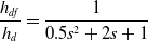 \begin{align}\frac{{{h_{df}}}}{{{h_d}}} = \frac{1}{{0.5{s^2} + 2s + 1}}\end{align}
The FPA command parameters are set as ${k_h} = 0.5$
,
${k_h} = 0.5$
, ${k_i} = 0.1$
. The controller gain parameters and adaptive law parameters are selected as
${k_i} = 0.1$
. The controller gain parameters and adaptive law parameters are selected as ${c_1} = 6$
,
${c_1} = 6$
, ${c_2} = 1$
,
${c_2} = 1$
, ${k_1} = 8$
,
${k_1} = 8$
, ${k_2} = 9$
,
${k_2} = 9$
, ${\gamma _1} = 20$
,
${\gamma _1} = 20$
, ${\gamma _2} = 1$
. And the robust term parameter is chosen as
${\gamma _2} = 1$
. And the robust term parameter is chosen as $\varepsilon = 0.1$
. To demonstrate the effectiveness of the proposed controller, we take PID controller with their gain parameters set to
$\varepsilon = 0.1$
. To demonstrate the effectiveness of the proposed controller, we take PID controller with their gain parameters set to $[300,40,500]$
as the comparison.
$[300,40,500]$
as the comparison.
For more comprehensive fault types analysis of actuator and sensors, we simulate the following cases:
-
(1) In Case 1, we assume that the fault types of actuator and sensors both are fixed, that is, the values of fault degrees are constants. For sensors, the effectiveness loss fault degrees are considered as
${\rho _1} = 0.8$
,
${\rho _2} = 0.9$
,
${\rho _3} = 0.7$
. For actuator, the control direction is set as a positive constant
$\sigma = 0.65$
, the effectiveness loss fault degree is set as
${\rho _0} = 0.5$
, and the bias fault degree is chosen as
$\varphi = 0.3$
. -
(2) In Case 2, to better simulate the change of actuator fatigue degree during a real hypersonic flight, the time-varying effectiveness loss fault type of actuator is introduced. Keeping all conditions unchanged, the different actuator effectiveness loss fault degrees are selected in different time periods as follows


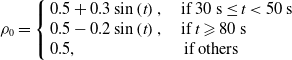 \begin{equation}{\rho _0} = \left\{ \begin{array}{l}0.5 + 0.3\sin \left( t \right),\quad{\rm{ if\ 30\ s }} \le {\rm{ }}t \lt 50\ {\rm{ s}}\\0.5 - 0.2\sin \left( t \right),\quad{\rm{ if\ }}t \geqslant 80\ {\rm{ s}}\\0.5,\qquad\qquad\qquad\,\,{\rm{ if\ others}}\end{array} \right.\end{equation}
-
(3) In Case 3, we assume that the degree of actuator bias fault is changeable, which considers the potential impacts of the harsh and volatile external environment on actuator stuck. The varying bias fault is more likely to occur in the hypersonic flight phase. Therefore, with the remaining conditions in Case 2 unchanged, the bias fault of actuator is given as
(66)
\begin{equation}\varphi = \left\{ \begin{array}{l}0.3 - 0.4\cos \left( t \right),\quad{\rm{ if\ 30\ s }} \le {\rm{ }}t \lt 50\ {\rm{ s}}\\0.3 + 0.6\cos \left( t \right),\quad{\rm{ if\ }}t \geqslant 80\ {\rm{ s}}\\0.3,\qquad\qquad\qquad\,\,{\rm{ if\ others}}\end{array} \right.\end{equation}
-
(4) In Case 4, we simulate the opposite signs of the unknown control direction, which is set to
$\sigma = - 5$
while keeping all other conditions unchanged from Case 3.


The simulation results of the above cases are shown in Figs. 3–15.
As shown in Fig. 3, which presents simulations of the fixed fault type of actuator and sensors in Case 1. The proposed controller has the basic fault-tolerant characteristic to track the reference altitude command including both climbing and descending stages within $14{\rm{s}}$
. Figs 4–7 show the altitude tracking comparison between the proposed FTC approach and the PID controller under Cases 2, 3 and 4. It can be clearly seen that the fluctuation of the proposed controller is significantly smaller than that of the PID controller, particularly when the actuator’s gain fault or bias fault degree varies with the changing flight environment. Furthermore, when control direction changes to a negative value in Case 4, the tracking control is still effective and stable under the proposed controller, while it fails under the PID controller. In Figs. 8–12, we can see that the state variables of altitude subsystem are uniformly bounded and stable with the proposed controller, but violent oscillation with PID control. The control input of the system in the presence of unknown faults of actuator and sensors, unknown control direction and external disturbance are provided in Figs 13–15. With the proposed controller, the varying faults and tracking commands lead to minor fluctuations of input at
$14{\rm{s}}$
. Figs 4–7 show the altitude tracking comparison between the proposed FTC approach and the PID controller under Cases 2, 3 and 4. It can be clearly seen that the fluctuation of the proposed controller is significantly smaller than that of the PID controller, particularly when the actuator’s gain fault or bias fault degree varies with the changing flight environment. Furthermore, when control direction changes to a negative value in Case 4, the tracking control is still effective and stable under the proposed controller, while it fails under the PID controller. In Figs. 8–12, we can see that the state variables of altitude subsystem are uniformly bounded and stable with the proposed controller, but violent oscillation with PID control. The control input of the system in the presence of unknown faults of actuator and sensors, unknown control direction and external disturbance are provided in Figs 13–15. With the proposed controller, the varying faults and tracking commands lead to minor fluctuations of input at $30{\rm{ s}}$
,
$30{\rm{ s}}$
, $50{\rm{ s}}$
and
$50{\rm{ s}}$
and $80{\rm{ s}}$
. Moreover, the control input is smaller and more practical compared to the PID controller in the actual hypersonic flight.
$80{\rm{ s}}$
. Moreover, the control input is smaller and more practical compared to the PID controller in the actual hypersonic flight.
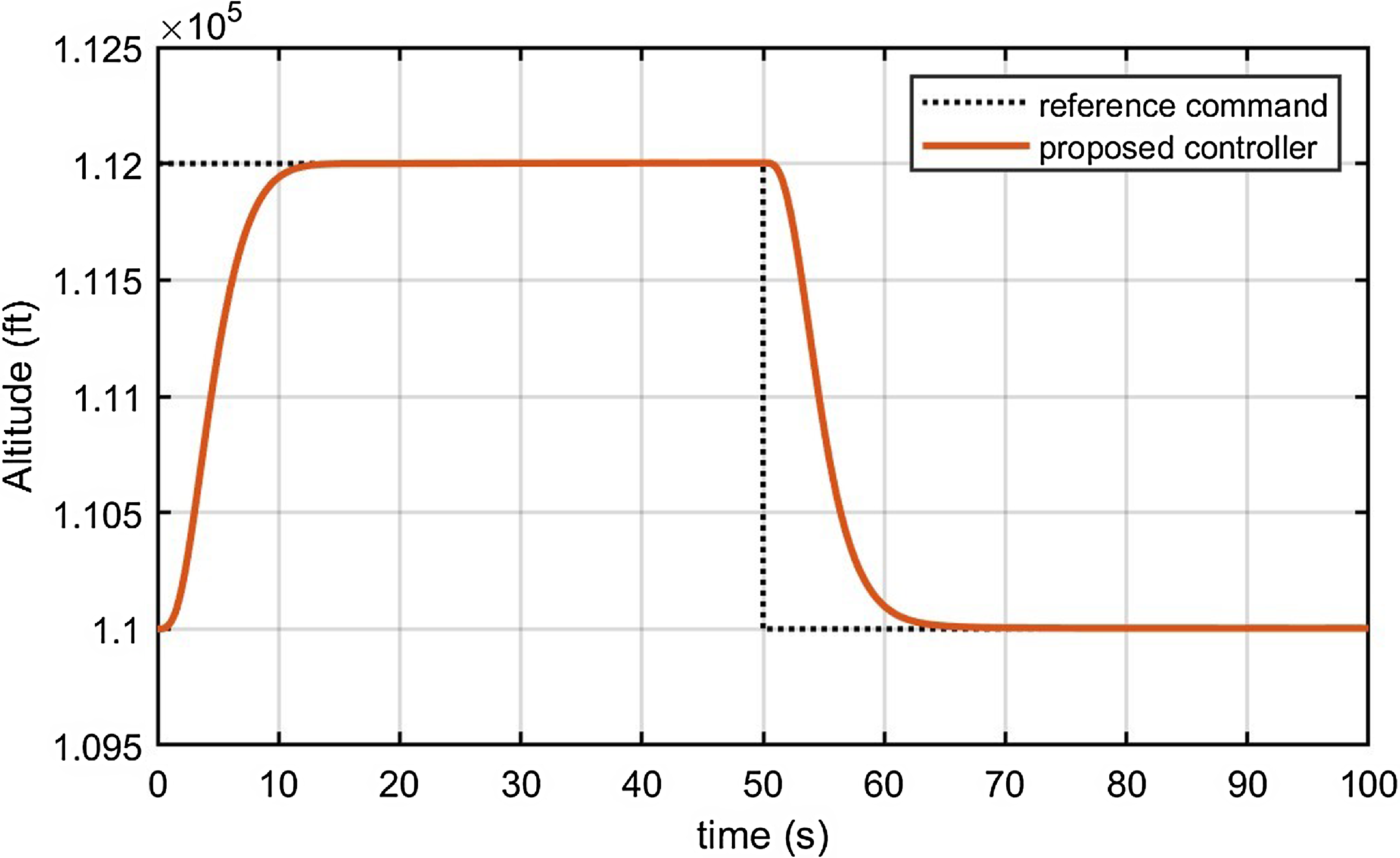
Figure 3. Altitude tracking response in Case 1.
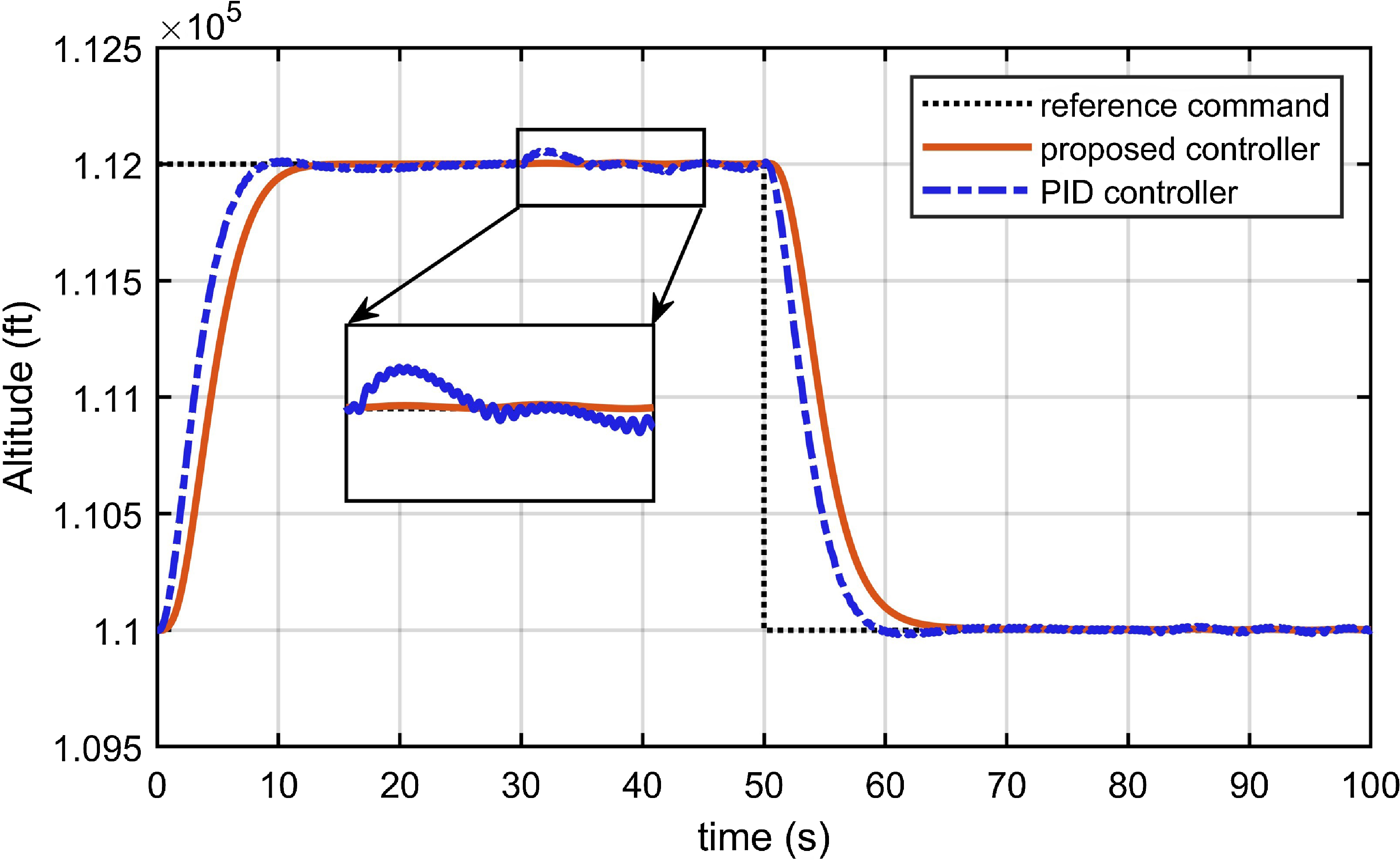
Figure 4. Altitude tracking response with the PID controller in Case 2.
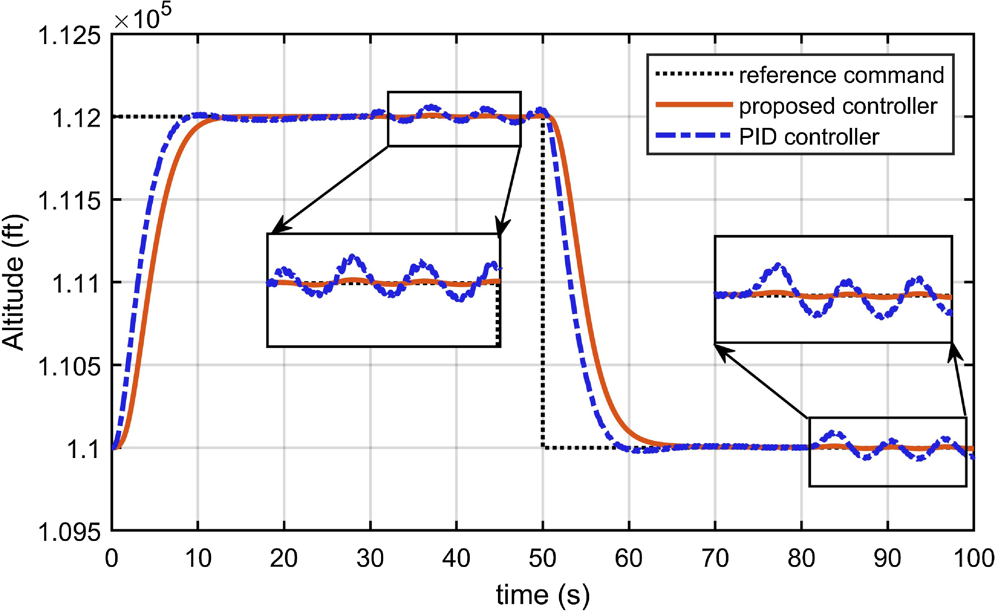
Figure 5. Altitude tracking response with the PID controller in Case 3.

Figure 6. Altitude tracking response in Case 4.
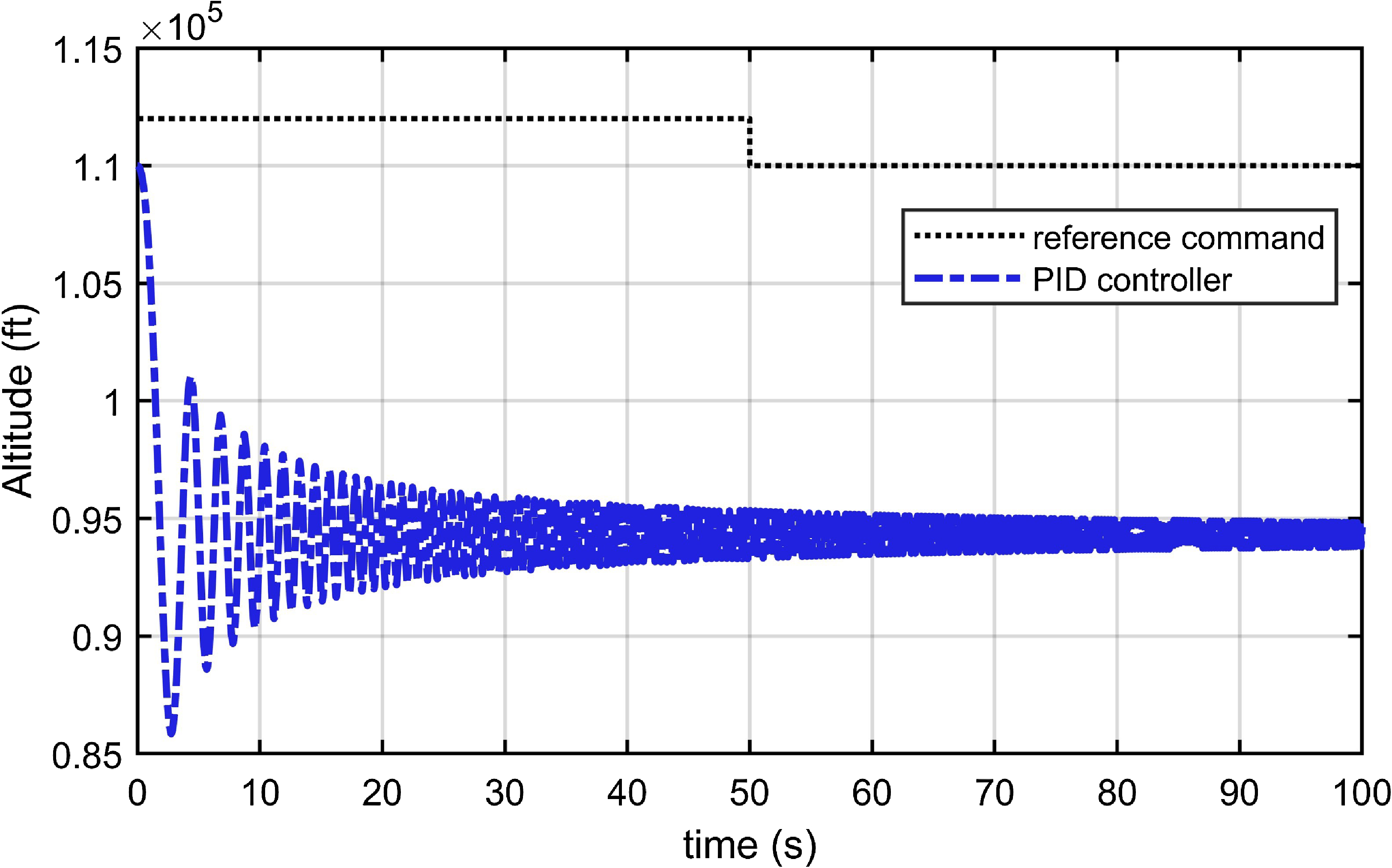
Figure 7. Altitude tracking response of the PID controller in Case 4.
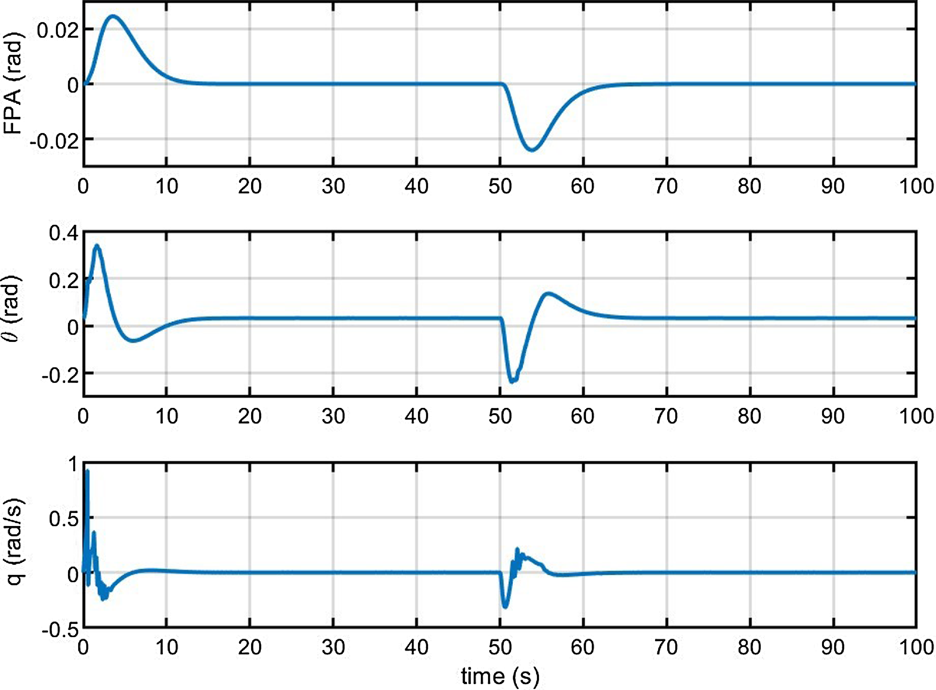
Figure 8. System state variables in Case 1.
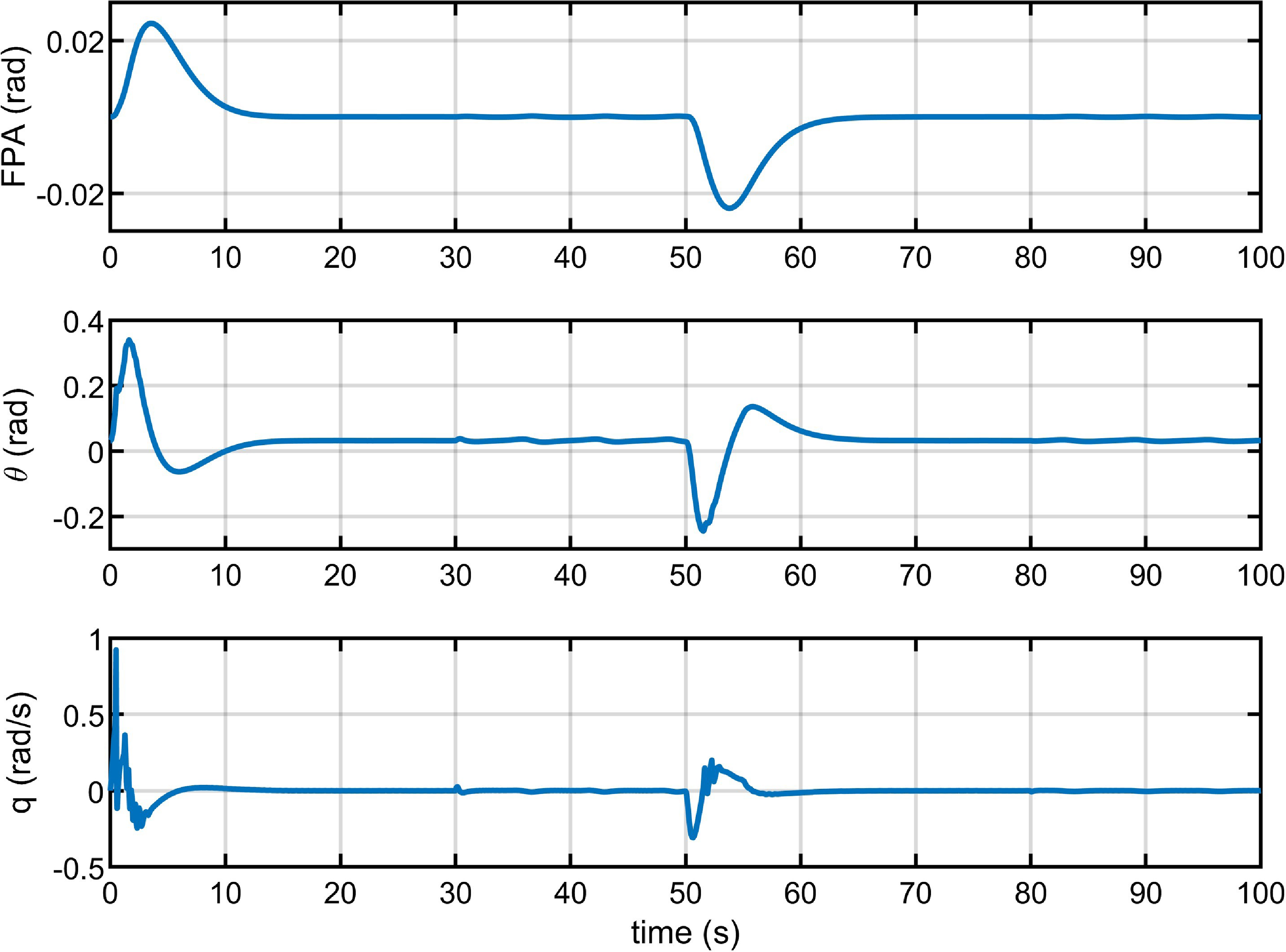
Figure 9. System state variables in Case 2.
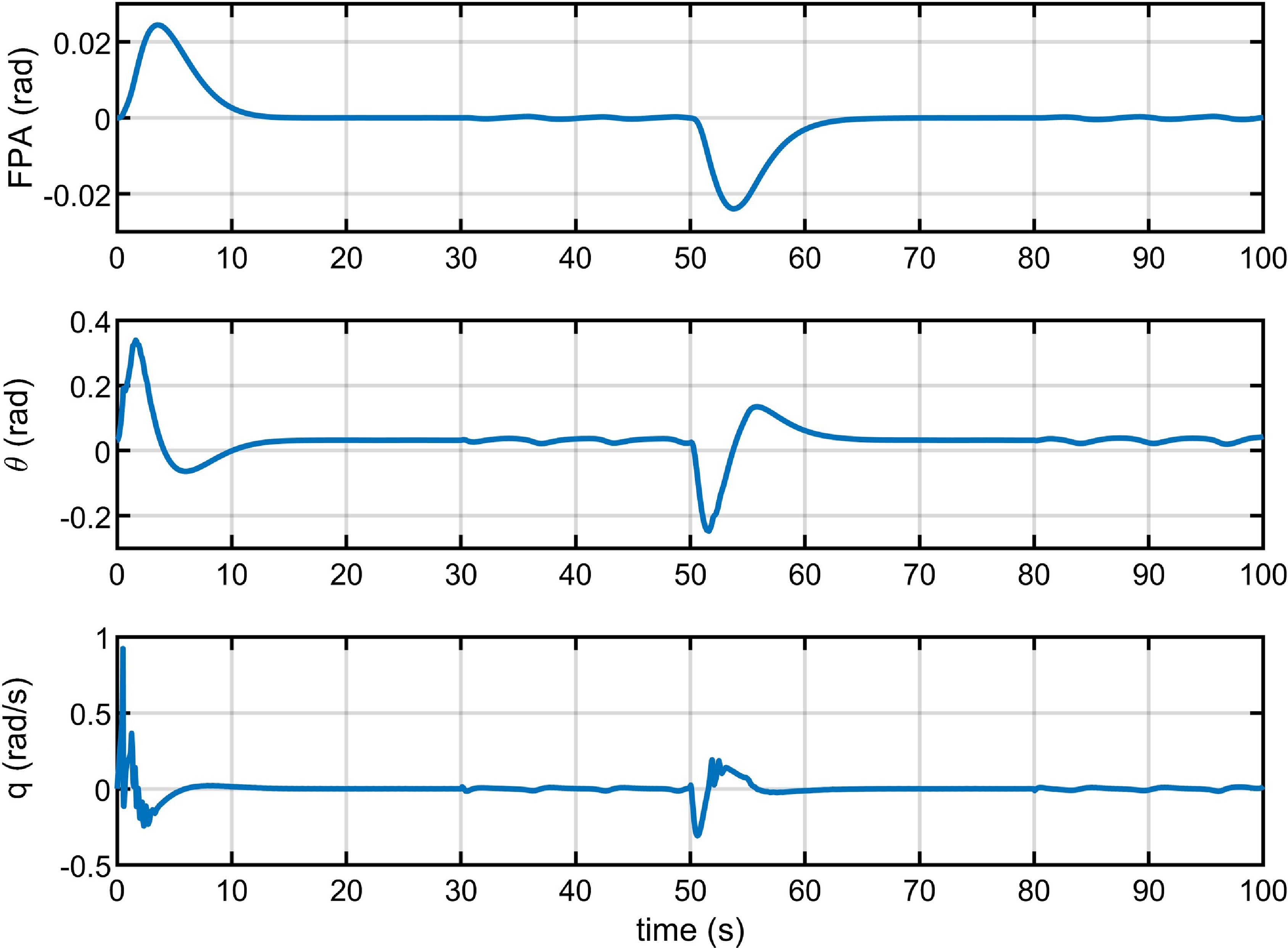
Figure 10. System state variables in Case 3.

Figure 11. System state variables of the PID controller in Case 3.
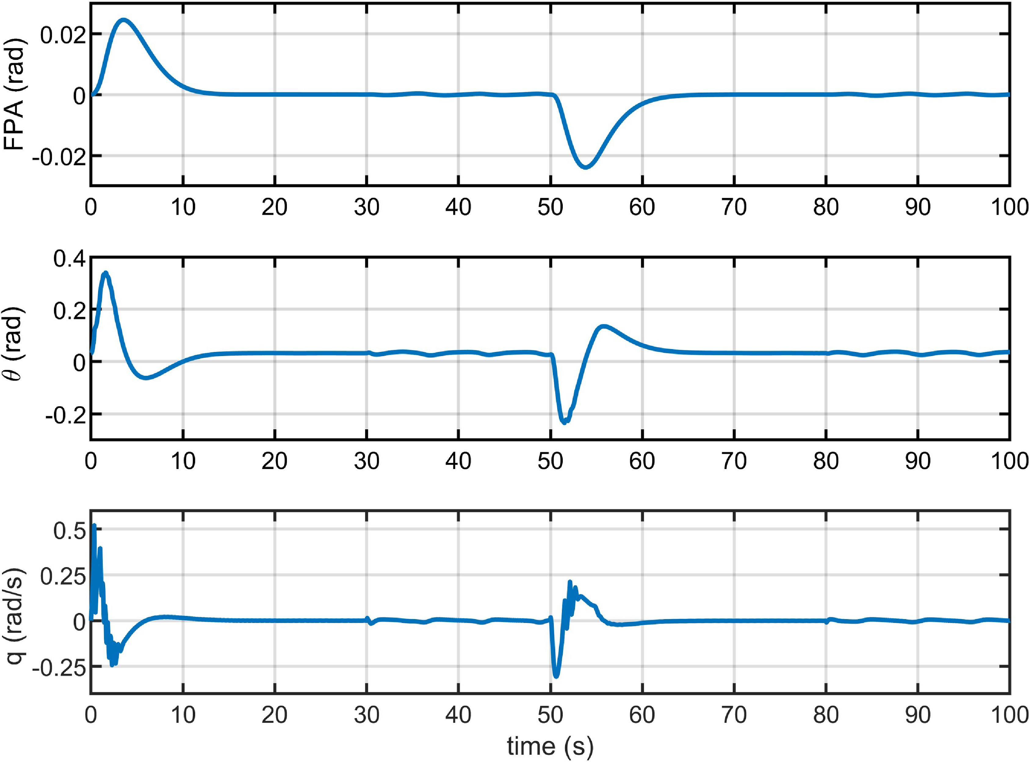
Figure 12. System state variables in Case 4.

Figure 13. Elevator deflection in Case 3.
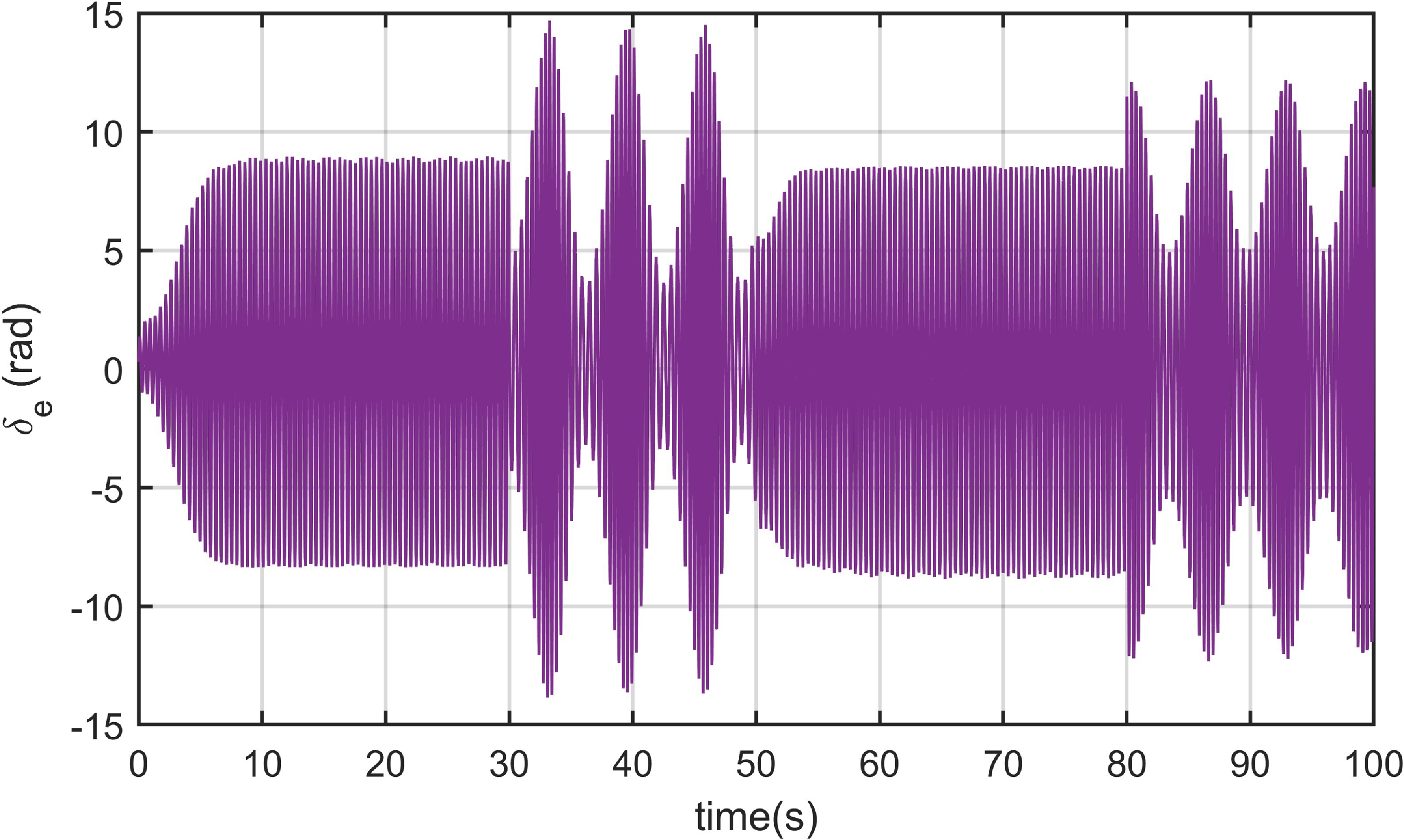
Figure 14. Elevator deflection of PID controller in Case 3.
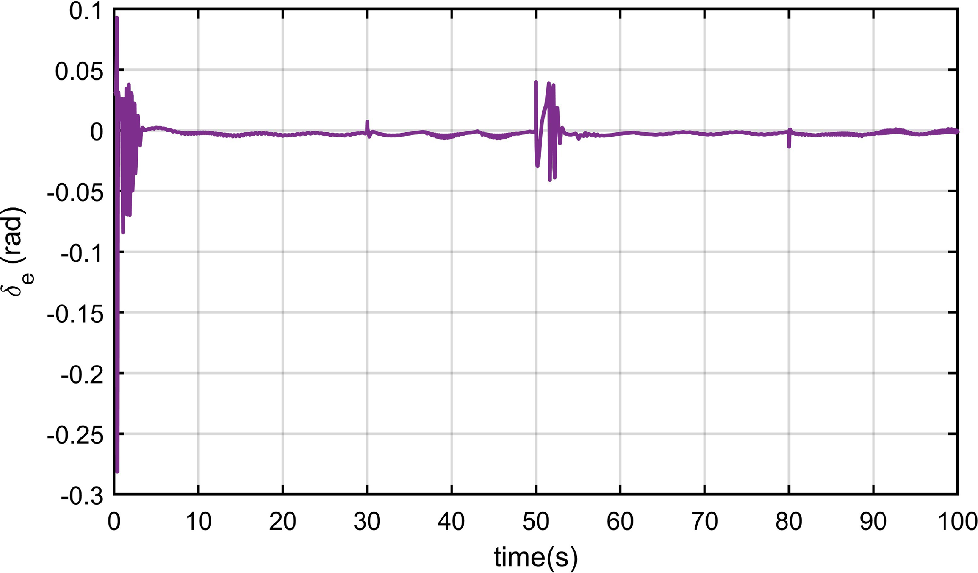
Figure 15. Elevator deflection in Case 4.
Under the various conditions of component faults and varying disturbance, which specifically consider the common fault types of the actuator and sensors during the hypersonic flight, these simulation results demonstrate that the proposed controller has the better control performance, including reliable robustness and stronger stability in comparison with the PID control method. Notably, the proposed control strategy effectively suppresses the fluctuations caused by unknown faults of actuator and sensors under varying external disturbance. Furthermore, it successfully addresses the issue of unknown control direction of the actuator.
5.0 Conclusion
This study focuses on the controller design for the HFV system that can effectively handle the problems of simultaneous actuator and sensor faults and unknown control direction under varying external disturbance, which can provide a new idea for the FTC method of HFV in future. Based on the dynamics modelling, analysis and design of various fault types, a novel adaptive backstepping FTC algorithm with auxiliary variables design based on the Nussbaum gain function technique is proposed, which can ensure the stable control of the system considering unknown varying fault parameters and possible control direction singularity. The detailed process of proving the closed-loop system stability is given based on the Lyapunov method. The effectiveness and superiority of the proposed controller are validated through different fault cases of actuator and sensors in numerical simulations with the PID controllers compared.
Acknowledgements
This research did not receive any specific grant from funding agencies in the public, commercial, or not-for-profit sectors.
Competing interests
The authors declare none.


