


1. Introduction
Raindrops are absorbed by wet soil, tea can rise within a biscuit dipped in a cup and a sponge swells when soaking up water. These common phenomena all involve capillary imbibition into a porous structure (Ha & Kim Reference Ha and Kim2020). A porous material is often considered as an assembly of individual capillary channels (or tubes) in which the progression of a fluid is captured by Darcy's law linking the pressure gradient to the fluid velocity. In a capillary tube, a wetting fluid will form a curved meniscus, leading to a constant negative capillary pressure sucking the fluid into the tube. This suction fights a growing viscous drag due to the presence of the tube boundaries, leading to a gradual slowing down of the fluid. In the early 20th century, Lucas (Reference Lucas1918), Bell & Cameron (Reference Bell and Cameron1906) and Washburn (Reference Washburn1921) showed that, in the absence of gravity, the position of the meniscus  $z_m(t)$ scales as $\sqrt {t}$. In the case of a sponge, and more generally swellable porous materials, the microscopic porous structure is composed of cellulose, a material that swells when exposed to water (Kvick et al. Reference Kvick, Martinez, Hewitt and Balmforth2017). Swelling occurs when solvent molecules penetrate a polymeric network, leading to its elastic deformation. It is observed for most natural fibres exposed to water (e.g. cellulose, hemp or flax; see Pucci, Liotier & Drapier Reference Pucci, Liotier and Drapier2016; Testoni et al. Reference Testoni, Kim, Pisupati and Park2018). The absorption of fluid leads to a change in geometry at the macroscopic scale and often to large-scale motions or deformations. For example, a paper sheet will spontaneously curl when placed upon a bath of water (Reyssat & Mahadevan Reference Reyssat and Mahadevan2011), while the petals of a pine cone will open or close depending on the ambient humidity (Reyssat & Mahadevan Reference Reyssat and Mahadevan2009). In the case of a sponge, the macroscopic pores change in size and distribution when the cellulose matrix swells. This modification in pore size affects the imbibition dynamics into the material. Similarly, it has been shown that, for fluids of equivalent viscosity and wettability, swelling slows down the capillary imbibition of fluids in paper sheets (Kim & Mahadevan Reference Kim and Mahadevan2006). Several mechanisms for this slowing down have been given, depending on the density of the fibres. The pore sizes might either grow or shrink, depending on the mobility of the fibres (Schuchardtl Reference Schuchardtl1991; Takahashi, Häggkvist & Li Reference Takahashi, Häggkvist and Li1997; Chang & Kim Reference Chang and Kim2020; Duprat Reference Duprat2022).
The examples of paper and sponges show the complexity of the coupled swelling–imbibition problem. Justifications of the different models rely on experimental observations at the scale of the paper sheet or the sponge. Simultaneously observing both the fluid progression and the swelling of the matrix is complex. Model experiments on single swelling pores could help us to understand the physical principles underlying these problems. Several studies have described the imbibition into capillary tubes made of hydrogels (Chang, Jensen & Kim Reference Chang, Jensen and Kim2022), but the behaviour of individual pores of swellable fibrous materials remains elusive.
In this paper, we describe the imbibition of fluid between two stretched and parallel fibres made of a swelling elastomer of well-known properties. The model pore formed by the fibres has the advantage of allowing easy visualization of both the fluid front and the swelling of the material. Moreover, this system also allows us to examine the effect of stresses within the material, which impact both the swelling properties and the overall deformations of the material. We show that, for swelling fibres, imbibition becomes possible for larger distances than in the non-swelling case. We describe the dynamics of this imbibition and show the existence of a swelling-dominated imbibition at constant velocity. Our observations are compared with a linear poro-elastic theory capturing the main physical ingredients of our problem and highlighting in return the change in the material's elastic properties. Finally, we describe the elasto-capillary collapse of our model pore, which can be observed once surface tension forces overcome the restoring tension force within the fibres.
2. Imbibition between two swellable fibres
2.1. Problem formulation and experimental set-up
We consider an elementary pore composed of two identical parallel fibres placed at a distance  $2d$ (figure 1a). The fibres, of initial unstretched length $L_0$ and radius $R_0$, are stretched to a length $L$. The stretching causes the fibre radius to decrease. In all that follows, $R(z,t)$ denotes the local radius of the fibres in the stretched state. In the case of rigid non-swelling fibres, $L = L_0$ and $R=R_0$ for all times and positions. In the case of swelling fibres, $R$ depends on both $z$ and $t$. The position of the meniscus is denoted $z_m$. In all that follows, the subscript ‘m’ refers to the fluid meniscus.

Figure 1. Experimental set-up and notations. Panel (a) (constant length) shows two fibres of initial radius  $R_0$ that are stretched to a length $L$ (held constant). The meniscus position is called $z_m$. Here, $d$ denotes the half-distance between the outer edges of the fibres. The fibres are clamped to a supporting frame at $z = 0$ and $z = L$ and held horizontally. A small portion of the fibres (approximately 2 mm) is in contact with the bath at $t = 0$. As the fibres swell, the fluid can progress in the model pore thanks to capillarity. Pictures are then taken from the top. Panel (b) (constant tension) shows that, to perform the experiment at constant tension, the fibres are attached to a mass $m$ and free to slide at $z = L$. The same supporting frame ensures that the fibres stay parallel and horizontal. The length is no longer constant.
To examine the effect of fibre swelling on the imbibition velocity, we fabricate fibres out of polyvinylsiloxane (PVS, Zhermack Elite Double 32), a silicon-based elastomer that swells when placed in contact with low-viscosity silicone oil. The fibres are fabricated by sucking degassed liquid PVS into capillary tubes of known inner radii (250, 400 and  $600\pm 1\,\mathrm {\mu }$m) before it becomes solid. After polymerizing, the elastic fibres are extracted by breaking the capillary tube and gently pulling on one end of the fibres. No preliminary treatment is done to the capillary tubes. We obtain fibres of Young's modulus $E = 0.9 \pm 0.1$ MPa and elastic Poisson ratio $\nu _P = \frac {1}{2}$. To describe the extent to which a fibre swells, we define the maximal swelling ratio of our fibres as
 \begin{equation} \lambda_{max} = \frac{R_{max}}{R_s}. \end{equation}
For an isotropically swelling material, it is defined so that  $\lambda _{max}^3 = {V_{swollen}}/{V_0}$, where $V_{swollen}$ is the volume of a polymer slab swollen completely under no mechanical constraints when immersed in a solvent bath and $V_0$ is its initial unswollen volume. We can also define the current swelling ratio (which will vary along the position of the fibre) as $\lambda (z,t) = {R(z,t)}/{R_s}$. In our case, $\lambda _{max} = 1.55 \pm 0.05$. The exact value of the maximal swollen radius depends slightly on the temperature as well as the tension applied to the fibres (Van de Velde et al. Reference Van de Velde, Dervaux, Protière and Duprat2022). The variations remain small compared with the overall swelling and we thus consider $\lambda _{max} = 1.55$, which was measured on free swelling fibres immersed in a solvent bath, to be a good approximation for our experiments. The swelling time scales depend highly on the fibre geometry and oil viscosity and can range anywhere from seconds to multiple days for large enough polymer blocks. More details on the time scales are discussed in § 3. Figure 1 presents the experimental set-up used throughout this study. Depending on the experiment, we used two different configurations. In configuration A (figure 1a), the fibres are prestretched and attached to a custom Plexiglas frame with engraved slits ensuring that the fibres stay parallel throughout the experiment. The total stretched length of the fibre is set to $L = 3$ cm (i.e. the length of the frame) unless otherwise specified. Calling $L_0$ the unstretched length of the fibres, the imposed stretch is given by $\epsilon = {L}/{L_0}-1$. At both ends, the fibres are clamped, ensuring that their length remains constant. As the fibre radius will shrink due to the stretch, we call $R_s = {R_0}/{\sqrt {1+\epsilon }}$ the radius of the fibre in its stretched state before any swelling. As the fibres are compressed at their ends due to the clamps, a small region (of the order of $1$ mm) is not perfectly circular. Nonetheless, as this portion is small compared with the fibre length, we assume that, before any swelling occurs, $R = R_s$ at all positions. The fibres are maintained horizontal during the whole experiment to prevent any gravitational effects. Before every experiment, any dust particles are removed using compressed air and any electrostatic charges are removed using an ion gun. An overfilled bath of low-viscosity silicone oil (Carl Roth, M2, M3 or M5, viscosity $\eta = 2.3$, $3.2$ or $5.4\pm 0.3$ mPa s) is then placed in contact with one end of the fibres (figure 1). A small portion of the fibres (approximately 2 mm) is thus always in contact with the oil. In the second configuration (figure 1b), the fibre length is no longer constant. It is still clamped at $z = 0$ where the fibres touch the oil bath but the fibres are able to slide within the slits of the supporting frame at $z = L$. As shown in the schematic, both fibres sit on a ballbearing and are connected to a known mass $m$ applying a constant tension on the fibres throughout the experiment. Unless otherwise specified, all presented experiments are performed at a constant length.
We track the evolution of the system by taking pictures at regular intervals using a camera (Basler ac 3.0) and a 50 mm lens. The frame rate is adjusted depending on the experiment. An image taken before the start of the experiment allows us to measure the values of  $d$ and $R_s$ before starting the imbibition. As the fibres are elongated objects and filmed as a whole, the resolution in the direction perpendicular to the flow is limited. One pixel corresponds to approximately 4 $\mathrm {\mu }$m in our measurements, which explains the uncertainty when measuring $d/R$.
2.2. Imbibition without swelling
The imbibition between two rigid and parallel fibres was described at the end of the 1960s in different studies. The main difference with the imbibition in a capillary tube comes from the fact that the two fibres form an open tube, leading to a saddle-shaped meniscus rather than a spherical cap. Dyba and Miller showed experimentally that the imbibition between two fibres is only possible if the interfibre distance is lower than a critical value (Dyba & Miller Reference Dyba and Miller1969). This value was later rationalized by Princen (Reference Princen1969). In his 1969 article, Princen described the shape of the fluid column between the fibres, and in particular the two main curvatures of the saddle-shaped meniscus, allowing him to calculate the Laplace pressure in the column. If this pressure is negative and in the absence of gravity, the fluid will imbibe the inter-fibre space. The fluid–air interface thus has to be oriented inward, which is only the case when the fibres are close enough to one another. For a fully wetting fluid, this transition occurs when
 \begin{equation} \frac{d}{R_0} = \frac{\rm \pi}{2}-1 \simeq 0.57. \end{equation}
Note that, in the rigid case,  $R_s = R_0$. Although the exact capillary imbibition dynamics remains to be described, it has been shown experimentally that the meniscus position scales, similarly to the tube case, as
 \begin{equation} z_m \sim \alpha t^{{1}/{2}}, \end{equation}
where  $\alpha$ depends on the oil viscosity $\eta$, as well as the distance between the fibres (Bintein Reference Bintein2015). Recently, a numerical study showed that the description of the meniscus made by Princen still holds during the capillary rise (Charpentier, de Motta & Ménard Reference Charpentier, de Motta and Ménard2020). Unlike the case of a tube, the imbibition is slower if the fibres are further apart and the imbibition velocity tends to 0 when $d/R_0$ comes closer to the limit value of 0.57. In this study, we wish to understand how swelling of the fibres will affect the imbibition dynamics between two fibres. We will see that both the critical distance at which imbibition occurs and the imbibition dynamics are modified in the presence of swelling.
2.3. Imbibition between swelling fibres
2.3.1. Condition for imbibition
We vary the distance  $d/R_s$ and record the evolution of the meniscus. Figure 2 shows the different scenarios observed when varying the value of $d/R_s$. At large initial $d/R_s$ we observe some swelling of the fibre portion in contact with the solvent bath (left side of the pictures, figure 2) but no progression of the meniscus between the fibres occurs (figure 2). In figure 2(c), on the other hand, $d/R_s$ is small and the Princen criterion (2.2) is met at $t=0$. As soon as the fibres come in contact with the solvent bath, some fluid imbibes the pore. This imbibition happens within seconds, which is much faster than the typical time scales for swelling (around 1–2 min). Once the meniscus has advanced sufficiently, we observe a collapse of the model pore. This leads to an acceleration of the meniscus, as observed in the literature (Aristoff, Duprat & Stone Reference Aristoff, Duprat and Stone2011; Duprat, Aristoff & Stone Reference Duprat, Aristoff and Stone2011). Finally, for an intermediate value of $d/R_s$ (b), Princen's criterion is not met at $t=0$. Nonetheless, we observe a meniscus imbibing the interfibre pore. The time scales are much larger than in the case of capillary imbibition. Indeed, the meniscus progresses by locally swelling the fibres, which reduces $d$ and increases $R$, thus effectively lowering $d/R$ until criterion (2.2) is met. Again, once the meniscus has progressed enough, we observe the collapse of the pore, leading to an acceleration of the meniscus. To predict which type of imbibition will occur, we wish to extend Princen's criterion (2.2) to a swollen fibre. For simplicity, we will consider that the fibre swells uniformly at a given position $z$. In reality, as can be seen from figure 2(b), the swelling is asymmetric as there is more swelling inside the pore than outside. Effects of this asymmetry will be discussed in more detail in § 3.2.3. Figure 3(a) shows a cross-section of the fibres, illustrating how $R$ and $d$ change when the fibres swell. Inserting the swollen radius and reduced interfibre distance into (2.2), we obtain a new criterion defining the limit between swelling-induced imbibition and no imbibition
 \begin{equation} \frac{d-(\lambda_{max}-1)R_s}{\lambda_{max}R_s} <0.57, \end{equation}
or
 \begin{equation} \frac{d}{R_s} < 1.57 \lambda_{max}-1. \end{equation}
In our specific case, we obtain  ${d}/{R_s} < 1.43$ as an upper limit for the swelling-induced imbibition. Figure 3(b), summarizes the three observed regimes depending on $d$ and $R_s$. Princen's criterion and (2.5) separate elastocapillary imbibition, swelling-induced imbibition and cases without imbibition.

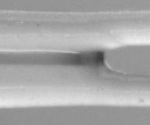
Figure 2. Different imbibition regimes. Pictures show top views of experiments at specified times from the beginning of the experiment. Fibres of radius  $R_0 = 250 \pm 1\,\mathrm {\mu }$m with an initial stretch of $\epsilon = 0.6$ are placed in contact with an oil bath (left side of the picture). Depending on the initial distance $d$ between the fibres, different imbibition regimes are observed. (a) For fibres placed at a large distance, no imbibition is observed. The fibres swell at their base but show no motion of the meniscus. (b) For distances above the Princen criterion (2.2), the meniscus may propagate by swelling the fibres locally. The swelling reduces $d$ and increases $R$ until the imbibition becomes possible. The imbibition also provokes the collapse of the structure once the capillary force overcomes the tension within the fibres. (c) For sufficiently small distances, the imbibition is purely elasto-capillary. Within a few seconds, the meniscus has imbibed far enough to make the fibres collapse. Here, the meniscus reaches the end of the fibres before any significant swelling is noticeable.

Figure 3. Imbibition criterion. (a) Schematic of the cross-section of the fibres before and after swelling at a given position  $z$ along the fibre. As the fibres swell, their radius increases to $\lambda R_s$ (dotted lines), where $\lambda$ is the swelling ratio of the fibres. Here, $d$ also decreases as the fibres swell, which may allow imbibition if criterion (2.2) is reached. (b) Predicted phase diagram showing the type of imbibition depending on $d$ and $R_s$. Using the new values of $d$ and $R$, we obtain a new imbibition criterion. For values of $d$ and $R$ between the two black lines the imbibition is induced by the swelling. The lower line is the upper limit for purely elasto-capillary imbibition. For distances above the second line, the fibres remain too far apart, even after swelling completely.
2.3.2. Imbibition dynamics
Figure 4 presents the measured values of the meniscus position  $z_m$ for fibres of initial radius $R_0 = 250\,\mathrm {\mu }$m. The initial stretch is set to $\epsilon = 0.6$ and the initial distance $d$ between the fibres varies. The oil viscosity is $\eta = 3.2$ mPa s for all experiments. In figure 4(a), we plot the meniscus position as a function of time for different initial values of $d/R_s$. We observe that a higher value of $d/R_s$ leads to a slower overall imbibition. For small initial distances ( $d/R_s < 0.7$), the fibres collapse within a few seconds and the meniscus rapidly progresses towards the end of the fibres. For larger distances ( $d/R_s > 0.7$), the dynamics can be divided into two different parts, illustrated in figure 4(b). After a rapid initial increase of $z_m$ due to the swelling of the fibre portion in contact with the solvent bath at $t=0$, we observe a long swelling-dominated regime. In this regime, the progression of the meniscus is enabled by the local swelling of the fibre, which reduces the interfibre distance. The characteristic times of the swelling are much larger than the typical time scales of a purely elasto-capillary imbibition and we can thus consider the capillary imbibition to be almost instantaneous. The meniscus velocity is thus solely determined by the speed at which the fibre swells. Interestingly, the imbibition occurs at a quasi-constant velocity, which we call $v_{swell}$. We can estimate it experimentally by measuring the slope of $z_m(t)$, as shown in figure 4(b). In the next section, we will attempt to estimate this imbibition velocity based on our understanding of fibre swelling combined with geometrical arguments.

Figure 4. Swelling-induced imbibition: dynamics. (a) Measured meniscus position  $z_m$ vs time for various initial values of $d/R_s$. In these experiments, $R_0 = 250\,\mathrm {\mu }$m and the initial stretch is set to $\epsilon = 0.6$. A larger initial interfibre distance leads to a slower imbibition and a delayed zipping transition. The exact imbibition velocity is very sensitive to the value of $d/R$. (b) Meniscus position vs time for $d/R_s = 1.01$ (also presented in figure 2b.) Insets are the experimental pictures corresponding to the larger dots on the graph. After a rapid initial swelling of the fibre portion in contact with the solvent bath, we observe a long imbibition at a quasi-constant velocity. We call $v_{swell}$ the slope of the curve in the region of swelling-dominated imbibition. When $z_m$ reaches $1$ cm, the meniscus accelerates and we observe the collapse of the structure, which accelerates the meniscus (zipping). We call $l_{zip}$ the distance at which the zipping occurs (details in § 4.).
3. Swelling-induced imbibition velocity
3.1. Simple scaling based on immersed swelling dynamics
Within the region of swelling-induced imbibition, the meniscus can only propagate through the swelling of the fibre portion ahead of  $z_m$. Since the capillary imbibition is a much more rapid phenomenon than swelling (it occurs in seconds, whereas swelling takes minutes), we estimate that the meniscus is always located at the largest possible $z$ for which $d/R < 0.57$. Experimentally, we can confirm this statement by measuring $d$ and $R$ at the meniscus position. As such, as long as elastic effects can be neglected, the concentration profile in the meniscus-centred reference frame is constant, explaining the constant imbibition velocity. To estimate this velocity, we propose a scaling based on the swelling dynamics of an immersed fibre, described in a previous publication (see Van de Velde, Protière & Duprat (Reference Van de Velde, Protière and Duprat2021) and Van de Velde (Reference Van de Velde2022) for more details).
The swelling dynamics of a fibre immersed in a solvent bath can be fitted by the following law:
 \begin{equation} \frac{\lambda(t)-1}{\lambda_{max}-1} = 1-\exp\left({\frac{-t}{T_{swell}}}\right), \end{equation}
where  $T_{swell} = {R_0^2 \eta }/{D^*}$ is a characteristic time scale of the swelling process, and $D^*$ a pseudo-diffusion coefficient that does not depend on the oil viscosity $\eta$, defined so that $D = D^*/\eta$ has the dimension of a diffusion coefficient. A larger fibre or a more viscous oil will lead to a slower overall swelling of the fibre. For simplicity, we will assume that the elastic deformations remain small, i.e. $R_s \simeq R_0$.
The schematic (figure 5a) shows the propagation mechanism we propose. We consider a fibre that is completely dry ahead of the meniscus and swollen behind it. At a time  $t$, the meniscus is located at a position $z_{m}$ for which $d/R = 0.57$ (according to Princen's criterion). To reach $z_m + \mathrm {d}z$, the small fibre portion of length $\mathrm {d}z$ has to swell until $d/R = 0.57$. We call $\mathrm {d}t$ the time necessary to reach this fibre radius. Using the swelling ratio $\lambda (t)$ we can rewrite this condition as
 \begin{equation} \frac{d}{R_0} < 1.57 \lambda({\rm d} t)-1. \end{equation}
By substituting (3.1) we obtain
 \begin{equation} \frac{d}{R_0} < 1.57 \left[ (\lambda_{max}-1)\left( 1-\exp\left({\frac{-{\rm d} t}{T_{swell}}}\right)\right) -1 \right] -1, \end{equation}
which we can simplify to deduce
 \begin{equation} {\rm d} t = T_{swell} \ln \left[\frac{\lambda_{max}-1}{\lambda_{max}-\dfrac{1}{1.57} \left(1+\dfrac{d}{R_0}\right)}\right]. \end{equation}
In all that follows, we will call  $f(d/R)$ the logarithmic function such that ${\rm d} t = T_{swell} f(d/R)$. For $\mathrm {d}z$, $R_0$ is the natural length scale we choose. Indeed, considering our material to be isotropic, as the fluid will diffuse radially towards the centre of the fibre over a distance close to $R_0$, this will lead to a swelling of the order of $R_0$ in the axial direction of the fibres. We thus obtain an estimate for the velocity
 \begin{equation} v_{swell} \simeq \frac{{\rm d} z}{{\rm d} t} = \frac{D^*}{\eta R_0 f(d/R_0)}. \end{equation}
In figure 5(b), we compare the experimental values of  $v_{swell}$ with our scaling. The values are normalized by the natural velocity $D^*/\eta R_0$ emerging from (3.5). The black line presents the value of $1/f(d/R_0)$. We varied the radius of the fibre $R$ and the oil viscosity and find that the data seem to collapse well and are in good agreement with our scaling. In particular, the two asymptotes at $d/R_0 = 0.57$ and $d/R_0 = 1.43$ correspond to the limits obtained in § 2.3. At $d/R = 0.57$, our model assumes an infinite velocity since we do not consider the exact dynamics of the capillary flow. When $d/R_0$ comes close to its upper boundary, the time necessary to swell the fibres becomes extremely long, thus $v_{swell}$ tends to zero.

Figure 5. Estimation of  $v_{swell}$. (a) Schematic explaining the mechanism behind the swelling-induced imbibition. To progress from $z$ to $z+{\rm d}z$, the small fibre portion (dotted black box) has to swell until $d/R = 0.57$ locally. (b) Comparison of the normalized experimental swelling velocities (points) and the values predicted by (3.5) (line). The black line corresponds to $1/f(d/R_0)$. The black diamonds correspond to constant-tension experiments. The imbibition velocity is always lower compared with experiments where the overall stretched length of the fibre was held constant.
The black diamonds in figure 5(b) show the experimental values obtained at constant tension. The experimental set-up used for these experiments is described in figure 1(b). To maintain a constant tension within the fibres during the imbibition, we used long fibres which were clamped at one end and free to slide in the slits of the Plexiglas frame at  $x = L$. The length of the fibres is thus no longer constant. The end of the fibres was attached to a constant mass $m$, thus effectively imposing $T = mg/2$ in each fibre. We find that the velocity is always smaller here than at fixed length/non-constant tension. This shows that tension in the fibre plays a crucial role in the overall imbibition dynamics that is not accounted for in our scaling analysis so far. In the next section, we propose to build a model based on linear poroelasticity, that will justify the validity of our scaling analysis, give more details on the imbibition mechanisms and highlight the role of fibre tension.
3.2. Refined modelling using linear poroelasticity
The scaling analysis made in the previous section gives a good estimation of the imbibition velocity. We will now develop a more detailed model based on linear poroelasticity. This model includes fluid diffusion in the  $z$ direction (which is neglected in the scaling). We will see that it further justifies the choice of length and time scales made previously. Moreover, it will allow us to predict fibre profiles and the evolution of the fibre tension in time and thus compare the two experimental configurations we used. Predicting the tension decrease due to the swelling is also key to understanding the elastocapillary collapse that we observe in our experiments.
3.2.1. Model equations
We model our fibres in the framework of linear poroelasticity based on Biot's theory developed for fluid imbibition in soils (Biot Reference Biot1941; Hui & Muralidharan Reference Hui and Muralidharan2005; Dervaux & Ben Amar Reference Dervaux and Ben Amar2012). This model was adapted to model the absorption of fluid drops on fibres in a previous study (Van de Velde et al. Reference Van de Velde, Dervaux, Protière and Duprat2022).
The fibre is considered as a poro-elastic material, which can be described by three different quantities: the local solvent concentration  $c$, the chemical potential $\mu$ and a displacement field $\boldsymbol {u}$. The initial values in the absence of any mechanical load are homogeneous in the fibre, $c = c_0$ and $\mu = \mu _0$. The chemical potential in the fluid outside the fibre is set at $\mu = \mu _b$. When the fibre touches the solvent, if $\mu < \mu _b$, solvent will flow into the poroelastic network. By symmetry, we can consider only one of the two fibres. The solvent concentration within the fibres can be linked to the deformations of the material described by the displacement field $\boldsymbol {u}$. The initial stretch applied to the fibre is $\epsilon = {L}/{L_0}-1$. For simplicity, we do not consider any deflection of the fibres due to the capillary force in the meniscus. The objective of the model is to give a prediction for the spatio-temporal evolution of the solvent concentration $c(z,t)$. The derivation of all the equations is detailed in Appendix A. For simplicity, we will only focus on the essential equations in this section. After simplifications due to the mainly one-dimensional geometry of the fibres, we obtain the following equation describing the solvent concentration along the fibre:
 \begin{equation} \frac{\partial c}{\partial t} = D\frac{\partial ^2 c}{\partial z^2} + \frac{2D}{R_0 h}(c_{max}(t) - c) \boldsymbol{1}_d(z,t), \end{equation}
which contains a diffusing term, with a diffusion coefficient  $D = D^*/\eta$, and a source term, where the fibres are in contact with the liquid with a length scale $h$ characterizing the flow of fluid across the fibre interface that is of the order of the fibre radius (Van de Velde et al. Reference Van de Velde, Dervaux, Protière and Duprat2022). Here, $\boldsymbol {1}_d(z,t) = 1$ if $z < z_m$ and 0 elsewhere. The maximal possible concentration in the fibre is given by
 \begin{equation} c_{max}(t) = c_0 + \frac{3(1-2\nu)}{2G\varOmega^2(1+\nu)}\left(\mu_b - \mu_0 + \frac{\varOmega \sigma_{zz}(t)}{3}\right), \end{equation}
where  $\varOmega$ is the molar volume of the solvent, $\nu$ is the poro-elastic Poisson ratio and $\mu _b$ is the chemical potential in the drop (outside the polymer). Equation (3.6) can be understood as a one-dimensional diffusion equation with a source term depending on the position of the meniscus and the local concentration of solvent within the fibre. For simplicity, we consider the source to be surrounding the fibre rather than located on one side of the fibres only, although this effect could easily be incorporated by adding a prefactor proportional to the fraction of the fibre perimeter in contact with the solvent to the second term on the right-hand side of (3.6). Moreover, we consider the swelling to be homogeneous across the fibre section, which is an approximation that we discuss later.
The tension in the fibre is found by integrating the concentration over the fixed length of the fibre, i.e.
 \begin{equation} \sigma_{zz}(t) = 3G\epsilon - \frac{G\varOmega}{L} \int_{0}^{L}(c-c_0)\,\mathrm{d}z. \end{equation}
We can also deduce the radial displacement along the fibre by calculating
 \begin{equation} u_r(r,z,t) = r \frac{2(c- c_0)G\varOmega - \boldsymbol{\sigma}_{zz}(t)}{6G}, \end{equation}
with  $r$ the coordinate in the radial direction of the fibres and $G = {E}/{3}$ the shear modulus of the polymer. In fact, by combining (3.6), (3.7) and (3.8), one obtains an integro-differential equation. Complex effects arise from the fact that the equilibrium concentration in the fibre depends on the current tension, which in turn depends on the total amount of fluid that has diffused into the fibre.
We opt for no-flux boundary conditions at  $z = 0$ and $z = L$ in the constant length configuration. At constant tension, we have a no-flux boundary condition at $z = 0$ and $c = 0$ at $z = \infty$. To solve for the meniscus position, we also need to evaluate the position of the meniscus. By considering the capillary imbibition to be instantaneous compared with the poroelastic diffusion within the fibres, we find $z_m(t)$ as the largest value of $z$ verifying $d(z,t)/R(z,t) <0.57$. This is done numerically at each time step.
We will now solve this set of equations first analytically at constant tension and then using finite differences.
3.2.2. Solution at constant tension
In all that follows, we consider  $c_0 = 0$ for simplicity, as this does not change the reasoning made in this section. We simplify the equations by considering a constant tension such that $\sigma _{zz} = \sigma _0 = 3G\epsilon$ at all times. Considering (3.8), this holds as long as the integral term is small compared with $3G\epsilon$. If $z_m/L = 0.2$, assuming the fibre is fully swollen behind the meniscus, the associated change in stress is $\Delta \epsilon = {L}/{L_0}-{L}/{(1+0.2(\lambda _{max}-1))L_0} = 0.1 \epsilon$. Taking this as a limit, we assume that, as long as $z_m/L < 0.2$, this simplification is reasonable, thus allowing us to use it to estimate $v_{swell}$. The maximal concentration within the fibre is thus constant. Considering the capillary imbibition to be instantaneous relative to the swelling process, we can still assume that $d/R = 0.57$ at the meniscus position. As $d$ and $R$ can be evaluated from the radial displacement, this is written as
 \begin{equation} \frac{d-u_R}{R_0+u_R} = 0.57. \end{equation}
Knowing  $u_R$ from (3.9), we can rewrite (3.10) as
 \begin{equation} d-R_0\left(\frac{2c_m G\varOmega - 3G\epsilon}{6G}\right) = 0.57R_0 \left(1+\frac{2c_m G\varOmega - 3G\epsilon}{6G}\right), \end{equation}
and, after isolating  $c_m$, we obtain
 \begin{equation} \varOmega c_m = 3 \frac{d-0.57 R_0}{1.57R_0} + 3 \frac{\epsilon}{2}. \end{equation}
The maximal concentration within the fibre can also be deduced as a function of the maximal swelling ratio  $\lambda _{max}$. At a constant tension, $c_{max}$ is a constant (as is $\lambda _{max}$). Knowing that $u_{R, max} = (\lambda _{max}-1)R_0$, and using (3.9) with $c = c_{max}$ we obtain
 \begin{equation} \varOmega c_{max} = 3(\lambda_{max}-1) + \tfrac{3}{2} \epsilon. \end{equation}
In the steady state (far from  $z=0$ and $z=L$), the meniscus propagates at a constant velocity $v_{swell}$, thus $z_m = v_{swell}t$ and we can rewrite (3.6) as
 \begin{equation} \frac{\partial c}{\partial t} = D\frac{\partial ^2 c}{\partial z^2} + \frac{2D}{R_0h}(c_{max}(t) - c) \theta(v_{swell}t-z), \end{equation}
where  $\theta$ is the Heaviside function. Note that the steady-state solution only exists at a constant tension.
Placing ourselves at the meniscus position such that  $z' = v_{swell}t-z$, we can rewrite our equation as
 \begin{equation} \frac{\partial^2 c}{\partial z'^2} + \frac{v_{swell}}{D} \frac{\partial c}{\partial z'} + \frac{2}{R_0 h}(c_{max} - c)\theta(z') = 0. \end{equation}
We consider a fibre of infinite length (i.e. that the meniscus is very far from the clamps). The boundary conditions on the concentration are then as follows:
 \begin{equation} c(z') = \left\{\begin{array}{@{}ll} c_m, & z' = 0 \\ c_{max}, & z' =-\infty \\ 0, & z' =+\infty. \end{array}\right. \end{equation}
We find the solutions ahead and behind the meniscus separately and get the following solutions:
 \begin{equation} c(z') = \left\{\begin{array}{@{}ll} c_m \exp\left({-\dfrac{v_{swell}}{2D}z}\right), & z' > 0 \\ c_{max} + (c_m - c_{max})\exp\left({\left(-\dfrac{v_{swell}}{2D} + \dfrac{1}{2}\sqrt{\left(\dfrac{v_{swell}}{D}\right)^2 + \dfrac{8}{R_0 h}}\right)z'}\right), & z' < 0. \end{array}\right. \end{equation}
The continuity of flux at  $z' = 0$ then gives us
 \begin{equation} \frac{\partial c}{\partial z'}(z' = 0^-) = \frac{\partial c}{\partial z'}(z' = 0^+), \end{equation}
and after rearranging
 \begin{equation} c_m = c_{max}\left(1-\frac{1}{\sqrt{1+\dfrac{8D^{2}}{v_{swell}^2R_0h}}}\right). \end{equation}
Replacing  $c_{max}$ with (3.13) and comparing the expressions obtained for $c_m$ in (3.12) and (3.19) we get, after a few lines of algebra, the following expression for $v_{swell}$:
 \begin{equation} \frac{v_{swell}\sqrt{R_0h}}{D} = 2\sqrt{2} \left(\left(\frac{\lambda-1 + \epsilon/2}{\lambda-1 - \dfrac{d-0.57R_0}{1.57R_0}}\right)^2-1\right)^{-1/2}. \end{equation}
We can thus define  $V^* = {D}/{\sqrt {R_0h}}$ as the natural velocity of our system. Note that, if $h=R_0$ (which is the case in previous studies Van de Velde et al. Reference Van de Velde, Dervaux, Protière and Duprat2022), one recovers the natural velocity found by our scaling developed in the previous section. An increase in stretch will lead to a decrease of $v_{swell}$ since $R_s$ will decrease slightly due to the elastic Poisson effect, the distance between the fibres will thus slightly increase. An increase in $\epsilon$ can thus be related to an increase in $d/R_s$. The maximal swelling ratio has little effect on $v_{swell}$, but rather on the limit values of $d/R_s$. Figure 6 shows the normalized velocity calculated with (3.20) (red solid line) compared with our previous scaling (black solid line). The analytical solution is similar to our scaling, thus confirming the length and time scales we chose before. Differences between the poro-elastic model and the scaling become visible at large values of $d/R_0$, as diffusion in the axial direction plays a larger role. The red crosses present the values of $v_{swell}$ obtained by solving our model numerically at a constant zero tension. The results overlap with our analytical solution, which means we can trust our numerical scheme to find the solution at a time-dependent tension using this method. The deviations between the analytical solution and the simulations at large values of $d/R_0$ can be attributed to the finite size of the fibres in the simulation, which is not the case for the analytical solution (3.16). Our analytical solutions (and the scaling) both agree well with our data, even though they are evaluated at a constant, zero tension, whereas the experimental data are obtained at non-zero time-dependent tension. The scatter of the data at small values of $d/R_0$ is mainly due to the fact that the cross-over between the regime of quasi-constant velocity and the acceleration due to elasto capillary effects happens sooner, thus decreasing the period over which $v_{swell}$ can be measured. This might also lead to a slightly higher measured velocity compared with the constant-tension models. The red squares show the results of the simulation for a constant tension corresponding to the same stretch of $\epsilon = 0.3$ as the experiments described in the previous section (black diamonds). We have a good agreement between our experiments and the numerical simulations. This means that, in reality, our scaling slightly overestimates the value of $v_{swell}$. The good agreement between the experimental data obtained at a constant length and the scaling is fortunate and probably due to the elasto-capillary deflection of the fibres or the fact that the swelling is not uniform across the fibre cross-section. Our poro-elastic model can predict the imbibition velocity accurately in the absence of elasto-capillary deflection. To estimate this deflection, it is key to understand the evolution of the fibre tension throughout the experiment. In section (3.2.3), we solve our equations with a variable tension, which allows us to predict the evolution of the fibre tension over time. This will also allow us to understand the acceleration of the meniscus observed before the zipping transition.

Figure 6. Poroelastic estimation of  $v_{swell}$. Normalized experimental values of $v_{swell}$ (points) compared with our scaling (black), the analytical solution of the poroelastic model (3.20) (red line) and the values of $v_{swell}$ found by solving the model numerically with a constant zero tension (red crosses) and constant non-zero tension ( $\epsilon _0 = 0.3$, red squares) (§ 3.2.3). Black diamonds correspond to values found experimentally at a constant non-zero tension ( $\epsilon = 0.3$).
3.2.3. Solving the equations with a time-dependent tension
In our experiments, as the fibres swell and expand both radially and axially, the tension in the fibre decreases over the course of the imbibition since its total stretched length is maintained constant. To quantify the effects of this decrease in tension we solve (3.6) with a time-dependent tension using a finite difference scheme of order 1. Note that, in this case, the fibres still stay straight and are not deflected by capillary forces. Figure 7(a) shows fibre profiles at regular intervals during the imbibition. Lighter curves correspond to later times. The meniscus position at each step is represented by the vertical grey lines. By looking at the position of the fibre/air interface at large values of  $z$ we can see that the fibre radius increases far away from the meniscus. This is due to the relaxation of the axial constraint (3.8) induced by the absorption of liquid. This relaxation will effectively increase $R$ and decrease $d$ over time, both in the swollen and in the dry regions of the fibre. This time evolution explains the acceleration of the meniscus observed numerically and experimentally. The predicted meniscus position when including the effects of a time-dependent tension in the model is plotted against time in figure 8(a) for different values of $d/R_0$ (solid lines). The dashed lines correspond to simulations at a constant tension, equivalent to the initial tension in the time-dependent tension calculation. Note that, at constant tension, apart from the initialization at very small times, for which $z_m$ is constant (figure 8b), the meniscus velocity is strictly constant. The initial plateau, both for time dependent and constant tension, corresponds to the swelling of the small fibre section initially touching the bath, which first needs to reach Princen's criterion before allowing a progression of the meniscus. As in the experiment, a smaller interfibre distance leads to faster imbibition. For the smallest value of $d/R_0$ (darkest curve), the simulation is stopped before the meniscus reaches the end of the model pore. We can stop the simulation once $d/R = 0.57$ even in unswollen regions of the fibre since the imbibition then becomes purely capillary. We also recover the fact that the imbibition happens at a quasi-constant velocity at a small value of $z_m$. We estimate the values of $v_{swell}$ by considering the slope of $z_m = f(t)$ once the imbibition starts. In fact, it is identical to values obtained with a constant tension, provided the initial values of $\epsilon _0$ are the same (cf. figure 8a). The elastocapillary deflection being highly dependent on the fibre tension, we calculate the predicted axial stress $\sigma _{zz}$ within the fibres using (3.8). Figure 8(c) shows that the axial stress reduces a lot during the absorption. This causes an overall increase in fibre radius, as detailed before. When plotted against the meniscus position (figure 8c), all the values of stress collapse, meaning that the stress depends only on the meniscus position $z_m$. Since the overall stress depends solely on the total amount of fluid absorbed by the fibre, this can only be true if the size of the region of variable concentration (around the meniscus) is very small compared with the overall fibre size. This further justifies the approximation made for our scaling, where we suppose the transition between swollen and dry fibre to be located exactly at the meniscus position. In reality, this is not entirely true. From the profiles of figure 7 we see that the region in which $0 < c < c_{max}$ has a non-zero extension (figure 7c). A slight deviation can also be observed in figure 8(d) for small values of $d/R$ (purple curve). If $d/R$ is small, the progression of the meniscus is fast and the fibre has less time to swell behind $z_m$. In other words, the portion of the fibre with a spatially variable concentration is larger).

Figure 7. Simulated fibre profiles. (a) Fibre profiles obtained with our full poroelastic model. Coloured lines represent the inner edge of each fibre at different times (regular intervals, see hatched region of the schematic above). Grey lines denote the meniscus position. We can reproduce the swelling-induced imbibition. The fibre radius close to  $z = 3$ cm increases as the swelling causes the tension to decrease. This leads to a progressive acceleration of the meniscus. (b) Overlap of simulated profiles and experimental pictures for different meniscus positions. Simulation and experiment are in good agreement. Differences exist at the outer edges of the fibres since the model does not take the asymmetry of the problem into account. (c) Zoom on the meniscus (red square in (b)) showing the complex three-dimensional shape of the contact line.

Figure 8. Simulated values of  $z_m$ and tension. (a) Simulated meniscus position for different values of $d/R_0$ obtained with an initial stretch $\epsilon _0 = 0.3$ with a time-dependent tension. For $d/R_s = 0.67$ the simulation stops once $d/R = 0.57$ in the non-swollen region of the fibres. Dashed lines correspond to the constant-tension case. Panel (b) shows a close-up of the initial minutes of the simulation. A small portion of the fibres (2 mm) is in contact with the fluid bath and swells but $z_m$ remains constant. As soon as Princen's criterion is met, the imbibition starts. The initial slopes (thus the values of $v_{swell}$) match for the constant and time-dependent tension experiments as the initial values of stretch are the same. (c) Corresponding values of the normalized axial stress as a function of time. The further the fibres are apart, the slower the imbibition and the slower the tension decrease. (d) Normalized axial stress as a function of the meniscus position. All the curves seem to collapse onto the same curve. Slight differences come from the difference in swelling at the meniscus position, which is necessary to start the imbibition process. Once the fibre relaxes enough, $d/R$ in the dry region comes closer to 0.57, speeding up the meniscus, leading to a deviation from the common curve.
A time-dependent tension thus tends to increase the imbibition velocity compared with the constant tension case, an effect observed both in experiments and numerics. We have seen in this section that our model including the tension tends to under-estimate the value of  $v_{swell}$ in all cases. It thus seems that, in our experiments, an additional effect leads to an increase of the velocity. A good candidate for this is the elastocapillary deflection due to the presence of fluid between the fibres. In the next section, we aim to estimate this deflection and the position of the meniscus at which the zipping transition occurs using a simple mechanical model.
4. Elastocapillary collapse
We mentioned several times that the fibres later on undergo an elastic collapse. We now wish to describe this, as well as the rapid acceleration of the meniscus that occurs in the final stages of most of our experiments. It is triggered once the capillary force exerted by the meniscus overcomes the restoring tension force in the fibres. The elastocapillary collapse of fibrous structures has been described on arrays of fibres exposed to fluid baths (Bico et al. Reference Bico, Roman, Moulin and Boudaoud2004; Bico, Reyssat & Roman Reference Bico, Reyssat and Roman2018) or drops (Duprat & Protiere Reference Duprat and Protiere2015) as well as during the capillary imbibition between flexible plates (Aristoff et al. Reference Aristoff, Duprat and Stone2011; Duprat et al. Reference Duprat, Aristoff and Stone2011). In all cases, the capillary force exerted by the fluid overcomes either the bending stiffness of the solid or a tension force that tends to keep the solids separated. In the case of swelling PVS plates, the deformations induced by swelling can induce motion of a fluid drop, which advances by swelling the elastomer and keeping the two plates together via capillary forces (Holmes et al. Reference Holmes, Brun, Pandey and Protière2016). The time scales of the elastic collapse are of the order of a few seconds, which is much smaller than the typical time scales of swelling. This collapse is thus a pure elasto-capillary effect. In this section, we wish to understand the role swelling can play on the meniscus position at which the collapse can occur.
Over the course of the imbibition, the tension within the fibres will decrease due to the swelling, while the capillary force increases as the overall length of the contact line increases. We call  $l_{zip}$ the position of the meniscus at which the zipping occurs. We define it as the point of maximum acceleration of the meniscus (figure 4(b); details are given in Appendix B).
To predict the position of the meniscus at which the zipping occurs, we calculate the maximum deflection  $\delta$ of the fibres (i.e. the deflection at the meniscus position). Our zipping criterion is the following:
 \begin{equation} \frac{d-\delta}{R} < 0.57. \end{equation}
In other words, the elastocapillary deflection alone is sufficient to allow the imbibition without needing to further swell the fibres. Since the elastocapillary imbibition is much quicker than the swelling-induced imbibition, the meniscus speeds up significantly. As it progresses, the capillary force also continues to increase until, eventually, the fibres come into contact. To predict the deflection analytically, we consider a fibre composed of two rigid rods connected at the meniscus position (figure 9a). We estimate the capillary force to be constant over the entire wetted length and neglect the saddle shape of the meniscus (i.e. assuming  $z_m \gg d$) giving a force per unit length
 \begin{equation} \mathrm{d}F_c = 2 \gamma. \end{equation}
The factor 2 comes from the fact that there is one contact line on each side of the fibre. When summing all forces, it becomes equivalent to a point force  $F_c = 2 \gamma z$ exerted at the centre of the left rod. A balance of moments gives us the following relationship between capillary and axial tension forces:
 \begin{equation} T\sqrt{z^2+\delta^2} \sin (\phi_1 + \phi_2) = \frac{\sqrt{z^2+\delta^2}}{2}2\gamma z \cos \phi_1, \end{equation}
where  $T$ is the tension force within the fibre, and $\phi _{1,2}$ the angles between the fibre and the horizontal position (as shown in figure 9). After expanding the $\sin$ and rearranging the terms
 \begin{equation} \tan \phi_1 \cos \phi 2 + \sin \phi_2 = \frac{\gamma z}{T}. \end{equation}
This gives, at first order in  $\phi _{1,2}$ considering small angles (and thus small deflections ${\delta }/{L} \ll 1$),
 \begin{equation} \frac{\delta}{z} + \frac{\delta}{L-z} = \frac{\gamma z}{T}, \end{equation}
and finally the deflection depending on the meniscus position
 \begin{equation} \delta(z) = \frac{\gamma z^2(L-z)}{LT}. \end{equation}
An estimate of the fibre tension can be found by considering a fibre fully swollen for  $z< z_m$ and dry for $z> z_m$. We can then estimate the change in unstretched length $L_0$ using the maximal swelling ratio $\lambda _{max}$ giving for the tension
 \begin{equation} T = E{\rm \pi} R_0^2 \epsilon = E{\rm \pi} R_0^2\left(\frac{L}{L_0+ (\lambda_{max}-1)z_m}-1\right). \end{equation}
Equation (4.7) is a simplified version of (3.8) but gives very similar results as shown in figure 11; see Appendix C. We thus use it here for simplicity to find an estimation for  $l_{zip}$. We can combine (4.1) and (4.7) to obtain the following equation for $l_{zip}$:
 \begin{equation} \frac{\gamma l_{zip}^2(L-l_{zip})(L_0+\lambda_{max}-1)l_{zip})}{LE{\rm \pi} R_0^2 (L-L_0-(\lambda_{max}-1)l_{zip})} = d-0.57R_0. \end{equation}
The solutions for (4.8) are shown in figure 9. Here,  $l_{zip}$ is plotted against $d/R_0$ for different values of the initial stretch. All curves and data points are obtained for fibres having an initial radius of $250\,\mathrm {\mu }$m. The colours of the experimental points and modelled values (lines) have matching colours corresponding to different values of $\epsilon$; $l_{zip}$ is undefined for $d/R_0 < 0.57$ since the imbibition will then always be elastocapillary and $l_{zip}$ increases with the stretch, which is intuitive as it then becomes more difficult to deflect the fibres. At high stretches, the fibres will also have to be deflected more, explaining why $l_{zip}$ also increases with $d/R_0$. The data and curves are in good qualitative agreement. Several limitations to our model might explain the discrepancies between model and experiment. First, the definition of $l_{zip}$ is slightly ambiguous as elastocapillary imbibition will not cause the fibres to collapse at $z=0$. The estimation of the capillary force is also simplified. The exact position of the triple line on the fibres is hard to determine and is highly dependent on the local distance between the fibres. The exact radius of the fibres is also estimated roughly here, as we consider a fibre fully swollen behind the meniscus and dry in front of it. Finally, the exact shape of the meniscus is three-dimensional and thus the force exerted on the fibres at $z = z_m$ is prone to errors here. For small values of $d/R_0$, the imbibition is relatively fast and the fibres may not have the time to swell completely behind the meniscus. For small values of stretch (dark purple points in figure 9) in particular, the assumption that the fibre is fully swollen behind the meniscus is certainly wrong as the deflection of the fibres leads to relatively fast imbibition, even at small times. This could explain why the experimental value of $l_{zip}$ is actually decreasing with $d/R_s$. For larger values of $d/R_s$, the fibres have the time to swell at an equivalent meniscus position, the tension is actually lower than for small values of $d/R_s$. To correct this, the model would need to include the transient swelling dynamics and couple it to the dynamics of the capillary flow between two fibres, which is beyond the scope of this study.

Figure 9. (a) Notations used to calculate the deflection due to the capillary force. The fibre is assumed to be composed of two rigid rods connected at  $z = z_m$. Here, $\phi _{1,2}$ are the deflection angles at $z=0$ and $z=L$. To predict the deflection we equal the moments exerted in 0 by the capillary force (green arrow) and the tension $T$ within the fibre (red arrow), which gives (4.3). (b) Estimated value of the length at which the imbibition becomes elasto-capillary ( $l_{zip}$) for different values of $\epsilon$ and $d/R_s$. The points correspond to experimental values. Here, $l_{zip}$ is fixed at the point of highest acceleration of the meniscus.
5. Discussion and conclusion
In this study, we have described the elasto-capillary imbibition in a model pore composed of two swellable fibres. We have shown that swelling enables imbibition even for fibres that are a priori too far apart, i.e. above Princen's criterion. The fibres are brought closer together by swelling, leading to swelling-induced imbibition. By extending the imbibition criterion established by Princen, we have found the upper limit for the interfibre distance allowing this new kind of imbibition. Contrary to the purely capillary case, this imbibition occurs at a constant velocity, which can be estimated via a scaling analysis. By deriving and solving a more complex model based on linear poro-elasticity, we were able to confirm the choices of length and time scales chosen for the scaling. The model is in good agreement with the experimental data performed at a constant tension, for which the elasto-capillary deflection is less important than for fibres kept at a constant length. The deflection of the fibre is a result of the competition between the tension within the fibres and the capillary forces exerted by the fluid. Its effect is to slightly accelerate the meniscus’ motion as the fibres are brought closer together. Eventually, it even leads to the elastic collapse of the model pore (zipping of the fibres). To describe the deflection and predict when zipping can occur, it is important to understand how the fibres’ tension decrease over the course of the experiment. This evolution is well described with the poro-elastic model. In a final section, we proposed an estimation of the deflection with a simplified model of our fibres. In order to predict the precise imbibition velocities, a model coupling the precise dynamics of the capillary flow with the swelling and the elasto-capillary deflection would be needed. In real-life fibrous systems, such as paper sheets or fabrics, the fibres are often much more constrained and therefore less deflection by the fluid is possible. In addition, several pores can be adjacent and capillary forces exerted on a fibre might thus come from both sides, limiting the deflection.
As mentioned, another limitation of our models comes from the wetting of the fluid around and between the fibres. In our poro-elastic model, we consider a fluid source surrounding the fibres, which is incorrect as the fluid is in reality located between the fibres (Princen Reference Princen1969). This non-symmetric location of the fluid leads to an asymmetric swelling, (figure 7). Indeed, the inner part of the model pore swells at a slightly faster pace than its outer part. Describing the exact position of the fluid around and within a three-dimensional fibre is a challenging endeavour beyond the scope of our present study. As the characteristic length scale of the meniscus is small compared with the length of our fibre, we believe it could change the estimations of  $v_{swell}$ but not affect the described mechanisms for swelling-induced imbibition and elastic collapse of our structure. Again, in the case of adjacent pores, this asymmetry might be lost as fluid could diffuse within the fibre from both sides.
In this work, the time scales for the capillary imbibition and the swelling are different, which allows for decorrelating of their effects in the models. A natural extension of this work would be to consider different materials, for which the capillary and swelling time scales become comparable.
Declaration of interests
The authors report no conflict of interest.
Appendix A. Derivation of the poro-elastic equations
We model our experiment in the framework of linear poroelasticity. The fibre is considered as a poro-elastic material, which can be described by three different quantities: the local solvent concentration  $c$, the chemical potential $\mu$ and a displacement field $\boldsymbol {u}$. The initial values in the absence of any mechanical load are $c = c_0$ and $\mu = \mu _0$. The chemical potential in the fluid outside the fibre is set at $\mu = \mu _b$. When the fibre touches the solvent, if $\mu < \mu _b$, solvent will flow into the poroelastic network. We will start by deriving the equations describing the solvent motion within the network as well as the associated deformations of the fibre. We will then add a source term to the equations, linked to the presence of solvent at the outer boundary of the fibres.
Within the fibre, the conservation of the number of solvent molecules writes
 \begin{equation} \frac{\partial c}{\partial t} + \boldsymbol{\nabla} \boldsymbol{\cdot} \boldsymbol{J} = 0, \end{equation}
where  $\boldsymbol {J}$ is the flux of the solvent in the gel, due to gradients in chemical potential. The flux $\boldsymbol {J}$ of small molecules can be described by Darcy's law
 \begin{equation} \boldsymbol{J} =- \left(\frac{k}{\eta \varOmega^2}\right) \boldsymbol{\nabla}\mu, \end{equation}
where  $k$ is the permeability, $\eta$ is the viscosity of the solvent and $\varOmega$ is the molar volume of the solvent.
The strain tensor  $\boldsymbol \epsilon$ is defined as
 \begin{equation} \boldsymbol{\epsilon} = \tfrac{1}{2} \left( \boldsymbol{\nabla}\boldsymbol{u} + (\boldsymbol{\nabla} \boldsymbol{u})^t \right). \end{equation}
In the framework of linear poroelasticity, the stress tensor  $\boldsymbol {\sigma }$ is given by
 \begin{equation} \boldsymbol{\sigma} = 2G \left(\boldsymbol{\epsilon} + \frac{\nu}{1-2\nu} {\rm Tr}(\boldsymbol{\epsilon}) \boldsymbol{\mathsf{I}} \right) - \frac{\mu-\mu_0}{\varOmega}\boldsymbol{\mathsf{I}}, \end{equation}
where  $G$ is the shear modulus, $\nu$ is the poroelastic Poisson ratio and $\boldsymbol{\mathsf{I}}$ is the identity tensor. The poroelastic Poisson ratio describes how much fluid can be absorbed by a given material. If $\nu = 1/2$ there is no swelling. A direct measurement of this quantity is complex. Most studies assume a value of $\nu = 1/3$ for usual elastomers. We assume that solvent and polymer molecules are incompressible. Thus any variation of the polymer volume can be linked to the solvent concentration. The incompressibility condition writes
 \begin{equation} Tr(\boldsymbol{\epsilon}) = (c-c_0)\varOmega. \end{equation}
The mechanical equilibrium in the bulk of the poroelastic material is described by the Navier equations
 \begin{equation} \boldsymbol{\nabla} \boldsymbol{\cdot} \boldsymbol{\sigma} = \boldsymbol{0}. \end{equation}
Combining the equations above we get
 \begin{equation} \frac{\partial c}{\partial t} = D^* \Delta c, \end{equation}
where
 \begin{equation} D^* = \frac{2(1-\nu)Gk}{(1-2\nu)\eta}, \end{equation}
is an effective diffusion coefficient and  $\varDelta$ is the Laplace operator. The material parameters $G$,
$G$,  $k$ and thus $D^*$ are effective parameters that depend on the initial state of the gel. Finally, combining (A3), (A4), (A5) and (A6), we get
 \begin{equation} G \varOmega \left(\Delta \boldsymbol{u} + \frac{\varOmega}{1-2\nu} \boldsymbol{c} \right) = \boldsymbol{\nabla} \mu. \end{equation}
To simplify this equation, we perform a dimensionality reduction by assuming our fibres are thin ( $R \ll L$) and consider time scales larger than $R^2/D^*$. This is a time comparable to the time scale $\tau _{swell}$ introduced in our scaling analysis, representing the time it takes for solvent molecules to reach the fibre core. We will now consider that the concentration and thus the chemical potential are approximately constant throughout the radius of the fibre such that the problem will become effectively two-dimensional ( $z$ and time $t$). This translates into the following assumptions:
 $$\begin{gather} c(r,z,t) = \bar{c}(z,t), \end{gather}$$
 $$\begin{gather}\mu(r,z,t) = \overline{\mu(z,t)}. \end{gather}$$
For consistency with our approximation, we assume that physical quantities vary over a typical length scale  $L$ in the axial direction $z$ while they vary over a typical length scale $R$ in the radial direction $r$. At leading order in $R/L$, since $R \ll L$, the $r$-component of the mechanical equilibrium equations (A9) thus implies
 \begin{equation} \frac{1}{r}\frac{\partial}{\partial r} \left(r \frac{\partial u_r}{\partial r} - \frac{u_r}{r^2}\right) = 0. \end{equation}
The only solution of (A12) that vanishes at  $r = 0$ is of the form
 \begin{equation} u_r(r,z,t) = r \overline{u_r}(z,t). \end{equation}
The molecular incompressibility (A5) further implies that the axial displacement is independent of  $r$ at leading order
 \begin{equation} u_z(r,z,t) = \overline{u_z} (z,t). \end{equation}
From the results above, we deduce that the radial stress  $\sigma _{rr}$ and shear stress $\sigma _{rz}$ are solely functions of $z$ and $t$, at leading order in $R=L$. The stress-free boundary condition at the surface ( $\boldsymbol {\sigma } \boldsymbol {\cdot } \boldsymbol {n} = \boldsymbol {0}$ at $r = R$) thus gives us
 \begin{equation} \sigma_{rr} = \sigma_{rz} = 0. \end{equation}
Therefore, we can obtain from (A9)
 $$\begin{gather} u_r(r,z,t) = r \frac{2(\bar{c} - c_0)G\varOmega - \boldsymbol{\sigma}_{zz}(t)}{6G}, \end{gather}$$
 $$\begin{gather}\frac{\partial \bar{u}_z}{\partial z}=\frac{(\bar{c} - c_0)G\varOmega - \boldsymbol{\sigma}_{zz}(t)}{6G}, \end{gather}$$
 $$\begin{gather}\bar{\mu}(z,t) = \mu_0 + \frac{2G\varOmega^2(1+\nu)}{3(1-2\nu)}(\bar{c}-c_0) - \frac{\varOmega \boldsymbol{\sigma}_{zz}(t)}{3}. \end{gather}$$
If we find an expression for the stress  $\sigma$ and the concentration $c$, we will be able to find the deformation field $\boldsymbol {u}$. For now, we have not introduced the solvent source coming from the capillary flow. Here, $c$ and $\sigma _{zz}(t)$ can be calculated from the boundary conditions and transport equation, which reads in cylindrical coordinates,
 \begin{equation} \frac{\partial \bar{c}}{\partial t} + \frac{1}{r} \frac{\partial(rU_r)}{\partial r} + \frac{\partial J_z}{\partial z} =0, \end{equation}
where  $J_z$ is the flux in the lengthwise direction. Integrating (A19) over the section of the fibre gives
 \begin{equation} \frac{\partial \bar{c}}{\partial t} + \frac{2J_r^s}{R} + \frac{\partial J_z}{\partial z} =0, \end{equation}
where  $J_r^s$ is the surface flux of solvent coming into the fibre. It is present for all values such that $z< z_m$. We assume that the fluid surrounds the fibre completely (behind the meniscus), even though in reality it sits only on the inner part of the fibres. This approximation allows us to make the dimensionality reduction described above. Without this, a complete three-dimensional model of the fibre would be necessary. We therefore cannot here reproduce the exact asymmetric deformations observed in the experiments. Nonetheless, this approach gives a good estimation of the overall deformations and dynamics.
For  $z< z_m$, $J_r^s$ is simply proportional to the difference between the chemical potential in the fluid $\mu _b$ and the chemical potential in the fibre $\mu$. If $z>z_m$, we assume that the fibre is impermeable and this flux is zero. Utilizing (A18) we can write this flux as
 \begin{align} J_r^s &=-\frac{k \boldsymbol{1}_d(z,t)}{\eta \varOmega^2h}(\mu_b - \bar{\mu}) \nonumber\\ &=-\frac{k \boldsymbol{1}_d(z,t)}{\eta \varOmega^2h}\left(\mu_b - \mu_0 + \frac{\varOmega \sigma_{zz}(t)}{3} - \frac{2G\varOmega^2(1+\nu)}{3(1-2\nu)}(\bar{c}-c_0)\right), \end{align}
where  $h$ is a length (presumably microscopic) that characterizes the interface such that the quantity $k/2h$ is a surface permeability. The function $\boldsymbol {1}_d(z, t)$ is indicative of the source: it is a function which value is 1 if there is a fluid in contact with the fibre at position $z$ and time $t$ and which value is zero otherwise. We finally obtain the following equation, which is essentially a diffusion equation with a source term wherever some solvent is touching the fibres:
 \begin{equation} \frac{\partial \bar{c}}{\partial t} = D\frac{\partial ^2 \bar{c}}{\partial z^2} + \frac{2D}{Rh}(c_{max}(t) - \bar{c}) \boldsymbol{1}_d(z,t), \end{equation}
where the time-dependent equilibrium concentration  $c_{max}(t)$ is
 \begin{equation} c_{max}(t) = c_0 + \frac{3(1-2\nu)}{2G\varOmega^2(1+\nu)}\left(\mu_b - \mu_0 + \frac{\varOmega \sigma_{zz}(t)}{3}\right). \end{equation}
The effective diffusion coefficient  $D$ appearing in (A22) is $D = {2kG(1+\nu )}/{3\eta (1-2\nu )}$. Interestingly, the maximal concentration within the fibres and thus the value of the maximal swelling coefficient $\lambda _{max}$ depends on the current tension within the fibres. The change in $c_{max}$ over the course of the experiment has been described in a previous study focusing on the absorption of drops (Van de Velde et al. Reference Van de Velde, Dervaux, Protière and Duprat2022). The effect of this change is less important for the capillary imbibition as elasto-capillary effects and the error due to the symmetry assumption are significant.
The model also gives us an equation for the tension in the fibre. This equation is provided by the boundary condition at the end of the fibre. For the experiments at constant length, the initial displacement of the fibre is known from the pre-stretch and writes  $u_z(0,0) = u_z(L,t) = \epsilon$. Integrating (A16) with respect to $z$ in the interval $[0,L]$ we obtain
 \begin{equation} \sigma_{zz}(t) = 3G\epsilon - \frac{G\varOmega}{2L} \int_{0}^{L}(\bar{c}-c_0)\,\mathrm{d}z. \end{equation}
For the experiments at constant tension, we can write
 \begin{equation} \sigma_{zz}(t) = 3G\epsilon_0, \end{equation}
at all times. The value of  $c_{max}$ is thus also constant which allows us to solve the equations analytically, as shown in § 3.2.2.
Appendix B. Acceleration of the meniscus
Figure 10 shows the acceleration and the position of the meniscus for the experiment shown in figure 4(b). Here,  $l_{zip}$ is defined as the meniscus position at the peak acceleration. This point marks the transition from the slow swelling-induced imbibition to the fast elastocapillary imbibition (zipping).

Figure 10. Acceleration of the meniscus (black) as a function of time for the experiment shown in figure 4(b). Here,  $l_{zip}$ is defined as the meniscus position at the peak acceleration.
Appendix C. Simplified expression for the fibre tension
Figure 11 shows the estimated tension obtained with the simplified expression of (4.7) with the result of the poroelastic simulation.

Figure 11. Variation of the stress tensor within the fibre normalized by the initial stress estimated by performing the full poroelastic simulation (blue) or with (4.7) (red). Both curves are estimated for an initial stretch of  $\epsilon = 0.3$, $R_0 = 250\,\mathrm {\mu }$m and $d/R = 1.19$.


