


1 Introduction
Turbulent flows convecting through a contraction occur in many engineering applications, such as within ducts and pipes of variable cross-section. Contractions are also employed in subsonic wind tunnels for reducing turbulence levels in the test section. Weak contractions are sometimes inserted after the turbulence-generating grid to make the fluctuations more isotropic (Comte-Bellot & Corrsin Reference Comte-Bellot and Corrsin1966; Uberoi & Wallis Reference Uberoi and Wallis1966). The imposed acceleration and mean strain significantly affect the turbulence dynamics, especially any large-scale vortices present. More generally, in high Taylor microscale Reynolds number ( $Re_{\unicode[STIX]{x1D706}}$) turbulent flows, the large scales will certainly subject the smaller scales to mean strain, without any external confining walls. The physics of grid-generated turbulence flowing through a contraction is therefore fundamental to turbulence research and can be a basis for improving the predictive capability of various turbulence models employed in engineering simulations (Lesieur et al. Reference Lesieur, Métais and Comte2005; Brown et al. Reference Brown, Parsheh and Aidun2006; Ertunç & Durst Reference Ertunç and Durst2008).

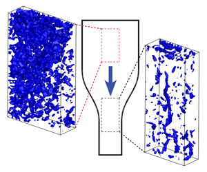
Figure 1. Sketch of the 2-D contraction used in our experiments, showing the coordinate axes used. Conceptual model of how a vortex tube aligned with the centreline stretches and amplifies as it moves through the contraction.
The early conceptual theory of Prandtl (Reference Prandtl1933) models turbulence as consisting of discrete vortex filaments aligned streamwise or perpendicular to the centreline, to explain its evolution though the contraction. The elongation of a vortical structure aligned with the axis of a contraction, schematically shown in figure 1, will enhance its vorticity and rotational speed, to conserve angular momentum. This predicts the streamwise velocity fluctuation reduces as the inverse of contraction ratio  $C$, while the lateral velocity fluctuations grow proportionally to $C^{1/2}$.
Taylor (Reference Taylor1935) used more general vorticity distributions to improve this modelling. He used a Lagrangian approach to obtain the amplification of the disturbance field at the exit of the contraction. He used one Fourier mode to represent vorticity disturbances in three-dimensional (3-D) cells (Taylor–Green vortices). Using Kelvin circulation theorem, he obtained different prefactors in the above theory assuming inviscid flow and rapid distortion. He showed that the streamwise velocity fluctuations reduce by a factor ranging between  $1/C$ and $2/C$. The variation in lateral velocity fluctuations obtained is the same as that of Prandtl’s except for the constants.
Ribner & Tucker (Reference Ribner and Tucker1952) performed more detailed spectral analysis of a random turbulent velocity field, deriving explicit relations for the fluctuations at the exit of the contraction. Similar expressions were obtained independently by Batchelor & Proudman (Reference Batchelor and Proudman1954). They did their analysis by assuming distortion of fluid elements to occur much faster relative to change in their position. They took into account a realistic and arbitrary distortion of isotropic turbulence. This theory was later dubbed rapid distortion theory (RDT), e.g. Sreenivasan & Narasimha (Reference Sreenivasan and Narasimha1978) and Hunt & Carruthers (Reference Hunt and Carruthers1990). In case of a symmetric contraction and  $C\geqslant 2$, they give an approximate ratio of energy of streamwise turbulent velocity outlet and inlet of the distortion as $(3/4)C^{-2}[\log (4C^{3})-1]$. Likewise, the ratio of the energy of the two lateral velocity components is approximately given as $(3/4)C$.
Early experiments on this configuration are those of Uberoi (Reference Uberoi1956). His wind-tunnel experiments investigated the effect of three different axisymmetric contraction ratios of  $C=4,9,16$, for a square cross-section duct. Nearly isotropic turbulence was achieved by passing through grids of various mesh sizes. The grid Reynolds numbers $Re_{M}=U_{i}M/\unicode[STIX]{x1D708}$ (where $U_{i}$ is the mean speed at the inlet of contraction and $M$ is the mesh size of the grid) are in the range 3700–12 000. Using hot-wires, he observed decreasing magnitude of the streamwise fluctuation, while the lateral fluctuations increase as the flow accelerates through the contraction. However, for the largest contraction ratio, of $C=16$, the streamwise fluctuations decrease initially, but then increase towards the exit, reaching higher values than at the inlet. These measurements are in disagreement with Prandtl’s theory, which he concluded applies only when $C<4$.
It is also observed that the linear theory (Ribner & Tucker Reference Ribner and Tucker1952; Batchelor & Proudman Reference Batchelor and Proudman1954) over-predicts the reduction of the streamwise component, while it over-predicts the increase in the lateral ones.
Hussain & Ramjee (Reference Hussain and Ramjee1976) studied the effect of an axisymmetric contraction, using four different contraction shapes but with the same contraction ratio of  $C\simeq 11$. They used essentially a high-speed air blower, with an outlet velocity of ${\sim}28~\text{m}~\text{s}^{-1}$. This produces an exit $Re\sim 10^{5}$ based on the nozzle diameter, while the turbulence is generated by a fine 1.4 mm mesh at $Re_{M}=234$. They found that the increase in the lateral turbulent kinetic energy is only half of that predicted from the linear theory. They also found an increase in the streamwise fluctuations when $C>4$.
Faced with these large discrepancies between the theories and the above-mentioned experiments, Tsugé (Reference Tsugé1984) modified the theoretical approach. He proposed that the smaller eddies agree better with linear theory than the larger ones, which are amplified by mean-flow inhomogeneities and grow for large contraction ratios, if  $C>4$. With these modifications he was able to closely reproduce the experimental results.
Han et al. (Reference Han, George and Hjärne2005) investigated (with correction for background disturbances) the budget of turbulent kinetic energy of grid-generated turbulence through an axisymmetric contraction with  $C\simeq 11$. In their following work (Reif et al. Reference Reif, George and Hjärne2005) they theoretically investigated this case, formulating a new definition of rapid distortion.
Ayyalasomayajula & Warhaft (Reference Ayyalasomayajula and Warhaft2006) experimentally investigated grid-generated turbulence subjected to mean strain using an axisymmetric contraction ( $4\,:\,1$) in a wind tunnel. They used both passive and active grids to generate a wide range of $Re_{\unicode[STIX]{x1D706}}$ (40–470) and by changing the mean wind speed, as high as $5~\text{m}~\text{s}^{-1}$. The evolution of turbulence statistics and return to isotropy after straining was studied using hot-wire measurements at mostly single points and were compared with predictions made using RDT. They observed that the effects of strain on small and large scales were different and give rise to nonlinear interactions. Following this work, Gylfason & Warhaft (Reference Gylfason and Warhaft2009) investigated the effect of axisymmetric strain on a passive scalar field. A transverse temperature gradient imposed on a homogeneous isotropic turbulence generated using passive and active grids ( $Re_{\unicode[STIX]{x1D706}}=50$ and 190 respectively) is passed through an axisymmetric contraction. A tensor model was developed to predict the evolution of the scalar and they suggest that this model can be applicable in straining regions when RDT is not accurate. The small-scale statistics deviated from RDT due to the nonlinearity neglected in RDT.
Chen et al. (Reference Chen, Meneveau and Katz2006) studied a different class of straining turbulent flow. Using planar particle image velocimetry (PIV), they measured the response of turbulence subjected to a planar straining–relaxation–destraining cycle in the framework of Reynolds averaged Navier–Stokes (RANS) and large eddy simulations (LES). The straining–destraining cycle was achieved by translating a piston in a water tank, in which turbulence was generated using four rotating active grids ( $Re_{\unicode[STIX]{x1D706}}=400$). The work mostly focused on the scale dependence of the RANS and LES variables, such as the Reynolds stress, subgrid-scale stress and dissipation.
However, recently, Ertunç & Durst (Reference Ertunç and Durst2008) have called into question the entire earlier experimental work which is based on using two-component  $\times$-configuration hot-wires. In a comprehensive study of the errors involved, they conclude that these measurements may be unreliable. This arises both from possible mass-flow-rate fluctuations in the wind tunnels, but primarily from electronic noise contamination of the hot-wire signals along with inadequate spatial resolution. These $\times$-wire probes are sensitive to the large accelerations of the mean flow and the accompanying reduction in important transverse length scales. Without correcting for these effects, they see discrepancies, near the exit of the nozzle, which reduce the transverse fluctuations by up to ${\sim}30\,\%$, while the longitudinal fluctuations become swamped by noise. They conclude that the observed anomalous increase in the longitudinal velocity fluctuations for large $C$ is a measurement artefact. Their careful experiments for a strong contraction with $C=14.75$ show continuous reduction in the streamwise fluctuations, until they have essentially disappeared.
On the other hand, not all studies have used hot-wires. Brown et al. (Reference Brown, Parsheh and Aidun2006) used two-component laser Doppler velocimetry (LDV) experiments to study the evolution of grid turbulence in a planar contraction between a linearly converging roof and ceiling, while the side walls were straight. They studied converging half-angles of  ${\sim}8^{\circ }$ giving $C(x_{1})$ up to 9 at the exit. With a water tunnel and a $M=9.5~\text{mm}$ square mesh grid they reached $Re_{M}=4500{-}9000$, with the corresponding $Re_{\unicode[STIX]{x1D706}}=51{-}99$, based on the Taylor microscale. Their pointwise LDV measurements show turbulence behaviour similar to that for the axisymmetric case, with streamwise velocity fluctuations decaying initially and then increasing. Using the local contraction ratio $C(x_{1})$ with the streamwise coordinate, the minimum is reached at $C\approx 2$, and this location is independent of $Re$ but depends on the inlet turbulence level. The flow reaches peak anisotropy between the various fluctuation components at $2.5<C<3.5$, but starts to return to isotropy at $C\approx 4$. LDV measurements are not subject to the same errors as hot-wire measurements. However, one could argue that this study uses a contraction that is too gradual to expect RDT to be fully applicable. The maximum value of the strain-rate parameter $S^{\ast }$ is 25 in our experiments.
The effects of a contraction on turbulent scalar fields have also been studied. Warhaft (Reference Warhaft1980) studied experimentally the decay of passive temperature fluctuations, with and without uniform straining. Thermal fluctuations were induced in grid-generated turbulence using a heated parallel array of fine wires, called the mandoline, and were subsequently strained by passing the flow through a  $C=4$ axisymmetric contraction. Using independent grids for the velocity and temperature fields, they could vary their length-scale ratios. The contraction was in all cases found to accelerates the thermal fluctuation decay. The streamwise velocity fluctuations decreased by a half and the transverse intensity increased by ${\sim}55\,\%$ (their figure 2), which is somewhat smaller than the predicted change.
Thoroddsen & Van Atta (Reference Thoroddsen and Van Atta1995a) also studied the effect of a 2-D contraction with  $C=2.5$ in a thermally stratified wind tunnel, with a strong linear temperature gradient. The reduction in the vertical height of the test section increases rapidly the mean temperature gradient and the strength of stable density stratification. This drastically reduces the vertical velocity fluctuations, while ‘fossilizing’ the temperature field. Without the temperature stratification, the streamwise root mean square reduces by ${\sim}40\,\%$ through the entire contraction, while the transverse component grows by a factor or ${\sim}30\,\%$, broadly consistent with the above study. Downstream of the exit these components approach the same level very slowly. The spectrum of the transverse fluctuations is greatly enhanced at the large-scale streamwise wavenumbers, when compared to the isotropic relations (their figure 10(a)). Thoroddsen & Van Atta (Reference Thoroddsen and Van Atta1995b) followed up by studying the turbulence in a constant-area vertical expansion. Iino et al. (Reference Iino, Van Atta and Keller2002) used a similar vertical contraction in the stratified tunnel, but now with a laterally expanding duct to keep the mean-flow velocity constant.
Direct numerical simulations (DNSs) can potentially provide time-resolved three-dimensional velocity and pressure fields, which are effective for deciphering the complete physics using not only point statistics, but also 3-D coherent structures and structure-based statistics. However, practical DNSs are currently limited to the modest  $Re_{\unicode[STIX]{x1D706}}\sim 200$. This is especially true in our configuration owing to the complexity of the boundary conditions.
Recently, Clay & Yeung (Reference Clay and Yeung2016) used DNS to reproduce the results of the experimental study by Ayyalasomayajula & Warhaft (Reference Ayyalasomayajula and Warhaft2006) with an axisymmetric contraction. Simulations up to a maximum  $Re_{\unicode[STIX]{x1D706}}$ of 95 were used to explain the mechanisms underlying the nonlinear interactions of different scales observed in the experiments. They used a time-dependent strain rate applied to the computational domain to closely match the experimental conditions. Homogeneous isotropic conditions were first obtained at a maximum $Re_{\unicode[STIX]{x1D706}}$ of 113, before starting the mean-straining simulations. A similar time-dependent strain rate in DNS was adopted previously by Gualtieri & Meneveau (Reference Gualtieri and Meneveau2010). They simulated the straining–destraining experiments by Chen et al. (Reference Chen, Meneveau and Katz2006) up to a maximum $Re_{\unicode[STIX]{x1D706}}$ of 40. Using the discriminant $\unicode[STIX]{x1D6E5}$ which combines the velocity gradient tensor invariants, they visualized vortical structures. The initial worm-like structures with arbitrary alignment (characterizing isotropy), tend to show a preferred alignment along the positive strain direction at the end of straining. On destraining, they tend to return back to the initial isotropic state.
Another notable numerical simulation is that of Jang et al. (Reference Jang, Sung and Krogstad2011) who tracked fully developed pipe flow through an axisymmetric contraction, and which largely focused on the boundary-layer structure. They also observed that turbulent kinetic energy, when scaled by the local velocity, decays rapidly in the core region. The coherent vortical structures were visualized based on the swirling strength from the DNS data. Spanwise vortical structures existing in the pipe are stretched into streamwise structures in the contraction, with only long ‘streaky’ structures aligned along the axis in the later part of it.
Other DNSs of strained turbulence include studies on: inertial particles dynamics in an axisymmetrically expanding homogeneous turbulent flow (Lee et al. Reference Lee, Gylfason, Perlekar and Toschi2015), homogeneous isotropic turbulence subjected to uniform plane strain (Zusi & Perot Reference Zusi and Perot2013) and axisymmetric contraction/expansion (Zusi & Perot Reference Zusi and Perot2014). Lee et al. (Reference Lee, Gylfason, Perlekar and Toschi2015) studied the dynamics of inertial-particle-laden turbulence subjected to axisymmetric expansion up to a maximum  $Re_{\unicode[STIX]{x1D706}}$ of 193 and for $S^{\ast }$ from 0.2 to 20. Under straining action, vorticity intensifies with the filaments (represented by isosurface of vorticity magnitude) aligning qualitatively with the extensional directions.
Based on the above survey of previous experimental studies, most work has been limited to single-point measurements using hot-wires or LDV, with varying degree of accuracy. None of these measurements provide any direct information on the vorticity in the flow, which is the conceptual underpinning of the basic theory. One can therefore argue that the time is ripe for applying the latest experimental techniques to this problem. Three-dimensional volumetric measurement techniques like tomographic particle image velocimetry (tomo-PIV) and shake-the-box (STB) particle-tracking techniques have now become available for this purpose (Elsinga et al. Reference Elsinga, Scarano, Wieneke and van Oudheusden2006; Schanz et al. Reference Schanz, Gesemann and Schröder2016). Furthermore, Casey et al. (Reference Casey, Sakakibara and Thoroddsen2013) introduced a new scanning laser-volume tomo-PIV technique to resolve a larger volume of the velocity field with good temporal and spatial resolutions. They applied this technique to the turbulence flow field in a round jet, tracking large coherent vortical structures. Ianiro et al. (Reference Ianiro, Lynch, Violato, Cardone and Scarano2018) most recently used three-camera tomo-PIV to study the vortical structures in a transitional swirling jet, at a  $Re$ of 1000. Westerweel et al. (Reference Westerweel, Elsinga and Adrian2013) have suggested a triple-pulse technique for more accurate tracking of particle trajectories.
In the current study, we have successfully employed such non-intrusive tomo-PIV/STB techniques. Using high-speed video cameras we obtain the first time-resolved measurements of coherent vortical structures within turbulent flow fields at various locations inside a 2-D planar contraction.
We use an active grid upstream of the contraction to enhance the turbulence level, thereby obtaining higher values of the turbulent  $Re_{\unicode[STIX]{x1D706}}\sim 250$. Active grids have become a common technique to achieve a higher level of turbulence in small-scale wind tunnels, since its introduction by Makita (Reference Makita1991), who reported turbulence with $Re_{\unicode[STIX]{x1D706}}\approx 400$ in his early wind-tunnel experiments. The active grid also gives us better control of the creation of large observable structures at the inlet to the contraction, compared to other canonical flows such as fully developed channel or pipe flow. Our laboratory facility does not allow for the set-up of a fully developed pipe or channel flow with such a large cross-section as 18 cm. Mydlarski (Reference Mydlarski2017) has comprehensively reviewed the subsequent developments to date. Recently, $Re_{\unicode[STIX]{x1D706}}$ of the order of $10^{3}$ has been achieved using active grids by Larssen & Devenport (Reference Larssen and Devenport2011), compared to $10^{2}$ for corresponding passive grids. The active grid consists of a square mesh of shafts with flaps/wings attached to them, where each shaft can be independently rotated about its axis. Even though active grids were initially used to study homogeneous, isotropic turbulence, they have now been employed to investigate a wider class of flows, such as an inhomogeneous shearless mixing layer between two homogeneous isotropic streams by Kang & Meneveau (Reference Kang and Meneveau2008) and in wind-tunnel models of atmospheric boundary layers by Michioka et al. (Reference Michioka, Sato and Sada2011). Thormann & Meneveau (Reference Thormann and Meneveau2015) extended this to shearless flow with a transverse linear gradient of turbulent kinetic energy. Active grids have also been applied to study the behaviour of air bubbles in a water channel using a vertical test section by Poorte & Biesheuvel (Reference Poorte and Biesheuvel2002) and Prakash et al. (Reference Prakash, Mercado, Wijngaarden, Mancilla, Tagawa, Lohse and Sun2016).
Other studies using active grids investigate: the effect of the flap shapes and holes in the flaps (Thormann & Meneveau Reference Thormann and Meneveau2014) with Hearst & Lavoie (Reference Hearst and Lavoie2015) reporting that solid flaps with no holes generate higher turbulent intensities and  $Re_{\unicode[STIX]{x1D706}}$, turbulent boundary layers (Sharp et al. Reference Sharp, Neuscamman and Warhaft2009; Dogan et al. Reference Dogan, Hanson and Ganapathisubramani2016, Reference Dogan, Hearst and Ganapathisubramani2017; Hearst et al. Reference Hearst, Dogan and Ganapathisubramani2018), turbulent wakes (Hearst et al. Reference Hearst, Gomit and Ganapathisubramani2016) and particle clustering (Obligado et al. Reference Obligado, Teitelbaum, Cartellier, Mininni and Bourgoin2014, Reference Obligado, Cartellier and Bourgoin2015). Such grids have also been used in more applied studies on wind turbines and wind farm models (Cal et al. Reference Cal, Lebrón, Castillo, Kang and Meneveau2010; Bossuyt et al. Reference Bossuyt, Howland, Meneveau and Meyers2017; Hearst & Ganapathisubramani Reference Hearst and Ganapathisubramani2017; Rockel et al. Reference Rockel, Peinke, Hölling and Cal2017). Thoroddsen & Van Atta (Reference Thoroddsen and Van Atta1993) also investigated the effect of a fixed grid configuration on thermally stratified turbulence, comparing bi-planar square grids to horizontal or vertical rods, and showed that the horizontal rods produced von Kármán vortex streets which are only visible in the spectra up to $x/M\sim 30$, but absent for the bi-planar grids.

Figure 2. (a) Schematic of the gravity-driven water tunnel with the 2-D contraction. An extensional part was added for some experiments to increase the distance between the active grid and the entrance to the contraction which is either 238 mm or 478 mm. (b) Measurement regions illustrated with respect to the coordinate axis positioned at the start of contraction (SOC). EOC denotes the end of contraction. Here  $x_{AG}$ represent the distance from the bottom shaft of the active grid. $x_{AG}$ (Ext) gives the distance from the active grid with the extension added. See supplementary material § S1 for photographs, available online at https://doi.org/10.1017/jfm.2019.887.
2 Experimental set-up
2.1 Constant-head vertical water tunnel with a 2-D contraction
We study turbulence in a constant-head vertical water tunnel with a 2-D contraction, i.e. the square inlet is contracted in one of the horizontal directions. Figure 2(a) shows the acrylic tunnel which consists of an overhead tank, a straight vertical inlet duct of cross-section  $260\times 260~\text{mm}$, the active grid module, a 2-D contraction and a bottom straight section. Background turbulence in the inlet flow is suppressed, first by passing it through a wound mesh inside the outer part of the overhead tank, followed by two perforated steel plates and a metallic honeycomb placed in the straight section. Flow is then guided smoothly into the active grid module through a 203 mm long converging section which reduces the cross-section to $180\times 180~\text{mm}$. The active grid module is described in detail in the next subsection. The water passes through a 238 mm long straight section after leaving the grid (measured from the bottom grid shaft) before entering the contraction. The contraction ratio is $2.5\,:\,1$, reducing the cross-section from $180\times 180~\text{mm}$ to $72\times 180~\text{mm}$. The length of the contraction is equal to its inlet dimension of 180 mm. The contraction profile (in mm) is given by the equation,
 $$\begin{eqnarray}y=\frac{1}{2}\left\{180{-}108\left[6\left(\frac{x}{180}\right)^{5}-15\left(\frac{x}{180}\right)^{4}+10\left(\frac{x}{180}\right)^{3}\right]\right\}.\end{eqnarray}$$
This fifth-order polynomial is expressed in the current coordinate system, and ensures that the contraction is free of flow separation and provides flow uniformity (Bell & Mehta Reference Bell and Mehta1988). The actual profile of the contraction in 3-D perspective is sketched in figure 1. The contraction profile is machined out of an acrylic block and is placed between two glass plates to form the contracting stream. Glass plates provide better optical access for the imaging and are more resistant to scratching than the acrylic. To ensure that there are minimal effects from the exit boundaries, a 500 mm long straight section of the same cross-section is provided downstream of the end of the contraction. Two horizontal outlet pipes extend symmetrically from the sides.
Constant head is maintained by supplying water from a 500 l sump to the overhead tank using a centrifugal pump (maximum rating of 600 lpm at 10 m head). The flow rate through the tunnel and thus the level in the overhead tank is controlled using three ball valves – one valve at the pump suction and one valve each in the two return lines from the exit of the tunnel. The inlet valve was set to approximately  $0.28~\text{m}~\text{s}^{-1}$ measured at the level following the grid. In all experiments, the return-line valves are kept fully open to achieve maximum flow rate. To eliminate bubbles from the flow, the vertical tunnel is initially filled up to the brim from the bottom before the start of experiments. Flow is then set with the main centrifugal pump, maintaining a constant level in the overhead tank by adjusting the bypass valve. All measurements are performed at least 5 min after a steady flow is achieved through the loop. Experiments are conducted near the room temperature of $21\,^{\circ }\text{C}$, giving water a density of $\unicode[STIX]{x1D70C}=998~\text{kg}~\text{m}^{-3}$ and dynamic viscosity of $\unicode[STIX]{x1D707}=9.79\times 10^{-4}~\text{Pa}~\text{s}$.

Figure 3. Sketch of the active grid showing only  $3\times 3$ shafts in the grid assembly (left), and a closer view of the attachment of flaps to the shaft (right). Photographs of the active grid can be found in § S1.
2.2 The active grid
The active grid, shown in figure 3, enhances turbulence in the flow by rotating numerous small flaps within the uniform inlet stream. The assembly consists of 10 rotating stainless steel shafts of diameter 6.35 mm with a grid spacing of  $M=30~\text{mm}$. Each shaft has six square flaps ( $20\times 20\times 0.5~\text{mm}$) with two 6 mm through holes, which reduce its solidity and inertia. To improve flow homogeneity across the span of the test section, half-flaps without holes are attached to the side walls of the channel. The shafts are oriented in two perpendicular directions and are confined to two horizontal planes vertically separated by 9 mm. Shafts in the top and bottom planes are shown in red and black respectively in figure 3. A dual-shaft stepper motor (ISM-7401D NEMA-23 from National Instruments) controls each shaft separately, enabling independent rotation. We use rubber-sealed stainless steel deep-groove ball bearings to support the shafts through the tunnel walls, with V-rings for good sealing. Stainless steel circlips mounted on the end of the shafts arrest axial movement. We use the NI cRIO-9035 industrial-grade embedded controller with two NI 9375 Digital I/O modules (each module has 16 DI and 16 DO channels) for precise control of the motor rotation, which spins at $N=3~\text{rps}$ (Rossby number, $Ro=2\langle U_{in}\rangle /M\unicode[STIX]{x1D6FA}\approx 0.95$, where $\unicode[STIX]{x1D6FA}=2\unicode[STIX]{x03C0}N$) in all our experiments. More details of the control system can be found in Mugundhan (Reference Mugundhan2019). A proximity sensor sets the initial position of the flaps to the horizontal (‘home’ position) at the start of rotation cycle, which enables synchronous rotation.
The active grid can be operated using many different rotation protocols, broadly classified into two modes – synchronous (sync) and random. In the synchronous mode, the angles of all flaps are coordinated in sync with each other, whereas in the random mode, the direction of rotation of each shaft changes randomly. Mydlarski & Warhaft (Reference Mydlarski and Warhaft1996) report in their wind-tunnel experiments, that they get higher values of  $Re_{\unicode[STIX]{x1D706}}$ with an active grid when it is operated in the random mode. The synchronous rotation has four modes of operation – S1–S4, as illustrated in figure 4, which shows a schematic of the grid from the top. In modes S1 and S2 all shafts rotate in sync in the specified directions, whereas in modes S3 and S4, shafts in the top plane remain open for the entire cycle, i.e. oriented vertically, and only the bottom shafts rotate. We chose mode S1 as our base case as it injects circulation of opposite sign into the flow, while mode S2 preferably injects circulation of the same sign into the flow. The different rotation modes show the generality of our results, even for the ‘pathological’ rotation protocols S2 and S4, but we focus mostly on the base mode S1.

Figure 4. Shaft protocols for different synchronous modes of the active grid. (a) Sync mode 1 (S1) – counter-rotating adjacent rods in both planes; (b) sync mode 2 (S2) – all rods rotated in same direction; (c) sync mode 3 (S3) – counter-rotating adjacent rods in bottom plane only, while the top flaps are open; (d) sync mode 4 (S4) – rods in the bottom plane rotated in same direction. In modes S3 and S4, rods in the top plane are fixed with flaps aligned vertically. A: anticlockwise; C: clockwise; O: open. M1–M10 represent the motors connected to each shaft (M1, M2, M3, M6, M7 are in the bottom plane and M4, M5, M8, M9, M10 in the top plane). Directions are specified when viewed in the negative  $y$ and $z$ directions.
In the random mode (R), the direction of rotation of the shafts changes randomly, while keeping a constant rotation speed of 3 rps, which is called the single random mode in the literature (Poorte & Biesheuvel Reference Poorte and Biesheuvel2002). The cruise time also varies randomly between the period of  $180^{\circ }$ and $540^{\circ }$ of a rotation. This sets the average cruise time equal to the period of one complete revolution. In the so-called double random mode, the speed of each shaft is also a random variable. However we implement only the single-random mode as it is common in the literature. Also, Larssen & Devenport (Reference Larssen and Devenport2011) conclude from their study with the double random mode that the mean rotation speed has a greater effect on $Re_{\unicode[STIX]{x1D706}}$ than the deviation of cruise time and rotation rate.

Figure 5. Schematic view of the test section with laser illumination (green), volume optics and four high-speed video cameras. (a) Shows the front view and (b) shows the top view.
2.3 Illumination and imaging set-up
Figure 5 shows a schematic of the illumination and imaging system in relation to the contraction used in our experiments. The cameras are sketched in the top view only and are arranged in a horizontal plane. A LaVision tomo-PIV imaging system is used to obtain time-resolved 3-D measurements of the volumetric flow field. We use both LaVision’s tomo-PIV (Elsinga et al. Reference Elsinga, Scarano, Wieneke and van Oudheusden2006) and PTV algorithms (Schanz et al. Reference Schanz, Gesemann and Schröder2016), to compute velocity fields from the captured particle images. Particles are illuminated using a dual-cavity pulsed Nd-YLF, 527 nm green laser (Litron LDY 300 PIV) with a maximum output of  $23~\text{mJ}~\text{pulse}^{-1}$ (at 70 % power and a frequency of 1 or 1.3 kHz) and of pulse width 100 ns. In our experiments both of the lasers are flashed together with no separation time to obtain a sufficiently high illumination intensity.
LaVision volume optics (modules A and B reference number 1108676) are used to expand the laser beam into a volume slice. The volume optics consist of a focusing lens and two perpendicular cylindrical lenses which expand the beam to illuminate a 3-D volume in the measurement region, as shown in figure 5. A metallic aperture cuts off the dim edges of the expanded laser, forming a measurement region that is approximately  $56\times 106\times 20~\text{mm}$, as indicated in figure 2(b).
The flow evolution is tracked in three separate experimental regions in runs on separate days. The first region is close to the grid, before the flow enters the contraction. The second is inside the contraction and the third is at the bottom of the contraction, which includes its exit and the following straight section. These regions are marked as P1, P2 and P3 in figure 2(b). An overlap of positions P2 and P3 is used to check for consistency of the statistics between the separate experimental runs.
Imaging is done using four high-speed video cameras (LaVision Imager Pro HS) with Scheimpflug attachments and 105 mm Nikkor lenses at an aperture of  $f/16$. They allow frame rates up to 1279 fps at full 4 Mpx resolution. Two cameras are placed on either side of the measurement zone, as shown in figure 5. Images are captured with a resolution of $1152\times 2016~\text{px}$ at 1000 fps. However, in position P3 at the exit of contraction, where the mean flow has accelerated, a higher frame rate of 1300 fps is used. The LaVision control unit synchronizes the cameras and the laser providing one laser flash per frame. For good reconstruction quality, we maintain optimum angles between the cameras, and those viewing from opposite sides are positioned so that they do not have co-linear lines of sight. For positions P1 and P2 the angles between C1/C2 and C3/C4 are $30^{\circ }$ and $38^{\circ }$ respectively, while for the narrower tunnel in P3 they are $24^{\circ }$ and $32^{\circ }$. In P2, cameras C1, C2, C3, C4 make angles $105^{\circ }$, $75^{\circ }$, $71^{\circ }$ and $109^{\circ }$ with the laser respectively.
2.4 Calibration and seeding particles
Spatial calibration was accomplished using an 11.8 mm thick 4-plane calibration plate from LaVision (Number: 106-10) with two different depths of white dots on a black background per side. The edges of the calibration plate have been cutoff to fit into the test section, where it is mounted on a support rod extending from the bottom of the tunnel. The test section is filled with water and calibration images are taken with the plate in the centre of the volume. The calibration images are taken under normal laboratory lighting and third-order mapping polynomials in the image plane are obtained using the LaVision DaVis software.
Both the tomo-PIV and STB algorithms require a second volume self-calibration step (Weineke Reference Weineke2008) which is used to improve the original calibration using the actual particle images. In self-calibration, we use pre-processed images (pre-processing involves subtracting a sliding minimum over 5 px, normalizing with a local average, Gaussian smoothing and sharpening of the raw images) to compute disparity vectors for each sub-volume of the measurement region, which are then used to correct the original calibration. Volume self-calibration is done using the 20 000 highest-intensity particles, by dividing the measurement zone into  $5\times 5\times 3$ sub-volumes with a maximum allowed triangulation error between 1.8 and 2.0 pixel. The procedure is repeated, updating the corrections to the mapping functions after every step until the standard deviation of the fit falls from ${\sim}0.5~\text{pixels}$ to below 0.1 pixels. Volume self-calibration accounts for any misalignments such as slight changes in the positions of the cameras and other optical disturbances during conduct of the experiment.
For seeding particles we use fluorescent red or orange polyethylene microspheres with diameters in the range  $63{-}106~\unicode[STIX]{x03BC}\text{m}$ which are close to neutrally buoyant with a density of $1.05~\text{g}~\text{cm}^{-3}$ (from Cospheric). To avoid particle agglomeration and to allow reuse of the particles, they are first treated with diluted Tween-80 surfactant solution. To ascertain the ability of the particles to faithfully follow the fluid flow, we estimate the time constant governing their dynamics. Using the mean particle diameter and assuming a low- $Re$ Stokesian drag coefficient of 1, based on Adrian & Westerweel (Reference Adrian and Westerweel2011), we estimate the particle time constant in our case as ${\sim}20~\unicode[STIX]{x03BC}\text{s}$. This corresponds to a Stokes number of $2\times 10^{-4}$, indicating minimal lag between the flow and tracer.
2.5 Time-resolved tomo-PIV and STB particle tracking algorithms
To obtain velocity fields we use two separate techniques: tomo-PIV and STB. In the tomo-PIV analysis, 3-D reconstruction is done with the FastMART algorithm in DaVis (version 8.2.2). The algorithm consists of initialization with the single-step MLOS (multiplicative line-of-sight) algorithm (Worth & Nickels Reference Worth and Nickels2008; Atkinson & Soria Reference Atkinson and Soria2009) with subsequent calculations using the MART (multiplicative algebraic reconstruction) (Elsinga et al. Reference Elsinga, Scarano, Wieneke and van Oudheusden2006) and SMART (simultaneous MART) (Atkinson & Soria Reference Atkinson and Soria2009) algorithms. The direct correlation technique with binning is used for the 3-D velocity calculations. The region with S-N (signal-noise) ratio greater than 2 is used for the cross-correlation, which determines the depth of the volume reconstruction. Here, S-N is calculated by the ratio of the intensities of true particles to that of ghost intensities. However, tomo-PIV suffers from some disadvantages, such as the occurrence of ghost particles, which decreases the accuracy of the method. Spatial averages of interrogation volumes are employed during correlation, which smooth velocity gradients and fine structures. Furthermore, volume reconstructions are needed at every time step, which are much more computationally demanding than particle tracking.
STB is a new 4-D Lagrangian particle-tracking velocity measurement technique that can handle densely seeded flows while producing a minimum number of ghost particles (Schanz et al. Reference Schanz, Schröder, Gesemann, Michaelis and Weineke2013a, Reference Schanz, Gesemann and Schröder2016). It brings together volume self-calibration, optical transfer function features of tomo-PIV (Schanz et al. Reference Schanz, Gesemann, Schröder, Weineke and Novara2013b) and iterative triangulation and the image matching of the iterative reconstruction of volume particle distribution (IPR), introduced by Weineke (Reference Weineke2013). Particle velocities obtained from from the tracks are then mapped to a three-dimensional Eulerian grid (Gesemann Reference Gesemann2015). Lagrangian particle-tracking methods can typically handle a seeding density one order smaller than those in tomo-PIV, i.e. only  $\simeq 0.005~\text{ppp}$. The ‘image matching’ technique used in IPR enables 3-D reconstructions as accurate as tomo-PIV with seeding densities as high as 0.05 ppp. On the other hand, keep in mind that 5–10 particles are needed in each interrogation volume for the correlation method, equalizing the total number of velocity vectors obtained in the two techniques.
We compare the processing results of these two algorithms in supplementary material § S2 and find that both produce similar results for the coherent vortical structures. As STB can now produce a similar density of velocity vectors to tomo-PIV, reduces ghost particles and greatly reduces the processing time we present the results processed using STB from DaVis (version 8.4.0) from LaVision in this paper. Most results presented herein are from STB calculations, with typically 30 000 particle tracks appearing in the volume. Pre-processing of images for STB is the same as for tomo-PIV except that no smoothing or sharpening is applied. For the pointwise statistics, a grid of either 36 or 48 pixels with time filter length of five time steps is used, while for structure-based statistics we use 11 time steps to improve traceability of the coherent structures. Details of the velocity grids and the convergence of flow features with spatial resolution are presented in the supplementary material § S2.

Figure 6. (a) Joint probability density function (PDF) of parameters  $\unicode[STIX]{x0394}V/\unicode[STIX]{x0394}y$ and $-(\unicode[STIX]{x0394}U/\unicode[STIX]{x0394}x+\unicode[STIX]{x0394}W/\unicode[STIX]{x0394}z)$ for volume size of $4W$, contours shown for the range 0.01–0.04. (b) PDF for $\unicode[STIX]{x1D709}$. All plots shown for the grid of size 48 voxels.
To evaluate the quality of the STB velocity computation for a chosen grid resolution, we use methods adopted in Zhang et al. (Reference Zhang, Tao and Katz1997) and Casey et al. (Reference Casey, Sakakibara and Thoroddsen2013), wherein they analyse the residual of the continuity equation to evaluate the quality of their tomo-PIV computations. The three terms of the continuity equation are computed over a cuboidal volume of sizes  $W$,
$W$,  $2W$ and $4W$ by taking differences of velocities averaged over opposite faces (as seen in Zhang et al. (Reference Zhang, Tao and Katz1997)). We use the STB velocities computed on a grid of 48 pixels with a filter of 11 time steps for region P2 for this equality evaluation. Thus, here, $W$ is taken as 48 pixels. Figure 6(a) shows the contour plot of joint probability density function (PDF) of $\unicode[STIX]{x0394}V/\unicode[STIX]{x0394}y$ and $-(\unicode[STIX]{x0394}U/\unicode[STIX]{x0394}x+\unicode[STIX]{x0394}W/\unicode[STIX]{x0394}z)$, for case $4W$. Here $U$,
$U$,  $V$,
$V$,  $W$ represent the instantaneous velocities averaged over the faces. The $45^{\circ }$ line on the plot corresponds to the divergence-free velocity field, and it is seen that our data align along this line with small scatter, indicating that the divergence errors are acceptable. The peak value of the contours is shifted to the left of zero, as the flow accelerates through the contraction. Correlation coefficient between the two quantities plotted is calculated to be 0.91. This is as expected based on the values of 0.82 and 0.96 reported by Ganapathisubramani et al. (Reference Ganapathisubramani, Lakshminarasimhan and Clemens2007) and Casey et al. (Reference Casey, Sakakibara and Thoroddsen2013) respectively, for their calculations in a turbulent jet, with similar spatial resolutions. With the higher-magnification experiments (see § 3.10) we get a higher correlation coefficient of 0.94, for the same volume size. This is shown in the supplementary figure S14.
Deviation of the velocity field from divergence-free data is also represented by a non-dimensional parameter defined as (Zhang et al. Reference Zhang, Tao and Katz1997),
 $$\begin{eqnarray}\unicode[STIX]{x1D709}=\frac{(\unicode[STIX]{x2202}U/\unicode[STIX]{x2202}x+\unicode[STIX]{x2202}V/\unicode[STIX]{x2202}y+\unicode[STIX]{x2202}W/\unicode[STIX]{x2202}z)^{2}}{(\unicode[STIX]{x2202}U/\unicode[STIX]{x2202}x)^{2}+(\unicode[STIX]{x2202}V/\unicode[STIX]{x2202}y)^{2}+(\unicode[STIX]{x2202}W/\unicode[STIX]{x2202}z)^{2}}.\end{eqnarray}$$
 The parameter  $\unicode[STIX]{x1D709}$ varies between zero and 1, and deviation from 0 represents the normalized deviation from the divergence-free condition. Figure 6(b) shows the PDF for $\unicode[STIX]{x1D709}$ for all three volume sizes. The mean values of $\unicode[STIX]{x1D709}$ are 0.21, 0.15 and 0.06 for $W$,
$W$,  $2W$ and $4W$ respectively. The corresponding values reported by Casey et al. (Reference Casey, Sakakibara and Thoroddsen2013) are similar at 0.36, 0.19 and 0.09 for their highest $Re$ case. Our results show slightly better closure of continuity despite our higher $Re_{\unicode[STIX]{x1D706}}$ and less resolved Kolmogorov scales. The closure is even better in our higher-magnification experiments discussed in supplementary material § S7.
3 Results
We present the results of the experiments described above in the following manner. First, in § 3.1 we show characteristic turbulent parameters of the flow at specific points to give a basic sense of the turbulence level and behaviour in the channel. Next, in § 3.2 we discuss the mean velocity and the effect of the active grid rotation on the homogeneity of the flow. We then examine the evolution of the fluctuating velocity (§ 3.3) and vorticity statistics (§ 3.4) through the contraction. With this ground work we delve into a discussion on coherent vortical structures (§ 3.5) and investigate the alignment of vorticity with the principal strain-rate directions (§ 3.6) and the orientation of the vorticity vector (§ 3.7) and coherent structures (§ 3.8) in the streamwise direction. We then solidify the validity and broader applicability of our findings by briefly presenting additional experiments in which we improve the homogeneity of the flow with a larger distance between the active grid and SOC, showing little change in the results (§ 3.9), and increase the magnification of the cameras to resolve smaller scales (§ 3.10). All results presented are based on STB calculations unless otherwise stated.
3.1 Turbulence parameters
The important turbulent parameters computed at two different downstream locations are tabulated in table 1. Point A is located 125 mm ( $x=-113~\text{mm}$) downstream of the active grid still inside the straight section and point B is located at 30 mm ( $x=30~\text{mm}$) inside the start of the contraction. These points lie on the centreline of the tunnel. The mean streamwise velocity in the straight inlet section varied between 0.27 and $0.28~\text{m}~\text{s}^{-1}$ in our experiments. Turbulence intensities after the active grid are initially high, then decay along the flow direction, as expected. Higher values of fluctuations at point A are observed in modes S1, S3 and R, with the highest of 16.9 % obtained in the random mode. This point is located on the centreline of the tunnel at 125 mm ( $x=-113~\text{mm}$, $x_{AG}/M=4.2$) from the active grid. In modes S2 and S4, where shafts rotate in the same direction, lower turbulence intensities are obtained. This trend is also noted for the turbulent Reynolds number based on the Taylor microscale, $Re_{\unicode[STIX]{x1D706}}$, at both of the points. The highest value of $Re_{\unicode[STIX]{x1D706}}=292$ is achieved at point A in the random mode, which then reduces to 231 at point B. The value of $Re_{\unicode[STIX]{x1D706}}$ initially reduces in the straight section, due to the decay of the velocity fluctuations, while the Taylor microscale remains approximately a constant. There is some increase in $\unicode[STIX]{x1D706}$, as the flow enters the contraction, which results in higher values of $Re_{\unicode[STIX]{x1D706}}$.
Table 1. Flow parameters at location  $x=-113~\text{mm}$ ( $x_{AG}/M=4.2$) upstream of the start of the contraction (top), at $x=30~\text{mm}$ ( $x_{AG}/M=8.9$), which is slightly inside the contraction (middle), and at $x=30~\text{mm}$ ( $x_{AG}/M=16.9$) with the extensional part (bottom).

Turbulence kinetic energy is computed as  $k=(u_{rms}^{2}+v_{rms}^{2}+w_{rms}^{2})/2$, based on the root mean square of the fluctuating velocity components. The dissipation rate is approximated by,
 $$\begin{eqnarray}\unicode[STIX]{x1D700}=15\unicode[STIX]{x1D708}\left\langle \!\left(\frac{\unicode[STIX]{x2202}u}{\unicode[STIX]{x2202}x}\right)^{2}\right\rangle .\end{eqnarray}$$
 The notation is the following: the instantaneous velocity  $U=\langle U\rangle +u$, $V=\langle V\rangle +v$, $W=\langle W\rangle +w$, where $\langle U\rangle$, $\langle V\rangle$ and $\langle W\rangle$ are the time averaged velocities and, $u$,
$u$,  $v$ and $w$ denote the fluctuations. Equation (3.1) assumes homogeneity and local isotropy. Sirivat & Warhaft (Reference Sirivat and Warhaft1983) showed for grid turbulence that the estimate of $\unicode[STIX]{x1D700}$ using (3.1) agrees well with that computed by two other approaches: differentiation of the energy decay and integration of the velocity spectrum. Brown et al. (Reference Brown, Parsheh and Aidun2006) also use (3.1), showing that the dissipation rate agrees well with other estimates even though their flow is not isotropic. We also compare the isotropic estimate of $\unicode[STIX]{x1D700}$ to a more complete expression of $\langle s_{ij}s_{ij}\rangle$ in our high-magnification experiments, which are described in the supplementary material § S7.
The length scales associated with the turbulence are computed using the spatial auto-correlation of the streamwise velocity (Pope Reference Pope2000). For homogeneous turbulence, the correlation of streamwise velocities at two points axially separated by a distance  $r$ is given by,
 $$\begin{eqnarray}f(r)=\frac{\langle u(x)u(x+\boldsymbol{e}_{\boldsymbol{x}}r)\rangle }{\langle u^{2}\rangle }.\end{eqnarray}$$
 The integral length scale  $L$ and Taylor microscale $\unicode[STIX]{x1D706}$, are computed using the spatial correlation function $f$ as
 $$\begin{eqnarray}L=\int _{0}^{\infty }f(r)\,\text{d}r,\quad \unicode[STIX]{x1D706}=\left(-{\textstyle \frac{1}{2}}f^{\prime \prime }(0)\right)^{-1/2}.\end{eqnarray}$$
 The variation of the correlation  $f$ is shown for modes S1 and R in the supplementary figure S16. In both cases the curve reaches zero, where we stop the integration. The Reynolds numbers based on these length scales, presented in table 1, are defined as, $Re_{L}=k^{1/2}L/\unicode[STIX]{x1D708}$ and $Re_{\unicode[STIX]{x1D706}}=k^{1/2}\unicode[STIX]{x1D706}/\unicode[STIX]{x1D708}$. In case of isotropic flows, the Taylor microscale is often estimated as $\sqrt{u^{2}/\left\langle \left(\unicode[STIX]{x2202}u/\unicode[STIX]{x2202}x\right)^{2}\right\rangle }$ (Pope Reference Pope2000), which would give slightly smaller values for $Re_{\unicode[STIX]{x1D706}}$. If we apply this estimate to our data, the largest of our $Re_{\unicode[STIX]{x1D706}}$, which occurs for the random mode, reduces from 292 to 244. The smaller Kolmogorov length scale is computed as $\unicode[STIX]{x1D702}=(\unicode[STIX]{x1D708}^{3}/\unicode[STIX]{x1D700})^{1/4}$. The velocity grid resolution including the 75 % overlap is given by $\unicode[STIX]{x1D6FF}$ and is compared in table 1.
The turbulence-to-mean-strain time ratio is defined as  $S^{\ast }=Sk/\unicode[STIX]{x1D700}$ (Lee & Reynolds Reference Lee and Reynolds1985; Pope Reference Pope2000; Ayyalasomayajula & Warhaft Reference Ayyalasomayajula and Warhaft2006), where $S$ is the mean strain rate. Here, we use the dominant extensional strain rate ( $2\unicode[STIX]{x2202}\langle U\rangle /\unicode[STIX]{x2202}x$) for the mean strain rate $S$. The value of $S^{\ast }$ should be very large to apply rapid distortion theory. (Ayyalasomayajula & Warhaft Reference Ayyalasomayajula and Warhaft2006). For their flows, $S^{\ast }$ varied between 10 and 100. However, as they study an axisymmetric contraction they use a different prefactor ( $\sqrt{3}$) to calculate the mean strain.

Figure 7. (a) Streamwise evolution of the mean streamwise velocity  $\langle U\rangle$, on the centreline, for different oscillation modes of the active grid: synchronous modes S1–S4 and random mode R. The streamwise velocity is normalized by the area averaged mean inlet velocity in the straight section, $\langle U_{in}\rangle$. Vertical black lines mark the start and end of the contraction. Transverse profiles of mean streamwise velocity $\langle U\rangle (y)$ at different $x$ locations for mode S1 (b) and mode R (c). Locations $x=-90~\text{mm}$ and $x=-30~\text{mm}$ are before the entrance to the contraction. They correspond to $x_{AG}/M\approx 5$, 7, 9 and 11, where $x_{AG}$ is the distance from the bottom shafts of the active grid. The streamwise velocities in (b) and (c) are normalized by the local area averaged velocity at the corresponding $x$-location, $\langle U_{lm}\rangle$.

Figure 8. (a) Streamwise variation of the normalized mean strain  $\unicode[STIX]{x2202}\langle U\rangle /\unicode[STIX]{x2202}x$ for different modes. (b) Streamwise variation of $S^{\ast }$ for grid-rotation modes S1 and R. Vertical black lines mark the start and end of the contraction. The vertical red line marks the maximum curvature location.
3.2 Mean velocity
Figure 7(a) shows the mean streamwise velocity  $\langle U\rangle$ on the centreline of the tunnel. The values have been time averaged over 4.2 s (this corresponds to ${\approx}8\unicode[STIX]{x1D70F}$, where $\unicode[STIX]{x1D70F}$ is the eddy turnover time computed based on the integral length scale and the fluctuation at the start of contraction), and comparison between four realizations confirms good convergence. Velocity is normalized by the corresponding mean inlet velocity $\langle U_{in}\rangle$ in the straight channel averaged over the $y$ direction. The mean velocity in our experiments varies in the range $0.27{-}0.28~\text{m}~\text{s}^{-1}$. The flow accelerates inside the contraction and the measured mean streamwise values match closely the local cross-sectional area ratio, the outlet speed reaching 2.5 times the inlet velocity. There are minor differences seen between the different grid-rotation modes in the initial straight section and into the first part of the contraction (figure 7(a)). This is due to the flow not being entirely uniform in the transverse direction, both from the periodicity of the grid and the nature of the contracting geometry. We quantify the errors in the mean and root mean square (r.m.s.) quantities and discuss the convergence of our results in the supplementary material sections § S3 and S4 respectively.
The transverse profile of  $\langle U\rangle$ for modes S1 and R is shown in figures 7(b) and 7(c) respectively. The profiles are shown at four locations, $x=-90$, $-30$, $30$ and $90$ mm, corresponding to $x_{AG}/M\approx 5$, 7, 9 and 11, where $x_{AG}$ is the distance from the bottom shafts of the active grid. Velocity profiles have been normalized by the local mean velocity $\langle U_{lm}\rangle$ averaged over the transverse $y$ direction. For mode S1 a strong signature of the shaft rotation can be seen in the velocity profile at $x=-90~\text{mm}$. The non-uniformity reduces with the vigorous turbulent transport of momentum in the transverse direction, as we move further downstream. However, the flow still remains slightly non-uniform for mode S1 when it enters the contraction. These profiles are much more uniform in the case of the random mode. We present additional information how the active grid rotation influences the homogeneity of the flow for the different rotation modes in the supplementary material § S5.
An important parameter in strained turbulence is the strain-rate parameter, which is defined above. The streamwise variations of the mean strain rate and the strain-rate parameter  $S^{\ast }$ are shown in figures 8(a) and 8(b) respectively. We plot $S^{\ast }$ for the modes S1 and R which have the highest turbulent fluctuations. The maximum value of $S^{\ast }$ is approximately 25.

Figure 9. Streamwise variation of velocity and vorticity r.m.s. along the centreline. (a) Streamwise velocity  $u_{rms}$; (b) transverse velocity $v_{rms}$; and (c) spanwise velocity $w_{rms}$ for different modes of the active grid, i.e. the four synchronous modes S1–S4 and the random mode R. Streamwise evolution of the vorticity r.m.s. of (d) streamwise vorticity $\unicode[STIX]{x1D714}_{x,rms}$; (e) transverse vorticity $\unicode[STIX]{x1D714}_{y,rms}$; and (f) spanwise vorticity $\unicode[STIX]{x1D714}_{z,rms}$, for different modes of the active grid. Here, $\langle U_{in}\rangle$ is the area averaged mean inlet velocity in the straight section. The vertical black lines represent the start and end of the contraction. The vertical red line marks the maximum curvature location.
3.3 Fluctuating velocity statistics
Figure 9(a–c) shows the streamwise variation of the r.m.s. velocities  $u_{rms}$, $v_{rms}$ and $w_{rms}$ on the centre of the tunnel. They are normalized by the mean velocity $\langle U_{in}\rangle$ in the straight section. There is a slight discontinuity seen in the profiles within the contraction, as measurements at positions P2 and P3 are from different experimental realizations taken on different days. However, the trends seen for $u_{rms}$ and $v_{rms}$ in the contraction are as expected from the literature. All r.m.s. fluctuations decay rapidly in the straight section, but in the contraction, $u_{rms}$ continues to decay whereas there is an increase in the transverse components $v_{rms}$ and $w_{rms}$. In wind-tunnel experiments with planar contraction of $C=2.5$, the same as the current study, Thoroddsen & Van Atta (Reference Thoroddsen and Van Atta1995a) also observed decay in the $u_{rms}$ and increase in $v_{rms}$. These trends are similar to that proposed in Prandtl’s theory for an axisymmetric contraction (Prandtl Reference Prandtl1933). According to his theory, streamwise velocity fluctuations vary as inverse of $C$ and lateral fluctuations grow proportionally to $C^{1/2}$. This behaviour has been verified experimentally by Uberoi (Reference Uberoi1956) in his experiments with an axisymmetric square contraction and he concludes Prandtl’s theory holds good when $C<$4, which is true in our case. The decay in $u_{rms}$ in our current results is proportional to $1/C$, but the increase in $v_{rms}$ is not proportional to $C^{1/2}$, its increase is weaker.
The spanwise  $w_{rms}$ relatively has higher values in region P1 and shows a decay upstream of the contraction. In the contraction, similar to the transverse $v_{rms}$, $w_{rms}$ also increases, reaching a clear local maximum at the contraction’s maximum curvature location (MCL). This local maximum, which occurs at $x\approx 142~\text{mm}$, could be due to the delayed reaction to the strongest mean strain, which is observed at $x\approx 120~\text{mm}$, as seen in figure 8(a). After this local maximum at the MCL, there is a dip in the r.m.s. followed by an increase further downstream. The increase towards the downstream could be due to the tendency of the turbulence to return to isotropy. This local maximum is also seen in experiments with the longer distance between the grid and SOC, while it is less prominent. This variation of $w_{rms}$ for a planar contraction has not been reported before. However, it should also to be noted that $w_{rms}$ has the highest noise, as discussed in the supplemental material subsection § S3. These variations in r.m.s. velocities along the contraction are similar for all grid-oscillation modes.
We see a mismatch in the r.m.s. curves between the different measurement regimes. This is most likely caused by two effects: these regimes are necessarily run on different days, due to the major adjustments needed for the optical system and camera arrangement/calibration; and also the laser volumes are not perfectly aligned in the depth direction, which introduces minor differences due to the transverse inhomogeneity arising from the grid-rod locations.
The random mode (R) shows the largest level of fluctuations for all components of the velocity. This is also seen in table 1 with higher values of the turbulent intensity, turbulent kinetic energy and  $Re_{\unicode[STIX]{x1D706}}$. Modes S2, S4 show lower values of velocity fluctuations for $u_{rms}$ (figure 9(a)).
As seen in figure 4, shafts on the top plane are oriented along  $y$, and their flaps’ rotation displaces flow in the $z$,
$z$,  $x$ directions; whereas those on the bottom plane are along $z$, and their flaps’ rotation displaces flow in the $x$,
$x$,  $y$ directions. As we measure the statistics at the centre of the tunnel at a sufficiently long distance from the grid, the flow is more complex and hence corroboration of $v_{rms}$ and $w_{rms}$ with the protocol is difficult. However, the trends of all the fluctuations in the contraction are qualitatively similar for all modes.
3.4 Vorticity statistics
In figure 9(d–f) we present the streamwise variation of the r.m.s. vorticity components,  $\unicode[STIX]{x1D714}_{x,rms}$, $\unicode[STIX]{x1D714}_{y,rms}$ and $\unicode[STIX]{x1D714}_{z,rms}$. All components of the vorticity decay upstream of the contraction owing to diffusion and dissipation (Tennekes & Lumley Reference Tennekes and Lumley1972). The $\unicode[STIX]{x1D714}_{x,rms}$ and $\unicode[STIX]{x1D714}_{y,rms}$ exhibit similar trends with downstream location. Both exhibit local maxima at the MCL similar to that seen for $w_{rms}$ in figure 9(c). Keep in mind that the gradient in $w_{rms}$ contributes to these two vorticity components. When we view the vorticity field as consisting of large discrete entities, vortex tubes which are aligned with the $x$-direction, they undergo stretching by the mean strain and, thus, there is an increase in $\unicode[STIX]{x1D714}_{x,rms}$ by conservation of angular momentum. The $\unicode[STIX]{x1D714}_{x,rms}$ reaches a prominent local maximum at the MCL, which could be due to the delayed response to the strongest mean strain at $x\approx 120~\text{mm}$. After this local maximum, $\unicode[STIX]{x1D714}_{x,rms}$ decreases locally until $x\approx 170~\text{mm}$ after which it increases again until the exit. This increasing trend qualitatively agrees with Prandtl’s theory for an axisymmetric contraction. According to the theory, streamwise vorticity increases as $C$ and the transverse vorticity decreases as $C^{-0.5}$. In our case, the transverse component $\unicode[STIX]{x1D714}_{y,rms}$ does not show a monotonic decrease as per the theory. Initially, there is a slight decrease in its value due to the compression of vortex tubes aligned with $y$. But then, there is a subsequent increase observed due to the variation of $w_{rms}$. The increase in $\unicode[STIX]{x1D714}_{y,rms}$ is at a lower rate than $\unicode[STIX]{x1D714}_{x,rms}$. The spanwise component $\unicode[STIX]{x1D714}_{z,rms}$, which is parallel to contracting walls, undergoes minimum variations along the contraction. This is justified as any vortex tube aligned with the $z$ direction ‘feels’ minimum changes due to the contraction. To the best of our knowledge, there has been no earlier experimental measurement of vorticity inside a contraction. However, the gradients of velocity depend on the numerical grid used for the velocity computation, which in turn depends on the particle density used. Here, we use the grid based on the grid-dependence study detailed in the supplementary material § S2. This can lead to fine structures being under-resolved, which can underestimate their gradients and in turn the vorticity strength, while capturing the spatial structure of the vorticity field.
3.5 Coherent vortical structures
Identification and visualization of coherent vortical structures is one approach to better understand the underlying dynamics in turbulent flows. Many definitions of coherent structures exist in the literature, and there is no uniquely accepted best one. One conceptual definition, given by Hussain et al. (Reference Hussain1986), is ‘a coherent structure is a connected turbulent fluid mass with instantaneously phase correlated vorticity over its spatial extent’. There are also many methods for identification of such vortical structures based on: (i) some intuitive characteristics of the vorticity where the pressure has a minimum or (ii) the characteristics of the velocity gradient tensor. In the first approach, the simplest and most intuitive method uses the vorticity magnitude as a criterion. In the second approach, based on the velocity gradient tensor, parameters based on this tensor are used as its criteria. For example, the discriminant  $\unicode[STIX]{x1D6E5}$ (Chong et al. Reference Chong, Perry and Cantwell1990), the second invariant of velocity gradient tensor $\unicode[STIX]{x1D64C}$ (Hunt et al. Reference Hunt, Wray and Moin1988) or the second eigenvalue $\unicode[STIX]{x1D706}_{2}$ (Jeong & Hussain Reference Jeong and Hussain1995). The $\unicode[STIX]{x1D706}_{2}$ parameter uses the eigenvalues of the real symmetric matrix $(\unicode[STIX]{x1D64E}^{2}+\unicode[STIX]{x1D734}^{2})$, where $\unicode[STIX]{x1D64E}$ is the strain-rate tensor and $\unicode[STIX]{x1D734}$ is the rotation-rate tensor (Pope Reference Pope2000). A vortex is identified as the connected region where two of the three real eigenvalues are negative. This implies that the second eigenvalue $\unicode[STIX]{x1D706}_{2}<0$, when they are arranged such that $\unicode[STIX]{x1D706}_{1}>\unicode[STIX]{x1D706}_{2}>\unicode[STIX]{x1D706}_{3}$. The eigenvalues of the strain-rate tensor in the descending order ( $\unicode[STIX]{x1D706}_{S}>\unicode[STIX]{x1D706}_{I}>\unicode[STIX]{x1D706}_{C}$) will give the extensional (stretching), intermediate and compressive strains respectively. The corresponding eigenvectors give the principal directions.
In figure 10 we compare the instantaneous isovorticity (blue) and  $\unicode[STIX]{x1D706}_{2}$ structures (orange) in region P2. The characteristic larger structures are captured by both criteria, although there are differences in the visualization of smaller structures. Due to ease of physical interpretation, we choose the vorticity magnitude in our further analysis. This structure analysis is presented only for mode S1, as a larger number of realizations were made for this mode.

Figure 10. Comparison of the instantaneous isosurfaces of  $|\unicode[STIX]{x1D74E}|=30~\text{s}^{-1}$ (blue) and $\unicode[STIX]{x1D706}_{2}=-130$ (orange) in position P2. The coordinates ( $x$,
$x$,  $y$,
$y$,  $z$) indicate the principal directions but do not coincide with the actual origin.

Figure 11. Downstream changes in the appearance of vorticity isosurfaces for a constant value of  $|\unicode[STIX]{x1D74E}|=35~\text{s}^{-1}$, for the three different streamwise measurement regions: (a) P1, (b) P2 and (c) P3, for grid mode S1. The region between the planes marked in red and green represents the overlap between P2 and P3. The plane marked in blue in (c) corresponds to the end of the contraction. The sizes ( $x$,
$x$,  $y$,
$y$,  $z$) of the measurement regions in mm are P1 (92.0, 55.9, 23.6), P2 (95.1, 54.8, 17.6) and P3 (97.8, 43.2, 18.2). The coordinates ( $x$,
$x$,  $y$,
$y$,  $z$) indicate the principal directions only and do not coincide with the actual origin.

Figure 12. Time evolution of isosurfaces of  $|\unicode[STIX]{x1D74E}|$ for measurement regions (a) P1 with $|\unicode[STIX]{x1D74E}|=60~\text{s}^{-1}$; (b) P2 with $|\unicode[STIX]{x1D74E}|=35~\text{s}^{-1}$; and (c) P3 with $|\unicode[STIX]{x1D74E}|=35~\text{s}^{-1}$, for grid-oscillation mode S1. The sequences are spaced by 20 video frames, which corresponds to a time interval of 20 ms for P1 and P2, and 15 ms for P3. The region between the planes marked in red and green represents the overlap between measurement volumes P2 and P3. The plane marked blue in (c) corresponds to the end of the contraction. Dimensions of the region are the same as in figure 11.
The representative change in the spatial structure in the three measurement regions is shown in figure 11. It presents isosurfaces of  $|\unicode[STIX]{x1D74E}|=35~\text{s}^{-1}$. The vorticity is strong in P1, immediately below the grid, which then decays as the flow enters the contraction, as was observed in the r.m.s. vorticity presented. Big interconnected structures are seen in region P1, which appear as blobs of comparable dimensions in all directions. As the flow enters the contraction, the structures coalesce and break down, forming long tubular structures under the straining action of the mean flow and exit the contraction as long tubes.
Time evolution of structures within the three measurement zones is shown in figure 12. Note that the results presented at different positions do not correspond to the experiment done on the same day, thus we do not track the same structures through the entire contraction. For better visualization, isosurfaces are shown for a higher vorticity ( $|\unicode[STIX]{x1D74E}|=60~\text{s}^{-1}$) for P1, which exhibits strong vorticity, versus $|\unicode[STIX]{x1D74E}|=35~\text{s}^{-1}$ for regions P2 and P3. Smaller structures are seen in P1 as compared to figure 11(a), due to the difference in the vorticity magnitude. Due to the active grid motion we expect the production of larger structures than for passive grids. Under the action of mean strain these structures are stretched, forming long tubular structures. The evolution of two such structures in the mid position P2 is shown in figure 12(b). Stretching continues as the flow moves through the contraction, forming longer structures which get more aligned with the centreline of the tunnel as they exit the contraction. A representative long structure observed in the lower part of the contraction is shown in figure 12(c). We quantify this preferential orientation by looking at the pointwise and structure-based statistics in the following sections.
3.6 Vorticity orientation with respect to the principal strain rates
Vorticity and strain-rate interdependence is important to understand the dynamics of turbulent flows. In the vorticity evolution equation, the vorticity intensification terms, due to stretching and tilting, include the local strain-rate tensor. The orientation of  $\unicode[STIX]{x1D74E}$ with respect to the largest strain is thus an important quantity that governs redistribution of vorticity across its components. We specifically look at the PDFs of orientation of $\unicode[STIX]{x1D74E}$ with respect to the principal directions of the strain-rate tensor. We present the probability density function for the cosine of the angles between $\unicode[STIX]{x1D74E}$ and the three principal eigenvectors. Using cos $\unicode[STIX]{x1D703}$ rather than $\unicode[STIX]{x1D703}$ is mandated by the non-uniform probability of the angular locations on a sphere i.e. for a random orientation it is much more likely to end near the equator than at the North Pole. Using the PDF (cos $\unicode[STIX]{x1D703}$) corrects for this and a random distribution gives a uniform probability.
We use the notation that  $\unicode[STIX]{x1D703}_{S}$, $\unicode[STIX]{x1D703}_{I}$, $\unicode[STIX]{x1D703}_{C}$ represent the angle between $\unicode[STIX]{x1D74E}$ and the direction of the principal stretching, intermediate and compressive stresses respectively. The PDF is obtained at four characteristic $x$-locations along the tunnel which are: $x=-90~\text{mm}$ (close to the active grid), 30 mm (in the contraction), 142 mm (corresponds to the maximum curvature of contraction) and 190 mm (after the exit of contraction). The PDF at a given $x$-plane is obtained using data from $11\times 11$ grid points around the channel centreline, sampled over the entire set of approximately $4\times 5500$ frames captured, corresponding to the total number of samples of $0.67\times 10^{6}$. The PDFs at a particular $x$-location are averaged over those obtained from all of the independent realizations (we have three realizations in P1; four each in P2 and P3). To account for all directions of the vorticity vector, PDFs are plotted for the full range of cos $\unicode[STIX]{x1D703}\in [-1,1]$. We note that for perfect spanwise grid homogeneity the distribution should be symmetric about zero. There is a strong tendency for $\unicode[STIX]{x1D74E}$ to align with the intermediate strain, i.e. perpendicular to the other two principal directions at $x=-90~\text{mm}$ (figure 13). This overall alignment persists downstream through the contraction.

Figure 13. PDF of the cosine of the angle between  $\unicode[STIX]{x1D74E}$ and the principal strain-rate eigenvectors at $x=-90~\text{mm}$ (a), 30 mm (b), 142 mm (c), 190 mm (d). The legend denotes the angle between the vorticity vector and the $\unicode[STIX]{x1D703}_{S}$: stretching vector; $\unicode[STIX]{x1D703}_{I}$: intermediate vector; and $\unicode[STIX]{x1D703}_{C}$: compression vector. The PDFs are obtained using data from $11\times 11$ grid points in constant $x$-planes around the channel centreline. The distributions are calculated using 50 bins.
This behaviour of  $\unicode[STIX]{x1D74E}$ aligning with the intermediate eigenvector has been observed in both simulations (Ashurst et al. Reference Ashurst, Kerstein, Kerr and Gibson1987; Nomura & Post Reference Nomura and Post1998; Hamlington et al. Reference Hamlington, Schumacher and Dahm2008) and in experiments (Tsinober et al. Reference Tsinober, Kit and Dracos1992; Su & Dahm Reference Su and Dahm1996; Mullin & Dahm Reference Mullin and Dahm2006) of different turbulent flows. This tendency of vorticity alignment was first reported by Ashurst et al. (Reference Ashurst, Kerstein, Kerr and Gibson1987) using simulated data for isotropic and shear flow turbulence. Later, this was verified with measurements in grid flow, in the outer region of a turbulent boundary layer by Tsinober et al. (Reference Tsinober, Kit and Dracos1992) and for coflowing jets by Mullin & Dahm (Reference Mullin and Dahm2006). All of these studies report that $\unicode[STIX]{x1D74E}$ tends to align with the intermediate strain perpendicular to the compressive strain direction. Furthermore, it has weak or no correlation with the stretching direction. This can be understood for flow fields which are locally two-dimensional, such as vortices or plane shear layers, where the principal stretching and compression are in planes perpendicular to the vorticity vector, requiring that the vorticity be parallel to the remaining, i.e. intermediate strain direction.
In our study we reach essentially the same conclusion. However, we observe vorticity to be perpendicular to both the stretching and compression strain directions, with nearly similar probability distributions. This is similar to the observations made by Su & Dahm (Reference Su and Dahm1996) in the case of an axisymmetric jet. It is perhaps intuitive to expect  $\unicode[STIX]{x1D74E}$ to align with the direction of stretching as it amplifies the stretched vorticity component. However, vorticity being the derivative of the velocity, its local value favours contributions from the smaller scales. On the other hand, we could also expect alignment with the stretching direction due to the imposed contraction to appear at larger scales based on the instantaneous coherent structures. This behaviour was a mystery for a couple of decades before Hamlington et al. (Reference Hamlington, Schumacher and Dahm2008) gave an explanation. Indeed Hamlington et al. (Reference Hamlington, Schumacher and Dahm2008), based on their analysis of DNS data of homogeneous isotropic turbulence, showed vorticity tends to align with the stretching direction of the background strain. However, with respect to the local strain rate, $\unicode[STIX]{x1D74E}$ showed preferred alignment with the intermediate strain direction. They separate local and background strain rates based on the radius of integration used for the computation of the strain rate. It is computed from a specific form of the Biot–Savart integral, that expresses the velocity as an integral of the vorticity. Strain rate induced at a location by the vorticity within this radius ( ${\approx}12\unicode[STIX]{x1D702}$, where $\unicode[STIX]{x1D702}$ is the Kolmogorov scale) is called local and beyond that is the background strain rate.

Figure 14. Joint PDF of  $|\unicode[STIX]{x1D74E}|$ and cos $\unicode[STIX]{x1D703}$. Rows from top correspond to cos $\unicode[STIX]{x1D703}_{C}$, cos $\unicode[STIX]{x1D703}_{I}$ and cos $\unicode[STIX]{x1D703}_{S}$ respectively. Columns from left correspond to $x=-90~\text{mm}$, 30 mm, 142 mm and 190 mm respectively. Samples obtained and bins used are the same as mentioned in figure 13 for cos $\unicode[STIX]{x1D703}$. A total of 50 bins are used in $|\unicode[STIX]{x1D74E}|$.

Figure 15. The alignment of the vorticity vector with respect to the centreline of the contraction. PDF of the cosine of the angle between  $\unicode[STIX]{x1D74E}$ and the $-x$-axis at four different streamwise locations. The distribution is calculated using 50 bins. For a perfectly spanwise homogeneous turbulent field, this distribution should be symmetric about zero.
While the PDFs in figure 13 show no qualitative change with  $x$ in the general alignment of $\unicode[STIX]{x1D74E}$ with the principal strains, there are quantitative changes. The magnitude of the peak probability changes. We see $\unicode[STIX]{x1D74E}$ to deviate from alignment with the intermediate strain through the contraction, but it then tends back to its pre-contraction behaviour when it leaves the contraction. The PDF values for the first bin at $\cos \unicode[STIX]{x1D703}=\pm 1$ are 3, 1.6, 2.2 and 2.4 for locations $x=-90$, 30, 142 and 190 mm respectively. As far as the stretching and compressive directions, the contraction reduces the PDF value at $\cos \unicode[STIX]{x1D703}=0$, but this tends to its pre-contraction behaviour at the exit.
The effect of the contraction on the orientation observed from the PDFs is more clear in the joint PDFs (JPDF) plotted between  $|\unicode[STIX]{x1D74E}|$ and the cosine of the angles (figure 14). The red regions in the middle row of figure 14, which shows alignment with intermediate strain, become wider as we move through the contraction. This indicates slight loss of alignment. The red/yellow regions in the top and bottom rows of figure 14 show a slightly preferential perpendicular alignment of $\unicode[STIX]{x1D74E}$ with the compressive and stretching strains, as they are concentrated in the middle, corresponding to cos $\unicode[STIX]{x1D703}=0$.

Figure 16. Joint PDF of  $|\unicode[STIX]{x1D74E}|$ and cos $\unicode[STIX]{x1D703}_{-X}$, where $\unicode[STIX]{x1D703}_{-X}$ is the angle between the vorticity and the $-x$-axis. Plots correspond to downstream locations at $x=-90~\text{mm}$ (a), 30 mm (b), 142 mm (c), 190 mm (d). Samples obtained and bins used are the same as mentioned in figure 13.

Figure 17. Normalized PDF of  $|\unicode[STIX]{x1D74E}|$ at different values of cos $\unicode[STIX]{x1D703}_{-X}$. The PDF is extracted along horizontal lines in the JPDF of figure 16(d) at cos $\unicode[STIX]{x1D703}_{-X}=0.98$, 0.5 and 0. The PDFs are normalized by the integral under each curve.
3.7 Orientation of vorticity vectors
To investigate how the contraction affects the alignment of vortical structures at the different turbulent length scales, we examine both pointwise and coherent-structure-based statistics, to quantify the average vertical orientation of  $\unicode[STIX]{x1D74E}$. First, we present the PDFs of the cosine of the angle ( $\unicode[STIX]{x1D703}_{-X}$) between $\unicode[STIX]{x1D74E}$ and the $-x$ direction. PDFs at the same four characteristic locations described in the previous section are shown in figure 15. The range of values for $\cos \unicode[STIX]{x1D703}_{-X}$ varies between $[-1,1]$ going between vertically up to down, which includes all possible orientations of the local $\unicode[STIX]{x1D74E}$. The pointwise $\unicode[STIX]{x1D74E}$ does indeed show significantly increased alignment with $x$ as it passes through the contraction. The vorticity vectors close to the grid are closest to random orientation. As we move along the contraction, the rising values of the PDF at cos $\unicode[STIX]{x1D703}_{-X}=\pm 1$ indicate a strong tendency of $\unicode[STIX]{x1D74E}$ to align with the $x$-direction. This was also qualitatively observed with the instantaneous structures presented above in figure 12, where longer structures aligned along the mean flow. Figure 16 shows the JPDF between cos $\unicode[STIX]{x1D703}_{-X}$ and $|\unicode[STIX]{x1D74E}|$ at the same four locations. Sampling for this is done in the same way as employed for the PDFs. Contours show the JPDF after averaging over all of the independent realizations. At $x=-90~\text{mm}$ (figure 16(a)), the probability density is nearly random over the range of vorticity magnitudes. As we move along the tunnel, the distribution tends to concentrate close to $\cos \unicode[STIX]{x1D703}_{-X}=-1$ and 1 and this bias towards alignment with the vertical direction is more probable at higher vorticity magnitudes. This can be seen clearly from figure 17, wherein we show the conditional PDFs for three different values of $\cos \unicode[STIX]{x1D703}_{-X}=0.98$, 0.5 and 0. These PDFs are extracted along the corresponding horizontal lines in the contour plot shown in figure 16(d). The values are normalized by the total conditional probability in each case. For the fully vertically aligned condition $\cos \unicode[STIX]{x1D703}_{-X}=1$, the normalized PDF has a larger contribution at higher vorticity.
In both the PDFs and JPDFs, we observe the distribution to be nearly symmetric (except at the point near to the grid) which also indicates that this distribution is independent of the up or down orientation of the vorticity. This is expected as the horizontal symmetries of the grids should not generate  $\unicode[STIX]{x1D714}_{x}$ with preferential clockwise or counterclockwise rotation, but the measurement volume is not perfectly aligned with the grids. At locations in proximity to the grid, the orientation could also be slightly biased in $\unicode[STIX]{x1D714}_{y}$ and $\unicode[STIX]{x1D714}_{z}$ by the rotation protocol used. Figure 17 suggests that stronger vorticity is most aligned in the vertical direction, i.e. in the direction of the large-scale strain.

Figure 18. Orientation of instantaneous coherent vortical structures visualized based on average vorticity magnitude and their total size. Vorticity weighted centroid of each structure is shown with a dot, together with the major principal axis of the equivalent ellipsoid with the length corresponding to the major axis length. (a) P1 with  $|\unicode[STIX]{x1D74E}|=70~\text{s}^{-1}$, (b) P2 with $|\unicode[STIX]{x1D74E}|=35~\text{s}^{-1}$ and (c) P3 with $|\unicode[STIX]{x1D74E}|=35~\text{s}^{-1}$. In all the regions the size criterion used is ${>}100$ voxels. The $x$-coordinate shown here is local to each measurement region, centred at the middle of the region.
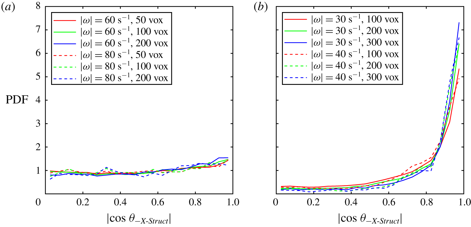
Figure 19. PDFs of the orientation of coherent vortical structures for different values of  $|\unicode[STIX]{x1D74E}|$ and structure size, for regions close to the grid (a) $x=-23$ to $-115~\text{mm}$ (P1), and near the exit of the contraction (b) $x=103$ to 198 mm (P3). Grid-rotation mode is S1. PDF calculated with 20 bins. The 100 voxel size corresponds to ${\approx}24~\text{mm}^{3}$.

Figure 20. Streamwise evolution of the PDF of orientation of coherent vortical structures versus downstream location regions P1–P3 for modes (a) S1, and (b) R. Structures are identified using the criteria: size of 100 voxels,  $|\unicode[STIX]{x1D74E}|=70~\text{s}^{-1}$ for P1; $|\unicode[STIX]{x1D74E}|=35~\text{s}^{-1}$ for P2 and P3. PDFs are plotted with 50 bins.

Figure 21. Streamwise evolution of the vertical orientation PDF of coherent vortical structures in sub-regions R1–R10, for grid-oscillation modes (a) S1, and (b) R. Structures are identified using criteria: size of 100 voxels,  $|\unicode[STIX]{x1D74E}|=70~\text{s}^{-1}$ for P1; $|\unicode[STIX]{x1D74E}|=35~\text{s}^{-1}$ for P2 and P3. PDFs are plotted with 50 bins. The mid- $x$ locations (in mm) for these sub-regions are: $-100$ (R1), $-69$ (R2), $-38$ (R3), 46 (R4), 77 (R5), 108 (R6), 120 (R7), 151 (R8), 182 (R9).
3.8 Orientation of coherent vortical structures
The analysis of vorticity orientation is now extended to large-scale coherent vortical structures. The coherent structures are identified based on the vorticity magnitude and their size. The structure identification and tagging is done using the 3-D watershed function in MATLAB. Voxels with  $|\unicode[STIX]{x1D74E}|$ higher than a particular cutoff value are flagged. A ‘turbulent structure’ here corresponds to a group of connected flagged voxels. These connected regions are then sequentially numbered using the watershed function. Numbered structures are then filtered based on their size in voxels. A large cutoff value results in relatively smaller structures, corresponding to regions close to the vortex core. Only big structures with sizes greater than a particular value are considered for the statistics. Using the regionprops3 function in MATLAB, we extract the principal axis lengths and directions of an equivalent ellipsoid, which has the same normalized central moments as the structure. Filtered structures identified at a representative time instant in measurement regions P1, P2 and P3 are shown in figure 18. The $x$–
$x$– $y$ projections show the orientation becoming more aligned with $x$ as we move through the contraction from P1 to P3, with most of the structures in P3 nearly aligned with $x$. In figure 19 we present the PDFs of the $\cos (\unicode[STIX]{x1D703}_{-X\text{-}Struct})$, where $\unicode[STIX]{x1D703}_{-X\text{-}Struct}$ is the angle between the major axis direction of the coherent structure and the $-x$-axis. The PDF of absolute value of $\cos (\unicode[STIX]{x1D703}_{-X\text{-}Struct})$ is shown as we consider only the orientation of the principal axis.
We note that the structure shape and quantity depend on the chosen vorticity magnitude and size criterion and are therefore quite subjective. Thus we quantify the sensitivity of the results on the specific choice of these thresholds. Based on the visualization of isosurfaces of  $|\unicode[STIX]{x1D74E}|$, we see that the coherent structures are distinct and clear for $|\unicode[STIX]{x1D74E}|$ in the range $60{-}80~\text{s}^{-1}$ inside P1, and $30{-}40~\text{s}^{-1}$ inside P2 and P3. The PDFs of $|\!\cos (\unicode[STIX]{x1D703}_{-X\text{-}Struct})|$, obtained for P1 and P3 for different size criteria in the above ranges of $|\unicode[STIX]{x1D74E}|$, are shown in figure 19. The maximum size in this study is chosen to ensure that large structures are identified at all the time realizations. Sizes of 50, 100, 200 and 300 voxels correspond to ${\approx}12$, 24, 48 and $72~\text{mm}^{3}$. Figure 19 shows that the cutoff values chosen have a minimal effect on the PDFs. In P1 (figure 19(a)), the alignment distribution is random. In P3 (figure 19(b)), the PDF shows strong preference towards cos $\unicode[STIX]{x1D703}_{-X\text{-}Struct}=1$ for both values of $|\unicode[STIX]{x1D74E}|$ and especially for the largest structures. This indicates that larger structures tend to align more as compared to the smaller ones. Thus for all the further analysis of structures, we use a cutoff value of $|\unicode[STIX]{x1D74E}|=70~\text{s}^{-1}$ for P1, $|\unicode[STIX]{x1D74E}|=35~\text{s}^{-1}$ for P2 and P3. In all cases only structures of size greater than 100 voxels ( ${\approx}24~\text{mm}^{3}$) are considered. For each realization, the PDF is computed using structures that satisfy the above criteria, over all of the 5499 frames. In each measurement region, the average of the PDFs over all realization is presented in figure 20(a) (average is over three realizations in P1, and four in P2 and P3). With the chosen cutoff values, we have the average of approximately 100 000 big structures in each measurement volume. It is clear that there is a strong tendency of structures to align with $x$ near the exit of the contraction in P3, with almost a random distribution at the inlet in P1. The random mode, which has a totally different grid-oscillation protocol compared to the rest, exhibits an identical trend in the PDFs (figure 20(b)). This confirms the structures tend to align in $x$-direction in a contraction irrespective of the protocol of the grid.
The evolution of the orientation along the contraction is looked at more closely by dividing each measurement region into three equal sub-regions, P1 to R1–R3, P2 to R4–R6 and P3 to R7–R9 (R1 is closest to the grid and R9 is the last one at the outlet of the contraction). The PDF of the structure orientation in each of these sub-regions for modes S1 (figure 21(a)) and R (figure 21(b)) shows a clear systematic transition from a random orientation at R1 to a preference for alignment in the vertical at the outlet of the contraction at R8. Due to the overlap of P2 and P3, sub-regions R6 and R7 also overlap and thus show nearly identical PDFs. However, in region R9, which is in the straight section downstream the contraction, the PDF shows a slightly reduced peak tendency to align with  $x$. This deorientation immediately downstream of the contraction could be physical but we will require measurements further downstream to confirm this behaviour and investigate the underlying reasons, such as the return to isotropy. This reduction in the peak PDF value persists after we increase the distance after the grid to the entrance of the contraction, as shown in the supplementary figure S12 and discussed in supplementary material § S6.
3.9 Increasing the distance between the grid and contraction
There is a trade-off between large  $Re_{\unicode[STIX]{x1D706}}$ and transverse homogeneity of the inlet flow, which requires a long distance between the active grid and the entrance of the contraction. To address whether this inhomogeneity has significant effect on the vortical-orientation results, we have performed an additional experiment where this distance was doubled from $x/M=8$ to 16, as shown in figure 2(a). Thormann & Meneveau (Reference Thormann and Meneveau2014) conclude that the traverse spatial homogeneity was found to be good beyond $x/M\approx 15$ in their study on decay of turbulence behind active fractal grids. This was done for the primary synchronous mode S1, which showed the large inhomogeneity in figures 7(b) and S9(a). While the value of $Re_{\unicode[STIX]{x1D706}}$ is more than cut in half, the orientation results are essentially the same, as will now be shown. The bottom part of table 1 lists the conditions at the inlet of the contraction with the additional length. Figure 22(a) presents the inlet inhomogeneity of the mean flow, showing that the maximum has reduced from $\pm 6\,\%$ in figure 7(b), to $\pm 3\,\%$. Figure 22(b) shows the orientation of the vorticity vector with respect to the principal rates of strain. Compared to figure 13(c) the results are quite similar. Similarly, figure 22(c) shows that the orientation of the pointwise vorticity vector with the vertical centreline is the same as in figure 15. Finally, figure 22(d) also shows that the orientation of the large-scale coherent structures is essentially the same as in figure 20(a). Here the vorticity level of the isocontour must be adjusted to a smaller value to account for the diffusion of vorticity further downstream from the grid.

Figure 22. Results obtained from experiments for which the length of the straight section between the active grid and the inlet of the contraction is doubled from  $x/M=8$ to 16. All results presented are for mode S1. (a) Transverse profiles of $\langle U\rangle (y)$ normalized by $\langle U_{lm}\rangle$ at different $x$-locations are presented in comparison to figure 7(b). The profiles marked by dotted lines are obtained from experiments with the extension added. (b) PDF of cosine of the angle between $\unicode[STIX]{x1D74E}$ and the principal strain-rate eigenvectors at $x=142~\text{mm}$, as compared to those in figure 13(c). (c) The alignment PDF of $\unicode[STIX]{x1D74E}$ with respect to the tunnel centreline at different $x$-locations, as compared to figure 15. (d) Streamwise evolution of PDF of the orientation of coherent vortical structures in regions $\text{P}2^{\ast }$ ( $x=3{-}109~\text{mm}$) and $\text{P}3^{\ast }$ ( $x=86{-}192~\text{mm}$). Here, $\text{P}2^{\ast }$ starts 20 mm above the previous region P2 and is closer to the inlet of contraction. Structures are identified using the two criteria of size ${>}100$ voxels and $|\unicode[STIX]{x1D74E}|=20~\text{s}^{-1}$ (refer to figure 20(a) for comparison). PDFs are evaluated with 50 bins.
3.10 Experiment at larger optical magnification
Our experiments are focused on capturing the larger-scale coherent vortices in the turbulence and cannot resolve all the small scales and the velocity gradients accurately. Thus, in order to evaluate the effect of the spatial resolution, we repeat an experiment using a higher optical zoom ( ${\sim}2\times$). The measurements were made in a region $30\times 50~\text{mm}$ approximately centred on the location of the maximum contraction curvature. We use these data to assess the accuracy of the vorticity and the dissipation rate, as described in the supplementary material § S7. The PDF of the vorticity magnitudes is slightly shifted to higher values, as shown in supplementary figure S15. Similarly, the dissipation shows values up to 2.8 times higher than for the less zoomed imaging. However, this results in only 25 % smaller estimates of the Kolmogorov scale due to its weak dependence on $\unicode[STIX]{x1D700}^{-1/4}$.
4 Discussion and conclusions
Herein we have attempted to determine the evolution of turbulent vortical structures as they convect through a two-dimensional contraction. We have used the latest tomo-PIV and STB algorithms to measure the time-resolved velocity field in volumetric slices upstream of and within the contraction.
We have used active oscillating grids to increase the energy of the turbulent fluctuations. We have also kept the entrance of the contraction quite close to these grids to retain the large  $Re_{\unicode[STIX]{x1D706}}\approx 250$. The trade-off is here between the vigour of the turbulence and the transverse homogeneity of the mean and turbulent quantities. We believe the transverse inhomogeneities are sufficiently small not to affect the dynamics of the coherent vortices as they are accelerated and strained by the converging stream. This is indeed verified in an additional experiment (§ 3.9), where the distance from grid to contraction is doubled, to $x_{AG}/M=16$. The principal vortical-alignment results were unaffected.
The random grid-oscillation mode shows the largest turbulence intensity, but we see similar statistical trends for all of the five grid-oscillation modes, even for the pathological ones with all grids rotating in the same direction. The streamwise  $u_{rms}$ reduces monotonically through the entire contraction, consistent with the linear theory and earlier hot-wire measurements for small contraction ratios. The cross-stream velocity component r.m.s. values increase modestly. The fluctuations $w_{rms}$, as well as $\unicode[STIX]{x1D714}_{x,rms}$ and $\unicode[STIX]{x1D714}_{y,rms}$, show small local maxima at the maximum local curvature of contraction, which occurs somewhat downstream of the peak axial strain-rate location.
While we cannot fully resolve the finest scales of the flow and pointwise statistics could be better resolved with hot-wires or large-magnification planar PIV, we highlight that the strength of our experimental method is the volumetric large-scale measurements. We exploit this to visualize and track coherent vortical structures using isosurfaces of constant  $|\unicode[STIX]{x1D74E}|$, along with a minimum size criterion. Conditional averaging shows that, immediately downstream of the active grid and before the contraction, the coherent vortical structures have arbitrary orientation. They then get stretched by the mean strain along the contraction, resulting in elongated structures strongly oriented with the centreline $x$-axis at the contraction exit. The orientation of these structures is determined by the major principal axis corresponding to the equivalent ellipsoids. This is evaluated by PDFs of the cosine of the angle between these ellipsoids, or $\unicode[STIX]{x1D74E}$ and the vertical $x$-axis at different streamwise locations. The PDFs in figures 20 and 21 show clearly the systematically increasing alignment through the contraction.
To quantify the strength of this alignment with the mean strain, we can look at the ratio of the probability peak in figures 19–21, where the two are nearly perfectly aligned, compared with the value in the low-probability plateau, i.e.  $p(\unicode[STIX]{x1D703}=\unicode[STIX]{x03C0}/2)/p(\unicode[STIX]{x1D703}\simeq 0)$. For the pointwise vorticity vector in figure 15 this ratio is ${\sim}4$ near the exit of the contraction, while for the large-scale coherent vortical structures this ratio becomes as large as ${\sim}30$ in figure 21. For comparison, by this measure of the alignment, the alignment of vorticity and large-scale strain is weaker for homogeneous turbulence, showing only a ratio of ${\sim}5$ in Hamlington et al. (Reference Hamlington, Schumacher and Dahm2008). However, the straining of the turbulent large scales is certainly not as persistent as in our imposed external configuration.
We have quantified the degree of preferred alignment of  $\unicode[STIX]{x1D74E}$ with the intermediate eigenvector of the strain-rate tensor as well as with the large-scale strain for our turbulent flow subject to the contraction. These findings are of relevance, in the context of LES to the development of subgrid-scale (SGS) stress tensor models, especially those which are structure based (Lesieur et al. Reference Lesieur, Métais and Comte2005). One such SGS model is the stretched spiral vortex model originally developed by Misra & Pullin (Reference Misra and Pullin1997). In their work they consider that, embedded within each computational cell, there exists a superposition of stretched vortices, each having orientation taken from a probability density function. They proposed a two-vortex model in which a fraction of the local subgrid structures tend to become aligned with the extensional eigenvector and the remainder align with the intermediate eigenvector. Later works by Cheng, Pullin & Samtaney (Reference Cheng, Pullin and Samtaney2015, Reference Cheng, Pullin and Samtaney2018) and Cheng et al. (Reference Cheng, Pullin, Samtaney, Zhang and Gao2017) orient the subgrid vortex along the extensional eigenvector. In our experiments, one may consider the large-scale strain imposed by the contraction as an analogue to the background strain experienced by the subgrid vortex in the stretched spiral vortex SGS model. Hence, the alignment of the vortical structures after the contraction in our experiments is in a sense a validation of the assumption of orientation along extensional eigenvectors in the stretched spiral vortex SGS model. Our experimental results may serve as a guide to other models that rely on a vortex structure approach in LES modelling.
This work suggests numerous extensions. It remains, for example, to investigate whether individual coherent vortical structures persist through the entire contraction, which would require employing multiple tomo-PIV systems along the streamwise direction.
Acknowledgements
This study was supported by King Abdullah University of Science and Technology (KAUST) under grant URF/1/2981-01-01. We thank S. Taguchi and Y. Otsu for their help in running some of the early experiments. We acknowledge the help of R. Carolan for designing the active grids and M. Abdulkareem for programming them.
Supplementary material
Supplementary material is available at https://doi.org/10.1017/jfm.2019.887.


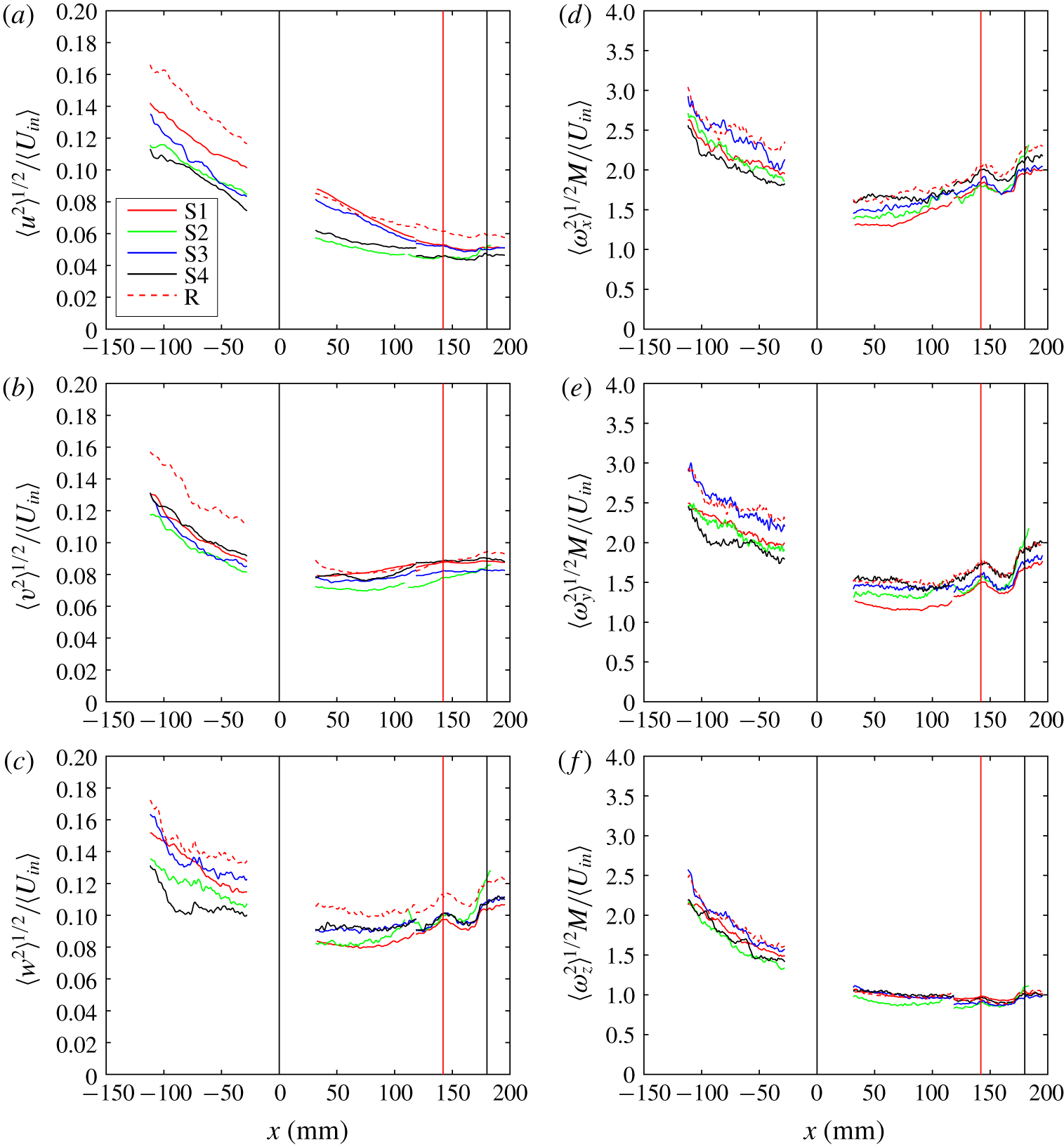


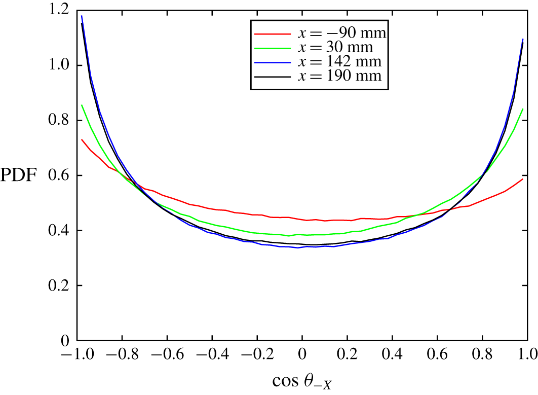


 Open access