


1. Introduction
In the first decade of the 21st century the majority of tidewater outlet glaciers of the Greenland ice sheet steadily retreated at a rate in excess of 100 m a–1, on average (Reference Moon and JoughinMoon and Joughin, 2008). In most cases, this pattern of retreat has coincided with a trend of increasing surface speeds (Reference Moon, Joughin, Smith and HowatMoon and others, 2012). In addition, higher rates of frontal ablation (the sum of calving and submarine melt) have resulted in rapid thinning on many of Greenland’s largest outlet glaciers (Reference Thomas, Frederick, Krabill, Manizade and MartinThomas and others, 2009). As mass losses at the calving fronts of outlet glaciers make up a large fraction of observed mass loss of the Greenland ice sheet (Reference Rignot and KanagaratnamRignot and Kanagaratnam, 2006; Reference Pritchard, Arthern, Vaughan and EdwardsPritchard and others, 2009; Reference Van den BroekeVan den Broeke and others, 2009), such widespread changes on outlet glaciers have the potential to increase rates of mass wastage and its contribution to global sea level.
There is a growing body of evidence showing that the rapid changes seen at Greenland outlet glaciers are primarily driven by changes at the glacier front (Reference JoughinJoughin and others, 2008; Reference Nick, Vieli, Howat and JoughinNick and others, 2009, Reference Nick2013). The forcing that drives these changes at the glacier termini seems to be, at least partially, related to climate, through warmer ocean waters along the coast of Greenland (Reference Holland, Thomas, De Young, Ribergaard and LyberthHolland and others, 2008; Reference Howat, Joughin, Fahnestock, Smith and ScambosHowat and others, 2008; Reference Motyka, Truffer, Fahnestock, Mortensen, Rysgaard and HowatMotyka and others, 2011). Changes initiated at the terminus are then propagated inland as changes in ice thickness and surface slope (Reference JoughinJoughin and others, 2012). Such rapid, dynamic changes in geometry have allowed the Greenland ice sheet to respond to climate perturbations at a rate much faster than predicted by the response to surface mass-balance forcing alone (Reference NyeNye, 1960).
Constraining the response of outlet glaciers to climate forcing on decadal timescales demands a solid understanding of dynamic processes occurring over short time-scales. These include perturbations to glacier motion from iceberg calving, ocean tides and surface meltwater forcing, with the potential for altering outlet glacier geometries. While changes in the length and thickness of outlet glaciers are most pronounced near glacier termini, carrying out in situ measurements in the near-terminus region of tidewater glaciers is notoriously challenging, due to rapid flow speeds, heavy surface crevassing and iceberg calving. While remote-sensing methods have improved a great deal, repeat cycles of a week or more limit investigations of glacier processes on short timescales.
Outlet glacier response to large-scale calving events and, where applicable, ice-shelf retreat has been documented in Greenland (Reference Luckman and MurrayLuckman and Murray, 2005; Reference NickNick and others, 2012) and Antarctica (Reference Scambos, Bohlander, Shuman and SkvarcaScambos and others, 2004). These results demonstrate a pattern of glacier acceleration and thinning following the catastrophic collapse of ice shelves or floating tongues, consistent with ice-shelf buttressing hypotheses (Reference Dupont and AlleyDupont and Alley, 2005). While reduced in magnitude and reach, the response to smaller calving events, that do not involve the collapse of an entire floating tongue, is of a similar nature, displaying increases in speed and extension and/or thinning (Reference Amundson, Truffer, Lüthi, Fahnestock, West and MotykaAmundson and others, 2008; Reference NettlesNettles and others, 2008; Reference Rosenau, Schwalbe, Maas, Baessler and DietrichRosenau and others, 2013). A predictable response to calving events over a continuum of magnitudes illustrates that, while response to smaller calving events is limited in spatial and temporal scope compared with catastrophic retreats, such events play an important role in outlet glacier dynamics by controlling glacier geometry near the terminus.
The forcing imposed by unpredic glacier calving activity has proven to be a challenging problem to model, but the periodic forcing applied to tidewater glaciers by ocean tides is easily predicted. However, the wide range of glacier responses to the consistent forcing provided by tides demonstrates the diversity of tidewater glacier systems. In Antarctica, evidence of ice-stream response to tidal forcing has been observed as far as 80 km inland of the grounding zone (Reference Anandakrishnan, Voigt, Alley and KingAnandakrishnan and others, 2003), while results from Alaskan tidewater glaciers indicate a far less extensive response of a few kilometers or less (Reference WaltersWalters, 1989; Reference O’Neel, Echelmeyer and MotykaO’Neel and others, 2001). In Greenland, the behavior in response to tidal forcing falls between Antarctic and Alaskan end members; results from Helheim Glacier (De Reference De JuanJuan and others, 2010) show tidal response extending up to ~ 10 km from the terminus.
Despite the emphasis on variations, the flow of tidewater glaciers tends to be more steady than that of other glacier systems (Reference ClarkeClarke, 1987). This has been particularly true of Greenland’s fastest tidewater outlet, Jakobshavn Isbræ, where speeds have been very steady over intra-annual timescales (Reference Echelmeyer and HarrisonEchelmeyer and Harrison, 1990; Reference Luckman and MurrayLuckman and Murray, 2005; Reference Podrasky, Truffer, Fahnestock, Amundson, Cassotto and JoughinPodrasky and others, 2012). Velocity variations occurring on sub-seasonal timescales are obscured by the exceptionally high flow speeds, as much as 12 km a–1 (Reference JoughinJoughin and others, 2012), along the main channel of the glacier. However, since the break-up of the floating tongue in the early 2000s, with the ensuing terminus retreat of >12 km (Reference Podlech and WeidickPodlech and Weidick, 2004) and doubling of speed (Reference Joughin, Abdalati and FahnestockJoughin and others, 2004), Jakobshavn Isbræ has progressively retreated and sped up from year to year. Along with higher yearly average flow speeds, the drastic change in terminus geometry of Jakobshavn Isbræ has increased glacier sensitivity to ice-flow perturbations coming from seasonal variations in terminus position (Reference JoughinJoughin and others, 2008; Reference Joughin and SmithJoughin and Smith, 2013), calving (Reference Amundson, Truffer, Lüthi, Fahnestock, West and MotykaAmundson and others, 2008) and surface meltwater forcing (Reference Podrasky, Truffer, Fahnestock, Amundson, Cassotto and JoughinPodrasky and others, 2012).
This study aims to identify and quantify short-term flow variations at Jakobshavn Isbræ by decomposing time series of glacier motion with a suite of simple models to identify the relative influence of the sources responsible for forcing short-term variations. We examine 14 days of high-time-resolution motion data recorded in the near-terminus region of Jakobshavn Isbræ during August 2009. A 14 day observation period was chosen because previous experience indicated that at least one large calving event should occur during that period (Reference Amundson, Clinton, Fahnestock, Truffer, Lüthi and MotykaAmundson and others, 2012). Two simple models for explaining glacier response to ocean tidal forcing and a single, large iceberg-calving event are used to estimate the strength of variations attributable to these two modes of forcing at the terminus. Once quantified, the responses to a single large calving event and periodic tidal forcing are then compared with background motion, described by a simple linear model.
2. Data and Methods
2.1. GPS and theodolite data
We occupied three temporary GPS sites during a 12 day period in August 2009 (Fig. 1) with dual-frequency receivers that recorded with a 15 s sampling interval. GPS data were processed kinematically with Track (v. 1.22), part of the GAMIT/GLOBK GPS processing package (Reference ChenChen, 1999) with typical baseline distances of 5–50 km. In addition, we placed five optical markers at sites 1–2 km from the terminus (Fig. 1). The optical targets were surveyed with a Leica 1610 automatic theodolite and a DI3000S distomat. Two additional reference targets were placed on bedrock in the forefield to correct for small amounts of motion due to thermal expansion of the steel theodolite stand. The known distances to the reference targets combined with measurements of ambient air temperatures were used to correct for refractive errors in distance measurements to the optical targets located on the glacier. Measurements of optical marker positions were repeated approximately every 10–15 min during the 14 day study period (Fig. 2). However, the record of theodolite positions was interrupted during certain time periods due to windy conditions. Horizontal position data of each site were rotated into a local flow-parallel direction.
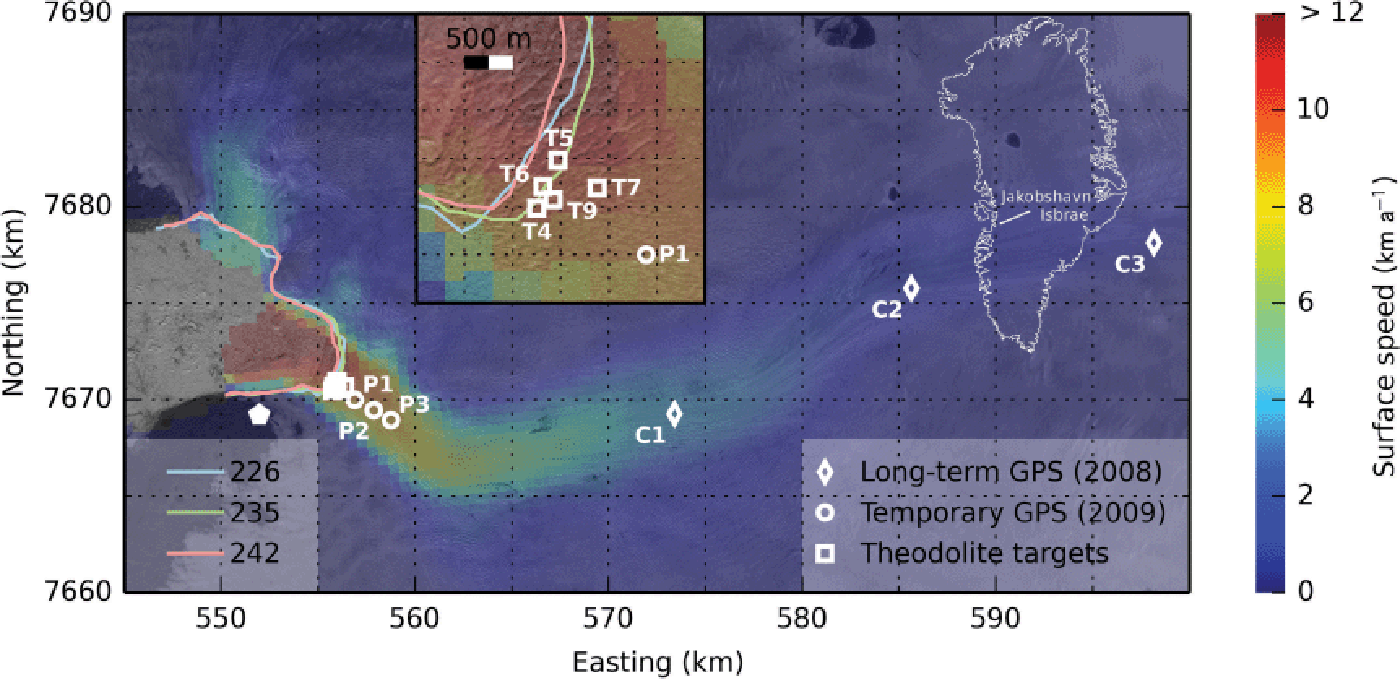
Fig. 1. Day 218, 2009 SPOT (Satellite Pour l’Observation de la Terre) scene showing the Jakobshavn Isbræ study area. The image is overlaid with surface speeds from a 2008 synthetic aperture radar mosaic of Greenland (Reference Joughin, Smith, Howat, Scambos and MoonJoughin and others, 2010). White symbols mark the locations of long-term GPS (2008 data), temporary GPS and theodolite optical targets. The location of the GPS base station and automatic theodolite is marked by the white pentagon. The inset shows the near-terminus region at a magnification of 5:1. Terminus outlines digitized from Landsat 7 scenes acquired on days 226, 235 and 242 are shown in blue, green and red.
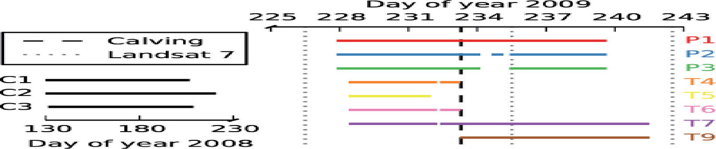
Fig. 2. Coverage of GPS and theodolite data for the 2009 and 2008 datasets. C1, C2, C3, P1, P2, etc. are the GPS stations. The color coding for the 2009 stations is continued through the following figures. The dashed line marks the timing of the calving event on day 233, and dotted lines indicate the timing of Landsat 7 scenes used to digitize the ice front.
Due to large baseline distances, the theodolite data are subject to large errors relative to the GPS measurements. Some of these errors are obvious outliers, far removed from the rest of the data. More often, theodolite errors are smaller and can be attributed to instrumental error and atmospheric delays. The theodolite data were detrended with a best-fit linear model, and data points more than one standard deviation away from the trend were identified as outliers and excluded from the analysis. Once outliers were removed, the position data were smoothed to reduce the influence of measurement error. A local quadratic regression filter (LOWESS), implemented with MATLAB® (v. 7.14), was used for smoothing the theodolite data with a smoothing window of eight data points, or ~ 2 hours. Position data from GPS were down-sampled, using an interval-averaging routine, to an interval of 15 min. Position time series of GPS sites were not smoothed after resampling. We include results of GPS data in 2008 from a previous study (Reference Podrasky, Truffer, Fahnestock, Amundson, Cassotto and JoughinPodrasky and others, 2012), to provide estimates of surface speed and constrain the response to ocean tides at positions 20–50 km upstream of the terminus. However, as these data are from the previous year, we do not include them in the calving- and tidal-response analyses of this study.
2.2. Iceberg calving
During the study period, a large calving event occurred on day 233; this was the only calving activity during the 14 day period. The precise timing of calving onset was constrained with passive seismic data (Reference Amundson, Clinton, Fahnestock, Truffer, Lüthi and MotykaAmundson and others, 2012) acquired near the GPS base station. This is the same calving event as that discussed by Walter and others (2012) and it triggered a global seismic response (Reference Veitch and NettlesVeitch and Nettles, 2012). It is difficult to accurately determine terminus changes from oblique photographs, because sea level at the calving front was generally obscured by large icebergs and the height of the terminal cliff is not well known. However, the magnitude of the calving event can be qualified with time-lapse photography near the terminus, and tide data measured in the inner fjord. We can constrain the change in terminus position due to calving and glacier motion using satellite remote-sensing data. Terminus positions were determined for three days in August with available Landsat scenes. The calving front was digitized from scenes on days 226, 235 and 242. The distance from each site to the terminus was estimated by integrating the length of a flowline from each site to the terminus. Flowlines passing through GPS and theodolite markers were calculated using 2008 synthetic aperture radar velocity data (Reference Joughin, Smith, Howat, Scambos and MoonJoughin and others, 2010).
Reference Amundson, Truffer, Lüthi, Fahnestock, West and MotykaAmundson and others (2008) described response to calving as a step-change in glacier speed. We modeled the horizontal position response to calving, ξ calv, with a piecewise, second-order polynomial

with two intervals and an interior knot, t c, at the time of the calving event on day 233. The best-fitting kinematic parameters, a, v and ξ 0, were determined using a linear least-squares optimization. To ensure continuity of modeled positions for both time intervals, ξ 0 was constrained to the same value before and after the calving event. We applied the calving model to six days of position data centered about t c.
As a consequence of extraordinarily large longitudinal strain rates in the terminus region of Jakobshavn Isbræ, the second-order terms, a 1 and a 2, encompass the effects of motion through a velocity gradient as well as Eulerian acceleration. It is necessary to separate the combined effects in order to estimate values of pre- and post-calving acceleration at the GPS and optical markers. Here we used methods similar to those described by Reference Amundson, Truffer, Lüthi, Fahnestock, West and MotykaAmundson and others (2008) and Reference Podrasky, Truffer, Fahnestock, Amundson, Cassotto and JoughinPodrasky and others (2012). Podrasky and others’ Eqn (4) reads
where ξexp is the horizont0061l position and u 0 is the along-flow velocity at initial time, t 0. The combined acceleration term,
is the sum of longitudinal strain rate, ![]() ξ,0, and a constant, relative acceleration term, where the acceleration is assumed to be proportional to velocity, u. Expanding Eqn (2) gives
ξ,0, and a constant, relative acceleration term, where the acceleration is assumed to be proportional to velocity, u. Expanding Eqn (2) gives
which has the same form as Eqn (1). Equating with ξcalv With ξexp implies ν =u0 and
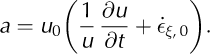
Over small time intervals, u ≈ u 0 and
Using strain rates estimated from GPS and theodolite data, along with parameters a and v, we used Eqn (6) to solve for the Eulerian accelerations, ∂u= ∂t, in the days before and after large calving events.
2.3. Tidal analysis
Tides were measured with a pressure transducer in the ice fjord within 5 km of the calving front concurrent with the 14 days of ice motion measurements. A longer record from Ilulissat shows close agreement with tides in the ice fjord. The Ilulissat tide record was analyzed with the T_TIDE package (Reference Pawlowicz, Beardsley and LentzPawlowicz and others, 2002) in order to identify the strongest tidal constituents.
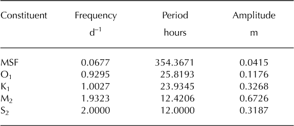
The amplitude, frequency and names of significant tidal constituents are listed in Table 1. The tides measured in the inner fjord incorporate noise, including surface waves generated by calving events and other sources, as well as a small instrumental error. While the measured tides provide valuable information, such as the timing of major calving events, the record of tidal stage in the inner fjord does not fully cover the time span of glacier motion data. We used the longer record of tides recorded at Ilulissat to analyze the tidal response of the glacier. The two tidal datasets are in close agreement, with no measurable delay in time and maximum difference in stage <10 cm. While the Ilulissat record has much less noise than the fjord measurements, some sources of noise are still present. Sources of noise include instrumental error and waves generated by major calving events in the inner fjord. To eliminate the noise in the Ilulissat tide data, we solved for the amplitude, A, and phase, ϕ, of known frequencies, f, of the major tidal constituents identified using T_TIDE. The smooth, noiseless ocean tide model,
Table 1. Strongest constituents of the tidal record in Ilulissat Icefjord
was used in subsequent steps of the tidal analysis.
We calculated daily values of tidal admittance, Λ, defined as the ratio between tidal response and tidal height, H. Tidal response was evaluated for horizontal (along-flow) and vertical components of glacier motion at each site and for each day of data. Day-long records of position data were first detrended to remove the background signal associated with rapid, constant-speed motion. The method we employed for calculating tidal admittance uses position data, not speeds. By using position data directly, the calculations are subject to less noise than would be introduced by differentiating to produce velocity time series. However, assuming ocean tides modulate ice flow, the tidal response will be expressed in the slope of glacier-position time series and it is not possible to directly compare horizontal glacier positions with tidal height.
To determine the influence of tides on glacier motion we propose a simple model based on reconstructed tides to explain the variability of detrended positions. Tide data were modified using two parameters to best-fit position data: phase difference between tides and detrended position, and an amplitude multiplier (admittance). A grid search method was used to find the optimal parameters (phase and admittance) for modeling tidal response each day.
Three plausible hypotheses (or a combination thereof) can explain the relation of horizontal motion to tides. (1) Tides may modulate glacier flow through an elastic response to changing pressure on the vertical calving face, in which case glacier position and tides will be anti-correlated. (2) Ocean tides could affect basal water pressure in the terminus region, thereby influencing basal motion, and surface speeds will be correlated with tidal height. (3) The glacier may respond viscously to perturbations in horizontal compressive stress exerted by tides, resulting in variations of along-flow strain rate, and surface speed will be anticorrelated with tidal height. Additionally, tidal height and glacier position will experience a phase difference of 90º, due to a phase shift between position and speed. To allow for these possible modes of tidal response, we searched over both positive and negative values of tidal admittance. However, when modeling vertical admittance we only optimized for positive values of tidal admittance. We searched over a 1001 × 41 grid of tidal admittance, Λm (in steps of 0.0005), and time delay, δtn (in steps of 10 min), to find the best-fitting model for tidal response that minimizes the X2 difference between measured, detrended positions, ξlin, and modeled positions, while accounting for position uncertainty, σξ:
We used two criteria for evaluating the physical and statistical validity of each day’s model results. Results for horizontal tidal admittance with positive phase differences between modeled positions and tides were excluded, on the basis that the response to tides cannot precede the tidal forcing. F –tests (Reference Lomax and Hahs-VaughnLomax and Hahs-Vaughn, 2007) were performed on the results for each day to validate the significance of the model. Results without a statistically significant model were excluded from further analysis.
Tidal analysis of the 2008 GPS data at sites C1–C3 was performed using a different method, because no measurements of tides were available during that period. To calculate admittances at these sites, we took the ratio of the amplitude at the M2 frequency (semidiurnal lunar), from analysis of position data using T_TIDE, and the amplitude of the M2 ocean tide constituent in Table 1. This method is similar to the approach used by Reference O’Neel, Echelmeyer and MotykaO’Neel and others (2001), and assumes that the only source of modulation at the M2 frequency is due to ocean tides and that the response to tidal forcing is uniform across all tidal constituents.
3. Results
3.1. Ice motion
Processing the GPS observations resulted in position time series for the three P-sites spanning days 228–239 (in 2009). Power failures resulted in limited periods of missing data at sites P2 and P3. At the temporary GPS sites, we estimated a 10 mm uncertainty in horizontal positions and a 20 mm uncertainty in vertical positions, by examining the level of noise present in brief spans of data. GPS observations at the long-deployment C-sites were processed over a longer time span during 2008, a year prior to the measurements acquired for the current study. At these continuous sites, we estimated a 6 mm uncertainty in horizontal positions and 20 mm in vertical positions, based on the level of noise apparent in short segments of position time series. Theodolite-measured horizontal positions have an estimated uncertainty of 70 mm; for vertical positions we estimated an uncertainty of 100 mm. Some of the optical targets were placed very near the terminus, and during the large calving event on day 233 three of the targets were destroyed. One optical target that was not visible at the time of deployment, could be measured following the calving event.
Time series of vertical position at the GPS sites vary steadily with time, while vertical positions of the optical markers display a greater degree of variability (Fig. 3). Curiously, the vertical time series for site P1 shows steadily increasing vertical position over the study period. The total upward motion at P1 was ~3 m over a period of 12 days. This upward vertical trajectory was only observed at P1.
Fig. 3. Vertical trajectories of the three temporary GPS markers (P1, P2 and P3) and optical marker T7. The lowest GPS site, P1 (red), experienced steady upward motion totaling 3 m over 12 days.
Ice surface speeds were highest near the calving front and rapidly decayed with distance upstream. A maximum speed of 48 m d–1 was recorded after the calving event on day 233 at an optical target located ~1 km from the front. Surface speeds decreased to ~10 m d–1 at a distance of 20 km and decreased more gradually at greater distances (Fig. 4). Our surface speeds agree well with observations of Reference JoughinJoughin and others (2012).

Fig. 4. Daily-average surface speeds at GPS (circles) and optical marker (squares) locations, used to detrend each day’s position data prior to performing the tidal analysis. Points are color-coded by day of year. Black diamond markers indicate mean speeds from the 2008 dataset for reference. The gray-shaded region indicates the range of the inset figure.
The distribution of speeds over the lower glacier is consistent with the large longitudinal strain rates in the terminus region (Fig. 5). The greatest strain rates were found between the lowest pair of sites, P1 and T7, with typical values of 2–4 a–1, decreasing to ~0.25 a–1 2 km upstream.

Fig. 5. Longitudinal strain rates between one optical target and temporary GPS sites: between P1 and T7 (black), P2 and P1 (gray) and P3 and P2 (light gray). Strain rates between P1 and T7 have much more scatter due to the greater uncertainties in theodolitemeasured positions at site T7. Curves are annotated with the mean distance to the terminus. The timing of a large calving event on day 233 is marked by a vertical dashed line.
Glacier surface speeds at sites nearest the terminus experienced the greatest degree of variability. Ice surface speeds in the near-terminus region exhibited variability at diurnal and semi-diurnal frequencies. They also displayed transient velocity features and sudden changes in speed (Fig. 6). Short-term variability at long-deployment GPS sites was primarily diurnal, but also included episodic changes in speed ~10% of average speed (Reference Podrasky, Truffer, Fahnestock, Amundson, Cassotto and JoughinPodrasky and others, 2012). In all cases, the amplitude of these variations is small in proportion to the magnitude of background speeds. The magnitudes of short-term variations amount to 5–10% of background at all sites.
Fig. 6. Time series of surface speeds at optical targets and temporary GPS sites (T- and P-sites). The timing of a large calving event on day 233 is marked by a vertical dashed line.
3.2. Iceberg calving
A major calving event was documented using time-lapse photography on day 233, and the precise timing of onset, 06.56 UT, was identified in the seismographic record. This was the only major calving event recorded during the study. Full-thickness icebergs (~900 m) were evacuated as far back as 500 m from the calving front along a 2–3 km stretch of the terminus, as estimated from time-lapse photography and later satellite imagery (Fig. 1). This was typical of the large calving events that occurred every 1–2 weeks during the previous summers (Reference Amundson, Clinton, Fahnestock, Truffer, Lüthi and MotykaAmundson and others, 2012). The loss of calved ice resulted in a significant change in terminus position and shortened the distance from the ice front to the GPS and optical targets by ~500 m. The change in distance to the calving front was quantified as described in Section 2, and distance values were updated at the time of the calving event on day 233. While the calving event occurred 2 days before the position of the terminus was digitized, we assumed that distance to the terminus did not change significantly from day 233 to 235, because no other large calving event occurred during that time. We examined the error from this assumption by estimating the change in length of the lower glacier due to longitudinal strain. Applying a strain rate of 3 a–1 to the two days of motion results in a strain of ~2% or a length change of only 20 m.
Following the large calving event, the near-terminus region experienced a step-increase in speed (Table 2), as previously described (Reference Amundson, Truffer, Lüthi, Fahnestock, West and MotykaAmundson and others, 2008; Reference NettlesNettles and others, 2008). This type of response was observed at the temporary GPS locations, but was not seen at the continuous GPS sites located further upstream.
Table 2. Change in speed and Eulerian accelereration in response to iceberg calving
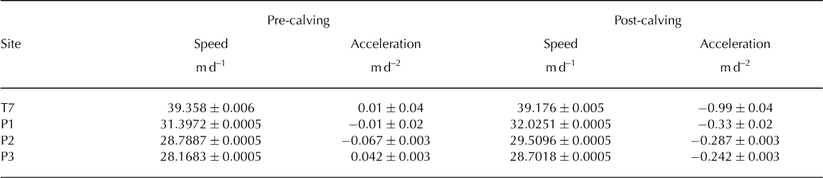
Results from the constant-acceleration model for glacier response to calving at the near-terminus sites indicate that there was little to no Eulerian acceleration, ∂u= ∂t, in the days preceding the event. However, there was a consistent pattern of deceleration in the days following calving (Table 2; Fig. 7), though glacier speeds were greater in the days after the calving event than before (Fig. 6). The calving model was only applied to sites with data both before and after the calving event (P1–P3 and T7), but the surface speeds at site T9 suggest a post-calving deceleration greater than that recorded at other sites (Fig. 6). The deceleration at T9 was estimated to be as much as 2–3 m d–2.
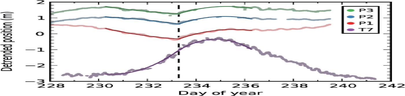
Fig. 7. Detrended position (light points) and calving-response models (solid curves) for sites P1–P3 and T7. The timing of a large calving event on day 233 is marked by a vertical dashed line.
The sharp breaks in slope of the calving models for the P-sites echo the findings of Reference Amundson, Truffer, Lüthi, Fahnestock, West and MotykaAmundson and others (2008), who identified a step-increase in speeds following a series of large calving events in 2007. However, the calving model for site T7, ~0.5 km from the terminus, transitions from decelerating to accelerating with a minimal change in speed (Fig. 7).
3.3. Tidal analysis
Horizontal and vertical tidal admittances were calculated at each site for each day of data with a statistically significant tidal-response model. Figure 8 shows the time series of daily tidal admittances for the temporary GPS sites. In the near-terminus region we found that tidal height and glacier speed were anticorrelated and higher surface speeds occurred during low tide, while speeds were lower at high tide. Because tidal height and surface speed were anticorrelated, the extrema of horizontal position were concurrent with the inflection points of tidal height, when the tide was changing most rapidly (Fig. 9). This implies a phase difference between extrema of detrended horizontal position and tidal height where maxima in detrended position lag maxima in speed by 3 hours when forced by tidal frequencies of ~2 d–1.
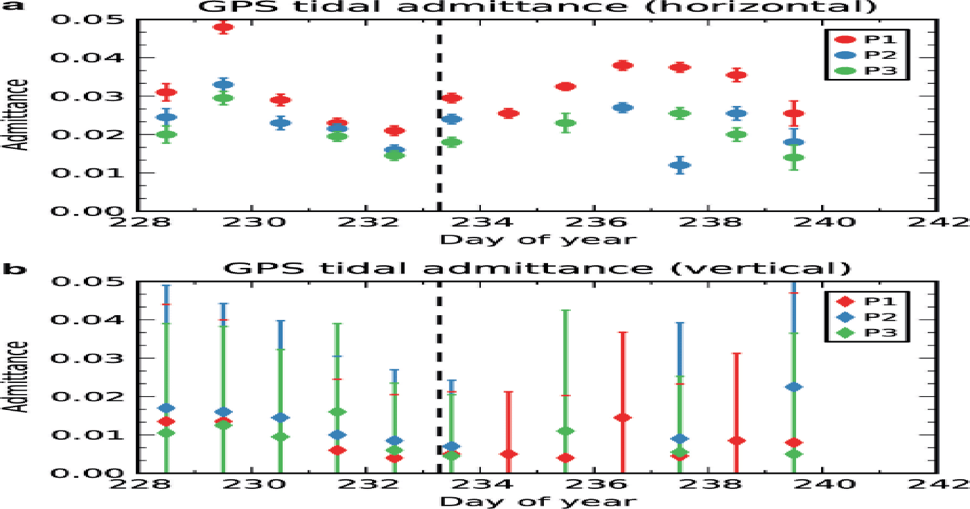
Fig. 8. Daily tidal admittance for 12 days of measurements at temporary GPS sites. The timing of a large calving event on day 233 is marked by a vertical dashed line.
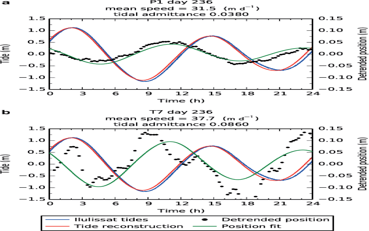
Fig. 9. Results of tidal analysis on day 236 at sites (a) P1 and (b) T7. Measured tides are shown in blue. The red curve shows the tidal model used in the analysis. Black points show measured positions, and the green curve is the best-fitting model of tidal response.
Within the limits of uncertainty, tide-induced vertical motion was in phase with ocean tides. For both horizontal and vertical admittance the degree of phase uncertainty between tides and glacier response limits our ability to identify any time delay between forcing and response or propagation times of response between measurement sites. Any such delays, if present, were shorter than ~1 hour.
Error bounds on tidal admittances at the optical markers are significantly greater than at the GPS sites. This is a result of the lower sampling rate at the optical markers, in addition to greater uncertainty of individual position measurements at these sites.
By calculating a tidal admittance for each day of position data, we were able to examine changes in tidal response as a function of time. Time series of tidal admittance at GPS sites show a trend of decreasing admittance leading up to the day 233 calving event (Fig. 8). Tidal admittance at these sites was more variable in the days following calving, but suggests a trend of increasing tidal response after the calving event.
Time series of tidal admittance at optical markers are less informative because only one marker covered the time before and after the calving event on day 233 (Fig. 2). In addition, the admittance uncertainties of optical marker data are much larger than those for the GPS data.
4. Discussion
4.1. Temporal changes in response to forcing
We have attempted to describe surface speeds in the near-terminus region of Jakobshavn Isbræ by decomposing horizontal position time series with three models: a linear fit to positions, a calving-response model and a tidal-response model.
Linear model
By far the dominant signal over the 2 week study period is explained by the first model. At all study sites, >99.9% of the variance in positions can be accounted for by a linear fit to position data. This implies that, while on interannual timescales the surface speed of Jakobshavn Isbræ has more than doubled since the late 1990s (Reference Joughin, Abdalati and FahnestockJoughin and others, 2004; Reference Joughin and SmithJoughin and Smith, 2013), variations over shorter timescales are much smaller.
Calving-response model
The greatest deviations from the linear model are explained by the calving-response model. The calving-response model assumes simple, constant-acceleration motion for two 3 day periods before and after the calving event on day 233. This model explains 93.8–99.4% of the variance remaining after detrending the motion data with the linear model. Results from the calving model show that the glacier responded to the calving event with a step-change in speed, as previously described by Reference Amundson, Truffer, Lüthi, Fahnestock, West and MotykaAmundson and others (2008) and Nettles and others (2008). Additionally, we observed a transient deceleration following calving, similar to results on Jakobshavn Isbræ from 2010 reported by Reference Rosenau, Schwalbe, Maas, Baessler and DietrichRosenau and others (2013) using photogrammetric techniques.
The ice-flow response to calving seen at Jakobshavn Isbræ could be explained by a number of mechanisms. First, the nature of iceberg calving observed at Jakobshavn Isbræ results in a sudden, large loss of ice and a rearrangement of the glacier geometry in the near-terminus region. Following such calving events, the fresh ice front has a greater vertical freeboard and the stress state is altered, favoring large extensional and shear stresses at the newly formed vertical face. Alternatively, large calving events temporarily disrupt the cohesion of proglacial ice melange and could result in a reduction of back-stress provided by a stiffer, pre-calving melange.
It is difficult to quantify the direct influence of proglacial melange via back-stress exerted on the ice front, but this phenomenon is likely less important during summer months, due to a lack of sea ice binding loose icebergs together. More likely the influence of the melange is affected through an indirect process controlling the style of iceberg calving (Reference Amundson, Fahnestock, Truffer, Brown, Lüthi and MotykaAmundson and other, 2010) and would therefore not affect ice velocity directly.
Tidal-response model
The smallest variations modeled were attributed to tidal forcing at the calving front. On a given day, the tidal-response model explained 10–90% of the variability remaining after accounting for the calving-response and constant-speed motion. This means that, while measurable, the response to tidal forcing accounted for only 0.1– 500 ppm of the deviation from steady flow. The tidal-response model for horizontal positions was used to derive models for velocity response to tidal forcing, and we found that tidally modulated variations in surface speed were 0.4–2.9% of background speeds. This variation in tidal response does not appear to be related to distance from the front. The level of modulation falls below the level capable of being resolved, ±5% of background, by the application of photogrammetric techniques employed by Reference Rosenau, Schwalbe, Maas, Baessler and DietrichRosenau and others (2013) at Jakobshavn Isbræ in 2004, 2007 and 2010. While the response to tidal forcing was small relative to high background speeds, the magnitude of the variations was significant, representing an absolute velocity variation in excess of ±1 m d–1 about mean flow estimated from derivatives of the tidal-response models.
To illustrate the reduction in variability after applying the various motion models, Figure 10 shows position data from site P1 along with the linear fit to positions and the models for calving response and tidal response. Residual positions at P1 on day 232 varied by ±3 cm after accounting for the three motion models. In this particular case, the linear model explained 99.9994% of the variance over 12 days, the calving-response model accounted for 97% of the remaining variance during the 6 days surrounding the calving event and the tidal-response model contributed 60% of the remaining variance during day 232.

Fig. 10. (a) P1 position data. (b) The positions after subtracting modeled motion due to the linear model. (c) The positions after subtracting modeled motion due to the linear and calving-response models. (d) The residual positions after subtracting modeled motion due to the linear and calving- and tidal-response models. The positions are plotted as light red points. Positions predicted by the (a) linear, (b) calving-response and (c) tidal-response models are shown as thin red curves. The hatched regions indicate time spans over which the calving-response and tidal-response models are applied. The timing of the large calving event on day 233 is marked by a vertical dashed line.
While small in magnitude compared with background flow, the tidal response of Jakobshavn Isbræ agrees well with the findings from other glacier systems in Greenland and Alaska. At Helheim Glacier, East Greenland, Reference De JuanDe Juan and others (2010) found ocean tides were responsible for a velocity modulation of ~0.5 m d–1 about a mean of ~25 m d–1, corresponding to 2% of background. In Alaska, Reference O’Neel, Echelmeyer and MotykaO’Neel and others (2001) reported a modulation of ~3% away from the mean 27 m d–1, or ±0: 75 m d–1, at LeConte Glacier. Similarly, results from Columbia Glacier, Alaska (Reference WaltersWalters, 1989) show a tide-induced variation of 1 m d–1 but with a larger relative variation of 10% about a mean speed of ~10 m d–1.
A comparison between the background motion and tidal response of the sites in this study showed that tidal admittance and daily-average surface speed of all GPS and optical marker sites seemed to be related, with a correlation coefficient of 0.87 (Pearson’s r; Reference Rodgers and NicewanderRodgers and Nicewander, 1988). We do not argue that this correlation implies any causality between speeds and tidal response; however, it does suggest a common mechanism responsible for high sensitivity to tidal forcing and large surface speeds. Basal drag and related basal motion are the most likely candidates for such a common physical mechanism. Reference De JuanDe Juan and others (2010) found a correlation between changes in both tidal admittance and surface speed at Helheim Glacier and argued that the observed relation is the result of a temporary decrease in basal drag immediately following iceberg calving.
Other sources of forcing
In addition to ocean tides and iceberg calving, sources of short-term variations in motion that are not accounted for by the above analysis include diurnal (surface meltwater) and episodic (supraglacial lake drainage) forcing of the sub-glacial hydrology, and changes in resistive stress of the pro-glacial melange not accounted for by the calving model. Results from Helheim Glacier (Reference AndersenAndersen and others, 2010) and Jakobshavn Isbræ (Reference Podrasky, Truffer, Fahnestock, Amundson, Cassotto and JoughinPodrasky and others, 2012) indicate velocity variations due to surface meltwater forcing are typically 2–5% of background.
To investigate the influence of diurnal meltwater forcing, or other quasi-periodic signals, in the near-terminus region of Jakobshavn Isbræ we searched over a range of likely frequencies with the Lomb–Scargle periodogram (Reference ScargleScargle, 1982). This algorithm is particularly suited to time series with unevenly sampled data. We calculated the periodo-gram for position residuals of sites P1–P3 and T7 over frequencies of 3 d–1 or less. Results of the un-normalized periodogram show a significant response at a period of 24 hours at all four sites, with the largest-magnitude response at T7 (Fig. 11). At all sites, the peak at 24 hours is the largest signal over the range of frequencies tested. Encouragingly, there was very little response at the frequency of the M2 tidal constituent, with period 12.4 hours, indicating that the influence of tides was being adequately modeled, while not aliasing non-tidal sources of diurnal variation. The rather large widths of the peaks at periods of 24 hours are not surprising, given the quasi-periodic nature of surface meltwater forcing and that the nature of this forcing is not perfectly captured by the sinusoids employed by the Lomb–Scargle method. We were not able to explain the peaks at periods of ~16 hours, but the high-frequency response (periods <12 hours) in the T7 periodogram is likely due to noise of an atmospheric nature in the theodolite-measured positions. The amplitudes of the four periodograms at frequencies of 24 hours are 0.5–1 times the amplitude of tidally forced variations. Despite the shortcomings of modeling diurnal meltwater forcing with a simple sinusoid, this tentative result indicates that near the terminus of Jakobshavn Isbræ the responses to tidal forcing and surface meltwater forcing were of approximately equal magnitude. This is only true, of course, during the melt season and excludes a comparison with a hypothetical nonlinear response to longer-period tidal constituents (Reference GudmundssonGudmundsson, 2007).

Fig. 11. Lomb–Scargle frequency analysis of residual positions after removing signals due to the linear model and calving and tidal responses applied to sites P1–P3 and T7. The largest signal remaining in residual positions has a period of ~24 hours.
It is possible that the diurnal variability identified in the Lomb–Scargle periodogram is the result of some physical process other than surface meltwater forcing. To rule out other processes occurring over a diurnal frequency, we attempt to measure the phase of the diurnal signal present in the position residuals. A least-squares optimization is employed to find the sine curve with frequency 1 d–1 that best fits the residual position time series of P1, P2 and P3 (with no significant fit achieved for T7). The optimization includes parameters for amplitude and phase. A simple analytical derivative of the best-fitting sine curve approximating residual positions gives the timing of the maxima of residual speeds. Maxima at site P1 occur 11.7 hours after local noon, and at P2 and P3 maxima occur 10.9 hours after local noon. Results from a previous study on Jakobshavn Isbræ (Reference Podrasky, Truffer, Fahnestock, Amundson, Cassotto and JoughinPodrasky and others, 2012) indicate that diurnal surface speed maxima at sites 20–50 km upstream of the terminus occur ~6 hours after local noon. For comparison, longer delays, of up to 24 hours, were found at Helheim Glacier in 2007 and 2008 by Reference AndersenAndersen and others (2010). The difference in phase delay between the terminus region and areas further upstream gives a sense of propagation times for perturbations to the subglacial/englacial hydrology.
In 2007 a series of lakes south of the main channel of Jakobshavn Isbræ drained within a period of 4 days and, in conjunction with enhanced surface melt, may have resulted in a drop in surface speed of >12% of background (Reference Podrasky, Truffer, Fahnestock, Amundson, Cassotto and JoughinPodrasky and others, 2012). The current study does not document supraglacial lake drainage and we find no evidence for a similar lake drainage event during the 14 days of the current study; the only sudden velocity change approaching 12% was an abrupt increase in speed and was concurrent with the calving event on day 233.
4.2. Spatial pattern of tidal response
Interpreting the pattern of tidal response
To examine the spatial variation of tidal response, we propose a simple, analytical model (adapted from Reference WaltersWalters, 1989) for tidal admittance, Λ, as a function of distance, D, from the terminus. We assumed that the influence of tides on glacier motion decays exponentially with distance from the terminus
with the rate of decay given by β. We applied Eqn (9) to solve for the best-fitting horizontal tidal admittance model for each day during the study period, with values for tidal admittance from at least three sites, requiring that at least one of these is from an optical marker site. The same procedure was used for generating vertical tidal admittance models.
Each of the daily tidal admittance models (horizontal and vertical) is shown in Figure 12, along with tidal admittances calculated at GPS and optical marker sites. Horizontal tidal admittances decayed with increasing distance from the calving front in a predictable manner (Fig. 12a), with larger scatter for the vertical admittance. GPS site P1 showed somewhat lower vertical admittance than sites up- and downstream (Fig. 12c). In addition, P1 experienced a positive vertical trajectory totaling 3 m over 12 days of measurements; all other GPS and optical markers followed negative vertical trajectories (Fig. 3).

Fig. 12. Daily (a) horizontal and (c) vertical tidal admittances, plotted as a function of distance from the calving front. Data points are color-coded for day of year. Black markers show the tidal response estimated from the 2008 dataset. Insets show the length-rates of decay from daily (b) horizontal and (d) vertical tidal admittance models based on Eqn (9).
Two plausible mechanisms could explain the positive vertical motion at this site. (1) The shape of a constricting bed trough with convergent ice flow would result in vertical straining consistent with positive vertical motion. (2) At the location of P1, the glacier could be flowing out of an over-deepened feature in the glacier bed and up a reverse bed slope. The effect of either hypothesis is in opposition to the large rates of along-flow extension and thinning, and would need to overcome the associated downward surface displacements in order to result in the observed 3 m of vertical motion. We favor the second explanation, based on an examination of surface and bed topography (Reference Plummer, Gogineni, Van der Veen, Leuschen and LiPlummer and others, 2008) along the trajectory traced by the marker at P1. The bed topography data show that at site P1 the glacier is flowing out of an overdeepening and up a reverse bed slope with an increase of ~30 m in bed elevation over the 350 m traversed by P1. Furthermore, the surface elevation data, from 2008, show an upward-sloping ice surface with an elevation increase of 5 m over the same distance. The vertical motion recorded at that site is thus best explained by a feature in the glacier bed topography.
With the exception of the anomalous behavior observed at P1, tidal admittance falls steadily with increasing distance from the glacier terminus. Generally, the influence of tides on horizontal motion extended farther up-glacier than the vertical response. The distance over which tides influenced glacier motion can be characterized by the length-rate of decay, β, from the tidal admittance models. The average horizontal length-rate of decay is 0.5 km–1 with a standard deviation of 0.2 km–1, and the average vertical length-rate of decay is 1: 5 ±1: 2 km–1 (Fig. 12), corresponding to e-folding lengths of ~2 and ~0.7 km, respectively. The rapid decay of vertical tidal admittance suggests that the area of floating or near-floating ice in the terminus region is limited to 1 km or less, as previously suggested by Reference Rosenau, Schwalbe, Maas, Baessler and DietrichRosenau and others (2013).
Comparison of tidal response to other glaciers
The reach of tidal influence on Jakobshavn Isbræ agrees well with results from similar glacier systems in Greenland and Alaska, but is substantially shorter than findings for Antarctic ice streams. The length-rate of decay for along-flow tidal modulation on Helheim Glacier ranges from 0.24 km–1 in 2006 and 2007 to 0.48 km–1 in 2008 (Reference De Juan VergerDe Juan Verger, 2011). These rates correspond to e-folding lengths of 4 km in 2006/07 and 2 km in 2008, and De Juan Verger attributed the difference to a change in flotation where the glacier was, at least partially, floating in the years preceding 2008, but grounded during 2008. The year 2008 e-folding length for grounded ice at Helheim Glacier agrees with our results on Jakobshavn Isbræ which, during summer months, is very nearly grounded throughout the terminus region. Reference Rosenau, Schwalbe, Maas, Baessler and DietrichRosenau and others (2013) have shown that during the summer of 2010 Jakobshavn Isbræ advected ephemeral portions of floating ice limited to 0.5 km in length. Good agreement is also found when comparing results with findings from Columbia Glacier at the beginning of its 20 year retreat. Reference WaltersWalters (1989) reported a length scale for tidal response of 2 km, based on measurements at 1–5 km from the terminus collected in 1984, 1985 and 1986. This agreement is surprising, considering the large difference in terminal ice thickness between Jakobshavn Isbræ (~1000 m; Reference Rosenau, Schwalbe, Maas, Baessler and DietrichRosenau and others, 2013) and Columbia Glacier (~150 m; Reference McNabbMcNabb and others, 2012). The only other estimate of along-flow tidal response length in the Northern Hemisphere is from LeConte Glacier (~300 m thick) where Reference O’Neel, Echelmeyer and MotykaO’Neel and others (2001) found an e-folding length of 0.5 km.
Reference WaltersWalters (1989) estimated a theoretical response length scale, derived from a model for the coupling of longitudinal stresses, of 2.7 km for Columbia Glacier applicable to the years 1984–86. Reference ThomasThomas (2007) presented a detailed analysis for the problem of damping of tidal forcing and estimated the length over which response to tidal forcing becomes negligible. This framework was applied to LeConte Glacier, resulting in an estimate for tidal response length scale of 2.6 km. When we applied Eqn (14) of Reference ThomasThomas (2007) to Jakobshavn Isbræ using assumed parameters for glacier geometry and rheology it indicated that beyond 7 km the response to tidal forcing was zero.
Tidal response has also been studied on several West Antarctic ice streams, with significantly different results. The length of the glacier influenced by tidal forcing is as much as two orders of magnitude greater than the response length of Alaskan and Greenland tidewater glaciers. Results from GPS measurements on Bindschadler Ice Stream (former Ice Stream D) identified tidal modulation of flow speed as far as 80 km upstream of the grounding zone (Reference Anandakrishnan, Voigt, Alley and KingAnandakrishnan and others, 2003). GPS and seismic records show a response to tidal forcing 40 km upstream of the grounding zone of Rutford Ice Stream (Reference GudmundssonGudmundsson, 2006; Reference AðalgeirsdóttirAðalgeirsdóttir and others, 2008), and the ice stream responded to forcing from a range of tidal constituents, including semi-diurnal, diurnal, fortnightly and annual. In the case of Rutford Ice Stream, the response to ocean tides is approximately in phase with the forcing (Reference Murray, Smith, King and WeedonMurray and others, 2007), which distinguishes the response mechanism of this glacier from most other systems where similar measurements have been made. The Rutford Ice Stream response to tides was nonlinear with frequency, and Reference GudmundssonGudmundsson (2011) proposed a model to explain the observed response from a nonlinear relation between water depth and basal drag. A consequence of the nonlinear response is higher mean speed resulting from tidal forcing; the deviation above mean flow at high tide is greater than the drop below mean flow at low tide (Reference GudmundssonGudmundsson, 2007). The enhancement of mean flow speed was estimated as 5%, based on the results of the model. It is unlikely that such an enhancement of mean flow speed is occurring at Jakobshavn Isbræ, as speeds are not in phase with tidal height and tidal modulation is attributed to changes in back-stress exerted by ocean tides (Reference ThomasThomas, 2007).
A passive seismic investigation on Kamb Ice Stream (former Ice Stream C) demonstrated glacier response to ocean tides as far as 160 km from the grounding zone (Reference Anandakrishnan and AlleyAnandakrishnan and Alley, 1997). Basal seismicity of Kamb Ice Stream was roughly anticorrelated with tidal height. The authors argued for seismicity as a proxy for basal motion and concluded that low tidal height results in faster ice-stream flow. Reference Harrison, Echelmeyer and EngelhardtHarrison and others (1993) measured diurnal fluctuations in strain and seismicity at a location 300 km upstream of the grounding zone of Whillans Ice Stream (former Ice Stream B) that may be due to Ross Sea tides, which are strongly diurnal. However, measurements of surface speed did not resolve any short-term variations greater than 3% of mean flow. Reference Bindschadler, King, Alley, Anandakrishnan and PadmanBindschadler and others (2003) later measured the tidal response of Whillans Ice Stream using GPS to identify stick–slip motion characterized by short-lived displacements occurring during rising and falling tides. Such long coupling distances and phenomena demonstrating high sensitivity to basal conditions point to fundamental differences between Antarctic ice streams and topographically confined tidewater glaciers.
Topographically confined outlet glaciers in Greenland and Alaska are generally characterized by thick ice, steep surface slopes and narrow fjords; all favoring high driving stresses. Under such conditions internal deformation through vertical shearing is capable of contributing a large proportion of the observed surface speeds (Reference Lüthi, Funk, Iken, Gogineni and TrufferLüthi and others, 2002; Reference Truffer and EchelmeyerTruffer and Echelmeyer, 2003). In contrast to those glaciers, many West Antarctic ice streams demonstrate extremely long coupling lengths, often hundreds of ice thicknesses. A large portion of observed surface speeds on Siple Coast ice streams is due to basal motion over and/or within a weak bed of unlithified sediments (Reference Alley, Blankenship, Bentley and RooneyAlley and others, 1986). Large width-to-thickness ratios, flat surface profiles and low basal yield stresses result in limited vertical shear, increasing the ratio of driving stress to resistive forces. In addition, Antarctic ice streams are exceptionally cold, often with temperate conditions limited to ice near the bed. This results in a high ice viscosity, limiting internal deformation and further increasing the relative importance of basal motion, where applicable. Large rates of basal motion in proportion to depth-averaged speed and weak resistive stresses point to a highly non-localized stress balance on Antarctic ice streams and provide a satisfactory explanation for the influence of tidal forcing over such long distances.
By assessing response to tidal forcing it is possible to qualify glacier sensitivity to basal conditions. For example, the steady rates of rapid flow of Greenland outlet glaciers, despite the well-known mode of forcing from tides, suggest that the large speeds observed at systems such as Jakobshavn Isbræ are primarily due to the large driving stresses found there. Indeed, the flow of Jakobshavn Isbræ is quite stable in response to perturbations to the force balance at the front due to ocean tides and iceberg calving, measured in this study, and forcing of the subglacial hydrology due to surface meltwater input and supraglacial lake drainage (Reference Podrasky, Truffer, Fahnestock, Amundson, Cassotto and JoughinPodrasky and others, 2012). By contrast, the Siple Coast (West Antarctica) ice streams are extremely sensitive to changes in basal rheology, as demonstrated by the phenomenon of ice-stream stagnation (Reference BennettBennett, 2003). On Jakobshavn Isbræ, and other similar Greenland outlet glaciers, high driving stresses imply significant basal traction and other resistive forces, resulting in a more localized stress balance. Localized compensation of the driving stress mutes the response to tidal forcing and iceberg calving upstream of the terminus.
5. Conclusions
We measured high-rate surface positions at discrete locations in the terminal region of Jakobshavn Isbræ during a 2 week period in August 2009. During this time we identified variations in ice flow near the terminus in response to tides, surface meltwater and a single, large calving event. However, these variations are exceptionally small compared with the background of steady motion observed over the 2 weeks. A constant-speed model for ice motion is able to explain well over 99% of motion during the study period. A large calving event occurring during the middle of the observation period resulted in additional variability in glacier motion, and the simple calving-response model explained ~95% of the variance remaining after subtracting the signal due to constant-speed motion. Each day, 10–90% of the remaining variance was attributed to tidal forcing at the ice front. We estimated that variations due to surface meltwater forcing near the terminus were similar in magnitude to the response to tides, varying within a few percent of the mean surface speed.
Significant response to tidal forcing and calving events was restricted to the very lowest reaches of the glacier, within 10 km of the terminus. The influence of ocean tides on horizontal motion decayed at a rate of ~0.5 km–1 (or a characteristic length scale of 2 km) and the vertical response decayed at a rate of 1.5 km–1 (or within ~0.7 km). These results show good agreement with findings from similar studies of other tidewater glaciers in Greenland and Alaska. The spatial extent of the influence of ocean tides is much longer for Antarctic ice streams, by as much as 1–2 orders of magnitude. This disparity reflects a difference in the spatial distribution of the stress balance. Antarctic ice streams have a highly non-localized stress balance, while on Jakobshavn Isbræ driving stress is more locally compensated. An analysis of a tidewater glacier’s response to easily predicted, periodic ocean tides is a useful tool for assessing sensitivity to changes in back-stress at the grounding zone. From the measurements in this study, we conclude that the current configuration of Jakobshavn Isbræ is less sensitive than Antarctic ice streams to stress perturbations at the grounding zone.
The response to a single, large calving event is characterized by a step-increase in flow speed coincident with the event, followed by a period of deceleration lasting a few days after the calving event. We note a response to calving as far as 4 km upstream of the terminus, and results from data collected the previous year (2008) indicate no evidence of short-term response to single calving events at sites located 20 km or more from the terminus (Reference Podrasky, Truffer, Fahnestock, Amundson, Cassotto and JoughinPodrasky and others, 2012).
The rapid decay of vertical tidal admittance with increasing distance from the terminus provides independent confirmation of the findings of Reference Rosenau, Schwalbe, Maas, Baessler and DietrichRosenau and others (2013) that, during the melt season, regions of floating ice are temporary and limited to areas <1 km from the calving front. However, it is unlikely that this behavior will continue indefinitely, and if the glacier continues to retreat into deeper bed topography the extent of floating ice will be subject to change. Similarly, the limited extent of horizontal motion response to tides and calving indicates that, for the most part, the ice flow of Jakobshavn Isbræ was not sensitive to these short-term forcings. Large dynamic changes have been documented at Jakobshavn Isbræ, but are the result of much stronger mechanisms of forcing: the loss of the floating tongue in the 2000s; rapid terminus retreat and thinning of >100 m (Reference Motyka, Fahnestock and TrufferMotyka and others, 2010); and seasonal variations in terminus position of ~6 km.
Acknowledgements
Support for this project was provided by NASA’s Cryospheric Sciences Program (NNG06GB49G) and Swiss National Science Foundation (SNF) grants 200021–113503 and 200020–129898. Logistical support was provided by CH2M HILL Polar Field Services. The staff and pilots of Air Greenland made the field measurements possible and we thank them for skillful and safe flying. We thank R.J. Motyka for his help in the field. Thanks to E. Boyce and S. White at the University Navstar Consortium (UNAVCO) for technical assistance. J.M. Amundson provided expert advice and helpful comments. Thanks to I. Silis for sharing his knowledge of Greenland. UNESCO site manager N. Habermann facilitated our work in the Ilulissat Icefjord world heritage site. Insightful comments by two anonymous reviewers greatly improved the quality of the manuscript.


