


1. Introduction
Knowledge of the turbulent wind field in the atmospheric boundary layer (ABL) has great value in many fields, including wind energy (Iungo, Wu & Porté-Agel Reference Iungo, Wu and Porté-Agel2013), weather forecasting (Sun, Flicker & Lilly Reference Sun, Flicker and Lilly1991), pollution dispersion (Nguyen & Soulhac Reference Nguyen and Soulhac2021) and wind loading of structures (Guo et al. Reference Guo, Mann, Peña, Schlipf and Cheng2022), among others. Over the past decade, pulsed light detection and ranging (lidar) has demonstrated the ability to provide instantaneous measurements of the turbulent wind field over a large area that can extend to several kilometres (Peña et al. Reference Peña2013). Despite this significant advance in measurement techniques, the full three-dimensional reconstruction of the turbulent flow in the ABL remains underdetermined, meaning that the degrees of freedom fixed by the measurements are much lower than the total degrees of freedom in a chosen domain. One simple yet crude approach to reconstructing the velocity field from raw measurements is to apply the static flow assumption, which involves disregarding the temporal evolution of the flow among other spatial assumptions (e.g. the dimensions of the velocity vector). Therefore, the sparse measurements are patched together in space and interpolated in order to provide a smooth (time-averaged) field (Aitken et al. Reference Aitken, Banta, Pichugina and Lundquist2014). Alternatively, the sparse measurements in space and time can be combined with the knowledge of the evolution model (i.e. the Navier–Stokes equations) to reconstruct the three-dimensional turbulent flow field. This process is referred to as state estimation or data assimilation (Le Dimet, Navon & Ştefănescu Reference Le Dimet, Navon and Ştefănescu2017).
Many data assimilation methods are based on Bayes' theorem, whereby the posterior probability density function of the state is estimated by updating the background distribution with fresh observations. The four-dimensional variational data assimilation (4D-Var) approach is a maximum a posteriori (MAP) version of the Bayesian framework which has been widely used in the literature for weather forecasting (Bannister Reference Bannister2017; Gustafsson et al. Reference Gustafsson2018). The weak formulation of the methodology involves solving an optimization problem that minimizes three quantities: the mismatch between real and synthetic measurements, the deviation from the background distribution, and the model error. However, this formulation requires knowledge of the full spatio-temporal correlation function of the model error, which is very high-dimensional and tedious to identify (Lorenc Reference Lorenc1986). Moreover, it requires optimizing over the space–time direction, which results in a huge size for the control vector. Alternatively, a strong formulation of the problem is usually considered, in which a deterministic model along the time direction is used. As a result, the spatial background distribution is required only at the beginning of the assimilation window. Nevertheless, numerical computation of the latter correlation in the context of turbulent flow in the ABL remains prohibitively expensive.
Reconstructing the ABL flow by combining large-eddy simulations (LES) with 4D-Var and lidar measurements was first explored by Lin, Chai & Sun (Reference Lin, Chai and Sun2001). In this work, turbulent flow structures were retrieved in a convective boundary layer. This study was followed by a series of papers in which the same methodology was used to reconstruct the ABL flow based on a measurement campaign using two lidars (Chai & Lin Reference Chai and Lin2003; Chai, Lin & Newsom Reference Chai, Lin and Newsom2004; Newsom & Banta Reference Newsom and Banta2004; Newsom et al. Reference Newsom, Ligon, Calhoun, Heap, Cregan and Princevac2005; Xia et al. Reference Xia, Lin, Calhoun and Newsom2008). However, in these studies, the spatial correlation was ignored, and the problem was regularized by a Laplacian-based norm. Moreover, the continuity equation was not strictly imposed and was replaced by a penalization term in the cost function. In a more recent work by Bauweraerts & Meyers (Reference Bauweraerts and Meyers2020), LES-based reconstruction of turbulent flow in a neutrally stable ABL was investigated using a more formal 4D-Var approach. To this end, a database of the spatial correlation tensor was constructed offline based on ensemble averaging over long prior LES. Afterwards, a strongly constrained 4D-Var problem was formulated in a Karhunen–Loève (KL) basis, which is a divergence-free basis by construction, leading to a better conditioned problem. However, numerical computation of the two-point covariance tensor requires a huge amount of resources, computation time and disk storage, which leads to an impractical assimilation algorithm. Moreover, the covariance database is case specific, meaning that it must be recomputed for every possible atmospheric condition.
Over the past few decades, several attempts to model the full two-point second-order statistics of turbulence in a boundary layer were made. Hunt & Graham (Reference Hunt and Graham1978) studied the statistics of turbulent structures in the free-stream flow near a moving flat surface. Later on, Wilson (Reference Wilson1997) exploited these ideas to derive a simple isotropic analytical approximation (referred to as the Hunt–Graham–Wilson or HGW model) for the two-point correlation tensor in the atmospheric convective boundary layer (CBL). In another approach, Mann (Reference Mann1994) developed a three-dimensional spectral model for a homogeneous and neutrally stable ABL turbulence. Currently, the Mann model is widely employed for synthetic turbulence generation (Mann Reference Mann1998) as well as for assessing structural loading on wind turbines (Sabale & Gopal Reference Sabale and Gopal2019; Chen et al. Reference Chen, Guo, Schlipf and Cheng2022).
In the current work, our focus is on testing the feasibility of substituting the numerical database of the initial two-point background correlation tensor in the 4D-Var problem of Bauweraerts & Meyers (Reference Bauweraerts and Meyers2020) with simple analytical approximations such as the HGW and Mann models. To this end, we study the convergence and accuracy of the reconstructed field. Furthermore, we also investigate the effect of increasing the assimilation time on the accuracy of the retrieved solution. The assimilation problem is formulated in a solenoidal basis to enforce continuity and preconditioned to enhance the convergence rate. The main focus of our work is on reconstructing the turbulence fluctuation field. Therefore, it is assumed that the mean vertical profile as well as the friction velocity  $u_*$ and surface roughness are known from the reference simulation. In a practical setting, these parameterizations may need to be estimated as well, e.g. using a hierarchical Bayesian method. However, this is beyond the scope of the current work.
The paper is structured as follows. In § 2, the variational data assimilation problem is derived. The analytical models of the two-point correlation tensor are introduced in § 3. Section 4 discusses the optimization methodology used in the current study. In § 5, the set-up of the case study is introduced; results are discussed in § 6. Finally, conclusions and suggestions for future research are presented in § 7.
2. Variational data assimilation
2.1. State space model
In this section, the 4D-Var problem in the context of turbulent flow reconstruction is formulated. The problem aims to reconstruct the turbulent flow state using a time series of lidar measurements and an LES model. As shown by Stuart (Reference Stuart2010), the continuous 4D-Var problem needs to be formally derived in a functional space, requiring us to deal with probability measures with infinite dimensions. In order to avoid this complexity, Lorenc (Reference Lorenc1986) suggested to represent the model in a finite discrete basis before deriving the 4D-Var problem. For instance, Bauweraerts & Meyers (Reference Bauweraerts and Meyers2020) formulated their 4D-Var problem in a truncated KL basis, which led to a mathematically simpler problem formulation. In the current study, we exploit the spatial discretization of the governing equation (see Appendix A) to derive the strong 4D-Var problem directly in a discrete basis. This is further elaborated below.
Consider a velocity vector  $\boldsymbol {U}_0=[U_0^1,U_0^2,U_0^3]^T\in \mathbb {R}^N$ defined at time $t=0$ on a domain of size $L_1 \times L_2 \times H$, with $N_1 \times N_2 \times N_3$ uniformly distributed grid points. Our current discretization uses a staggered grid for the vertical velocity component (see Appendix A for details), so that $N=N_1N_2(3N_3-1)$. Given the initial condition $\boldsymbol {U}_0$, the LES model can be used to progress the solution in time. We write in short
 \begin{equation} {{\boldsymbol{U}}}(t)=\mathcal{M}_t(\boldsymbol{U}_0),\end{equation}
where  $\mathcal {M}_t$ is the solution operator representing the time integration of the LES model described in Appendix A and ${{\boldsymbol {U}}}(t)$ is the (modelled) state at time $t$. Furthermore, the initial condition $\boldsymbol {U}_0$ needs to be solenoidal. This leads to a constraint in the 4D-Var problem, i.e. the discretized divergence of the initial velocity $\boldsymbol {U}_0$ must be zero (see Appendix C). To avoid a constrained optimization problem, we simply eliminate the continuity constraint. To this end, we construct a projection and reconstruction operator such that $\boldsymbol {\varTheta }_0=\mathcal {P}(\boldsymbol {U}_0)\in \mathbb {R}^M$ with $M=N_1N_2(2N_3-1)$, $\boldsymbol {U}_0=\mathcal {R}({\boldsymbol {\varTheta }_0})$ with $\boldsymbol {\varTheta }_0=\mathcal {P}(\mathcal {R}(\boldsymbol {\varTheta }_0))$ and $\text {div}(\mathcal {R}({\boldsymbol {\varTheta }_0}))=0$. More details are provided in Appendix C.
2.2. Methodology
In this section, the strong 4D-Var problem is introduced. Consider a series of  $N_s+1$ observations ${\boldsymbol{\mathsf{Y}}} \triangleq [\boldsymbol {y}_0, \ldots, \boldsymbol {y}_{N_s}]$ sampled every $T_s$, with $\boldsymbol {y}_k \in \mathbb {R}^{N_{m}}$ a vector of $N_{m}$ measurements at time $t_k$, where $t_k=t_0+kT_s$. The latter vector can be modelled as
 \begin{equation} \boldsymbol{y}_k=\boldsymbol{h}_k(\mathcal{M}_k(\boldsymbol{U}_0)+ \boldsymbol{\epsilon}_k)+\boldsymbol{v}_k,\end{equation}
where  $\boldsymbol {h}$ is the observation function introduced in § 5 for the lidar measurements and ${\boldsymbol {v}}$ and ${\boldsymbol {\epsilon }}$ are the measurement and model errors, respectively. Using the strong assumption that $\boldsymbol {h}_k(\mathcal {M}_k(\boldsymbol {U}_0)+\boldsymbol {\epsilon }_k)=\boldsymbol {h}_k(\mathcal {M}_k(\boldsymbol {U}_0))+\boldsymbol {h}_k(\boldsymbol {\epsilon }_k)$, which is valid for linear observation functions, and assuming that $\boldsymbol {\xi }_k=\boldsymbol {h}_k(\boldsymbol {\epsilon }_k)+\boldsymbol {v}_k$ is independent and normally distributed with variance $\gamma ^2\boldsymbol {I}$, we can express Bayes’ rule as $p(\boldsymbol {\varTheta }_0\mid {\boldsymbol{\mathsf{Y}}})\sim p({\boldsymbol{\mathsf{Y}}}\mid \boldsymbol {\varTheta }_0) p(\boldsymbol {\varTheta }_0),$ with
 \begin{equation} p({\boldsymbol{\mathsf{Y}}}\mid\boldsymbol{\varTheta}_0) \propto \prod_{k=1}^{N_s} \exp (-{\|\boldsymbol{y}_k-\boldsymbol{h}_k(\mathcal{M}_k (\mathcal{R}({\boldsymbol{\varTheta}_0})))\|^2}/{2 \gamma^2}) \end{equation}
and  $p(\boldsymbol {\varTheta }_0)\propto \exp (-{{\boldsymbol {\varTheta }}}_{0}^{T} \boldsymbol {B}^{-1}{{\boldsymbol {\varTheta }}}_0/2)$ with ${\boldsymbol {B}}={\mathcal {P}} {\boldsymbol {R}} {\mathcal {P}}^T$, where $\boldsymbol {R}$ is the two-point correlation tensor defined in § 3. In order to obtain the best estimate of the state $\boldsymbol {\varTheta }_0$, the MAP estimate $\arg \max _{\boldsymbol {\varTheta }_0} p({\boldsymbol{\mathsf{Y}}}\mid \boldsymbol {\varTheta }_0) p(\boldsymbol {\varTheta }_0)$ is often used. This can be obtained by taking the logarithm as $-\log [p(\boldsymbol {\varTheta }_0\mid {\boldsymbol{\mathsf{Y}}})]$, leading to the following unconstrained optimization problem over the initial state $\boldsymbol {\varTheta }_{0}$:
 \begin{equation} \underset{{{\boldsymbol{\varTheta}}}_{0}}{\operatorname{minimise}} \quad \mathscr{J}({{\boldsymbol{\varTheta}}}_0)=\underbrace{\frac{1}{2} {{\boldsymbol{\varTheta}}}_{0}^{T} \boldsymbol{B}^{{-}1} {{\boldsymbol{\varTheta}}}_0}_{\mathscr{J}_B} + \underbrace{\frac{1}{2 \gamma^2} \sum_{n=1}^{N_s}\| \boldsymbol{y}_n-\boldsymbol{h}_n(\mathcal{M}_t({\mathcal{R}}( {{\boldsymbol{\varTheta}}}_0)) \|^2}_{\mathscr{J}_L}.\end{equation}
 In the current study, our focus is on the initial background tensor  $\boldsymbol {B}$ and the regularization term $\mathscr {J}_B$. The latter term plays a crucial role in ensuring a well-posed assimilation problem and promoting fast convergence. Furthermore, it holds particular significance in regularizing the solution in areas where no measurements are available. At one extreme, the most straightforward approach for the covariance tensor is to use the identity matrix, $\boldsymbol {R}=\boldsymbol {I}$ (or $\boldsymbol {B}={\mathcal {P}}{\mathcal {P}}^T$), which is equivalent to the standard ridge regression. However, this approach leads to slow convergence and relatively high reconstruction errors, as will be further discussed. At the other extreme, an ideal approach would involve numerically constructing the true background tensor, which was demonstrated by Bauweraerts & Meyers (Reference Bauweraerts and Meyers2020) to be prohibitively expensive.
In an attempt to achieve a trade-off between accuracy and simplicity, we study the feasibility of replacing the true background tensor with simple yet realistic analytical approximations. To this end, we use two different models for the two-point covariance tensor  $\boldsymbol {R}$, which are discussed in detail in the following section.
3. Two-point correlation tensor
3.1. Overview
For a given mean velocity field  $\bar {\boldsymbol {u}}(\boldsymbol {x})$, the fluctuations ${\boldsymbol {u}}^{\prime }(\boldsymbol {x})= \boldsymbol {u}(\boldsymbol {x})-\bar {\boldsymbol {u}}(\boldsymbol {x})$ can be defined. The two-point velocity-correlation tensor is defined as
 \begin{equation} R_{i j}(\boldsymbol{x},\boldsymbol{\breve{x}})=\langle u_i^{\prime}(\boldsymbol{x}) u_j^{\prime}(\boldsymbol{\breve{x}})\rangle,\end{equation}
where  $\langle {\cdot } \rangle$ indicates ensemble averaging. For homogeneous turbulence, the correlation tensor depends only on the separation $\boldsymbol {r}=(\breve {x}_1-x_1, \breve {x}_2-x_2, \breve {x}_3-x_3)$ between the two points. Hence, the isotropic–homogeneous spectral density tensor $\hat {\boldsymbol {\varPhi }}^{iso}(\boldsymbol {k})$, with wavenumber vector $\boldsymbol {k}=(k_1,k_2,k_3)$, can be obtained by applying the Fourier transform
 \begin{equation} \hat{\boldsymbol{\varPhi}}^{iso}(\boldsymbol{k}) = \frac{1}{8 {\rm \pi}^3} \int_{-\infty}^{\infty} \int_{-\infty}^{\infty} \int_{-\infty}^{\infty} R_{i j}(\boldsymbol{r}) \\ \exp(-\textrm{i}(k_1 r_1+k_2 r_2+k_3 r_3))\, \mathrm{d} r_1\, \mathrm{d} r_2 \,\mathrm{d} r_3.\end{equation}
For incompressible flows, the latter tensor can be expressed in terms of the energy spectrum  $E(k)$ (Pope Reference Pope2000) as
 \begin{equation} \hat{\varPhi}_{ij}^{iso}(\boldsymbol{k} )=\frac{E(k)}{4 {\rm \pi}k^4}(\delta_{i j} k^2-k_i k_j), \end{equation}
with  $k=(k_1^2+k_2^2+k_3^2)^{1/2}$. An expression for the energy spectrum $E(k)$ can be analytically derived (e.g. Pope Reference Pope2000) based on the asymptotic behaviour of the turbulent energy for large and small scales. In this paper, we investigate two variants of the energy spectrum $E(k)$ based on the asymptotic behaviour as $k \rightarrow 0$. The spectrum can be expressed as
 \begin{equation} E(k)=a \sigma_{iso}^2 \ell \frac{(k\ell)^p}{(1+(k\ell)^2)^{{5/6}+{p/2}}},\end{equation}
where  $\ell$ is a length scale and $\sigma _{iso}^2$ is the isotropic variance. The power $p$ determines the slope of $E(k)$ as $k \rightarrow 0$. When $p=4$, the energy spectrum exhibits a behaviour of $E(k) \sim k^4$ for large scales, commonly known as Batchelor turbulence (Davidson Reference Davidson2010). Conversely, $p=2$ leads to a behaviour of $E(k) \sim k^2$, which is also known as Saffman turbulence (Saffman Reference Saffman1967; Pope Reference Pope2000). The scaling factor $a$ is chosen such that the integration of $E(k)$ over all wavenumbers yields the total turbulent energy $E_{tot}$ for both Batchelor and Saffman cases. This results in values of 1.45 and 1.1886 for the Batchelor and Saffman cases, respectively.
Although assuming homogeneous isotropic turbulence leads to great mathematical simplifications, wall-bounded flows in reality are known to behave otherwise. Nevertheless, in a neutral pressure-driven ABL over smooth terrain, turbulence is close to homogeneous in the horizontal plane (Holmes, Lumley & Berkooz Reference Holmes, Lumley and Berkooz1996), and therefore homogeneity may be assumed in the  $x_1$ and $x_2$ directions but not in the $x_3$ direction. Consequently, the two-point correlation functions become dependent on the absolute vertical location of each point rather than the distance between them, and the Fourier transform over the vertical distance in (3.2) may not be applied. Instead, the two-point correlations are expressed in terms of the vertically inhomogeneous spectral tensor $\hat {\boldsymbol {R}}$, which can be constructed from the function
 \begin{align} \hat{R}_{ij}(k_1,k_2;x_3, \breve{x}_3)=\frac{1}{4 {\rm \pi}^2} \int_{-\infty}^{\infty} \int_{-\infty}^{\infty} R_{i j}(r_1, r_2;x_3, \breve{x_3}) \exp (-\textrm{i}(k_1 r_1+k_2 r_2))\, \mathrm{d} r_1\, \mathrm{d} r_2.\end{align}
 Owing to our pseudo-spectral numerical discretization (see Appendix A), we focus on obtaining the correlation function directly as  $\hat {R}_{ij}(k_1,k_2;x_3, \breve {x}_3)$ instead of $R_{i j}(\boldsymbol {x},\boldsymbol {\breve {x}})$ in the remainder of this section.
3.2. The HGW model
Hunt & Graham (Reference Hunt and Graham1978) studied the effect of introducing a moving rigid surface suddenly at time  $t=0$ on the isotropic homogeneous tensor ${\boldsymbol {\varPhi }}^{iso} (\boldsymbol {k})$. To model the blockage by the wall, the velocity field $\boldsymbol {u}(\boldsymbol {x},t)$ was written as a sum of the homogeneous flow field $\boldsymbol {u}^{H}(\boldsymbol {x},t)$ from the homogeneous tensor and a blockage field $\boldsymbol {u}^{B}(\boldsymbol {x},t)$ obeying $u_3^{H}(x_1,x_2,0,t)+u_3^{B}(x_1,x_2,0,t)=0$. When the shear-free case is considered (i.e. zero mean shear), $\boldsymbol {u}^{B}$ is simply an irrotational velocity field that does not affect the initial vorticity field (Lee & Hunt Reference Lee and Hunt1989). For further details, we refer the reader to the original paper. Wilson (Reference Wilson1997) used these ideas to derive an analytical model for the vertically inhomogeneous spectral tensor $\hat {\boldsymbol {R}}(k_1,k_2;x_3, \breve {x}_3)$ in the atmospheric CBL. The model was named the HGW model and is given as
 \begin{align} \hat{R}_{ij}^{HGW} (k_1,k_2;x_3, \breve{x}_3) &= \hat{R}_{ij}^{iso} (k_1, k_2 ;\breve{x}_3-x_3) \nonumber\\ &\quad +{\rm e}^{-\kappa \breve{x_3}} m_j(k_1, k_2) \hat{R}_{3 i}^{{iso}*}(k_1, k_2;x_3) \nonumber\\ &\quad +{\rm e}^{-\kappa x_3} m_i^*(k_1, k_2) \hat{R}_{3 j}^{iso}(k_1, k_2;\breve{x}_3) \nonumber\\ &\quad +{\rm e}^{-\kappa(x_3+\breve{x_3})} m_i^*(k_1, k_2) m_j(k_1, k_2) \hat{R}_{33}^{iso}(k_1, k_2;0), \end{align}
where  $\kappa =(k_1^2+k_2^2)^{1/2}$ and $(m_1, m_2, m_3)=(\textrm {i} k_1 / \kappa, \textrm {i} k_2 / \kappa,-1)$, with $\hat {R}_{ij}^{iso} (k_1, k_2, r)$ obtained by computing the inverse Fourier transform (IFT) of the three-dimensional spectral tensor $\hat {\varPhi }^{iso}_{ij} (\boldsymbol {k})$ in the direction of $k_3$, which can be analytically computed for Batchelor turbulence (Wilson Reference Wilson1997) (see Appendix D for more details). Although the model in (3.6) accounts for the vertical inhomogeneity, it does not capture the anisotropic behaviour imposed by the mean flow. The implications of this are further discussed in § 6.
3.3. The Mann model
Many turbulent tensor models in the literature are inherently isotropic. However, anisotropy effects are often included by introducing stretching factors in different directions, leading to many extra coefficients to be tuned (in addition to the isotropic tensor parameters) (Kristensen et al. Reference Kristensen, Lenschow, Kirkegaard and Courtney1989). Alternatively, Mann (Reference Mann1994) introduced a turbulence model based on rapid distortion theory, which accounts for anisotropic effects via a single additional parameter  $\varGamma$. In this model, the spectral tensor is assumed to be initially isotropic at time $t=0$, as given in (3.3). Afterwards, the isotropic tensor is distorted by a constant shear profile for a certain period of time that is equal to the eddy lifetime. The resulting model is summarized as
 $$\begin{gather} \hat{\varPhi}_{11}^{Mann}(\boldsymbol{k}) = {E (k_0 )} (k_0^2-k_1^2-2 k_1 k_{30} \zeta_1+ (k_1^2+k_2^2 ) \zeta_1^2 )/({4 {\rm \pi}k_0^4}), \end{gather}$$
 $$\begin{gather}\hat{\varPhi}_{22}^{Mann}(\boldsymbol{k}) = {E (k_0 )} (k_0^2-k_2^2-2 k_2 k_{30} \zeta_2+ (k_1^2+k_2^2 ) \zeta_2^2 )/({4 {\rm \pi}k_0^4}), \end{gather}$$
 $$\begin{gather}\hat{\varPhi}_{33}^{Mann}(\boldsymbol{k}) = {E (k_0 )} (k_1^2+k_2^2 )/({4 {\rm \pi}k^4}), \end{gather}$$
 $$\begin{gather}\hat\varPhi_{12}^{Mann}(\boldsymbol{k}) = {E (k_0 )} ({-}k_1 k_2-k_1 k_{30} \zeta_2-k_2 k_{30} \zeta_1+ (k_1^2+k_2^2 ) \zeta_1 \zeta_2 )/({4 {\rm \pi}k_0^4}), \end{gather}$$
 $$\begin{gather}\hat\varPhi_{13}^{Mann}(\boldsymbol{k}) = {E (k_0 )} ({-}k_1 k_{30}+ (k_1^2+k_2^2 ) \zeta_1 )/({4 {\rm \pi}k_0^2 k^2}), \end{gather}$$
 $$\begin{gather}\hat\varPhi_{23}^{Mann}(\boldsymbol{k}) = {E (k_0 )} ({-}k_2 k_{30}+ (k_1^2+k_2^2 ) \zeta_2 )/({4 {\rm \pi}k_0^2 k^2}), \end{gather}$$
where  $k_0$ is the magnitude of the initial wavenumber vector $\boldsymbol {k_0}=(k_1,k_2,k_{30})$ with $k_{30}=k_3+\beta k_1$, and where $\beta$ is the non-dimensional eddy lifetime. Mann proposed an eddy lifetime model that has the correct asymptotic behaviour when compared with observations in wall-bounded flows. The non-dimensional eddy lifetime $\beta$ was expressed in terms of the hypergeometric function $_2F_1$. However, Wilson (Reference Wilson1998) reformulated this expression in terms of the incomplete beta function $B$:
$B$:
 \begin{equation} \beta=\frac{\sqrt{3} \varGamma}{k \ell}\left[B_{1 /(1+k^2 \ell^2)}\left(\frac{1}{3}, \frac{5}{2}\right)\right]^{{-}1/2}, \end{equation}
which is much easier to compute using available numerical libraries.
The quantities  $\zeta _1$ and $\zeta _2$ are given as
 \begin{equation} \zeta_1=C_1-\frac{k_2}{k_1} C_2, \quad \zeta_2=\frac{k_2}{k_1} C_1+C_2, \end{equation}
with
 \begin{equation} C_1=\frac{\beta k_1^2(k_0^2-2 k_{30}^2+\beta k_1 k_{30})}{k^2(k_1^2+k_2^2)} \end{equation}
and
 \begin{equation} C_2=\frac{k_2 k_0^2}{(k_1^2+k_2^2)^{3 / 2}} \arctan \left[\frac{\beta k_1(k_1^2+k_2^2)^{1 / 2}}{k_0^2-\beta k_{30} k_1}\right]. \end{equation}
 Unlike the HGW model, the Mann model is anisotropic, but it remains homogeneous in all directions. To account for the vertical inhomogeneity introduced by the wall, Mann (Reference Mann1994) proposed a modification to his original model based on a similar approach to that described in § 3.2. However, because of the non-zero mean shear in the model, the same procedure as in § 3.2 leads to a highly complex mathematical model that requires numerical integrations over the  $k_3$ direction, with a computational cost of $\mathcal {O}(N_3^3)$ per horizontal wavenumber pair $(k_1, k_2)$. This would be a bottleneck in our assimilation algorithm. To avoid this complexity, we directly obtain ${\hat {R}_{ij}^{Mann}}(k_1, k_2, r_3)$ by applying the inverse fast Fourier transform to the model in (3.7). In contrast to the analytical IFT conducted over an infinite domain in the HGW model, the numerical IFT here yields a periodic correlation function in the vertical direction. This periodicity needs to be eliminated to avoid any unwanted effects on the assimilation results. To achieve this, the IFT is applied on an extended domain in the vertical direction, which is at least twice as large as the reconstruction domain height. The additional part is then discarded. A similar approach was adopted in Mann (Reference Mann1998) in the context of synthetic turbulence generation in a finite domain. While it is acknowledged that employing the homogeneous version of the Mann model, as opposed to the vertically inhomogeneous variant, may yield less precise results in close proximity to the wall, it should be noted that this discrepancy diminishes as one moves away from the wall. In this case, the two versions of the model are anticipated to exhibit similar behaviour, as indicated by Mann (Reference Mann1994).
Before utilizing the Mann model in our assimilation algorithm, one remaining issue needs to be addressed. Specifically, the model in (3.7) is undefined when  $k_1=0$ due to the singularity of $\zeta _1$ and $\zeta _2$ in (3.9a,b). To avoid this issue, the limit values $\lim _{k_1 \rightarrow 0} \zeta _1=-\beta$ and $\lim _{k_1 \rightarrow 0} \zeta _2=0$ are used (Gilling Reference Gilling2009).
4. Optimization methodology
To solve the unconstrained optimization problem (2.4), the limited-memory Broyden– Fletcher–Goldfarb–Shanno algorithm with bound constraints (L-BFGS-B) implemented by Byrd et al. (Reference Byrd, Lu, Nocedal and Zhu1995) is used to determine the search direction  $\boldsymbol {d}^k$. Since the L-BFGS-B is a quasi-Newton algorithm, the Hessian matrix is approximated based on a set of correction pairs of the differences between previous gradients and search directions. In the current study, five correction pairs are used. Once a search direction is approximated, a step size $\alpha ^k$ is selected according to the Moré–Thuente line search algorithm (Moré & Thuente Reference Moré and Thuente1994). The typical values of the constants $c_1=10^{-4}$ and $c_2=0.9$ were used for the Wolfe conditions (Nocedal & Wright Reference Nocedal and Wright2006). Since the gradient of the cost function $\partial \mathscr {J} / \partial \hat {{\boldsymbol {\varTheta }}}_0$ is a key ingredient of the quasi-Newton algorithms, it is crucial to have an efficient algorithm to compute it. In this study the continuous adjoint method is used (see Appendix B). After deriving the continuous adjoint equation, it is discretized and solved similarly to the forward model. Afterwards, the gradient is obtained as
 \begin{equation} \frac{\partial \mathscr{J}}{\partial \hat{{\boldsymbol{\varTheta}}}_0}=\boldsymbol{\hat{B}}^{{-}1} \hat{{\boldsymbol{\varTheta}}}_0- \hat{\mathcal{R}}^* \hat{\boldsymbol{Z}}_0,\end{equation}
where  $\hat {\boldsymbol {Z}}_0$ corresponds to the discretized adjoint velocity at the beginning of the assimilation window and $\hat {\mathcal {R}}^*$ is the Hermitian transpose of $\hat {\mathcal {R}}$.
In the remainder of this section, we propose a technique to enhance the convergence rate of the optimization algorithm described above. Consider the problem in (2.4); the Hessian matrix can be represented as a sum of the Hessians of both terms,  $\boldsymbol {\mathcal {H}}=(\boldsymbol {\hat {B}}^{-1}+\boldsymbol {\hat {C}}^{-1})^{-1}$, where $\boldsymbol {\hat {C}}^{-1}$ is the unknown Hessian matrix of the likelihood term, which contains implicitly second derivatives of the state equations, and is prohibitively expensive to explicitly formulate. During the optimization procedure, the L-BFGS-B attempts to estimate $\boldsymbol {\mathcal {H}}$ using subsequent gradient information. The new iteration $\hat {{\boldsymbol {\varTheta }}}_{0_{k+1}}$ can then be written as
 \begin{align} \hat{{\boldsymbol{\varTheta}}}_{0_{k+1}} &=\hat{{\boldsymbol{\varTheta}}}_{0_{k}} + \alpha_k \boldsymbol{d}_k, \nonumber\\ &=\hat{{\boldsymbol{\varTheta}}}_{0_{k}} + \alpha_k \widetilde{\boldsymbol{\mathcal{H}}_k} ({\partial \mathscr{J}}/{\partial \hat{{\boldsymbol{\varTheta}}}_0})_k, \end{align}
where  $k$ is the iteration index and $\tilde {\boldsymbol {\mathcal {H}}}\approx (\boldsymbol {\hat {B}}^{-1}+\boldsymbol {\hat {C}}^{-1})^{-1}$ is the L-BFGS-B estimate of the Hessian. Since $\boldsymbol {\hat {B}}$ is known from § 3, it can be used to precondition the problem such that the L-BFGS-B does not need to predict its complex structure. To this end, we write
 \begin{equation} \hat{{\boldsymbol{\varTheta}}}_{0_{k+1}} = \hat{{\boldsymbol{\varTheta}}}_{0_{k}}+ \alpha_k \tilde{\boldsymbol{\mathcal{H}}}'_k \boldsymbol{\hat{B}} ({\partial \mathscr{J}}/{\partial \hat{{\boldsymbol{\varTheta}}}_0})'_k,\end{equation}
where  $({\partial \mathscr {J}}/{\partial \hat {{\boldsymbol {\varTheta }}}_0})'_k=\hat {\boldsymbol {B}}_{k} ({\partial \mathscr {J}}/{\partial \hat {{\boldsymbol {\varTheta }}}_0})_k$ is the preconditioned gradient. Using the latter gradient rather than the original one in the L-BFGS-B leads to the estimation of $\tilde {\boldsymbol {\mathcal {H}}}'\approx (\boldsymbol {\hat {B}}^{-1}+\boldsymbol {\hat {C}}^{-1})^{-1} \boldsymbol {\hat {B}}^{-1}=(\boldsymbol {I} +\boldsymbol {\hat {B}} \hat {\boldsymbol {C}}^{-1})^{-1}$, which has potentially a much simpler structure and leads in our test cases to much faster convergence.
5. Case set-up
5.1. Set-up of lidar and virtual measurements
In this study, the measurement series  ${\boldsymbol{\mathsf{Y}}} \triangleq [\boldsymbol {y}_0, \ldots, \boldsymbol {y}_{N_s}]$ is obtained virtually on a fine reference simulation (see § 5.2) using the implementation of Bauweraerts & Meyers (Reference Bauweraerts and Meyers2020) for the Lockheed Martin WindTracer lidar (Krishnamurthy et al. Reference Krishnamurthy, Choukulkar, Calhoun, Fine, Oliver and Barr2013). A full description of the implementation and set-up can be found in the original papers. However, for the sake of completeness, a brief overview is provided in this section.
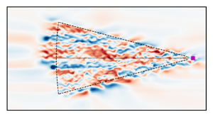
In the current work, we collect our measurements in plan-position-indicator (PPI) scanning mode with a zero elevation angle and constant azimuthal sweeping covering the horizontal sector shown in figure 1. The measurements are collected for a period of  $T_m=0.1 H/u_*$ from a single lidar mounted at $\boldsymbol {x}_m=[0,0,0.1H]$, with a range gate of $\Delta r=105$ m and total number of gates of $N_r=100$. Therefore, at each sampling time $t_n=t_0+nT_s$, with $T_s=5 \times 10^{-4}H/u_*=1$ s, a vector of wind-speed readings $\boldsymbol {y}_n=[y_{n,1},\ldots,y_{n,N_r}]$ is measured using ${y}_{n,i}={h}_{n,i}(\boldsymbol {u}({x}, t))$ and stored at equally spaced locations along the lidar beam. The observation function ${h}_{n,i}$ is given as (Bauweraerts & Meyers Reference Bauweraerts and Meyers2020)
 \begin{equation} h_{n, i}(\boldsymbol{u}(\boldsymbol{x}, t)) \triangleq \frac{1}{T_s} \int_{t_{n-1}}^{t_n} \int_{\varOmega} \boldsymbol{u}(\boldsymbol{x}, t) \boldsymbol{\cdot} \boldsymbol{e}_l(t) \mathcal{G}\left(\boldsymbol{Q}(t) \left(\boldsymbol{x}-\boldsymbol{x}_i(t)\right)\right)\, \mathrm{d}\kern0.7pt \boldsymbol{x}\, \mathrm{d}t, \end{equation}
where  $\mathcal {G}$ is the lidar filter kernel, $\boldsymbol {e}_l$ is the lidar beam direction, $\boldsymbol {Q}$ is a rotation matrix from the reference to the lidar coordinate system and $\boldsymbol {x}_i$ is the measurement location given as $\boldsymbol {x}_i(t)=\boldsymbol {x}_m+(r_0+\Delta r(i-1)) \boldsymbol {e}_l(t)$, with the lidar range gate $\Delta r=105$ m and $i=1, \ldots, N_r$. The lidar beam moves in a horizontal sweeping pattern with a constant azimuthal angular velocity of $|\partial \phi /\partial t|=2\Delta \phi /T_m=0.00371$ rad s $^{-1}$, where $\Delta \phi$ is the azimuthal range covered by the lidar. Figure 1 summarizes this picture.

Figure 1. Schematic of the reference (a) and reconstruction (b) domains with the lidar mount (purple) and the scanning region (inside dashed lines). The figure is reprinted from Bauweraerts & Meyers (Reference Bauweraerts and Meyers2020).
5.2. Set-up of reference simulation
In the current study, we assume a pressure-driven boundary layer with a height of  $H=1$ km, a friction velocity of $u_*=0.5$ m s $^{-1}$ and a roughness length of $z_0=0.1$ m. After a spin-up period of $50H/u_{*}$ on a reference domain $30H \times 5.4H \times H$ with a fine grid of size $2000 \times 360 \times 200$, a series of virtual measurements are collected in the PPI scanning mode over a period of $T_m=200$ s and also $400$ s. After obtaining the measurement series ${\boldsymbol{\mathsf{Y}}}$, the reconstruction problem can be started. The reconstruction is done on a shorter domain with a coarser mesh than the reference simulation. In this study, the reconstruction domain has dimensions of $18H \times 5.4H \times H$ with a grid size of $360 \times 108 \times 60$ (see figure 1). Before solving the optimization problem (2.4), the background correlation tensor $\hat {\boldsymbol {R}}$ is constructed from the analytical models in § 3 on the reconstruction grid and stored to be used as a prior for the MAP problem in (2.4). Computing and storing the analytical tensor takes only a few seconds using the same computational nodes allocated for the optimization problem (see § 5.4). Therefore, they are usually deleted after solving the optimization problem and recomputed again when needed.
5.3. Set-up of correlation tensor
5.3.1. The HGW model
As discussed above, the HGW correlation tensor in (3.6) is a function of the length scale  $\ell$ and the isotropic variance $\sigma _{iso}^2$. Meteorological data from the ABL (Kaimal et al. Reference Kaimal, Wyngaard, Izumi and Coté1972) show that the variances of the different velocity components $\sigma _{u}^2$, $\sigma _{v}^2$ and $\sigma _{w}^2$ in the surface layer (i.e. $x_3 \le 0.1H$) are not equal to each other (see table 1). However, because of the isotropic assumption in the HGW model, the model cannot pick up a preferred direction, meaning that only a single choice of the variance can be imposed. In this study, we choose the isotropic variance to be equal to the streamwise variance of Kaimal et al. (Reference Kaimal, Wyngaard, Izumi and Coté1972), leading to $\sigma _{iso}^2=4.77 u_*^2$. On the other hand, the length scale $\ell$ is chosen to match the inertial subrange asymptote (Peltier et al. Reference Peltier, Wyngaard, Khanna and Brasseur1996), which leads to the following expression (Wilson Reference Wilson1997):
 \begin{equation} \ell = 0.8743 \frac{\sigma_{iso}^3}{\epsilon}, \end{equation}
where  $\epsilon$ is the turbulent kinetic energy dissipation rate. Using the similarity theory in the surface layer of a neutrally stable ABL, the dissipation rate can be approximated as (Stull Reference Stull1988)
 \begin{equation} \epsilon=1.24 \frac{u_*^3}{\bar{\kappa} z}, \end{equation}
where  $\bar {\kappa } = 0.41$ and $z$ is the vertical distance, which is chosen to be equal to the lidar height $z=0.1H$. The resulting values of the parameters are summarized in table 3. It is worth mentioning that we noticed that the reconstruction results are not very sensitive to small changes in the model parameters.
Table 1. Values of velocity variances as given in Kaimal et al. (Reference Kaimal, Wyngaard, Izumi and Coté1972).

As briefly mentioned in § 3, the analytical IFT for the spectral tensor  ${\boldsymbol {\varPhi }}^{iso} (\boldsymbol {k})$ used in the HGW model is only available for the Batchelor turbulence case (see Appendix D), which is the main advantage of this model. Therefore, we limit our analysis for the HGW to the Batchelor case.
5.3.2. The Mann model
In addition to the two parameters discussed above ( $\sigma _{iso},\ell$), the Mann model has an additional parameter $\varGamma$ which reflects the amount of distortion applied to the initial isotropic tensor. If $\varGamma =0$, no shear is imposed and the isotropic tensor in (3.3) is retrieved. As $\varGamma$ is increased, $\sigma _{u}^2$ and $\sigma _{v}^2$ increase while $\sigma _{w}^2$ and $\sigma _{uw}$ decrease. This behaviour is illustrated in figure 4 of Mann (Reference Mann1994). To choose the model parameters, Mann used a least-squares fitting algorithm to match the one-dimensional spectra produced by the model to the ones obtained experimentally. Here, we use a simpler procedure, similar to the one reported by Wilson (Reference Wilson1998), that is also more in line with the typical data that would be available from atmospheric measurements. Firstly, using figure 2, $\varGamma$ is chosen to satisfy the ratio $\sigma _u^2/\sigma _w^2$ obtained from the reference LES at $x_3=0.1H$ (see table 2). Afterwards, $\varGamma$ and $\sigma ^2_u/u_*^2$ are used to obtain $\sigma _{iso}^2$ from figure 2. Finally, the length scale $\ell$ is obtained similarly to the previous section. Table 3 summarizes the parameters obtained following this procedure for both Batchelor and Saffman energy spectra.
Table 2. Values of velocity variances as calculated from the reference LES at  $x_3=0.1H$.

Table 3. Parameters of the spectral tensors in § 3.


Figure 2. The normalized velocity variance of the Mann model as  $\varGamma$ changes using Batchelor and Saffman energy spectra. The blue colour represents $\sigma _u^2/\sigma _{iso}^2$, while the red and green represent $\sigma _v^2/\sigma _{iso}^2$ and $\sigma _w^2/\sigma _{iso}^2$, respectively. The vertical dotted lines correspond to the selected $\varGamma$ values following the procedure in § 5.3.2 for both Batchelor and Saffman cases.
As will be described in § 5.4, the absolute value of  $\sigma _{iso}^2$ in table 3 becomes somehow redundant in our 4D-Var problem due to the Pareto front technique used to fix $\gamma ^2$. Nonetheless, we opted to propose a way to fix it as part of the parameter selection process in the current section.
5.3.3. Two-point correlation tensor
In this section, we compute the diagonal component of the normalized two-point correlation function in the streamwise direction, given as  $C_{11}(\boldsymbol {x},\boldsymbol {\breve {x}})= R_{11}(\boldsymbol {x},\boldsymbol {\breve {x}})/ \sigma ^2_{u}(\boldsymbol {x},\boldsymbol {\breve {x}})$, for both the Mann and the HGW models presented in § 3, and compare them with those obtained by Bauweraerts & Meyers (Reference Bauweraerts and Meyers2020) in figure 3.

Figure 3. Cross-section of the two-point correlation  $C_{11}(\boldsymbol {x},\boldsymbol {\breve {x}})$ with reference point $x = [0, 0, H/4]$ at $x_3 = H/4$ (b), $x_2 =0$ (a) and $x_1=0$ (c). The contour lines are drawn for $C_{11}=[-0.1,-0.05,0.05,0.1,0.3]$: solid black, $C>0$; dashed red, $C<0$. The figure is reprinted from Bauweraerts & Meyers (Reference Bauweraerts and Meyers2020).
Figures 4 and 6 present  $C_{11}$ for the HGW and Mann models, respectively, for a reference point located at $\boldsymbol {x}=[0,0,H/4]$, which is a bit higher than the lidar height in § 5.1. However, we opted to show the correlation function at this height to facilitate comparisons with figure 3. Moreover, the difference between the two heights is negligible (not shown). The figures provide a visual comparison of the correlation functions between the two models. For the HGW model with Batchelor spectrum (figure 4), the correlation consists of three small positive central lobes with a spanwise width close to what is observed in Bauweraerts & Meyers (Reference Bauweraerts and Meyers2020). However, the HGW model underpredicts the correlation length by an order of magnitude when compared with the value of $10H$ reported by Fang & Porté-Agel (Reference Fang and Porté-Agel2015) around the reference point.

Figure 4. Cross-section of the HGW two-point correlation  $C_{11}(\boldsymbol {x},\boldsymbol {\breve {x}})$ with reference point $x = [0, 0, H/4]$ at $x_3 = H/4$ (b), $x_2 =0$ (a) and $x_1=0$ (c).
On the other hand, the Mann model in figures 5 and 6 exhibits a more complex correlation function. In the horizontal plane, the function displays three closed lobes elongated in the  $x_1$ direction, with a size significantly larger than in the HGW case. However, it can be clearly seen that utilizing the Saffman spectrum (figure 6) leads to the longest correlations among the proposed models. In the spanwise direction, the correlation function decreases until it reaches a saturation point at a small negative value. In contrast, Bauweraerts & Meyers (Reference Bauweraerts and Meyers2020) observed long alternating positive and negative lobes extending throughout the entire domain in the streamwise direction, with a correlation width much less than the one observed here. These long lobes were attributed to the large-scale coherent structures in a neutral ABL as observed in Alcayaga et al. (Reference Alcayaga, Larsen, Kelly and Mann2020).

Figure 5. Cross-section of the Mann (with Batchelor spectrum) two-point correlation  $C_{11}(\boldsymbol {x},\boldsymbol {\breve {x}})$ with reference point $x = [0, 0, H/4]$ at $x_3 = H/4$ (b), $x_2 =0$ (a) and $x_1=0$ (c).

Figure 6. Cross-section of the Mann (with Saffman spectrum) two-point correlation  $C_{11}(\boldsymbol {x},\boldsymbol {\breve {x}})$ with reference point $x = [0, 0, H/4]$ at $x_3 = H/4$ (b), $x_2 =0$ (a) and $x_1=0$ (c).
In the  $x_2\unicode{x2013}x_3$ direction, we also observe central positive lobes. In the $x_1\unicode{x2013}x_3$ plane, the Mann model produces positive lobes that are inclined in the direction of the mean flow with an inclination angle of around $19^\circ$, which is slightly higher than what is observed in other studies (Marusic & Heuer Reference Marusic and Heuer2007; Sillero, Jiménez & Moser Reference Sillero, Jiménez and Moser2014), where a value of around $10^\circ$ was reported. We observed that the inclination is very sensitive to the choice of $\varGamma$. However, in the current work, we prioritize a practicable way of selecting parameters, as outlined in § 5.3.2, rather than further fitting on the inclination angle, which is not directly identifiable as an input to the prior in our 4D-Var formulation.
5.4. Set-up of the assimilation problem
After determining the correlation tensor in the previous section, one remaining component to be chosen before solving the optimization problem (2.4) is the variance  $\gamma ^2$. Looking at the optimization problem, the objective function can be rewritten in a more explicit way as $\mathscr {J}(\boldsymbol {\varTheta }_0)=\boldsymbol{\varTheta} _0^T \boldsymbol {B'}^{-1} \boldsymbol {\varTheta }_0/2\sigma _{iso}^2+ \sum _{n=1}^{N_s} \| \boldsymbol {y}_n-\boldsymbol {h}_n(\mathcal {M}_t(\mathcal {R}(\boldsymbol {\varTheta }_0)) \|^2 / 2 \gamma ^2$, where $\boldsymbol {B'}$ is the normalized correlation tensor. As can be noticed, the relative weight of each term with respect to the other is determined by the ratio $\gamma ^2/\sigma _{iso}^2$, instead of the individual values of $\gamma ^2$ and $\sigma _{iso}^2$. However, since $\sigma _{iso}^2$ was already fixed in § 5.3 as part of the parameter selection procedure, $\gamma ^2$ now serves as the only weighting parameter between the two terms in the cost function, and the absolute value of $\sigma ^2_{iso}$ becomes somehow redundant. For a fixed $\sigma ^2_{iso}$, as $\gamma ^2$ is increased, less trust is given to the likelihood term, leading to a smoother solution. Decreasing $\gamma ^2$ gives more significance to the likelihood term, and the obtained solution becomes more irregular. In order to choose a suitable value for $\gamma ^2$, a trade-off between solution complexity and smoothness needs to be achieved. Similarly to Bauweraerts & Meyers (Reference Bauweraerts and Meyers2020), this is done through Pareto front analysis, which requires solving the optimization problem multiple times per model for different values of $\gamma ^2$. Figure 7 shows that $\gamma ^2=10^{-3}$ achieves a good trade-off for both models, so it will be used in the rest of this study. According to our experience, the reconstruction accuracy appears to be much more sensitive to big changes in $\gamma ^2$ than the convergence behaviour.

Figure 7. Pareto front for the optimization problem (2.4) using the HGW (a) and Mann regularization with Batchelor spectrum (b). The figure is obtained by solving the optimization problem many times using different values of  $\gamma ^2$. The points are labelled with the corresponding $\gamma ^2$ value.
After choosing  $\gamma ^2$, the optimization problem (2.4) is solved for an optimization time horizon equivalent to the lidar scanning period $T_m$, with an initial condition $\hat {{\boldsymbol {\varTheta }}}_0=0$. The spatial mean flow profile of the initial field as well as the surface roughness and $u_*$ are assumed to be known from the reference simulation. Starting from the initial condition, the optimization algorithm converges to a local minimum where $\boldsymbol {\nabla } \mathscr {J}=0$. In this study, the optimization algorithms stop upon achieving a relative value of the gradient norm $\| \boldsymbol {\nabla } \mathscr {J} \| / \| \boldsymbol {\nabla } \mathscr {J}_0 \|=6 \times 10^{-3}$, where $\boldsymbol {\nabla } \mathscr {J}_0$ is the initial gradient obtained using an initial guess for the initial condition $\hat {{\boldsymbol {\varTheta }}}_0=0$. Figures 8 and 9 show the convergence history of the HGW and Mann models with the Batchelor spectrum. Each iteration corresponds to an L-BFGS-B iteration, which involves a forward and adjoint simulation as well as a line search procedure (if the initial step $\alpha _k$ does not satisfy the Wolfe conditions). However, we only needed to perform the additional line search procedure a few times, so the total number of iterations mainly represents the number of forward simulations (or half of the forward and adjoint simulations). Figure 9 shows that we achieve a super-linear convergence rate when either of the analytical models is used.

Figure 8. Cost function convergence (100 iterations) using the HGW (a) and Mann regularization with Batchelor spectrum (b).

Figure 9. Convergence of the relative gradient using the HGW regularization (blue) and Mann regularization with Batchelor spectrum (orange).
As a point of comparison, we also investigated ridge regression. We found that it leads to slow convergence (a slope of  $-1.1$), and only provides reasonable results inside the scanning area, as further discussed in Appendix E. We will use results from the ridge regression as a further point of comparison in the reconstruction error analysis discussed in § 6.2.
The optimization in this study was performed on the wICE supercomputer of the Flemish supercomputer centre using four computational nodes, each of which has two Intel Xeon Platinum 8360Y 2.4 GHz CPUs with 256 GB RAM. The total wall time of one assimilation problem with  $T_m=0.1H/u_*$ (provided 100 iterations) is around 8 hours. It must be highlighted that this cost includes the preprocessing cost (involving the computation of the background tensor), which is negligible in our assimilation algorithm compared with the previous study of Bauweraerts & Meyers (Reference Bauweraerts and Meyers2020).
6. Results
In this section, the reconstructed turbulent velocity field is visualized, and the results are compared with the reference field from which the virtual lidar measurements were collected.
6.1. Single assimilation window
We first discuss the results of a single assimilation window with an assimilation horizon of  $T_m=0.1H/u_*$ using the analytical models described in § 3. Figure 10 presents a comparison between the reconstructed velocity fluctuations and the reference values obtained using two different models: the HGW model with a Batchelor spectrum and the Mann model with a Saffman spectrum. Similar plots were also generated for the Mann model with a Batchelor spectrum, but those are not shown here as they are not significantly different from the Saffman case. The results are shown at the beginning $(t=t_i)$ and the end $(t=t_f)$ of the assimilation window for vertical and horizontal cross-sections at $x_2=0$ and $x_1=0.1H$, respectively. Inside the scanning area, both models show good reconstruction accuracy in figure 10(g–l). Additionally, some fluctuations were also captured in small regions upstream and downstream of the scanning area due to the horizontal transport by the mean flow (Bauweraerts & Meyers Reference Bauweraerts and Meyers2020). Away from the scanning region, the likelihood term in the optimization problem (2.4) vanishes due to the absence of any measurements, and the only remaining contribution in the MAP problem is due to the initial background distribution provided by the analytical models.

Figure 10. The streamwise velocity fluctuation component at the  $x_2=0$ (a–f) and $x_3=0.1H$ (g–l) planes. The right column is the reference velocity and the left two columns are the reconstructed velocities using the HGW model and the Mann model (with Saffman spectrum), respectively. Panels (a–c) and (g–i) show the velocity at $t=0$, while (d–f) and (j–l) show the velocity at $t=0.1H/u_*$. The dashed lines represent the boundaries of the scanning area, and the solid line represents the lidar beam.
For the vertical section in figure 10(a–f), the lidar measurements are available only at a height of  $x_3=0.1H$. The mean velocity in the vertical direction is zero, so that no mean advection in that direction occurs. Therefore, the small structures are reconstructed only in small local regions around the lidar beam. However, due to the decaying correlations in the vertical direction provided by the analytical models, large structures are reconstructed up to a height of approximately $x_3=0.7H$. These observations agree with the results obtained in figures 4–6. Owing to the isotropic assumption in the HGW model, no inclination in the reconstructed fluctuations in the vertical direction is observed, whereas in the Mann model the inclination in the direction of the mean flow can be clearly seen.
To more closely examine the accuracy of the velocity reconstruction in the scanning area, we compare the reference and reconstructed streamwise velocity components for different sections at the middle of the assimilation window ( $t=0.05H/u_*$) in figure 11. At the lidar height ( $x_3=0.1H$), both models exhibit very good agreement between the reference and reconstructed velocity components. However, as the height increases, the reconstruction accuracy gradually decreases, as expected from the earlier discussion. On the other hand, the reconstruction closer to the wall is accurate only for the large and not the small scales, which is expected from figures 4–6. This observation is seen to be true for both models, as seen in figure 11.

Figure 11. Comparison between the reconstructed velocity using the HGW model (green), the reconstructed velocity using the Mann model with Saffman spectrum (orange) and the reference velocity (blue) for the streamwise component at different lines in the vertical direction. The measurements are taken at  $t=0.05H/u_*$.
6.2. Error statistics
In this section, the statistics of the error in the reconstructed streamwise velocity component are studied. To this end, we define two metrics based on the instantaneous reconstruction error for the streamwise velocity component  $\epsilon (\boldsymbol {x},t)=I_{c}^{f}(u_1(\boldsymbol {x},t))- u_{1,{ref}}(\boldsymbol {x},t)$, where $u_1$ is the reconstructed velocity, $u_{1,{ref}}$ is the reference velocity and $I_{c}^{f}$ represents interpolation from the coarse reconstruction to the fine reference grid.
In order to facilitate a direct comparison with the results of the reconstruction method based on proper orthogonal decomposition (POD) presented in Bauweraerts & Meyers (Reference Bauweraerts and Meyers2020), we define, in a first step, the spatially averaged error  $\langle ( \epsilon (\boldsymbol {x},t)) ^2 \rangle _{\varGamma }$, where $\varGamma$ is the horizontal area swept by the lidar beam after truncating one convective distance $U_{\infty }T$ to avoid boundary effects. In figure 12, we present a comparison of the normalized spatially averaged errors of the HGW, Mann (Saffman) and simple ridge regression models and the POD-based reconstruction errors reported in Bauweraerts & Meyers (Reference Bauweraerts and Meyers2020). The horizontal dashed line represents the reconstruction using the mean flow only, with (given the normalization by $\langle u_{1,{ref}}^{\prime 2} \rangle _{\varGamma }$) a corresponding value of 1. Examining figure 12(a) reveals that the ridge regression regularization results in an acceptable accuracy only within the scanning region, corroborating the findings detailed in Appendix E. In contrast, using either the HGW or Mann regularization yields a reconstruction accuracy closer to that achieved by the considerably more resource-intensive POD-based approach. In figure 12(b), errors are depicted over time at the lidar height $x_3=0.1H$. Notably, both the HGW and the Mann models show highly satisfactory reconstruction accuracy, closely rivalling that of the POD approach. The ridge regression reconstruction exhibits larger errors at the start of the assimilation window that decrease gradually with time. In alignment with observations from Bauweraerts & Meyers (Reference Bauweraerts and Meyers2020), optimal reconstruction results are consistently achieved at the midpoint of the assimilation window for all models considered. Further insights into this phenomenon will be explored in § 6.3.

Figure 12. The normalized spatially averaged error inside the scanning area for the ridge, HGW and Mann (Saffman) models and the POD-based regularization in Bauweraerts & Meyers (Reference Bauweraerts and Meyers2020). Panel (a) shows the errors at  $t=0.05u_*/H$, while (b) shows the results at $x_3=0.1H$. The horizontal dashed line represents estimation with the mean flow, which leads to an expected error of $\langle \epsilon ^2\rangle _{\varGamma } =\langle u_{1, {ref}}^{\prime 2}\rangle _{\varGamma }$.
We now further focus on a detailed error comparison by introducing a second metric, namely the mean-squared error (MSE) of the reconstructed velocity, which can be defined as
 \begin{equation} MSE(\boldsymbol{x})=\langle \langle \epsilon ^2(\boldsymbol{x},t)\rangle_T \rangle_e, \end{equation}
where  $\langle {\cdot } \rangle _e$ and $\langle {\cdot } \rangle _T$ denote the ensemble average and time average, respectively. Furthermore, the error metric is normalized using the background variance $\langle \langle u'^2_{1,{ref}}\rangle _T \rangle _e$ similar to the above. The normalized mean-squared error (NMSE) can then be defined as $NMSE(\boldsymbol {x})={MSE(\boldsymbol {x})}/{ \langle \langle u'^2_{1,{ref}} \rangle _T \rangle _e}$. Figure 13 shows sections of the NMSE for the reconstructed streamwise velocity component considering 10 different assimilation windows (with a time horizon of $T=200$ s) to compute the ensemble average for each model in § 3, while the time average is performed over each assimilation window. The NMSE is computed based on three different models: the HGW model (figure 13a,d), the Mann model with Batchelor spectrum (figure 13b,e) and the Mann model with Saffman spectrum (figure 13c,f). Within the scanning region in the horizontal plane, all models exhibit a high level of accuracy in reconstructing the flow. However, outside the scanning area, the accuracy drops significantly for the Mann model with Batchelor spectrum in the streamwise direction compared with the other two models. Nevertheless, using the Saffman instead of the Batchelor spectrum reduces these errors, as seen in the figure. This can be attributed to the fact that the Saffman spectrum leads to longer positive correlations in the longitudinal direction compared with the Batchelor spectrum, as discussed in § 5.3.3. We further looked at energy spectra over the domain width and over the different reconstruction windows (not shown here), observing that, indeed, the Saffman case has much more energy in the large scales. In the regions further away from the measurement area, the NMSE is close to 1, which indicates that the model is not able to predict any turbulent features, which is a logical result of the lack of measurements in this region.

Figure 13. The NMSE of the reconstructed streamwise velocity component at  $x_3=0.1H$ using the HGW regularization (a,d), the Mann regularization with Batchelor spectrum (b,e) and the Mann regularization with Saffman spectrum (c,f).
In the vertical direction, figure 13(a–c) demonstrates a marginal improvement in the reconstruction accuracy close to the lidar height for the Mann model using either of the energy spectra compared with the HGW case, but these differences may fall within the averaging accuracy.
It is important to note that obtaining a high reconstruction accuracy far away from the scanning region is not the primary goal of the data assimilation problem. In fact, this region is usually filtered out in practice to end up with only the region of interest (i.e. the scanning area, possibly slightly extended to incorporate effects of advection in the reconstruction). While the correlation function plays a major role (filling the gaps) inside the region of interest by correlating the scalar speed measurements to their surroundings, the absence of such a correlation function leads to an undetermined system, even inside the measurement area. Moreover, the accuracy outside can be also enhanced by considering a more realistic mean flow, as will be discussed in § 7.
6.3. Effect of the time horizon (HGW model)
In this section, we investigate the influence of the time horizon on the accuracy of reconstruction. We replicate the analysis presented in § 6.1 for two distinct windows characterized by different assimilation horizons  $T_p$ using the HGW model. The first window spans a time interval of $200$ s, commencing at $t_i=t_f-200$ s. Meanwhile, the second window covers a wider period of $400$ s, initiating at $t_i=t_f-400$ s. Here, $t_f$ represents a specific time instant. Increasing the time horizon further leads to divergence of the adjoint solution due to the chaotic nature of turbulence. Therefore, we limit our analysis to these two windows. Figure 14(f–h) show three snapshots of the reference field at $t=t_f-400$ s, $t=t_f-200$ s and $t=t_f$, respectively. The reconstructed field for the short and long assimilation windows is shown in figure 14(a,b) and 14(c–e), respectively. Moreover, the instantaneous reconstruction error is shown in figure 14(i–k) and 14(l,m) for the long and short assimilation windows, respectively.

Figure 14. The reconstructed streamwise velocity field at  $x_3=0.1H$ using the HGW model at $t=t_f$ and $t=t_f-200$ s (a,b) for an assimilation window of $T_s=200$ s, and at $t=t_f-400$ s, $t=t_f-200$ s and $t=t_f$ for an assimilation window of $T_s=400$ s (c–e). The corresponding instantaneous reconstruction error is also shown in (i–m). In (f–h) snapshots of the reference field are shown.
At  $t=t_f-200$ s, it can be clearly seen that the reconstruction accuracy is significantly increased when the time instant is located at the middle of the assimilation window, as seen in figure 14(j), compared with the initial instant for the short window in figure 14(l). On the other hand, the accuracy at the final instant $t=t_f$ for both windows in figure 14(k,m) are seen to be nearly the same as each other, and lower when compared with the reconstruction of the long window at $t=t_f-200$ s.
7. Conclusion and future perspectives
In this paper, we reconstructed the turbulent flow field in a neutrally stratified ABL using a strong 4D-Var assimilation approach combined with an LES model. Whilst this problem was tackled before by Bauweraerts & Meyers (Reference Bauweraerts and Meyers2020), the focus in the current study was on providing a more practical, fast and cost-effective assimilation algorithm. To this end, we formulated our problem in a solenoidal space to enforce the continuity equation and regularized it using two fast analytical approximations for the background covariance tensor. The problem was then preconditioned using the analytical tensor to increase the convergence rate, which resulted in a super-linear convergence to a local minimum.
The error study revealed that regularizing the MAP problem with either the HGW or the Mann model (with Saffman spectrum) yields favourable reconstruction accuracy. However, it is worth noting that the HGW model has limitations in capturing the shear profile, leading to errors in the vertical direction close to the lidar plane when compared with the Mann model. This limitation may become particularly significant in scenarios where there is strong shear present, but in the current work the difference between the HGW and Mann (with Saffman) models was rather small. Furthermore, for the Mann model, the error study revealed the sensitivity of the reconstruction accuracy to the length of the correlation function in the streamwise direction. The Saffman energy spectrum, characterized by a slower decay as  $k \rightarrow 0$, allows for the representation of longer structures when employed in the Mann model. In contrast, the Batchelor case exhibits a faster decay. The ability to represent longer structures with the Saffman spectrum can be advantageous in capturing larger-scale features in the flow.
In the current work, we also studied the effect of increasing the assimilation time horizon on the reconstruction accuracy. The study showed that in a strong 4D-Var method, the best reconstruction accuracy is obtained at the middle of the assimilation window rather than the terminal time, which can be attributed to the fact that the error history of the MAP estimate is not included in the case of the strong 4D-Var. Formulating a weak 4D-Var such that the maximum accuracy is obtained at the final time can be of particular significance, especially in applications such as optimal control.
In this study, we limited our analysis to the neutrally stratified ABL. Extending the analysis to other stability conditions should be possible. For instance, the modified Mann model in Chougule et al. (Reference Chougule, Mann, Kelly and Larsen2018) can be used to regularize the temperature fluctuations alongside the velocity fluctuations in a stable ABL. Furthermore, it is possible to relax the assumption of a known mean flow by estimating both the initial mean profile and the fluctuation field. However, this estimation process requires obtaining the statistical properties of the mean flow, including its direction and magnitude, in addition to the turbulent part. One approach to achieve this is by, for example, using a hierarchical Bayesian analysis, in which the mean flow is first included (e.g. using weather models) and the turbulent field is then included at a lower level.
The focus of the current study was on assessing the possibility of directly applying the HGW and Mann models within a reconstruction algorithm. However, further development of an analytical model that is able to more precisely represent the significant structural characteristics such as the meandering behaviour can be valuable (Hutchins & Marusic Reference Hutchins and Marusic2007).
Finally, extending the time horizon in this analysis revealed promising results that can be further explored by further increasing the time horizon. While this is not possible using the current single shooting approach due to the chaotic divergence of the LES model, novel techniques such as multiple shooting can be used for this purpose.
Acknowledgements
The first author thanks L. Fang for insightful discussions.
Funding
The authors acknowledge support from the KU Leuven research council, grant number C16/17/008, and from the project BeFORECAST, funded by the Energy Transition Funds of the Federal Public Service Economy of the Belgian Federal Government.
Declaration of interests
The authors report no conflict of interest.
Appendix A. State space model
A.1. Governing equations
The neutrally stratified ABL flow considered in this manuscript is modelled through the incompressible Navier–Stokes equations and solved using a standard LES strategy. This model was described in detail in many previous articles (e.g. Munters, Meneveau & Meyers Reference Munters, Meneveau and Meyers2016; Bauweraerts & Meyers Reference Bauweraerts and Meyers2020). Nevertheless, it will be briefly discussed here for completeness. The filtered incompressible Navier–Stokes momentum and continuity equations are given as
 \begin{equation} \left.\begin{array}{c@{}} \displaystyle \dfrac{\partial \tilde{\boldsymbol{u}}}{\partial t}+(\tilde{\boldsymbol{u}} \boldsymbol{\cdot} \boldsymbol{\nabla}) \tilde{\boldsymbol{u}}={-}\dfrac{1}{\rho}\boldsymbol{\nabla}(p_{\infty}+\tilde{p})-\boldsymbol{\nabla} \boldsymbol{\cdot} \boldsymbol{\tau}_{\!sgs} ,\\ \boldsymbol{\nabla} \boldsymbol{\cdot} \tilde{\boldsymbol{u}}=0, \end{array}\right\} \end{equation}
where  $\tilde {\boldsymbol {u}}$ is the filtered velocity at the grid scale, $\boldsymbol {\nabla } p_{\infty }$ is the mean pressure gradient given as $\boldsymbol {\nabla } p_{\infty }=[-u_{*}^2 H^{-1}, 0,0]$ and $\tilde {p}$ is the filtered pressure fluctuation. The standard constant-coefficient Smagorinsky model (Smagorinsky Reference Smagorinsky1963) is used to model the deviatoric part of the subgrid-scale stress tensor with $C_s=0.14$, combined with wall damping (Mason & Thomson Reference Mason and Thomson1992) to avoid excessive dissipation of kinetic energy with $n=1$. The trace of the stress tensor $\boldsymbol {\tau }_{\!sgs}$ is absorbed into the filtered pressure $\tilde {p}$ as a common practice in incompressible LES.
In this paper, all simulations are done on a computational domain that has periodic boundary conditions in the horizontal plane. Therefore, the domain length is made sufficiently large to prevent any boundary effects on the solution in the domain of interest. In the vertical direction, an impermeable wall stress boundary condition is used following Bou-Zeid, Meneveau & Parlange (Reference Bou-Zeid, Meneveau and Parlange2005). At the top boundary, the vertical motion is blocked by an impermeable slip boundary condition. The governing equations are discretized using the Fourier pseudospectral method described in § A.2 and solved using our in-house LES code SP-Wind (Meyers & Sagaut Reference Meyers and Sagaut2007; Munters et al. Reference Munters, Meneveau and Meyers2016).
A.2. Discretization
Using the horizontal homogeneity assumption and the truncated discrete Fourier analysis, the components of the discrete velocity vector  $\boldsymbol {U}$ defined in § 2 can be expressed as
 \begin{equation} {U}_{mn}^{j} =\sum_{p_{{min}={-}N_1/2}}^{p_{{max}=(N_1/2-1)}} \sum_{q_{{min}={-}N_2/2}}^{q_{{max}=(N_2/2-1)}} {\hat{U}}_{pq}^{j} \exp \left({\rm i} 2{\rm \pi} \left(\frac{pn}{N_1} +\frac{qm}{N_2}\right)\right),\end{equation}
where  ${U}_{mn}^{j}$ has a length of $N_3$ when $j=1,2$ and $N_3-1$ when $j=3$. Here, $m$ and $n$ are indices corresponding to horizontal spatial locations such that $x_1=mL_1/N_1$ and $x_2=nL_2/N_2$. Further, ${\hat {U}}_{pq}^{j}$ is the complex-valued Fourier coefficient of the Fourier mode with streamwise wavenumber $k_1=2{\rm \pi} p/L_1$ and spanwise wavenumber $k_2=2{\rm \pi} q/L_2$. Rewriting the latter equation in matrix form for the three velocity components, including all grid points in the vertical direction, gives
 \begin{equation} \left.\begin{array}{@{}c@{}}
\left[\begin{array}{@{}c@{}} {U}_{mn}^{1}(t) \\ {U}_{mn}^{2}(t)
\\ {U}_{mn}^{3}(t) \end{array}\right]
=\left[\begin{array}{@{}ccc@{}} {\mathcal{W}}^1 & \boldsymbol{0}
& \boldsymbol{0} \\ \boldsymbol{0} & {\mathcal{W}}^2 &
\boldsymbol{0} \\ \boldsymbol{0} & \boldsymbol{0} &
{\mathcal{W}}^3 \\ \end{array}\right]
\left[\begin{array}{@{}c@{}} \hat{\boldsymbol{U}}^1(t) \\
\hat{\boldsymbol{U}}^2(t) \\ \hat{\boldsymbol{U}}^3(t)
\end{array}\right], \\ \boldsymbol{U}_{mn}(t) =
\boldsymbol{\mathcal{W}}
\boldsymbol{\hat{\boldsymbol{U}}}(t),
\end{array}\right\} \end{equation}
\begin{equation} \left.\begin{array}{@{}c@{}}
\left[\begin{array}{@{}c@{}} {U}_{mn}^{1}(t) \\ {U}_{mn}^{2}(t)
\\ {U}_{mn}^{3}(t) \end{array}\right]
=\left[\begin{array}{@{}ccc@{}} {\mathcal{W}}^1 & \boldsymbol{0}
& \boldsymbol{0} \\ \boldsymbol{0} & {\mathcal{W}}^2 &
\boldsymbol{0} \\ \boldsymbol{0} & \boldsymbol{0} &
{\mathcal{W}}^3 \\ \end{array}\right]
\left[\begin{array}{@{}c@{}} \hat{\boldsymbol{U}}^1(t) \\
\hat{\boldsymbol{U}}^2(t) \\ \hat{\boldsymbol{U}}^3(t)
\end{array}\right], \\ \boldsymbol{U}_{mn}(t) =
\boldsymbol{\mathcal{W}}
\boldsymbol{\hat{\boldsymbol{U}}}(t),
\end{array}\right\} \end{equation}
where  ${\hat {\boldsymbol {U}}^j} =[\hat {U}^j_{p_{min} q_{min}}, \ldots,\hat {U}^j_{p_{max}q_{max}}]^T$ and ${\mathcal {W}^j}$ is a block matrix of inverse discrete Fourier transform sub-matrices in the horizontal plane and has a size of $N_1 N_2 N_3 \times N_1 N_2 N_3$ when $j=1,2$ and $N_1 N_2 (N_3-1) \times N_1 N_2 (N_3-1)$ when $j=3$. The second line of (A3) is a compact representation of the discretization.
Appendix B. Adjoint model
As already mentioned in § 4, the gradient in the current study is obtained using the continuous adjoint method derived in Goit & Meyers (Reference Goit and Meyers2015) and Bauweraerts & Meyers (Reference Bauweraerts and Meyers2020). The resulting adjoint equation can be written as
 \begin{equation} \left.\begin{array}{c@{}}
\displaystyle -\dfrac{\partial \boldsymbol{\zeta}}{\partial
t}=\tilde{\boldsymbol{u}} \boldsymbol{\cdot}
\boldsymbol{\nabla} \boldsymbol{\zeta}+\boldsymbol{\zeta}
\boldsymbol{\cdot} \boldsymbol{\nabla}
\tilde{\boldsymbol{u}}+\boldsymbol{\nabla}
\boldsymbol{\cdot} \boldsymbol{\tau}_{S G
S}^*+\dfrac{1}{\rho} \boldsymbol{\nabla}
{\rm \pi}+\sum_{i=1}^{N_r} \boldsymbol{f}_{\!i},\\
\boldsymbol{\nabla} \boldsymbol{\cdot}
\boldsymbol{\zeta}=0, \end{array}\right\}
\end{equation}
\begin{equation} \left.\begin{array}{c@{}}
\displaystyle -\dfrac{\partial \boldsymbol{\zeta}}{\partial
t}=\tilde{\boldsymbol{u}} \boldsymbol{\cdot}
\boldsymbol{\nabla} \boldsymbol{\zeta}+\boldsymbol{\zeta}
\boldsymbol{\cdot} \boldsymbol{\nabla}
\tilde{\boldsymbol{u}}+\boldsymbol{\nabla}
\boldsymbol{\cdot} \boldsymbol{\tau}_{S G
S}^*+\dfrac{1}{\rho} \boldsymbol{\nabla}
{\rm \pi}+\sum_{i=1}^{N_r} \boldsymbol{f}_{\!i},\\
\boldsymbol{\nabla} \boldsymbol{\cdot}
\boldsymbol{\zeta}=0, \end{array}\right\}
\end{equation}
with
 \begin{equation} \boldsymbol{f}_{\!i}=\frac{1}{\gamma^2 T_s} \sum_{n=1}^{N_s}(\kern0.7pt y_{n, i}-h_{n, i}) \mathcal{G}(\boldsymbol{Q}(t)(\boldsymbol{x}-\boldsymbol{x}_i(t))) \boldsymbol{e}_l(t) H\left(\frac{T_s}{2}-|t-t_{n-1 / 2}|\right), \end{equation}
where  $\boldsymbol {\zeta }$ and ${\rm \pi}$ are the adjoint velocity and pressure, respectively. Further, $\boldsymbol {\tau }_{S G S}^*$ is the adjoint subgrid-scale model. The adjoint equation is discretized and solved backward in time similarly to the forward model, starting from the terminal condition $\boldsymbol {\zeta }(\boldsymbol {x},t_f)=0$. The adjoint solution at the beginning of the assimilation window $\boldsymbol {\zeta }(\boldsymbol {x},0)$ is then used to compute the gradient using (4.1).
Appendix C. Projection and reconstruction operations
In this section, the projection and reconstruction operators in § 2 are derived in the Fourier space. Assuming incompressibility, the continuity equation in the horizontal wavenumber space can be written as
 \begin{equation} {0} = {\rm i} k_1 {\hat{U}}_{pq}^{1}+{\rm i} k_2 {\hat{U}}_{pq}^{2} +\boldsymbol{D}_z {\hat{U}}_{pq}^{3}, \end{equation}
where  $\boldsymbol {D}_z$ is a discretization matrix in the vertical direction of size $N_3 \times (N_3-1)$. Similarly, the vertical component of the vorticity is given as
 \begin{equation} \hat{\varOmega}^3_{pq}={-}{\rm i} k_2 {\hat{U}}_{pq}^{1}+{\rm i} k_1{\hat{U}}_{pq}^{2}.\end{equation}
 Writing (C2) for all wavenumbers (except the DC mode, i.e.  $(k_1,k_2)=(0,0)$) in matrix form, we get
 \begin{equation} \left.\begin{array}{@{}c@{}}
\left[\begin{array}{@{}ccc@{}} \boldsymbol{0} & \boldsymbol{0} &
\boldsymbol{I} \\ \boldsymbol{B} & \boldsymbol{C} &
\boldsymbol{0} \end{array}\right]\left[\begin{array}{@{}c@{}}
\hat{\boldsymbol{U}}^1 \\ \hat{\boldsymbol{U}}^2 \\
\hat{\boldsymbol{U}}^3 \end{array}\right]
=\left[\begin{array}{@{}c@{}} \hat{\boldsymbol{U}}^3 \\
\hat{\boldsymbol{\varOmega}}^3 \\ \end{array}\right],\\
\hat{\mathcal{P}}{\hat{\boldsymbol{U}}}=
\hat{\boldsymbol{\varTheta}},
\end{array}\right\},\end{equation}
\begin{equation} \left.\begin{array}{@{}c@{}}
\left[\begin{array}{@{}ccc@{}} \boldsymbol{0} & \boldsymbol{0} &
\boldsymbol{I} \\ \boldsymbol{B} & \boldsymbol{C} &
\boldsymbol{0} \end{array}\right]\left[\begin{array}{@{}c@{}}
\hat{\boldsymbol{U}}^1 \\ \hat{\boldsymbol{U}}^2 \\
\hat{\boldsymbol{U}}^3 \end{array}\right]
=\left[\begin{array}{@{}c@{}} \hat{\boldsymbol{U}}^3 \\
\hat{\boldsymbol{\varOmega}}^3 \\ \end{array}\right],\\
\hat{\mathcal{P}}{\hat{\boldsymbol{U}}}=
\hat{\boldsymbol{\varTheta}},
\end{array}\right\},\end{equation}
with
 \begin{equation} {\hat{\boldsymbol{\varOmega}}^3} =\left[\hat{\varOmega}^3_{p_{min}q_{min}}, \ldots,\hat{\varOmega}^3_{p_{max}q_{max}} \right]^T \quad \forall \, (p,q)\neq(0,0), \end{equation}
where  $\hat {\mathcal {P}}$ is a linear projection operator and
 \begin{align} \boldsymbol{B} =
\left[\begin{array}{@{}ccc@{}} -{\rm i} k_{2, min }
\boldsymbol{I}_{_{N_3 \times N_3}} & \ldots &
\boldsymbol{0}_{_{N_3 \times N_3}} \\ \vdots & \ddots &
\vdots \\ \boldsymbol{0}_{_{N_3 \times N_3}} & \ldots &
-{\rm i} k_{2, max } \boldsymbol{I}_{_{N_3 \times N_3}}
\end{array} \right],\quad \boldsymbol{C} =
\left[\begin{array}{@{}ccc@{}} {\rm i} k_{1, min}
\boldsymbol{I}_{_{N_3 \times N_3}} & \ldots &
\boldsymbol{0}_{_{N_3 \times N_3}} \\ \vdots & \ddots &
\vdots \\ \boldsymbol{0}_{_{N_3 \times N_3}} & \ldots &
{\rm i} k_{1, max} \boldsymbol{I}_{_{N_3 \times N_3}}
\end{array} \right].
\end{align}
\begin{align} \boldsymbol{B} =
\left[\begin{array}{@{}ccc@{}} -{\rm i} k_{2, min }
\boldsymbol{I}_{_{N_3 \times N_3}} & \ldots &
\boldsymbol{0}_{_{N_3 \times N_3}} \\ \vdots & \ddots &
\vdots \\ \boldsymbol{0}_{_{N_3 \times N_3}} & \ldots &
-{\rm i} k_{2, max } \boldsymbol{I}_{_{N_3 \times N_3}}
\end{array} \right],\quad \boldsymbol{C} =
\left[\begin{array}{@{}ccc@{}} {\rm i} k_{1, min}
\boldsymbol{I}_{_{N_3 \times N_3}} & \ldots &
\boldsymbol{0}_{_{N_3 \times N_3}} \\ \vdots & \ddots &
\vdots \\ \boldsymbol{0}_{_{N_3 \times N_3}} & \ldots &
{\rm i} k_{1, max} \boldsymbol{I}_{_{N_3 \times N_3}}
\end{array} \right].
\end{align}
To retrieve the velocity field, the continuity equation (C1) is added to the system (C3) and then the system is inverted to obtain the inverse transformation (for  $(k_1,k_2)\ne\, (0,0)$)
 \begin{equation} \boldsymbol{\hat{U}} =\hat{\mathcal{R}} \hat{{\boldsymbol{\varTheta}}},\end{equation}
with  $\hat {\mathcal {R}}$ the reconstruction operator
 \begin{equation} \hat{\mathcal{R}} =
\frac{1}{\kappa_i^2} \left[\begin{array}{@{}cc@{}} \boldsymbol{E}
& \boldsymbol{B} \\ \boldsymbol{F} & \boldsymbol{C}\\
\kappa_i^2 \boldsymbol{I} & \boldsymbol{0}
\end{array}\right], \end{equation}
\begin{equation} \hat{\mathcal{R}} =
\frac{1}{\kappa_i^2} \left[\begin{array}{@{}cc@{}} \boldsymbol{E}
& \boldsymbol{B} \\ \boldsymbol{F} & \boldsymbol{C}\\
\kappa_i^2 \boldsymbol{I} & \boldsymbol{0}
\end{array}\right], \end{equation}
where  $\kappa _i=(k_{1,i}^2+k_{2,i}^2)^{1/2}$ and
 \begin{align} \boldsymbol{E} =
\left[\begin{array}{@{}ccc@{}} -{\rm i} k_{1, min }
\boldsymbol{D}_z & \ldots & \boldsymbol{0}_{_{N_3 \times
N_3-1}} \\ \vdots & \ddots & \vdots \\
\boldsymbol{0}_{_{N_3 \times N_3-1}} & \ldots & -{\rm i}
k_{1, max } \boldsymbol{D}_z \end{array} \right], \quad
\boldsymbol{F} = \left[\begin{array}{@{}ccc@{}} -{\rm i} k_{2,
min } \boldsymbol{D}_z & \ldots & \boldsymbol{0}_{_{N_3
\times N_3-1}} \\ \vdots & \ddots & \vdots \\
\boldsymbol{0}_{_{N_3 \times N_3-1}} & \ldots & -{\rm i}
k_{2, max } \boldsymbol{D}_z \end{array}
\right].
\end{align}
\begin{align} \boldsymbol{E} =
\left[\begin{array}{@{}ccc@{}} -{\rm i} k_{1, min }
\boldsymbol{D}_z & \ldots & \boldsymbol{0}_{_{N_3 \times
N_3-1}} \\ \vdots & \ddots & \vdots \\
\boldsymbol{0}_{_{N_3 \times N_3-1}} & \ldots & -{\rm i}
k_{1, max } \boldsymbol{D}_z \end{array} \right], \quad
\boldsymbol{F} = \left[\begin{array}{@{}ccc@{}} -{\rm i} k_{2,
min } \boldsymbol{D}_z & \ldots & \boldsymbol{0}_{_{N_3
\times N_3-1}} \\ \vdots & \ddots & \vdots \\
\boldsymbol{0}_{_{N_3 \times N_3-1}} & \ldots & -{\rm i}
k_{2, max } \boldsymbol{D}_z \end{array}
\right].
\end{align}
Using the transformation variable  $\hat {{\boldsymbol {\varTheta }}}$ instead of the velocity $\hat {\boldsymbol {U}}$ in the MAP problem allows us to eliminate the divergence-free constraint from the optimization problem, since the reconstructed velocity using (C6) is solenoidal by definition. Since the projection and reconstruction operators are not defined for the DC mode (which corresponds to the spatial mean in physical space), this mode is given explicitly in the optimization algorithm.
Appendix D. Analytical IFT of the homogeneous tensor
In this section, the analytical IFT of the tensor  $\hat {\varPhi }_{ij}^{iso}(\boldsymbol {k} )$ in (3.3) is calculated for the Batchelor turbulence case in the direction of $k_3$. These calculations are available in the original paper of Wilson (Reference Wilson1997) and are repeated here only for completeness. The relevant parts of the spectrum are
 \begin{equation} \left.\begin{array}{c@{}}
\begin{aligned} & \hat{R}_{11}^{iso}(k_1, k_2 ;
r_3)=\dfrac{\sigma_{iso}^2 \ell^2 \zeta_h^{\nu+1}}{{\rm \pi}
2^\nu \varGamma(\nu)(1+\kappa^2 \ell^2)^{\nu+1}} \\ & \quad
\times\left[\left(\nu+\dfrac{3}{2}\right)
K_{\nu+1}(\zeta_h)-\dfrac{\zeta_h(1+k_1^2
\ell^2)}{2(1+\kappa^2 \ell^2)} K_{\nu+2}(\zeta_h)\right],
\end{aligned}\\ \displaystyle \hat{R}_{33}^{iso}(k_1, k_2 ;
r_3)=\dfrac{\sigma_{iso}^2 \kappa^2 \ell^4
\zeta_h^{\nu+2}}{{\rm \pi} 2^{\nu+1} \varGamma(\nu)(1+\kappa^2
\ell^2)^{\nu+2}} K_{\nu+2}(\zeta_h), \\ \displaystyle
\hat{R}_{12}^{iso}(k_1, k_2 ; r_3)={-}\dfrac{\sigma_{iso}^2
k_1 k_2 \ell^4 \zeta_h^{\nu+2}}{{\rm \pi} 2^{\nu+1}
\varGamma(\nu)(1+\kappa^2 \ell^2)^{\nu+2}}
K_{\nu+2}(\zeta_h), \\ \displaystyle
\hat{R}_{13}^{iso}(k_1, k_2 ; r_3)={-}\dfrac{i
\sigma_{iso}^2 k_1 \ell^3 \zeta_h^{\nu+2}}{{\rm \pi} 2^{\nu+1}
\varGamma(\nu)(1+\kappa^2 \ell^2)^{\nu+3 / 2}}
K_{\nu+1}(\zeta_h), \end{array}\right\}
\end{equation}
\begin{equation} \left.\begin{array}{c@{}}
\begin{aligned} & \hat{R}_{11}^{iso}(k_1, k_2 ;
r_3)=\dfrac{\sigma_{iso}^2 \ell^2 \zeta_h^{\nu+1}}{{\rm \pi}
2^\nu \varGamma(\nu)(1+\kappa^2 \ell^2)^{\nu+1}} \\ & \quad
\times\left[\left(\nu+\dfrac{3}{2}\right)
K_{\nu+1}(\zeta_h)-\dfrac{\zeta_h(1+k_1^2
\ell^2)}{2(1+\kappa^2 \ell^2)} K_{\nu+2}(\zeta_h)\right],
\end{aligned}\\ \displaystyle \hat{R}_{33}^{iso}(k_1, k_2 ;
r_3)=\dfrac{\sigma_{iso}^2 \kappa^2 \ell^4
\zeta_h^{\nu+2}}{{\rm \pi} 2^{\nu+1} \varGamma(\nu)(1+\kappa^2
\ell^2)^{\nu+2}} K_{\nu+2}(\zeta_h), \\ \displaystyle
\hat{R}_{12}^{iso}(k_1, k_2 ; r_3)={-}\dfrac{\sigma_{iso}^2
k_1 k_2 \ell^4 \zeta_h^{\nu+2}}{{\rm \pi} 2^{\nu+1}
\varGamma(\nu)(1+\kappa^2 \ell^2)^{\nu+2}}
K_{\nu+2}(\zeta_h), \\ \displaystyle
\hat{R}_{13}^{iso}(k_1, k_2 ; r_3)={-}\dfrac{i
\sigma_{iso}^2 k_1 \ell^3 \zeta_h^{\nu+2}}{{\rm \pi} 2^{\nu+1}
\varGamma(\nu)(1+\kappa^2 \ell^2)^{\nu+3 / 2}}
K_{\nu+1}(\zeta_h), \end{array}\right\}
\end{equation}
where  $\nu =1/3, \zeta _h=(r_3 / \ell ) \sqrt {1+\kappa ^2 \ell ^2}$ and $K_\nu$ is the modified Bessel function of the second kind of order $\nu$.
Appendix E. Ridge regression results
In this section, we study the reconstruction result, in analogy to § 6, for the ridge regression case (i.e. when  $\boldsymbol {B}={\mathcal {P}}{\mathcal {P}}^T$ in (2.4), leading to $\boldsymbol {R}=\boldsymbol {I}$). Similar to the other models considered in this paper (see figure 7 and § 5.4), we use the Pareto front technique to fix the parameter $\gamma ^2$, which results in a value of $\gamma ^2=1$ as shown in figure 15(a). Afterwards, the optimization problem is solved to reconstruct the turbulent flow field with an identical set-up to that presented in § 6. Figure 15(b) shows the convergence of the optimization algorithm, which is slower than the convergence observed for the other models in this paper (i.e. slope $-1.1$ versus $-1.4$).

Figure 15. Pareto front (a) and the convergence of the relative gradient using the simple ridge regularization (b).
Examining the reconstructed field in figure 16 at  $t=0.05u_*/H$ reveals that the direct application of the simple ridge regression in this example leads to acceptable reconstruction results only at the measurement locations. However, as soon as we move outside the scanning region (beyond the convection effects), the reconstruction is solely done using the mean flow (cf. figure 12). This can be particularly seen, for example, in the vertical direction.

Figure 16. The streamwise velocity fluctuation component at the  $x_2=0$ (a,b) and $x_3=0.1H$ (c,d) planes. The right column is the reference velocity and the left column is the reconstructed velocity using the simple ridge regression. The results are shown at $t=0.05u_*/H$.
Finally, we note that ridge regression may be alternatively formulated by directly using  $\boldsymbol {B}=\boldsymbol {I}$. We have also investigated this approach. However, we saw that it leads to consistently worse results compared with $\boldsymbol {R}=\boldsymbol {I}$ (not further shown here).


