


Introduction
Understanding the physical structure of the Antarctic ice sheet is important for determining how this huge ice mass responded to past climate change and how it will respond to present and future climatic changes. Studies over the last few decades using a wide range of radio to microwave frequencies from a few MHz to a few GHz have shown that the radar-sounding method is a powerful tool for determining subsurface structures of large ice masses (e.g. Reference G., Evans and BaileyRobin and others, 1969; Reference Bogorodsky, Bentley and GudmandsenBogorodsky and others, 1985).
Within ice sheets, radio waves scatter off sudden changes of the complex dielectric permittivity of strata; thus, such scattering is often treated like that from internal reflections. Since the 1960s, the relative importance of two mechanisms for internal reflections has been determined. These mechanisms are changes of dielectric permittivity due to changes in density (hereafter denoted PD; P for permittivity and D for density) and changes of electrical conductivity due to changes in acidity (hereafter CA; C for conductivity and A for acidity).
However, a third mechanism, changes of dielectric permittivity due to changes in crystal-orientation fabrics (hereafter, PCOF; P for permittivity and COF for crystal-orientation fabrics), has been debated since Reference HarrisonHarrison (1973) first speculated that PCOF might be one of the dominant reflection mechanisms. But this idea did not gain support for a long time. Recently, a few precise laboratory experiments found that ice single crystals have a dielectric anisotropy as large as about 1% over a wide frequency range from MHz to GHz (e.g. Reference Fujita and MaeFujita and others, 1993,2000; Reference Matsuoka, Fujita, Morishima and MaeMatsuoka and others, 1997). Based on the magnitude of the dielectric anisotropy, Reference Fujita and MaeFujita and Mae (1994) proposed that PCOF is a major cause of internal radio-wave reflections. Although our knowledge on the spatial fluctuation of the COF data along ice depths is very limited, several ice-core studies and borehole logging have proposed that sharp and also large changes of COF occur along depths on scales from several meters to millimeters. These studies are Reference Azuma and T.Azuma and others (2000), on a Dome Fdeep ice core, Reference Lipenkov and BarkovLipenkov and Barkov (1998), on a Vostok deep ice core, Reference Gow and WilliamsonGow and Williamson (1976), on cloudy bands in a Byrd Station ice core, and Reference Thwaites, Wilson and MccrayThwaites and others (1984), on the closure rate of a borehole at Cape Folger. Reference Fujita and MaeFujita and Mae (1994) and Reference Fujita, Matsuoka, Ishida, Matsuoka, Mae and HondohFujita and others (2000) studied how three possible major causes (PD, CA and PCOF) responded to changes of radar frequency and temperature, and proposed that multi-frequency radar sounding was a viable method to distinguish permittivity-based reflections (PD and PCOF) and conductivity-based reflections (CA). Reference FujitaFujita and others (1999) reported their experimental results of a two-frequency radar sounding along a 1150 km long traverse in East Antarctica. They found that, at depths above about 700–900m, the reflections are always caused by permittivity changes, and permittivity-based reflections occur widely in deeper ice, in particular at depths where high shearing is expected. Moreover, they found that conductivity-based reflections dominate near the dome summit. They then suggested that permittivity-based reflections in ice deeper than about 700–900m are due to the PCOF mechanism. This was because, below this depth range, all air bubbles change into clathrate hydrate crystals, and air inclusions cannot explain any permittivity changes. For example, dielectric permittivity of N2 hydrate is about 2.8, smaller than that of ice (Reference GoughGough, 1972). But its volume fraction in ice is extremely small, of the order of 3610–4 (e.g. Reference Lipenkov and HondohLipenkov, 2000), which cannot cause any permittivity changes significant for radar reflections. Reference Fujita, Matsuoka, Ishida, Matsuoka, Mae and HondohFujita and others (1999) suggested that there could be many abrupt and significant changes of COF in the ice sheet, although this view is not widely accepted due to a lack of continuous COF analyses on ice cores. However, a few groups have recently developed automatic ice-fabric analyzers to better understand the detailed COF structure in polar ice sheets (e.g. Reference Yun and AzumaWang and Azuma, 1999). If future studies of COF structure support the COF scattering mechanism, then radio-echo sounding could become a powerful tool for investigating COF in large regions of polar ice sheets.
Besides radio-wave reflections, COF controls birefringence effects within ice sheets. Since the crystals have a preferred orientation within ice sheets, the ice sheet itself should have a macroscopically anisotropic permittivity (e.g. Reference HargreavesHargreaves, 1977). For example, the single-pole and the vertical-girdle-type COFs are very common in ice sheets. In the single-pole COF , c axes tend to cluster around the vertical. In the vertical-girdle-type COF, c axes tend to rotate away from a horizontal axis toward a vertical plane normal to the axis (see, e.g., Reference W. S. B.Paterson, 1994). Therefore, these COFs have uniaxial symmetry. Because Maxwell’s equations allow radio-wave propagation only along the two principal axes of the dielectric permittivity, radarsoundings can determine the principal axes of the COF .
If radio-wave reflections are due to COF and birefringence effects, one can obtain critical information about the COF and hence ice-sheet dynamics from the radar data. Mizuho station, Antarctica, (Fig. 1) has been used as a testing ground for radio birefringence and anisotropic echo methods, and ice-dynamics data have been obtained at this site (e.g.Reference Yoshida, Yamashita and MaeYoshida and others, 1987; Reference Maeno, Fujita, Kamiyama, Motoyama, Furukawa and UratsukaMaeno and others, 1995). Reference Yoshida, Yamashita and MaeYoshida and others (1987) first carried out 179 MHz radar sounding to detect the birefringence. They found that the echo strength of the internal scattering increased when the two parallel antenna azimuths were either parallel or perpendicular to the observed flowline. Because the flowline is parallel to the tensile principal strain, their data indicate that the COF might cause the birefringence. Direct COF measurements on the 700 m Mizuho station ice core (Reference Fujita, Nakawo and MaeFujita and others, 1987) showed that the c axes of the grainstended to orient perpendicular to the flowline and that c axes concentrated gradually on a vertical girdle with increasing depth (see the Schmidt-net diagrams in Fig. 2a–c). Using the data of ice dielectric anisotropy (Reference Fujita and MaeFujita and others, 1993), Reference Fujita, Mae and MatsuokaFujita and Mae (1993) re-examined the radar measurements of Reference Yoshida, Yamashita and MaeYoshida and others (1987) and calculated the dielectric permittivity tensor at 12 depths of the ice sheet at Mizuho station using the COF data. They showed that the ice sheet was uniaxially birefringent, with the symmetrical axis of rotation equal to the longitudinal axis of ice flow (or the flowline). They also argued that the dielectric permittivity tensor depended on depth. They then suggested that the birefringence caused the scattered power to increase when the two parallel antenna azimuths were parallel or perpendicular to the observed flowline. However, this did not fully explain the scattered power. Birefringence predicts that two principal orientations have a strong signal, but the observed signal was strong only in one of the two principal orientations (Reference Fujita, Mae and MatsuokaFujita and Mae, 1993). The reason for this remains unclear, although there is some indication that the scattering coefficient is weaker in one principal direction.
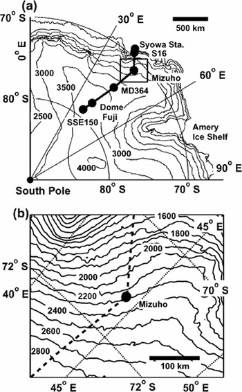
Fig. 1. Elevation map of East Antarctica and the location of Mizuho station (70° 42 S, 44° 17’ E; 2250 m a.s.l, ice thickness about 1950 m). The ice flow is normal to the elevation contours. (a) Solid thick line indicates location of the major 1150 km long traverse route from the summit region of Dome Fuji, through Mizuho station, to Syowa station (Reference Fujita, Matsuoka, Ishida, Matsuoka, Mae and HondohFujita and others, 1999, Reference Gough2002). (b) Elevation contours near Mizuho station and site of the measurements (solid circle).
Fig. 2. Schmidt-net diagram sketches of typical COF development at Mizuho station. (a–c) represent COF in the 700 m deep Mizuho station ice core; (d) is for deeper regions as deduced from the present work. The vertical axis is at the center. Development of vertical-girdle type with increasing depths was observed in the ice core as in (a–c) (see Reference Fujita, Nakawo and MaeFujita and others, 1987). (d) is a typical single-pole COF expected in the simple shear zone deeper in the ice. Stacking of the vertical-girdle-type COF (c) and the single-pole COF (d) is needed to explain the strong radio scattering in the polarization plane along the transverse axis at 900–1500 m depths. This type of COF development was observed in the Vostok deep ice core (Reference Lipenkov, Barkov, Duval and PimientaLipenkov and others, 1989; Reference Lipenkov and BarkovLipenkov and Barkov, 1998).
In 1996/97, we did a more detailed polarization experiment at Mizuho station. Our purpose was to investigate relations between COF within ice and electromagnetic phenomena within ice such as birefringence and scattering. This radar survey was done by the 37th Japanese Antarctic Research Expedition (JARE), which included a series of radar experiments along the 1150km long traverse line from the Dome Fuji region to the coast (Reference Fujita, Kawada and FujiiFujita and others, 1998, Reference Fujita1999,Reference Fujita, Maeno, Furukawa and Matsuoka2002). For these measurements, we varied the following experimental parameters: (1) co-polarization and cross-polarization antenna arrangements; (2) all orientations of the antenna; (3) frequency (60 and 179 MHz); and (4) pulse lengths from 150 to 1000 ns. These results suggested physical conditions of layered stratum in ice and revealed substantial information on how radio-wave scattering responds to these parameters. Moreover, the data suggested that the radio signals were controlled bothby scattering at anisotropic boundaries and by birefringence. We propose that the scattering of radio waves at depths of about 900–1500m is mostly from the stacking of single-pole COF layers with vertical-girdle COF layers. We also suggest that, at depths above about 750 m, the observed anisotropic scattering is likely from the stacking of vertical-girdle-type fabrics with varying cluster strengths. Although our radar experiments are at a single site, the results suggest how similar remote measurements over wider regions can contribute to future understanding of the dynamical structure of the continental ice sheet. We emphasize that much more work should be done to explore the large potential of the polarimetric radar sounding for investigations of the internal structure of polar ice sheets.
Experiment
Basic principle of polarimetric radar sounding
We briefly describe the basic principles used in polarimetric radar soundings. By observing radar signals in two polarization planes and changing the polarization planes of transmitter and receiver with one another, one can obtain more information than from observations with a single fixed polarizationplane. Mostof the convention alradar soundings of polar ice sheets used a single fixed polarization plane. In our polarimetric radar soundings, we rotated the antennas and changed their polarization planes.
Generally, the radar equation describes basic relations between the transmitted signals and the propagation of radio waves in ice including geometrical spreading, attenuation, scattering and refraction, and also includes the specifications of the radar systems. The radar equation used here is described in Reference FujitaFujita and others (1999, Reference Fujita, Maeno, Furukawa and Matsuoka2002) for layered scattering boundaries. However, that equation does not include effects from (1) birefringence and (2) anisotropic scattering boundaries. Therefore, we clarify here how these two phenomena influence the radar power.
Effects from birefringence
Birefringence in ice is often revealed by the transmitting of various colors through ice thin sections between crossed polaroids (e.g. Lang way 1958). In the radio experiments, dipole antennas or Yagi antennas act as imperfect polarizers. These types of antennas transmit and receive radio-wave components mostly in the orientation of the antenna, but side lobes of the antenna radiation pattern produce weak components in various orientations. Therefore, the polarizers are generally less perfect than those for light waves. If the ice sheet has principal axes of birefringence in the horizontal plane, then incident, linearly polarized waves are resolved into two components: the ordinary wave and the extraordinary wave. These two components propagate and scatter separately in ice. Some of the scattered components return to the ice-sheet surface. When these two components appear from the ice sheet to the air, they superimpose into an elliptically polarized wave. A receiver antenna acts as the second polarizer; it detects mostly the electrical field components parallel to the antenna. Depending on the phase difference 0 between the ordinary waves and the extraordinary waves, the waves superimpose either constructively or destructively.
Figure 3 has examples of birefringence for co-polarized and cross-polarized antenna arrangements. For the co-polarized measurement, i.e. when the transmitting antenna Tx is kept parallel to receiving antenna Rx (hereafter denoted as Tx||Rx) and rotated together, a larger power is received when the angle between one of the principal axes and polarization plane is smaller. Thus, maxima and minima of the signal appear alternatively at every integral of 45°. The ratio of the power between the maxima and the minima depends on 0. The average ratio is 3 dB (or 2 on the linear scale). This is the averaged number over both all orientations of the antennas and all phase differences, 0, between the two components. When 0 is close to TT, the ratio can be larger. Therefore, when the observed ratio of the maximum to minimum power is very large, 0 should be close to Ƭ.. However, if the received power is averaged over some depth over a cycle of 0, the birefringence causes the received power to vary by about 3 dB. Also, the signals measured by pulse-modulated radars are essentially interference patterns from many scattering events within a pulse (see, e.g, Reference MooreMoore, 1988; Reference Jacobel and HodgeJacobel and Hodge, 1995). Therefore, the phase of the returned waves should fluctuate significantly.
Fig. 3. Relative variation of the radio-wave power propagated through a uniaxially birefringent ice sheet based on the analysis in Reference HargreavesHargreaves (1977). We assume that the symmetrical axis of birefringence is in the horizontal plane and the vertical-girdle-type fabric of the 700 m Mizuho station ice core. (a) The relative variation of the received power is E2 and the antenna arrangement is Tx||Rx (see text). E2 has the same meaning as in Reference HargreavesHargreaves (1977); E2 means that the received power is the square of the electrical field. E2 is a function of antenna orientation α, defined as the angle of Tx from one of the two principal axes, and 0 is the phase difference between the ordinary and the extraordinary wave. 0 is a function of both anisotropy in the dielectric permittivity tensor in ice and radio frequency. The two principal axes are assumed to be at 0° and 90°. (b) The relative variation of the received power for the Tx ┴ Rx antenna arrangement is E┴2. Antenna orientation α is the angle of Tx from one of the two principal axes. Signals drop when α is along a principal axis.
In cross-polarized measurements, i.e. when the transmitting antenna Tx is kept perpendicular to the receiving antenna Rx (hereafter, Tx ┴ Rx) as both rotate together, the received signal is smallest when the antennas are oriented along the principal axes of the birefringence (Fig. 3b). This is similar to the extinction of light through an ice section between crossed polaroids. Depending on the orientation of the principal axes of birefringence, the polarized electrical field from Tx cannot be transmitted to the orthogonal polarization plane. Therefore, the intensity at Rx is low.
Effects from anisotropic scattering boundaries
If the scattering boundaries within the ice sheet have anisotropic reflectivity with uniaxial symmetry, the received power responds differently to the polarimetric radar sounding (Reference HargreavesHargreaves, 1977). For anisotropic scattering in Tx||Rx measurements, power maxima and minima appear every 90° (Fig. 4a). The ratio between the maximum and minimum power depends on the ratio between the maxima and the minima of the anisotropic reflectivity. For Tx ┴ Rx measurements, the received power is smallest when the antennas are oriented along the principal axes of the anisotropic scattering boundaries (Fig. 4b). Because of the symmetry of the scattering coefficient about the principal axis, the scattered waves along one principal axis do not contribute to the electrical field in the orthogonal plane. Thus, the maximum received signal in Tx ┴ Rx measurements is always smaller than that in Tx||Rx measurements. As indicated in Figure 4b, the ratio between Tx ┴ Rx and Tx||Rx maxima depends on anisotropy in the scattering boundaries, and this ratio will be less distinct in practice because the polarizers are imperfect.
Fig. 4. Relative variation of the received power of radio waves scattered from an isotropic ice sheet containing anisotropic scattering boundaries based on the analysis in Reference HargreavesHargreaves (1977). We assume that the principal axis of the anisotropic reflection coefficient is at orientations of 0° and 90°. We also assume that the amplitude reflection coefficient at 90° is less than that at 0° by a factor of A (A < 1). (a) Antenna arrangement is Tx||Rx. The relative variation of the received power is E||2, which depends on antenna orientation α, defined as the angle of Tx from one of the two principal axes. The variation amplitude of E||2 is |20log10(A)|dB. For example, an A of 0.5 and 0.1 give amplitudes of 6 and 20 dB, respectively. Maxima and minima appear every 90°. (b) Antenna arrangement is Tx ┴ Rx. The relative variation of the received power is E┴2, which depends on α. Antenna orientation α is the angle of Tx from one of the principal axes. Signals drop when α is along a principal axis. The signal strength at the maximum is less than the maximum of E|| 2 by 20 log10 [0.5(1 – A)]dB. For example, when A has values 0.5 and 0.1, the decreases are 12 and 7 dB.
Criteria to distinguish two different effects
In real ice sheets, both birefringence effects and anisotropic scattering boundaries will occur, but the features from the dominant effect will have the clearest influence on the signal. We assume that when both effects occur in the same region of ice, the principal axes of the birefringence equal the principal axes of the anisotropic scattering boundaries. This assumption is justified because both effects are based on the symmetric structure of the COF, and furthermore, this assumption simplifies the problem.
Reference HargreavesHargreaves (1977) originally proposed the following criteria to determine which mechanism is dominating the scattering signal. One first determines the major angles between the maxima and minima in the Tx||Rx measurement. An angle of 90° indicates anisotropic scattering boundaries, whereas an angle of 45° indicates birefringence. If both effects occur, these two variations would be superimposed with common principal axes. In case birefringence dominates, the ratio between the maxima and minima signal would provide 0 as described for Figure 3. When anisotropic scattering boundaries dominate, the ratio between the maxima and minima would provide the magnitude of the anisotropy in scattering boundaries as shown in Figure 4. Whichever effect dominates, one can easily find the principal axes by referring to the signal variations in Figures 3 and 4. By measuring Tx ┴ Rx, one can check to see if the observed phenomenon is from either or both of the two effects. For example, an important feature of the theory of birefringence is that a maximum of one (Tx||Rx or Tx ┴ Rx) component coincides with the minima of the other (that is, Tx ┴ Rx or Tx||Rx, respectively) as shown in Figure 3a and b. Also, an important feature of the theory of anisotropic scattering is that the minimum of the Tx ┴ Rx component coincides with either maxima or minima of the Tx||Rx component (Fig. 4a and b). These features appear in our data.
Radar systems and the method of polarimetric radar sounding
We used a 179 and a 60MHz pulse-modulated radar; the specifications for the transmitters, receivers and recorders for each radar system are given inTable 1.To investigate the effects of radar pulse lengths (i.e. vertical resolution) for the 179MHz radar, we used 150, 350 and 1000 ns. For the 60MHz radar, we used 250 and 1000 ns. Each radar system wasmounted on its own snow vehicle.The radar systemused here was used and calibrated along the 1150 kmtraverse that passed through Mizuho; in this paper, we describe only the Mizuho results.The transmitting antennaTx and the receiving antennaRx were on opposite sides of the vehicle andwere either parallel or perpendicular to each other (Fig. 5). All datawere digitally recorded.To calibrate the received power, we regularly calibrated a relation between the power from the antenna and the output in the recording system during the experiments, which were done from 1996 to 1997 (e.g. Reference Fujita, Matsuoka, Ishida, Matsuoka, Mae and HondohFujita and others,1999, Reference Gough2002).
Fig. 5. Top view of the antenna arrangements. For both arrangements, the transmitting and receiving antennas are at opposite sides of the snow vehicle (rectangle in the figure). Tx and Rx represent transmitting and receiving antennas, respectively. (a) Antenna arrangement for TxkRx measurements. (b) Antenna arrangement for Tx ┴ Rx measurements. The centers of Txand Rx were separated by 6.4 m, and they were 3.2 m above the ice-sheet surface. Antenna lengths were 0.75 and 2.34 m for 179 and 60 MHz, respectively.
Table 1. Specifications of the two radar systems used in this experiment
For Tx‖Rx measurements, we made time series of the radar return power PR in 16 antenna azimuths by changing the direction of the vehicle. For the starting orientation, Tx, Rx and the vehicle were oriented to true north. They were then rotated in clockwise increments of 11.25³ (º/16 rad) until 180³ was reached. Due to symmetry of the radio-wave propagation and scattering around the vertical, orientations 0^180³ are sufficient to describe all angles.We verified this by a number of cross-checks during our experiments.We checked that the results near 0³ and near 180³ were the same at the start of the route, and did the same cross-check at a number of sites along the 1150 km long traverse from Dome F to the coast. Furthermore, at Dome F, the results from 0³ to 180³ agreed very well with the results from 180³ to 360³. In the measurements, orientations were determined using a magnetic compass with errors within a few degrees for each orientation. For Tx ⊥ Rx measurements, the antennas were rotated in the same manner as in the Tx‖Rx measurements.
The detection limit of the present measurements was less than –115 dBm (Table 1). All of the data used here are from –65 to about –115 dBm (e.g. Fig. 6 and 7), which is above the detection limit. Also, we calibrated the system frequently and the total error in the received power is <1dB, so we consider any variation in the time series that exceeds 1dB. But because the signals measured by pulse-modulated radars are essentially interference patterns from many scattering events within a pulse (e.g. Reference MooreMoore, 1988; Reference Jacobel and HodgeJacobel and Hodge, 1995), it is meaningless to discuss each fluctuation of radar signals within a pulse unless discussions are linked with all of the following information on reflectors: (i) exact locations, (ii) distances, (iii) thickness, (iv) types of reflectors (that is, PD, CA or PCOF), (v) orientation of polarization plane, (vi) pulse length, and (vii) radar frequencies. In contrast, one should consider these factors when analyzing the average tendency. We focus on the average tendency in this paper and we do not discuss any single fluctuation.
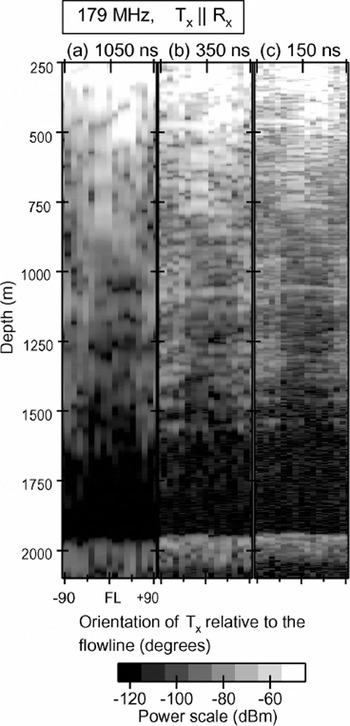
Fig. 6. Radar scattering from ice for the Tx||Rx arrangement at 179 MHz. Abscissa is the Tx orientation relative to the flow-line. The flowline is from 117° to 279° geographically and its orientation is denoted “FL’.’ Ordinate is the depth of ice converted from time data. Received power PR (dBm) is expressed by the gray scale shown at the bottom. Strong signals are white, and weak signals are dark. Images (a–c) are from radar pulse lengths of 1050, 350 and 150 ns, respectively. Received power PR decreases with increasing depth due to geometrical spreading and attenuation of the radio wave. Strong scattering at about 1950 m is from the ice–bedrock boundary. Between 1500 and 1950 m is an echo-free zone due to weak scattering and abrupt drop of received power level at 1500 m (see Reference Fujita, Matsuoka, Ishida, Matsuoka, Mae and HondohFujita and others, 1999, for details). For image (a), PR (dBm) was reduced by 10 dB from the originally observed values so that the same gray scale could be used for all three images.
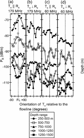
Fig. 7. Variation of PR as a function of antenna orientation for four experimental conditions. PR was averaged over each 250 m from the raw results shown in Figures 6, 8 and 9. Because this averaging distance is much larger than the pulse length in ice (Table 1), the averaged values show signal variations of PR without interference effects. From left to right, the experimental conditions are (a) TxkRx, 179 MHz with 350 ns pulse; (b) Tx ┴ Rx, 179 MHz with 350 ns pulse; (c) TxkRx, 60 MHz with 250 ns pulse; (d) Tx ┴ Rx, 60 MHz with 250 ns pulse. In (a), we fitted the data to sinusoidal curves, except the 750–1000 m data. The error caused by the interference effect is about ±1dB.
Glaciological conditions of the observation site
The ice sheet near Mizuho station is in the Shirase Glacier drainage basin, where ice flow converges toward the outlet glacier (Fig. 1b). The flow vector of the ice sheet is 22.2 m a–1 in the direction of 297°(Reference MotoyamaMotoyama and others, 1995). The principal strain was derived as tensile in the longitudinal direction and compression in the transverse direction (Reference Naruse and ShimizuNaruse and Shimizu, 1978). At Mizuho station, Reference Yoshida, Yamashita and MaeYoshida and others (1987) did experiments at a point 0.2 km west of the main buildings of the station. Our new experiment was done at a point 0.2 km east of the main buildings of the station to avoid possible interference between our radar experiment and facilities of the station. Therefore, the distance between two sites is 0.4 km. At the station, a 700 m long core was drilled in 1983 and 1985 (Reference A., Nakawo, Narita, Fujii, Nishio and WatanabeHigashi and others, 1988). The COFs of the 700 m long core are vertical-girdle type due to tensile strain, and this type develops with increasing depth (Reference Fujita, Nakawo and MaeFujita and others, 1987).
Results
Response of received power PR to polarimetric radar sounding at 179 MHz
The Tx||Rx measurements at 179 MHz show that the dependence of PR on antenna orientation is different for depths above and below -750 m (Fig. 6). At depths above about 750 m, PR is strongest for antenna orientations near the flow-line and weakest for antenna orientations perpendicular to the flowline. Here, the orientation is expressed as an angle relative to the flowline. Hereafter, we denote an orientation perpendicular to the ice flow as “transverse”. Because the angle between the maxima and minima is 90°, anisotropic scattering boundaries have strong effects. This feature was found to be independent of pulse length and thus is unlikely to be caused by interference within a pulse. Although the pulse-modulated radar signals are essentially interference patterns from multiple scatterings within a pulse, we confirmed that changes of vertical resolution (i.e. pulse lengths) did not affect the general trends in PR. On the other hand, small fluctuations of the order of several dB over depth ranges as narrow as the pulse lengths (see Table 1) indicate interference effects. But, the average trends over significant depths are clear. To better illustrate the variation trends with depth, the raw PR data were averaged over each 250 m (Fig. 7a). At depths of 250–500m, the variation amplitude is about 10 dB. At depths of 500–750 m, the variation amplitude is about 8 dB. At depths of 750–1000m, the variation is smallest.
An interesting feature is that the orientations of maxima and minima are opposite at depths below about 900 m as compared with regions closer to the surface (Fig. 6 and 7a). That is, below about 900 m, the maxima appear along the transverse line, whereas the minima appear along the flowline. This feature appears in the three images of Figure 6 and in Figure 7a. The variation amplitude is about 10 dB at depths below about 900 m. Although the maxima and the minima switch between shallow and deep regions, the principal axes have the same orientations; in both cases, they are along the flowline and the transverse line.
The Tx ┴ Rx measurements at 179 MHz showed features in agreement with theory. Figures 7b and 8 show clear variations of PR with antenna orientations. At most depths where the signal is above the detection limit, the PR signals are strong at about 45° from the principal axes on both sides, as theory predicts in Figure 4. Also, minima appear mostly at the two principal axes, which also agrees with Figure 4. As in the Tx||Rx measurements, little variation occurs between about 750 and 1000 m. As in the previous figure, these features are common to the three pulse lengths and thus are unlikely to be interference effects.

All of the features in the Tx||Rx measurements are consistent with earlier Tx||Rx observations at Mizuho. For example, Reference Yoshida, Yamashita and MaeYoshida and others (1987, fig. 5) and Reference Fujita, Mae and MatsuokaFujita and Mae (1993, fig 2) pointed out that both the 90° angle between the maxima and minima, and the maxima and minima switch between shallow and deep regions. This agreement shows the consistency and reliability of the measurements.
Response of received power PR to polarimetric radar sounding at 60 MHz
The orientation dependence of PR is weaker at the lower frequency of 60 MHz. For example, the gray-scale images for Tx||Rx in Figure 9a and b do not show a very clear trend of PR with orientation. However, peaks at the flowline and the transverse line clearly appear when the signals are averaged over each 250 m (Fig. 7c). The angles between maxima and minima are near 45° at most depths. According to the theory, this is a typical feature of birefringence. As with the 179 MHz data, the variation is much weaker at 750–1000 m.
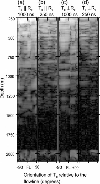
Fig. 9. TxkRx and Tx ┴ Rx measurements at 60MHz. Otherwise, features and gray scale are the same as in Figures and 8. Two pulse lengths, 1000 and 250 ns, were used. From to right, the antenna arrangement and pulse lengths for image are (a) TxkRx and 1000 ns, (b) TxkRx and 250 ns, (c) Tx ┴ Rx and 1000 ns, and (d) Tx ┴ Rx and 250 ns.
An interesting feature is that, at depths below 750 m, the PR signals for the 60 MHz Tx||Rx measurement have features in common with those of the 179 MHz measurements (cf. Fig. 7a and c). Although the 60 MHz data in Figure 7c have additional maxima, the large maxima are common to the 179 MHz data in Figure 7a. Such comparisons between frequencies have important implications for the operation of a common scattering mechanism in ice, as discussed in the next section.
The gray-scale images for Tx ┴ Rx in Figure 9 show clear variations of PR with antenna orientations (Fig. 9c and d). At most depths where the signal is above the detection limit, PR signals tend to be strong at two orientations, about 45° away from the flowline and transverse line, whereas minima occur near the flowline and near the transverse line. These features are common to both pulse lengths, indicating that they are not interference artifacts. Furthermore, except at 250–500m and 750–1000m, the averaged data show clear variations (Fig. 7d).
In addition to the 45° angles between maxima and minima in the Tx||Rx measurement, the data agree with birefringence theory (Fig. 3) in another way. Theory predicts that a maximum of one (Tx||Rx or Tx ┴ Rx) component coincides with the minima of the other (that is, Tx ┴ Rx or Tx||Rx, respectively). Figure 7c and d agree with this prediction at most depths where the signal showed clear variations.
Discussion and Interpretation
Many observed features agreed well with theories of either (1) birefringence, (2) anisotropic scattering boundaries, or both. We first discuss how birefringence and anisotropic scattering boundaries occur in the ice sheet. In particular, we focus on the causes of radio-wave scattering in the ice sheet and its dependence on frequency. Second, we suggest that COF varies with depth at Mizuho. Third, we discuss abrupt changes of COFs in the Antarctic ice sheet. Finally, we describe how the method can be extended to measurements over wide areas.
Causes of radio-wave polarization and scattering and their response to frequencies
Interpretation for the 179 MHz data
The Tx||Rx measurements at 179 MHz strongly suggest features of anisotropic scattering boundaries because the angles between maxima and minima are about 90°. The features agree well with those from the earlier Tx||Rx experiments at Mizuho reported by Reference Yoshida, Yamashita and MaeYoshida and others (1987), Reference Fujita, Mae and MatsuokaFujita and Mae (1993) and Maeno and others (1995). Macroscopic dielectric permittivity tensor data from the ice core also suggest birefringence (Reference Fujita, Mae and MatsuokaFujita and Mae, 1993). Neither the earlier nor the present data rule out the birefringence effect. This is because a large PR appears in one of the two anticipated principal axes. This fact suggests that birefringence effects occur, but the signal is the weakest in one of the principal axes due to weak reflectivity in that orientation. In other words, birefringence alone cannot explain the major angle between the maxima and the minima, because anisotropic scattering boundaries are needed to explain this observation. We therefore conclude that, for the 179 MHz radio wave, scattering boundaries have anisotropy as large as 10 dB on the power decibel scale. Considering the imperfect polarizing of the radio antennas, the real anisotropy should be larger. The principal axes are along the flowline and the transverse line. In addition, the orientations of the PR minimainthe Tx ┴ Rx measurements agree with theory (Fig.4b). Because the evidence suggests that birefringence and anisotropic scattering boundaries have the same principal axes, orientations of the PR minima in Tx ┴ Rx measurements do not contradict the birefringence theory. The features of the maxima and minima in Figure 7b are consistent with theories of both birefringence in Figure 3b and the anisotropic scattering boundaries in Figure 4b.
According to a two-frequency radar experiment at Mizuho, the dominant cause of radio-wave scattering is changes in permittivity and not changes in conductivity at all depths (Reference FujitaFujita and others, 1999). According to this constraint, radio-wave scattering can be caused by PD and PCOF at 179 MHz. CA scattering should not be a dominant mechanism at Mizuho at179 MHz. Reference FujitaFujita and others (1999) also argued that the dominant cause of radio-wave scattering is PCOF at least at depths below about 700–900m. This is because the hydrostatic pressure and the transformation of air bubbles into clathrate hydrate crystals should reduce density fluctuations deep in the ice sheet. But the PD/PCOF boundary might be shallower if densification occurs more rapidly and if shearing is stronger at Mizuho. This is possible because Mizuho is located in a warmer and steeper region than dome summit regions (Fig.1a). We also note that clathrate hydrate crystals cannot have any significant effect on the dielectric permittivity, due to its very small volume fraction, of the order of 3610–4 (e.g. Reference Lipenkov and HondohLipenkov, 2000).
In addition to supporting previous findings, this study finds (i) at depths below about 900 m, the scattering is strongest along the transverse line; and (ii) at depths above about 750 m, the scattering is strongest along the flowline. We suggest that 6 PCOF is the only possible cause of the strong anisotropic left scattering at depths below about 900 m. CA is ruled out based each on results from the two-frequency experiments, and although PD might cause anisotropic scattering, the depths are too great to allow any PD mechanism to occur. Moreover, COF changes within a horizontal plane would naturally cause very strong anisotropy in the scattering boundaries. Figure 2a–c are sketches of three typical examples of COF at Mizuho. If the COF changes from one to another within a short distance, the scattering boundaries would become essentially those of an anisotropic tensor. Indeed, such changes of COF occur in Vostok deep ice (Reference Lipenkov and BarkovLipenkov and Barkov, 1998). We do not have ice-core COF data from 700 m to the base of the ice sheet at about 2000 m; however, the vertical-girdle-type COF due to tensile strain, discovered in the shallower region of the Vostok deep ice core (Reference Lipenkov, Barkov, Duval and PimientaLipenkov and others, 1989), would be an important reference to deduce how the COF at Mizuho develops in deep regions. Indeed, COF of the 700m Mizuho station core and COF of the shallow side of Vostok station core are very similar. Also, interpretations of the data are qualitatively the same (cf. Reference Fujita and MaeFujita and others, 1987; Reference Lipenkov, Barkov, Duval and PimientaLipenkov and others, 1989). Lipenkov and Barkov (1998) reported that, as they investigated deeper, there were two types of COFs, vertical-girdle and single-pole. Moreover, they discovered a layered ice stratum composed of these two types of COFs. Their work is important evidence for COF in deep regions at Mizuho and also evidence of sharp changes of COFs in deep polar ice. We discuss this in detail further below. Thus, the facts that
-
(i) variations are due to permittivity changes,
-
(ii) depths are too great to allow any PD mechanism to occur,
-
(iii) strongly anisotropic reflection boundaries are explained by the PCOF mechanism, and
-
(iv) layered strata composed of different COFs are known to exist
lead us to suggest that the major cause of the 179 MHz radio scattering at depths below about 900 m at Mizuho is PCOF.
The situation above about 750 m is different for several reasons. First, fact (ii) does not apply. Second, fact (iii) might apply, but if the PD mechanism also causes some anisotropy, (iii) cannot apply only to PCOF. In fact, it is well known that the depositional environment in Antarctica is highly anisotropic due to the prevailing wind, causing large sastrugi and dunes. Such depositional features might cause unknown anisotropic effects in the radio-wave scattering due to the PD mechanism. For condition (iv), there seems to be no study that investigated fluctuations of the vertical-girdle-type COF on scales of millimeters to several meters. Therefore, our knowledge on the shallower scattering is that permittivity-based reflections have strong anisotropic features at Mizuho. We need more information to determine the relative contributions from PD and PCOF mechanisms. To examine whether or not the PD mechanism can cause anisotropic scattering boundaries due to a depositional environment related to sastrugi and dunes, one should examine the echoes from 250 m andabove. This is because the shallowest echoes would likely come from density fluctuations, so one can check directly if echoes from the PD zone have effects from anisotropic boundaries. Echoes from other mechanisms would be weaker. Indeed, Reference Nakawo and NaritaNakawo and Narita (1985) measured the density profile of the Mizuho station ice core. Above about 250 m, density fluctuations were up to about 1kgm–3. This fluctuation can produce a power reflection coefficient as large as about –50 dB. The power reflection coefficient from PCOF and CA is generally well below–60 dB (Reference Fujita, Matsuoka, Ishida, Matsuoka, Mae and HondohFujita and Mae, 1994; Reference Fujita, Matsuoka, Ishida, Matsuoka, Mae and HondohFujita and others, 2000). Figure 10 gives variation of PR averaged over 70 m thick regions from depths of 180–250m, our shallowest data. The averaged PR is shown as a function of antenna orientation for Tx||Rx and Tx ┴ Rx at 179 MHz. We emphasize here that signal variations are consistent with birefringence theory (Fig. 3) and no features suggest anisotropic scattering boundaries. Therefore, the data from the shallow PD zone did not show effects from anisotropic depositional features. This fact suggests that the PCOF mechanism caused the strong scattering when the polarization plane was along the flowline at 179 MHz. This fact also suggests that there is a boundary between the shallow PD zone and the PCOF zone at depths somewhere around 250 m at Mizuho.
Fig. 10. Variation of PR as a function of antenna orientation for 70 m thick depths between 180 and 250 m. Frequency pulse length are 179 MHz and 350 ns, respectively. Results from Tx||Rx measurement and Tx ┴ Rx measurement are given as solid circles and open circles, respectively. PR was averaged over 70 m from the raw results. The error estimates are for the fluctuations due to the interference effect.
Relative and contribution of the birefringence and the anisotropic scattering boindary
The Tx||Rx measurements at 60 MHz showed stronger features of birefringence, that is, the angle between the PR maxima and minima is 45° at most depth ranges, which is similar to the birefringence example in Figure 3. Also, the results do not have strong indications of anisotropic scattering boundaries (e.g. the superimposed 90° component of angles between the large PR and small PR is weak except near 1000–1250 m). The principal axes of birefringence are close to the flowline and the transverse line as before. The minima of the Tx ┴ Rx measurements are also consistent with Figures 3b and 4b.
The 60 MHz data cannot be explained solely by birefringence, nor solely by anisotropic scattering. This is because, at depths of around 1000–1250 m, the PR signals for Tx||Rx still have a strong feature typical of anisotropic scattering boundaries. Indeed, in Figure 7c, the difference in PR maxima between the two principal axes is about 4– 5dB. This feature cannot be explained by birefringence alone. Also, at depths of around 500–750 m, the PR signals for Tx||Rx still have large maxima at the flowline like those at 179 MHz. Therefore, both effects are necessary to explain the observed data at 60 MHz even though the scattering boundaries are less anisotropic than those at 179 MHz.
To determine how PD, CA and PCOF contribute to scattering at 60 MHz, we focus on the relative contributions from birefringence and anisotropic scattering boundaries. An observational fact is that birefringence apparently contributed to scattering at 60 MHz but not at 179 MHz. We suggest that the CA mechanism caused the dominant radio scattering at 60 MHz. The CA mechanism is stronger at lower frequencies (Reference MooreMoore, 1988; Reference Fujita, Nakawo and MaeFujita and Mae, 1994; Reference FujitaFujita and others, 1999,Reference Fujita, Matsuoka, Ishida, Matsuoka, Mae and Hondoh2000), whereas both PD and PCOF mechanisms are independent of frequency. In addition, radio scattering caused by the CA mechanism is largely isotropic; data have not shown strong anisotropy in the electrical conductivity of ice in the MHz range. In contrast, radio scattering caused by the PCOF mechanism is largely anisotropic.
In summary, at Mizuho at 179 MHz, the PCOF mechanism dominates below about 250 m, causing a strong anisotropy in reflectivity. At depths shallower than about 250 m, the PD mechanism dominates. At 60 MHz, the contributions of CA and PCOF are roughly equal. Therefore, the scattering boundaries are less anisotropic and effects from birefringence clearly appear. But PCOF gave stronger effects at depths near 1000–1250m. According to the two-frequency radar sounding along the traverse route, ice at depths near 1000–1250 m at Mizuho is a high shear zone that strongly illuminates the incident radio wave(see Reference Fujita, Matsuoka, Ishida, Matsuoka, Mae and HondohFujita and others, 1999, plate 2e). The data here suggest that the strongest anisotropy due to PCOF occurs in the high shear zone where the CA mechanism cannot dominate, even at 60 MHz.
Variation of COF with depth
Crystal-orientation fabrics above 750 m
Our primary motivation here is to extract information about COF using the polarimetric radar sounding and to use the COF information to better understand the physical conditions in ice, particularly the ice-flow regime. We first infer the COF according to the strong scattering in the flowline orientation at depths more than about 750 m. In the shallower ice, the 700m Mizuho station ice core has the COF sketched in Figure 2a–c. The c axes of the grains gradually concentrated on a vertical girdle with increasing depth. It is important to determine why strong scattering at 179 MHz occurred only when the polarization plane was oriented along the flowline. A plausible explanation is that the cluster strength of the vertical-girdle fabric changes from one depth to another. In this case, major changes in the macroscopic dielectric permittivity tensor appear mainly along the symmetrical axis of the uniaxial tensor, that is, along the flow-line. Viewed from the symmetrical axis, the development of a vertical-girdle-type fabric means that all of the caxes move away from the symmetrical axis. The other two axes, the vertical axis and the transverse axis, are almost equivalent. Along each of these two axes, the macroscopic dielectric permittivity is always as large as that of a random fabric. Therefore, we deduce that the development of the vertical-girdle type significantly changes the dielectric permittivity tensor along the flowline axis, but it has little effect on the other two axes. No study has yet investigated fluctuations of vertical-girdle-type COF over scales of several millimeters to meters. We clearly need verification from ice cores like Mizuho or Vostok to better understand the mechanism that causes fluctuations of the vertical-girdle-type COF.
Crystal-orientation fabrics at 750–900 m
The stacking structure of COF at depths below about 750– 900 m should be different from the upper vertical-girdle type. This is because the maxima of PR in the TxkRx measurements are not clear. Also, at 700 m, the COF already has a well-developed, vertical-girdle-type fabric in the ice core (Reference Fujita, Nakawo and MaeFujita and others, 1987). Thus, the vertical-girdle-type fabric cannot continue to develop because the crystal grains cannot rotate, even with greater tensile strain. Under such a well-developed vertical-girdle-type fabric, the deformation mechanism of ice is not basal glide motion of crystal dislocations. Instead, non-basal glide motion of dislocations, climb motion (Reference Hondoh and HondohHondoh, 2000) and possibly recrystallization are necessary to cause further tensile strains. Moreover, Reference AzumaAzuma’s (1994) anisotropic flow law predicts that the strain rate of a well-developed vertical-girdle-type fabric is about 10 times smaller than that of isotropic ice. Therefore, ice with a well-developed vertical-girdle-type fabric is hard ice in which the orientation of each c axis cannot change, even with greater tensile strain. The disappearance of anisotropy in the scattering boundaries between 750 and 900m (Fig. 9a) was likely caused by this saturation of basal-plane-motion-based tensile strain in ice. Thus, there should be well-developed, vertical-girdle-type fabrics at depths of 750–900m.
Crystal-orientation fabrics below about 900 m
Below about 900 m, the maxima of PR in the TxkRx measurements appear when the polarization planes are oriented in the transverse line. Thus, there should be changes of the dielectric permittivity tensor component in this axis. Thever-tical-girdletype alone cannot explain changes of the tensor in this orientation. Traverse radar measurements (antennas oriented only along the traverse line) near Mizuho station showed that the radio waves scattered strongly at these depths (Reference Fujita, Matsuoka, Ishida, Matsuoka, Mae and HondohFujita and others, 1999). Considering that deeper ice generally has high shearing and that high shearing of ice produces a single-pole crystal fabric, layers with a single pole should occur. However, single-pole fabrics alone cannot cause anisotropic scattering because single poles have an isotropic dielectric permittivity tensor in the horizontal plane.
A basic property of the single-pole fabric under high shearing in the ice sheet is that initial small fluctuations of viscosity along depths are amplified by positive feedback into regions of highly strained ice and regions with little strain. That is, deformed ice becomes softer and deforms more readily, thus forming a stronger single-pole fabric than the surrounding ice (see, e.g., Reference PatersonPaterson, 1991; Reference Lipenkov and BarkovLipenkov and Barkov, 1998). Because strains in ice respond highly non-linearly to given stresses (e.g. the non-linearity in flow laws), this amplification should be strong. When high shear zones have such strong amplification, a strong single-pole fabric appears in several limited depth ranges (further details are in section 4.1.3 of Reference Fujita, Matsuoka, Ishida, Matsuoka, Mae and HondohFujita and others, 1999). Several real examples including the high shear zones in deep regions of Vostok ice cores are discussed below. Considering this suggested basic nature of COF development, we suggest that only one scenario can explain all of the observational facts obtained in this study. As in the high shear zones of Vostok deep ice cores, ice is a layered ice stratum composed of both well-developed, vertical-girdle-type fabric as in Figure 2c, and single-pole fabric as in Figure 2d. Layers of single-pole COF have greater response to shear stress, whereas layers of vertical-girdle-type COF have greater response to stress from convergent ice flow than to shear stress. In this case, radio waves will scatter strongly only in the polarization plane of the transverse direction because the contrast between Figure 2c and d gives a contrast of the dielectric permittivity tensor only in the transverse direction. Such a contrast causes scattering anisotropy well above 10 dB. It also gives a scattering coefficient as large as –60 dB in power in orientations of maximum reflectivity (Reference Fujita and MaeFujita and Mae, 1994; Reference Fujita, Matsuoka, Ishida, Matsuoka, Mae and HondohFujita and others, 2000). This value is extremely large as the scattering coefficient at the deeper side in polar ice sheets. We therefore suggest that, below about 900 m to the deepest limit of the PCOF zone at about 1500 m, the ice has layers of vertical-girdle-type fabric stacked amongst layers of single-pole fabric.
Abrupt changes of COFs in the Antarctic ice sheet
Four examples
Because there is some debate about whether or not COF changes can occur over scales short enough to cause radar scattering, we describe below four reports of rapid COF changes in Antarctic ice.
The most common COF at Vostok is the vertical-girdle type associated with relatively coarse-grained interglacial ice, although single-pole fabric occurred in fine-grained glacial ice (Reference Lipenkov and BarkovLipenkov and Barkov, 1998). Reference Lipenkov and BarkovLipenkov and Barkov (1998) report that the difference between these two COFs is very small in the upper section of the ice sheet but increases with depth and is very clear below 2700 m. Moreover, they found a layered ice stratum composed of these two types of COF at 3460–3538m. The thickness of the single-pole COF layers enclosed by vertical-girdle COF layers was of the order of several millimeters to several centimeters (Reference Duval, Lipenkov, Barkov and S.Duval and others, 1998; personal communication from V. Ya. Lipenkov, 2002). This indicates that ice sheets characterized by vertical-girdle-type COF can have a stacking structure when subjected to high shearing deep in the ice.
Abrupt changes of COFs were also found in an ice core drilled at Dome F, a region without flow. Reference Azuma and T.Azuma and others (2000) discovered that the cluster strength of the c axis around the vertical changed in many layers within the last glacial age (500–800m) in the Dome F Antarctic ice core. In addition, N. Azuma (personal communication, 1999) used the newly invented automatic ice-fabric analyzer (Reference Yun and AzumaWang and Reference AzumaAzuma, 1999) and found that the ice contains significant fluctuations of cluster strength, even in 1 m long cores. The “medianinclination” (defined by Reference Azuma and T.Azuma and others, 2000) changed by as much as 10° within a distance of several centimeters.
Reference Gow and WilliamsonGow and Williamson (1976) investigated the COF in a Byrd Station ice core and described six cloudy bands that contain visible volcanic-glass shards. Below 910 m, the COF was more tightly clustered about the vertical in the cloudy bands than in the enclosing ice. The bands were 1–60 mm thick. Because the crystal sizes of such layers were always much smaller than those of the enclosing ice and had a fragmented appearance, they argued that such layers might constitute zones of actual shear displacement in the ice sheet. This is a valid example of sharp COF change, although COF changes in our data may be different from this example.
The last example is the study by Reference Thwaites, Wilson and MccrayThwaites and others (1984). They investigated the relationship between borehole closure rate and COF in the ice cores from Cape Folger, Antarctica. Cape Folger is near the coastal margin of the ice sheet at Law Dome. The closure rate was highly dependent on depth and was closely related to the COF of the ice. The zones at which the non-uniform closure occurred were 0.5–3 m wide. This suggests that the COFs changed over scales of 0.5–3 m .
The above four examples indicate that there are significant COF fluctuations under at least four conditions: (i) the dome summit at Dome F; (ii) flowing ice at Vostok, 250 km from an ice divide (ridge B); (iii) cloudy bands and enclosing ice in the Byrd Station ice; and (iv) Cape Folger ice near the coast. Until recently, measuring COF changes over sub-meter distances on deep ice cores has been too time-consuming, and thus, Reference Yun and Azumaexcept for the above examples, direct evidence for abrupt COF changes remains weak. But with the new methods pioneered by Wang and Reference AzumaAzuma (1999) and the indirect indications of abrupt COF changes in this study, this debate over abrupt COF changes should be resolved soon. The four examples given here are all for different conditions; thus, abrupt changes of COFs might be widespread in Antarctic ice. Open question: mechanism causing the abrupt changes Two examples of abrupt COF changes, that at Dome F and that deduced at Mizuho atdepths above about 750 m, cannot be explained by positive feedback between softening of the strained ice and simple shear strain. This is because stress– strain configuration at Dome F is not simple shear. It is more likely uniaxial compression or pure shear typical for a dome region and ice-divide zones. At Mizuho, the stress–strain configuration is uniaxial tension. In all three types of stress– strain configurations (uniaxial compression, pure shear and uniaxial tension), strain hardens the ice except for the initial 10–30%of the strain that softens ice (see anisotropic flow law and Azuma, 1994, fig. 5). At Dome F, the vertical compression is well above 10–30%. Also, according to the strain-history analysis of a Mizuho station ice core (Fujita and others, 1987, fig. 7), the total tensile strain is 40–140% at about 100–700m. Therefore the initial strain softening cannot be a major reason for the contrasts of COFs in uniaxial strain. These facts imply an important feature of ice textures in polar ice sheets. That is, abrupt changes in simple shear are only a secondary, yet important, effect of ice flow. Before ice reaches depths at which it is subjected to simple shear, there is already some primary mechanism that produces initial abrupt COF changes. The primary mechanism seems to be related to several properties in ice, such as changes of impurity content typical for glacial-age/interglacial-age ice, grain-size and shape, or initial depositional environment (e.g. Reference PatersonPaterson, 1991; Reference Lipenkov and BarkovLipenkov and Barkov, 1998; Reference Azuma and T.Azuma and others, 2000). Based on our discussion of the shallow side of Mizuho, together with the observation for the Dome F ice, relations among these shouldbe extensively investigated to understand the primary cause of COF changes.
Concluding Remarks
Based on our polarimetric radar experiments at Mizuho station, we suggest the following conclusions:
-
(1) At 179 MHz, radar signals are strongly controlled by anisotropic scattering boundaries with anisotropy as large as 10 dB.
-
(2) At 179 MHz, the major cause of the radio scattering below about 250 m at Mizuho is PCOF.
-
(3) At 60 MHz, the major causes of radio scattering at Mizuho are PCOF and CA. However, at high-shear zones, PCOF has the stronger influence.
-
(4) Between 250 and 750 m, it is highly likely that the ice sheet has stacking of the vertical-girdle-type fabric with various cluster strengths. Between 750 and 900m, there is a zone of well-developed, vertical-girdle-type fabric.
-
(5) Below about 900 m and until the deepest limit of the PCOF zone, the ice has layers of vertical-girdle-type fabric stacked amongst layers of single-pole fabric as found previously in a Vostok deep ice core.
These conclusions and suggestions should significantly influence the understanding of ice dynamics and radar-sounding techniques on ice sheets. However, important questions remain: (a) Why is this ice sheet composed of such a stacking structure, and how widespread are the structures? (b) How does such a stacking structure affect our understanding of ice dynamics, and how might it lead to better modeling? (c) What is the origin of the COF fluctuations, and how do they develop during ice flow from the dome summit to the coast? (d) Why does the fabric strength vary/jump with depth in stress–strain configurations of uniaxial compression, pure shear, uniaxial tension, and without simple shear? To answer these questions, additional radar data are required, particularly from traverses along the ice flow and its transverse direction. We suggest that radar is, presently, the only way to investigate COF over wide regions in polar ice sheets. The experiments here are from a single site, but similar radar measurements over wider regions might provide invaluable information on the physical structure of polar ice sheets. We hope that the recent polarimetric radar sounding along several traverse routes by the 40th Japanese Antarctic Research Expedition (JARE) in 1999/2000 (Reference Matsuoka, Maeno, Uratsuka, Fujita, Furukawa and WatanabeMatsuoka and others, 2002) will provide some of the answers. Also, we expect that automatic fabric analyzers will provide many more datasets of continuous COF measurements along ice cores. By combining the radar data with ice-core data, we should be able to better understand the three-dimensional dynamical structure of polar ice sheets.
Acknowledgements
This paper is a contribution to the Dome Fuji Project, a program conducted by the Japanese Antarctic Research Expedition. We thank the science editor, T. Thorsteinsson, and three anonymous reviewers for their kind and critical review and for their efforts to improve the paper.


