


1. Introduction
Flexibility is a relevant feature of the flapping appendages of natural fliers and swimmers, which can lead to greatly improved propulsive performance. This enhancement of the propulsive capabilities of flexible flapping foils has been analysed and explained in a large number of works, especially for the simplest configuration of a two-dimensional flapping foil with chordwise flexibility, as in the pioneering experimental works of Heathcote, Martin & Gursul (Reference Heathcote, Martin and Gursul2004) and Heathcote & Gursul (Reference Heathcote and Gursul2007) (see, for example, Wu (Reference Wu2011), Wang & Zhang (Reference Wang and Zhang2016) and Smits (Reference Smits2019) for comprehensive reviews). To the large number of dimensionless parameters characterizing the kinematics of flapping rigid foils, flexibility, and in general the fluid–structure interaction, adds some new ones such as the dimensionless stiffness  $S$, or ratio of elastic to fluid forces, and the mass ratio $R$, or ratio of solid to fluid inertia, in addition to a number of geometric parameters characterizing the deformation of the foil. Therefore, the analysis of the propulsive performance of flexible foils becomes cumbersome, even for two-dimensional foils and once the numerical or experimental difficulties associated with solving or measuring the fluid–structure interaction have been circumvented, since many simulations or measurements have to be made to cover the influence of all the parameters on the propulsive performance (see, for example, Quinn, Lauder & Smits (Reference Quinn, Lauder and Smits2015) and Olivier & Dumas (Reference Olivier and Dumas2016) for representative experimental and numerical studies, respectively). Thus, to dispose of analytical solutions characterizing the fluid–structure interaction of flexible flapping foils, even for very simplified configurations, is very helpful, both to understand the propulsive performance of flying and swimming animals and to design and improve bio-inspired flying and swimming robotic models. These analytical approximations have to be searched within the framework of the two-dimensional linearized inviscid flow theory for small deformations of the foil, pioneered by Wu (Reference Wu1961), who considered a flapping plate that incorporated flexibility, allowing it to deform according to the fluid and elastic forces it experiences. Passive flexibility changes the thrust that a flapping plate generates, and consequently its propulsive efficiency. Particularly, compared with rigid foils, it has generally been found from these inviscid flow theories that flexibility produces greater thrust when actuated near a fluid–structure natural frequency, but less otherwise, with propulsive efficiency greater than that of a rigid foil over a broad range of frequencies and stiffnesses (Katz & Weihs Reference Katz and Weihs1978; Alben Reference Alben2008; Michelin & Llewellyn Smith Reference Michelin and Llewellyn Smith2009; Alben et al. Reference Alben, Witt, Baker, Anderson and Lauder2012; Floryan & Rowley Reference Floryan and Rowley2018, Reference Floryan and Rowley2020).
An interesting analytical approach, within the linear inviscid limit considered in the present work, was recently presented by Moore (Reference Moore2014), who considered the particular case of a rigid foil with a prescribed heaving displacement and a passive pitching motion about its leading edge, relating the finite torsional stiffness of the leading edge with the kinematics of the rigid pitching motion and, hence, with the propulsive performance of the foil. More general approaches based on Wu's inviscid theory (Wu Reference Wu1961) and the Euler–Bernoulli beam equation for small amplitudes have appeared recently, where the displacement of the foil and the fluid motion are decomposed into a Chebyshev series with a large number (infinite in theory) of parameters that have to be obtained numerically (Alben Reference Alben2008; Moore Reference Moore2017; Floryan & Rowley Reference Floryan and Rowley2018; Tzezana & Breuer Reference Tzezana and Breuer2019; Floryan & Rowley Reference Floryan and Rowley2020). All these works considered heaving and/or pitching motions about the leading edge of the foil and computed the thrust force from the projection of the pressure force into the flight direction plus the leading-edge suction (Garrick Reference Garrick1936; Wu Reference Wu1961, Reference Wu1971). Here, however, we follow a simpler approach that provides analytical results by just considering a quartic deflection of small amplitude superimposed on the heaving and pitching motions of the foil, now about any pivot point location along the foil, not just the leading edge. Technically, the approach may be considered as a low-order expansion, or minimal model of a flexible foil. For this kinematics with low-amplitude flexural motion, which structurally is valid when the stiffness of the foil is sufficiently large, we use analytical results derived very recently for the propulsive performance of a pitching and heaving foil with a small flexural deflection (Alaminos-Quesada & Fernandez-Feria Reference Alaminos-Quesada and Fernandez-Feria2020), computing the thrust force from a general vortical impulse formulation (Fernandez-Feria Reference Fernandez-Feria2016). These kinematic-based results are coupled with the dynamics of the foil through the Euler–Bernoulli beam equation to compute the amplitude  $d_m$ and the phase shift $\psi$ of the flexural deflection in terms of $R$,
$R$,  $S$ and the kinematic parameters of the prescribed heaving and pitching motions about any given pivot point. The thrust, lift and moment exerted by the fluid on the foil are then obtained using the analytic general results for prescribed kinematics and deformation based on the impulse formulation (Alaminos-Quesada & Fernandez-Feria Reference Alaminos-Quesada and Fernandez-Feria2020). Thus, the present paper puts in a proper dynamical context the results in Alaminos-Quesada & Fernandez-Feria (Reference Alaminos-Quesada and Fernandez-Feria2020), which considered just the kinematic problem, i.e. these former results provided the propulsion performance of a flapping foil when not only the heaving and pitching components of the motion were prescribed (forced), but also its flexural deformation as a quadratic deflection. Here this flexural deflection, now as a quartic polynomial approximation, is obtained from the dynamics of the foil in terms of its structural properties (stiffness, density, thickness, etc.) through the beam bending equation, for any given heaving and pitching motion applied at an arbitrary pivot point. Thus, the effect of flexibility on the propulsion performance of the foil is finally obtained in terms of the dimensionless stiffness and mass ratio of the foil, in addition to all the kinematic parameters.
In the approximation presented in the present work, the input power is obtained directly from the dynamic beam equation in terms of the input force and torque exerted externally on the pivot point, plus the effect of the inertia of the foil through the mass ratio  $R$. The results are valid for a wide range of mass ratios, covering the typical values of both flapping swimming and flapping flight with flexible foils.
The paper is organized as follows. The formulation of the problem, including the general moments of the Euler–Bernoulli equation relating the input force and torque with the lift, moment and flexural coefficients, is given in § 2 together with the kinematics of the foil and the corresponding analytical expressions for the above-mentioned coefficients. Section 3 presents the analytical expressions for the first natural frequency of the system, as well as the amplitude and phase shift of the passive flexural deformation, and the corresponding thrust coefficient, input power coefficient and propulsive efficiency. These expressions are used in § 4 to characterize the propulsive performance of heaving and pitching foils about any pivot point in terms of the forcing frequency, stiffness and mass ratio of the foil, with more detail for a purely heaving motion forced on any pivot point, not just the leading edge as in most previous works. Finally, the conclusions are presented in § 5.
2. Formulation of the problem
We consider a two-dimensional foil of chord length  $c$ immersed in an incompressible and nearly inviscid flow with constant free-stream speed $U$ along the $x$ axis. We use non-dimensional variables scaled with the half-chord length $c/2$ and the velocity $U$. A harmonic heaving motion along the $z$ axis, $h(t)$, is imposed on a given point $x=a$ of the foil, superimposed to a pitching motion with angle $\alpha (t)$ around this pivot point (see figure 1). These motions are generated by a vertical force and a torque actuating locally at the pivot point $x=a$, which in non-dimensional form are $C_{Li}$ and $C_{Mi}$, respectively, defined below and in principle are unknowns.

Figure 1. Schematic of foil motion (non-dimensional).
The amplitudes of the heaving and pitching motions are assumed small compared with the chord length  $c$, i.e. $|h| \ll 1$ and $|\alpha | \ll 1$, so that the foil, and every point of the trail of vortices that it leaves behind, may be considered to be on the plane $z=0$ to a first approximation, with the plate extending from $x=-1$ to $x=1$. In addition, we consider the flexibility of the foil assuming a large stiffness, so that its deflection in relation to a rigid foil is also very small. Thus, the motion of the plate is governed by the Euler–Bernoulli beam equation, which in non-dimensional form can be written as (e.g. Michelin, Llewellyn Smith & Glover Reference Michelin, Llewellyn Smith and Glover2008; Moore Reference Moore2017; Floryan & Rowley Reference Floryan and Rowley2018)
 \begin{equation} 2R \frac{\partial^2 z_s}{\partial t^2} + \frac{2}{3} \frac{\partial^2}{\partial x^2} \left( S \frac{\partial^2 z_s}{\partial x^2} \right) = \Delta C_p + C_{Li} \delta(x-a) - 2 C_{Mi} \delta'(x-a), \end{equation}
where  $z_s(x,t)$ is the displacement in the $z$ direction of the centreline of the foil (see figure 1) and $\Delta C_p(x,t)$ is the pressure difference between the lower and upper sides of the foil, $\Delta p = p^--p^+$, scaled with $\rho U^2$, where $\rho$ is the fluid density. To this distribution of fluid pressure force, we have added on the right-hand side of (2.1) the aforementioned external punctual forcing $C_{Li}(t)$ and $C_{Mi}(t)$, which are the non-dimensional force and torque per unit span, scaled with $\rho U^2 c/2$ and $\rho U^2c^2/2$, respectively, actuating locally at $x=a$ to generate the prescribed heaving and pitching motions, respectively, where $\delta (x-a)$ is Dirac's delta function centred at $x=a$ and $\delta '$ its derivative. (See appendix A for more details.) Note that the moment is positive when counterclockwise. Finally, the non-dimensional quantities
 \begin{equation} R(x) = \frac{\rho_s(x) \varepsilon (x)}{\rho c}, \quad S(x)= \frac{E(x) \varepsilon^3(x)}{\rho U^2 c^3} \end{equation}
are the mass ratio (ratio of solid to fluid inertia) and dimensionless stiffness (ratio of elastic to fluid forces) of the foil (e.g. Moore Reference Moore2017), respectively, where  $\rho _s$ is the foil's density and $\varepsilon$ and $E$ its thickness and elastic modulus, respectively. These quantities are allowed to vary chordwise, though we consider here only the case in which $R$ and $S$ are constants. Equation (2.1) is valid when $\varepsilon /c \ll 1$, $|z_s| \ll 1$ and $|\partial z_s/\partial x| \ll 1$.
It is convenient to derive equations for the lift and the moment coefficients from the fluid–foil interaction, defined as
 \begin{align} C_L(t) :&= \frac{L(t)}{\rho U^2 c/2} = \int_{-1}^1 \Delta C_p (x,t)\,{\textrm{d}x} ,\notag\\ C_M(t) :&= \frac{M(t)}{\rho U^2 c^2/2} = \frac{1}{2} \int_{-1}^1 (x-a) \Delta C_p (x,t)\,{\textrm{d}x}, \end{align}
where  $L$ and $M$ are the lift force and moment (with respect to $x=a$) per unit span, respectively, by integrating equation (2.1) along the foil's chord, and that equation multiplied by $x-a$, respectively, resulting in
 \begin{gather} 2 \frac{\textrm{d}^2}{\textrm{d}t^2} \int_{-1}^1 R \, z_s\,{\textrm{d}x} + \frac{2}{3} \left[ \frac{\partial}{\partial x} \left( S \frac{\partial^2 z_s}{\partial x^2} \right) \right]_{x=-1}^{x=1} = C_L + C_{Li}, \end{gather}
 \begin{gather} \frac{\textrm{d}^2}{\textrm{d}t^2}\int_{-1}^1 (x-a) R \, z_s\,{\textrm{d}x} + \frac{1}{3} \left[ (x-a) \frac{\partial}{\partial x} \left( S \frac{\partial^2 z_s}{\partial x^2} \right) - S \frac{\partial^2 z_s}{\partial x^2} \right]_{x=-1}^{x=1} = C_M + C_{Mi}, \end{gather}
where the stiffness terms have been integrated by parts (note that no simplifying assumptions about  $S(x)$ or $R(x)$ have been made so far). The integral of (2.1) multiplied by $(x-a)^2$ will also be of interest, which will be related to the flexural deflection of the foil:
 \begin{align} &2 \frac{\textrm{d}^2}{\textrm{d}t^2}\int_{-1}^1 (x-a)^2 R \, z_s\,{\textrm{d}x} + \frac{2}{3} \left[ (x-a)^2 \frac{\partial}{\partial x} \left( S \frac{\partial^2 z_s}{\partial x^2} \right) - 2(x-a) S \frac{\partial^2 z_s}{\partial x^2}+ 2 S \frac{\partial z_s}{\partial x} \right]_{x=-1}^{x=1}\nonumber\\ &\qquad - \frac{4}{3} \int_{-1}^1 \frac{\partial S}{\partial x} \frac{\partial z_s}{\partial x}\,{\textrm{d}x} = \int_{-1}^1 (x-a)^2 \Delta C_p (x,t)\,{\textrm{d}x} := C_F(t). \end{align}
Here  $C_F$ may be termed as the flexural coefficient, since it is to the flexural motion what $C_M$ is to the pitching motion, or $C_L$ to the heaving motion of the foil. It must be noted that (2.4)–(2.6) are valid for $-1<a<1$ since the point about which the delta function is centred must be inside of the domain of integration. Thus, results given below where $a=-1$ or $a=1$ are in fact for $a=-1+\epsilon$ or $a=1-\epsilon$, respectively, with $\epsilon \ll 1$.
Equation (2.1), but without the terms with  $C_{Li}$ and $C_{Mi}$, has been recently solved numerically in the present limit of linear potential flow for a general foil's kinematics $z_s(x,t)$ and constant stiffness $S$ by Moore (Reference Moore2017) and by Floryan & Rowley (Reference Floryan and Rowley2018). Here we follow a different approach by using the three moment equations (2.4)–(2.6) to obtain the passive flexural motion of the foil at its lowest order for given heaving and pitching motions about $x=a$. In a previous work (Alaminos-Quesada & Fernandez-Feria Reference Alaminos-Quesada and Fernandez-Feria2020) we used a quadratic approximation for $z_s$ such as
 \begin{equation} z_s(x,t) = h(t) - (x-a)\alpha(t) + (x-a)^2 d(t), \quad -1\leq x \leq 1 , \end{equation}
to compute the coefficients  $C_L$, $C_M$ and $C_F$ in terms of the heaving, $h(t)$, pitching, $\alpha (t)$, and flexural quadratic, $d(t)$, motions. In this foil's kinematics, $|d|$, like $|h|$ and $|\alpha |$, are assumed small, which would be a valid approximation for sufficiently large stiffness $S$ of the foil. However, for constant $S$, the stiffness term in (2.1) vanishes for such a quadratic deflection, and, consequently, all the corresponding terms in the moment equations (2.4)–(2.6), so that these equations cannot relate the quadratic deflection $d$ with the stiffness $S$, if $S$ is constant. To circumvent this difficulty we assume a quartic approximation for the deflection to account for the effect of $S$ on $d(t)$ at the lowest order. As we shall see, this approximation constitutes a minimal model of the flexible foil that yields quite accurately the first natural frequency of the system, with the propulsion results agreeing quite well with previous ones for particular values of $R$ and $a$ (Floryan & Rowley Reference Floryan and Rowley2018) (namely $R=0.01$ and $a=-1$). In this approximation of $z_s$ as a quartic polynomial, the cubic and the quartic terms are related to the quadratic one by the boundary conditions of a free trailing edge, namely $\partial ^2 z_s/\partial x^2=\partial ^3 z_s /\partial x^3=0$ at $x=1$, in addition to the conditions $z_s= h$ and $\partial z_s/\partial x = - \alpha$ at $x=a$ already satisfied by (2.7). This yields
 \begin{align} z_s(x,t) = h(t) - (x-a)\alpha(t) + (x-a)^2 d(t) - (x-a)^3 \frac{2 d(t)}{3(1-a)} + (x-a)^4 \frac{d(t)}{6 (1-a)^2} . \end{align}
 With this approximation for  $z_s(x,t)$ and constant $S$ and $R$, (2.4)–(2.6) become
 \begin{gather} 4 R \left[ \ddot{h} + a \ddot{\alpha} + s_l(a) \ddot{d} \right] + \frac{16}{3} S \frac{d}{(1-a)^2}= C_L + C_{Li}, \end{gather}
 \begin{gather} -2 R \left[ a \ddot{h} + \left( \frac{1}{3} +a^2 \right)\ddot{\alpha} + s_m(a) \ddot{d} \right] - \frac{8}{3} a S \frac{d}{(1-a)^2}= C_M + C_{Mi}, \end{gather}
 \begin{gather} 4 R \left[ \left( \frac{1}{3} +a^2 \right) \ddot{h} + a (1+a^2) \ddot{\alpha} + s_f(a) \ddot{d} \right] + \frac{16}{3} \left( \frac{1}{3} +a^2 \right) S \frac{d}{(1-a)^2} = C_F, \end{gather}
where a dot denotes derivative with respect to  $t$ and the three functions of $a$ multiplying $\ddot {d}$ are
 \begin{gather} s_l(a)= \frac{11+30a^2-40a^3+15a^4}{30(1-a)^2}, \end{gather}
 \begin{gather} s_m(a)=\frac{12+93a-60a^2+110a^3-120a^4+45a^5}{90(1-a)^2}, \end{gather}
 \begin{gather} s_f(a) = \frac{141+168a+1281a^2-1120a^3+1015a^4-840a^5+315a^6}{630 (1-a)^2}. \end{gather}
In what follows we assume a harmonic motion of the foil:
 \begin{equation} h(t)=\mathrm{Re}\left[h_0 \textrm{e}^{\textrm{i}kt}\right],\quad \alpha(t)=\mathrm{Re}\left[\alpha_0 \textrm{e}^{\textrm{i}kt}\right],\quad d(t)=\mathrm{Re}\left[d_0 \textrm{e}^{\textrm{i}kt}\right], \end{equation}
where
 \begin{equation} k=\frac{\omega c}{2U} \end{equation}
is the reduced frequency and  $\mathrm {Re}$ means real part. We assume that $h_0$ is real and
 \begin{equation} \alpha_0 = a_0\textrm{e}^{\textrm{i}\phi},\quad d_0 = d_m \textrm{e}^{\textrm{i}\psi}, \end{equation}
with  $\phi$ the phase shift between the heaving and pitching motions of the foil, $\psi$ the phase shift between the heaving and flexural motions, $a_0$ the maximum pitch amplitude of the plate and $d_{m}$ the amplitude of the flexural component of the deflection. We work with the complex expressions knowing that we have to take the real part of the results.
As already mentioned, for the harmonic motion of the foil with quadratic deflection, i.e. when (2.7) with (2.15a–c) are used, the coefficients  $C_L$, $C_M$ and $C_F$ have been obtained analytically in terms of $h$,
$h$,  $\alpha$ and $d$ ((4.1), (4.6) and (4.8), respectively, in Alaminos-Quesada & Fernandez-Feria (Reference Alaminos-Quesada and Fernandez-Feria2020), with $p=a$ and $\delta =d$ in the present notation, and now $C_M$ is assumed positive when counterclockwise). The addition of cubic and quartic terms in (2.8) obviously modifies these expressions, which are obtained here following the same procedure developed in Alaminos-Quesada & Fernandez-Feria (Reference Alaminos-Quesada and Fernandez-Feria2020). By writing the foil's deflection (2.8) as
 \begin{equation} z_s(x,t)=\sum_{n=0}^4 \mathcal{Z}_n(t) x^n, \end{equation}
where
 \begin{gather} \mathcal{Z}_0(t)= h(t) +a \alpha(t) + A(a) d(t), \quad \mathcal{Z}_1(t) = - \alpha(t) -B(a) d(t), \end{gather}
 \begin{gather} \mathcal{Z}_2(t) = D(a) d(t), \quad \mathcal{Z}_3(t) = - E(a) d(t), \quad \mathcal{Z}_4(t)= J(a) d(t), \end{gather}
with
 \begin{gather} A= a^2 \left( 1 + \frac{2a}{3(1-a)} + \frac{a^2}{6(1-a)^2} \right), \quad B = 2a \left( 1 + \frac{a}{1-a} + \frac{a^2}{3(1-a)^2} \right), \end{gather}
 \begin{gather} D = 1 + \frac{2a}{1-a} + \frac{a^2}{(1-a)^2}, \quad E= \frac{2}{3(1-a)} \left( 1 + \frac{a}{1-a} \right), \quad J= \frac{1}{6(1-a)^2}, \end{gather}
and the corresponding foil's velocity in the  $z$ direction as
 \begin{align} v_0(x,t)=\frac{\partial z_s}{\partial t} + \frac{\partial z_s}{\partial x} &= \sum_{n=0}^4 \mathcal{V}_n(t) x^n , \quad \mathcal{V}_n(t)= \dot{\mathcal{Z}}_n(t)+(n+1)\mathcal{Z}_{n+1}(t) ,\nonumber\\ &\quad 0 \leq n\leq 3 , \mathcal{V}_4 =\dot{\mathcal{Z}}_4 , \end{align}
these coefficients can be written as
 \begin{align} C_L (t) &= - {\rm \pi}\left( \dot{\mathcal{V}}_0+ \frac{\dot{\mathcal{V}}_2}{4} + \frac{\dot{\mathcal{V}}_4}{8} \right) + \mathcal{C} (k) \varGamma_0(t), \end{align}
 \begin{align} C_M(t) &= - \frac{\rm \pi}{2} \left[\frac{\dot{\mathcal{V}}_1}{8} + \frac{\dot{\mathcal{V}}_3}{16} - a\left( \dot{\mathcal{V}}_0+ \frac{\dot{\mathcal{V}}_2}{4} + \frac{\dot{\mathcal{V}}_4}{8} \right) + \frac{1}{2} \left(\mathcal{V}_1 + \frac{\mathcal{V}_2}{2} + \frac{3\mathcal{V}_3}{4} + \frac{\mathcal{V}_4}{2}\right) \right]\nonumber\\ &\quad - \frac{1}{2}\left(\frac{1}{2}+a\right) \mathcal{C}(k) \varGamma_0(t), \end{align}
 \begin{align} C_F(t) &= {\rm \pi}\left[ \left(\frac{1}{4} + a\right)\mathcal{V}_1 + \frac{a}{2}\left(\mathcal{V}_2 + \mathcal{V}_4\right) + \frac{1}{4}\left(\frac{1}{2}+3a\right)\mathcal{V}_3 - \left(\frac{1}{4}+a^2\right)\dot{\mathcal{V}}_0 \right. \nonumber\\ &\quad + \left. \frac{a}{4}\left(\dot{\mathcal{V}}_1 + \frac{\dot{\mathcal{V}}_3}{2}\right) - \frac{1}{4}\left(\frac{1}{3} + a^2\right)\dot{\mathcal{V}}_2 - \frac{1}{8}\left(\frac{3}{8} + a^2\right)\dot{\mathcal{V}}_4 \right]\notag\\ &\quad + \left(\frac{1}{2}+ a + a^2\right) \mathcal{C}(k) \varGamma_0(t), \end{align}
where
 \begin{equation} \varGamma_0(t) = - {\rm \pi}\left\{ 2 \mathcal{V}_0(t) + \mathcal{V}_1(t)+ \mathcal{V}_2(t) + \tfrac{3}{4} \left[ \mathcal{V}_3(t) + \mathcal{V}_4(t) \right] \right\} \end{equation}
is the quasi-steady circulation and
 \begin{equation} \mathcal{C}(k) = \frac{H_{1}^{(2)}(k)}{\textrm{i}H_0^{(2)}(k) + H_{1}^{(2)}(k)}=\mathcal{F}(k)+\textrm{i}\mathcal{G}(k) \end{equation}
is Theodorsen's function (Theodorsen Reference Theodorsen1935), with  $H_n^{(2)}(z)=J_n(z)-iY_n(z)$, $n=0,1$, being Hankel's function of the second kind and order $n$, related to the Bessel functions of the first and second kind $J_n(z)$ and $Y_n(z)$ (Olver et al. Reference Olver, Lozier, Boisvert and Clark2010). Remember that one has to take the real part of these expressions.
3. Analytic expressions for the deflection and the propulsive performance
To analyse the propulsion performance of a heaving and pitching plate, with given functions  $h(t)$ and $\alpha (t)$, when a passive flexural motion with small amplitude $d(t)$ is allowed, one has just to solve (2.11) for $d$ with $C_F$ given by (2.26), since (2.9) and (2.10) would provide the input force and torque, $C_{Li}$ and $C_{Mi}$, needed to generate such heaving and pitching motions, and therefore to compute the input power coefficient, as described below.
Equation (2.11) with (2.26) can formally be written as
 \begin{equation} F_1(R,k, h_0,a_0, \phi,a) =F_2(R,S, k,a) \, d_m \ \textrm{e}^{\textrm{i} \psi}, \end{equation}
so that
 \begin{equation} d_m= \left| \frac{F_1}{F_2} \right|, \quad \psi = \arg \left( \frac{F_1}{F_2} \right), \end{equation}
where the complex functions  $F_1$ and $F_2$ are
 \begin{gather} F_1= - h_0 k^2 \left[ 4R \left( a^2 + \frac{1}{3} \right) + {\rm \pi}\left( a^2 + \frac{1}{4} \right) \right]\nonumber\\ - a_0 \textrm{e}^{\textrm{i} \phi} a \left[ 4 R \, k^2 (1+a^2) - \textrm{i} {\rm \pi}k (1-a) +{\rm \pi} k^2 \left( a^2 + \frac{1}{2} \right) \right]\nonumber\\ + 2 {\rm \pi}\left(a^2 +a +\frac{1}{2} \right) \mathcal{C}(k) \left\{ \textrm{i}kh_0 + a_0 \textrm{e}^{\textrm{i} \phi} \left[ \left(a- \frac{1}{2} \right) \textrm{i} k -1 \right] \right\}, \end{gather}
 \begin{gather} F_2 = 4R s_f(a)k^2 - \frac{16}{3} \left( a^2 + \frac{1}{3} \right) \frac{S}{(1-a)^2} + {\rm \pi}\left[ \left(a+\frac{1}{4} \right) (2 D - B \textrm{i} k) \right.\nonumber\\ + \frac{a}{2} \left( D \textrm{i} k - 3 E + J \textrm{i} k \right) + \frac{1}{4} \left( 3a + \frac{1}{2} \right) \left( - E \textrm{i} k + 4J \right) + \left(a^2 + \frac{1}{4} \right) (A k^2 + B \textrm{i}k ) \nonumber\\ \left. + \frac{1}{4} \left(a^2+ \frac{1}{3} \right) (D k^2 + 3 E \textrm{i}k ) \right. \left. + \frac{a}{4} \left( B k^2 + 2 D \textrm{i}k + \frac{E}{2} k^2 + 2 J \textrm{i} k \right) + \left(a^2+ \frac{3}{8} \right) \frac{J k^2}{8} \right]\nonumber\\ - {\rm \pi}\left(a^2 +a +\frac{1}{2} \right) \mathcal{C}(k) \left\{ (2A-B+D)\textrm{i}k-2B+2D-3E+ \frac{3}{4} \left[ (J-E) \textrm{i}k + 4 J \right] \right\}. \end{gather}
The flexural deflection amplitude  $d_m$ obviously vanishes when the stiffness $S \to \infty$, since $F_2$ is an affine function of $S$.
$S$.
It is interesting to note that the algebraic function  $F_2$ provides the first natural frequency of the system, which is the only one recovered by the present approximation. In fact, when one neglects the fluid–structure interaction, i.e. when $C_F=0$, equation $F_2=0$ provides the first resonant frequency of a plate in vacuo pivoting at $x=a$ in the present approximation:
 \begin{equation} k_{r0} = \sqrt{ \frac{280 (1+3 a^2)}{141+168a+1281a^2-1120a^3+1015a^4-840a^5+315a^6}\; \frac{S}{R} }. \end{equation}
For a plate pivoting at the leading edge ( $a=-1$), this expression yields $k_{r0} \simeq 0.497 \sqrt {S/R}$, in remarkable agreement with the exact result for the first resonant frequency of a beam clamped at $x=-1$, $\omega _1= \lambda _1^2 \sqrt {E I /(\rho _s \varepsilon b c^4)}$, with $\lambda _1 = 1.87510$, where $I=\varepsilon b/12$ is the area moment of inertia and $b$ the span (e.g. Timoshenko, Young & Weaver Reference Timoshenko, Young and Weaver1974), which in the present (dimensionless) notation can be written as $k_1 = 0.50750 \sqrt {S/R}$. When the fluid–structure interaction is taken into account (i.e. considering the effect of $C_F$), $F_2$ is complex and does not vanish, but the frequency that minimizes $|F_2|$ provides the present approximation for the first natural frequency of the system,
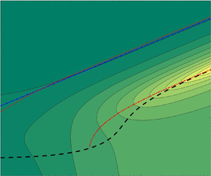
  $k_r$, for a given set of parameters. Figure 2 compares this frequency $k_r$ thus obtained with the first natural frequency computed by Floryan & Rowley (Reference Floryan and Rowley2018) from a more general theory as the mass ratio $R$ is varied. The frequency $k_{r0}$ given by (3.5) is also included, which obviously is a good approximation for large $R$, when the fluid–structure interaction becomes negligible. This agreement between $k_r$ obtained here by minimizing $|F_2|$ and that obtained numerically by Floryan & Rowley (Reference Floryan and Rowley2018) from a more general theory is a good test of the present algebraic approximation, especially considering that peak thrust forces are produced by the flexible foil at, or near, natural frequencies of the system, as shown by Floryan & Rowley (Reference Floryan and Rowley2018) and corroborated by our results in § 4 below.

Figure 2. Natural frequency  $k_r$ obtained by minimizing $|F_2|$ as a function of $R$ for $S=10$ and $a=-1$ (continuous line) compared with the first natural frequency computed by Floryan & Rowley (Reference Floryan and Rowley2018) (dashed-and-dotted line). The dashed line is $k_{r0}$ from (3.5).
Once the flexural deflection is obtained, one may compute  $C_L$ and $C_M$ using (2.24) and (2.25). These quantities are needed to obtain $C_{Li}$ and $C_{Mi}$ from (2.9) and (2.10), respectively, necessary to compute the input power coefficient,
 \begin{equation} C_P (t) = \dot{h}(t) C_{Li} (t) - 2 \dot{\alpha} (t) C_{Mi} (t), \end{equation}
which in turn is needed to obtain the propulsive efficiency. Note from (2.9) and (2.10) that this expression formally coincides with the usual one,  $C_P =-\dot {h}(t) C_{L} (t) + 2 \dot {\alpha } (t) C_{M}(t)$, for $R=0$. (Note also that here the sign of $C_M$ has been changed in relation to Alaminos-Quesada & Fernandez-Feria (Reference Alaminos-Quesada and Fernandez-Feria2020) and that, according to (2.8) and contrary to the moment, the sign of $\alpha$ is defined positive when clockwise to follow the usual convention in aerodynamics.)
Additionally, one may obtain the propulsion, or thrust, coefficient  $C_T(t)$ from the resulting deflection $d$ and the given heaving and pitching kinematics, as done above for $C_L(t)$, $C_M(t)$ and $C_F(t)$ using the quartic approximation for the deflection. In the case of a quadratic deflection like (2.7), $C_T(t)$ is given by (4.5) in Alaminos-Quesada & Fernandez-Feria (Reference Alaminos-Quesada and Fernandez-Feria2020). For the quartic deflection (2.8) the thrust coefficient is derived in a similar way, but the resulting expression becomes cumbersome. However, we have compared the time-averaged thrust values obtained with both approximations for some particular cases and found that differences are quite small, provided that the deflection $d$ is computed with the quartic approximation, as described above. For this reason, we use the expressions for $C_T$ in Alaminos-Quesada & Fernandez-Feria (Reference Alaminos-Quesada and Fernandez-Feria2020) in all the reported results.
The propulsive (Froude) efficiency is defined as
 \begin{equation} \eta = \frac{\bar{C}_T}{\bar{C}_P} , \end{equation}
where the bar denotes time-average over a period of the foil's harmonic motion,
 \begin{equation} \bar{C}_T = \frac{k}{2 {\rm \pi}} \int_t^{t+2 {\rm \pi}/k} C_T(t)\,\textrm{d}t, \end{equation}
and similarly for  $\bar {C}_P$.
The mean value of the thrust coefficient  $C_T(t)$ can be written as
 \begin{equation} \frac{\bar{C}_T}{(kh_0)^2} = t_h + t_{hp}\theta + t_p\theta^2 + \left(t_{hd} + t_{pd}\theta\right)\theta_{hd} + t_d \theta_{hd}^2, \end{equation}
with the functions  $t_h(k)$, $t_{hp}(k,a,\phi )$, $t_p(k,a)$, $t_{dh}(k,a,\psi )$, $t_{pd}(k,a,\phi ,\psi )$ and $t_d(k,a)$ given in Alaminos-Quesada & Fernandez-Feria (Reference Alaminos-Quesada and Fernandez-Feria2020), but with $p=a$ and $d_m/(1-a)^2$ substituted by $d_m$, which are reproduced in appendix B for easy reference. In this expression use has been made of the non-dimensional parameters
 \begin{equation} \theta = \frac{a_0}{k h_0} , \quad \theta_{hd} = \frac{d_m}{k h_0} , \end{equation}
where  $\theta$ is the well-known Lighthill's (Reference Lighthill1969) feathering parameter. For $\theta _{hd}=0$, we have the mean thrust coefficient $\bar {C}_T^0$ of a rigid foil with the same heaving and pitching motion (Fernandez-Feria Reference Fernandez-Feria2016, Reference Fernandez-Feria2017).
From (2.9)–(2.10) and (2.15a–c)–(2.28) substituted into (3.6), the time-averaged power coefficient can be written as
 \begin{align} \frac{\bar{C}_P}{(kh_0)^2} &= p_h + p_{hp}\theta + p_p\theta^2 + \left(p_{hd} + p_{pd}\theta\right)\theta_{hd} + R\left( p_{rhd} + p_{rpd}\theta\right)\theta_{hd}\nonumber\\ &\quad + S\left(p_{shd} + p_{spd}\theta\right)\theta_{hd}, \end{align}
where the functions  $p_h(k)$, $p_{hp}(k,a,\phi )$, $p_p(k,a)$, $p_{hd}(k,a,\psi )$, $p_{pd}(k,a,\phi ,\psi )$, $p_{rhd}(k, a,\psi )$, $p_{rpd}(k,a,\phi ,\psi )$, $p_{shd}(k,a,\psi )$ and $p_{spd}(k,a,\phi ,\psi )$ are also given in appendix B. Note that the first three terms constitute Theodorsen's power coefficient for a pitching and heaving rigid foil (Theodorsen Reference Theodorsen1935), $\bar {C}_P^0 =(k h_0)^2 [p_h(k)+ \theta \; p_{hp}(k,a,\phi ) + \theta ^2 p_p(k,a) ]$. The remaining terms are the contributions to the input power of the passive flexural deformation associated with the prescribed heaving and pitching motions (i.e. terms containing $d$ in $C_L$ and $C_M$ in the contribution of $-\dot {h} C_{L} + 2 \dot {\alpha } C_{M}$ to $C_P$), and those associated with the inertia ( $R$) and with the flexibility ( $S$) of the foil.
4. Results
4.1. Purely heaving motion with chordwise deflection
In the simplest case when no pitching motion is imposed on the foil ( $a_0=0$), the expressions (3.3)–(3.4), (3.9) and (3.11) become particularly simple. Figures 3–5 show $d_m/h_0 = k \theta _{hd}$ and $\psi$ as functions of $S$ and $k$,
$k$,  $R$ and $k$, and $a$ and $k$, respectively, for particular values of the remaining parameter in each case ( $a=-1$, $S=10$ and $R=0.01$).

Figure 3. Amplitude of the flexural component of the deflection (a) and its phase (b), both in relation to the heaving motion at the leading edge ( $a=-1$), as a function of reduced frequency $k$ and stiffness $S$ for a plate with mass ratio $R=0.01$. The dashed lines correspond to the first natural frequency of the system $k_r$ that minimizes $|F_2|$. The dotted lines in (a) are the first and second natural frequencies computed by Floryan & Rowley (Reference Floryan and Rowley2018) for this case (extracted from their figure 15).
For sufficiently large  $S$ and $k$ in figure 3, or sufficiently large $R$ and $k$ in figure 4, the amplitude of the flexural component of the deflection $d_m$ shows a marked maximum that approximately follows the first natural mode of the system, which is also plotted in these figures when obtained analytically in the present approximation by minimizing $|F_2(R,S,k,a)|$. This relation between resonance and the maximum of the flexural deflection, and then with the maximum of the thrust (see below), is in agreement with previous results of Floryan & Rowley (Reference Floryan and Rowley2018). In the present analysis, only the first natural frequency is captured since the foil's flexibility has only one degree of freedom, with a quartic deflection that approximates the shape of the first mode of an Euler–Bernoulli beam. Higher resonances are obtained by Floryan & Rowley (Reference Floryan and Rowley2018), among other authors, following the work of Wu (Reference Wu1961), where a large number of degrees of freedom are considered by expanding the deflection of the foil, and the corresponding inviscid motion around it, in a Chebyshev series with $N$ coefficients (see also Alben Reference Alben2008; Moore Reference Moore2015, Reference Moore2017; Tzezana & Breuer Reference Tzezana and Breuer2019). The present is a lowest-order model to account for the flexibility of the foil. In spite of this limitation, the great advantage of the present analysis is that an analytical solution is obtained. This situation is somewhat analogous to that considered by Moore (Reference Moore2014) for the case of a plate with infinite stiffness and finite torsional stiffness at the leading edge, where the variable is the pitching angle $a_0$ instead of the flexural deflection amplitude $d_m$, which is obtained, also analytically, in terms of the finite torsional stiffness of the leading edge instead of the finite foil's stiffness $S$ considered here. The first resonant mode of the system is, in addition, the most relevant one physically because the following modes are activated at much higher frequencies. Moreover, as shown by Alben (Reference Alben2008), the maximum possible thrust coefficient is always achieved by the flexible foil operating at or near this first resonance. Figure 3(a) also includes the natural frequency of the second mode of vibration extracted from figure 15 of Floryan & Rowley (Reference Floryan and Rowley2018) (note that their $f^*$ is the present $k/{\rm \pi}$), above which the present approximation is certainly not valid.

Figure 4. As in figure 3 but as a function of reduced frequency  $k$ and mass ratio $R$ for a plate with stiffness $S=10$. The dashed lines correspond to the first natural frequency of the system $k_r$ that minimizes $|F_2|$, while the dashed-and-dotted line is $k_{r0}$ ( $\propto R^{-1/2}$) given by (3.5), valid for for $R \gg 1$.
In figure 4, the first resonance mode for large mass ratio  $R$ is proportional to $R^{-1/2}$, in accordance with $k_{r0}$ given by (3.5) for constant $S$. Figure 5 shows that the maxima of the flexural component of the deflection amplitude for the constant values of $S$ and $R$ considered are obtained for pivots located just downstream of the mid-chord point.

Figure 5. Amplitude of the flexural component of the deflection (a) and its phase (b) as a function of reduced frequency  $k$ and the location $a$ where the heaving motion is imposed to a plate of stiffness $S=10$ and mass ratio $R=0.01$. The dashed lines correspond to the first natural frequency of the system $k_r$ that minimizes $|F_2|$.
Except for a pivot point close to the trailing edge, the local maxima in the amplitude of the flexural component of the deflection roughly correspond to local maxima in thrust and in power coefficients, since, according to (3.9)–(3.11), the thrust and power input are quadratic and linear functions, respectively, of  $d_m$. Although this is not always so because the effect of the phase, figures 6 and 7, where we plot in the stiffness–frequency plane the ratios of the time-averaged thrust and power coefficients of a flexible foil to the mean thrust and power coefficients of an otherwise identical rigid foil, respectively, clearly show that, for the selected values of $a$, the maxima in $\bar {C}_T$ and $\bar {C}_P$ approximately follow the first natural frequency, as does $d_m$. We select two different mass ratios, $R=0.01$ and $R=1$, and three different locations of the imposed heaving motion, the leading edge ( $a=-1$), the quarter-chord point ( $a=-1/2$) and the mid-chord point ( $a=0$). Though we use $h_0=0.02$ in all reported computations, except otherwise specified, the results plotted in these figures are independent of $h_0$ in the present linear theory.

Figure 6. Thrust coefficient as a function of frequency  $k$ and stiffness ratio $S$ for a heaving motion forced at different locations $a$ and with different mass ratios $R$, as labelled at the top of each panel. Lines marked with ‘0’ indicate where the flexible foil has the same thrust as the equivalent rigid foil ( $\bar {C}_T^0$). Areas with negative thrust have been whited out. The dashed lines correspond to the first natural frequency of the system $k_r$ that minimizes $|F_2|$, while the dashed-and-dotted line is $k_{r0}$ given by (3.5). The dotted line in (a) is the second natural frequency computed by Floryan & Rowley (Reference Floryan and Rowley2018) for this case (extracted from their figure 15).

Figure 7. As in figure 6 but for  $\bar {C}_P$. Areas with negative input power have been whited out.
In all cases plotted in figure 6, or in figure 7, there exists a region in the stiffness–frequency plane where the thrust, or the input power, of the flexible foil is substantially larger than that of the rigid foil counterpart. As aforementioned, these regions are always centred around the first resonance mode of the system (plotted in figures 6 and 7 with dashed lines), with the maxima in the thrust enhancement practically coinciding with this first natural frequency, like the maxima in the amplitude of the flexural component of the deflection. On the other hand, in most of the cases considered there exists a region with net drag in the low-frequency and low-stiffness range.
The regions of significant thrust enhancement by flexibility in figure 6 always lie in the large stiffness part of the plane, where the present small deflection approximation is more likely to be valid. For the case plotted in figure 6(a) ( $R=0.01$ and $a=-1$), this region practically coincides with that in figure 9(a) of Floryan & Rowley (Reference Floryan and Rowley2018) for the first resonance mode of the system (remember that their reduced frequency is our $k/{\rm \pi}$). Though Floryan & Rowley (Reference Floryan and Rowley2018) obtain results valid for higher resonance modes, the present ones are obtained analytically for given $S$,
$S$,  $R$ and the kinematics parameters. In figures 6(a) and 7(a) we also include the natural frequency of the second mode of vibration for the case $R=0.01$ with $a=-1$, extracted from figure 15 of Floryan & Rowley (Reference Floryan and Rowley2018), above which the present approximation is not valid.
For a given pivot  $x=a$, the region of thrust enhancement displaces to lower frequencies and becomes somewhat narrower as the mass ratio $R$ increases. On the other hand, as the pivot point displaces downstream along the foil for given $R$, the magnitude of the thrust enhancement by flexibility increases for the selected values of $a$ in figure 6. For $a=0$, a region of net drag is also found for frequencies higher than the first natural frequency, where the present approximation is not valid.
Similar trends are found for the power coefficient shown in figure 7, which becomes much larger than that of the rigid foil counterpart around the first resonance mode. This is also in accordance with previous results of Floryan & Rowley (Reference Floryan and Rowley2018) for  $a=-1$ and $R=0.01$ (their figure 10(a) practically coincides with figure 7(a) around the first natural mode of the system).
To see these trends more clearly for the case of  $\bar {C}_T$, figure 8 shows the maxima in the thrust enhancement, $(\bar {C}_T/\bar {C}_T^0)_{max}$, where $\bar {C}_T^0$ is the thrust of an otherwise identical rigid foil, as the pivot point location is varied for a stiffness $S=10$ and for three different mass ratios, together with the corresponding values of the frequency $k_{opt}$, which practically coincides with $k_r$. For $R$ small and unity the trends are similar, but with the maxima for each $a$ occurring at lower frequencies as $R$ increases, and with a marked peak at $a \approx 0.1$. For $R=10$ the thrust enhancement is smaller and its maximum is reached at approximately $a=0.4$, with almost no thrust enhancement for pivot point locations upstream of the mid-chord point.

Figure 8. Maxima of the thrust enhancement (a), optimal frequency (b) and thrust at the optimal frequency (c) versus the pivot point location  $a$ for three values of the mass ratio $R$, when the stiffness of the heaving foil is $S=10$.
The propulsive efficiency does not necessarily follow the same trends of  $\bar {C}_T$ and $\bar {C}_P$ because it is the ratio of two quantities with similar qualitative behaviours, with maxima at, or very close to, the first natural frequencies. In fact, it turns out that the efficiency is larger at low frequencies, almost independently of the stiffness ratio, which is also the behaviour of the rigid foil counterpart (now independently of $S$, of course). This trend of the efficiency is typical of the purely heaving motion in the linearized potential limit (e.g. Garrick's efficiency for a rigid heaving foil tends to its maximum value unity as $k \to 0$). Obviously, this is not physically valid because viscous drag is neglected in the present theory, and it is especially relevant in relation to the thrust force at low frequencies, substantially reducing the efficiency at these small frequencies, that typically becomes negative due to the viscous drag.
However, the inviscid results for the efficiency may conveniently be corrected at low frequencies by just subtracting an offset drag  $C_{D0}$ to the thrust coefficient $\bar {C}_T$ obtained with the linear potential theory (Mackowski & Williamson Reference Mackowski and Williamson2015; Fernandez-Feria Reference Fernandez-Feria2017; Floryan et al. Reference Floryan, Van Buren, Rowley and Smits2017). Offset drag $C_{D0}$ basically depends on the heaving amplitude $h_0$ and the Reynolds number, and to a lesser degree on the pivot point location, but for the small amplitudes and high Reynolds numbers for which the present theory is valid one may consider a constant value. Figure 9 shows the propulsive efficiency for a foil pivoting at the mid-chord point ( $a=0$) and two values of the mass ratio ( $R=0.01$ and $1$) when an offset drag $C_{D0}=0.05$ is used with $h_0=0.02$. It is observed that the efficiency remains positive at high frequencies, almost independently of the stiffness, a consequence of the displacement to higher frequencies of the maximum efficiency by the effect of drag. But the main effect of the offset drag on the efficiency is the appearance of a localized maximum at lower frequencies, close to the region with maximum thrust and input power around the first resonance mode of the system. The existence of these resonant peaks in efficiency as a consequence of drag is explained by Floryan & Rowley (Reference Floryan and Rowley2018), though, as for $\bar {C}_T$ and $\bar {C}_P$, we only observe here the peak associated with the first resonant mode due to the present flexural approximation. It must be noted that choosing a different value of $C_{D0}$, within its physical range around the present selected value (Floryan et al. Reference Floryan, Van Buren, Rowley and Smits2017), only modifies the efficiency at very low frequencies, leaving practically unchanged the optimal regions depicted in figure 9. If one computes the relative efficiency $\eta -\eta ^0$, where $\eta ^0$ is the efficiency of an otherwise identical rigid foil, one finds that the maxima always lie in the region of negative, or very small, efficiencies, at lower frequencies than those corresponding to the first natural mode, so that flexibility practically does not increase the propulsive efficiency in the region of large thrust enhancement. Thus, this region of thrust enhancement by flexibility near the first natural frequency for high enough stiffness almost coincides with the region of maximum efficiency, but with no relevant improvement of the efficiency in relation to a rigid foil.

Figure 9. Efficiency  $\eta$ as a function of frequency and stiffness for a heaving foil with $a=0$, $R=0.01$ (a) and $R=1$ (b), and using $h_0=0.02$ with $C_{D0}=0.05$. The dashed lines correspond to the first natural frequency of the system $k_r$ that minimizes $|F_2|$, while the dashed-and-dotted line is $k_{r0}$ given by (3.5). Areas with $\eta < -1$ have been whited out.
Based on this, in figure 10 we plot  $\eta$ at the first natural frequency $k_r$, which is a good approximation to the maximum efficiency, as a function of the pivot point location $a$ for $S=50$ and several values of the mass ratio $R$, together with the corresponding natural frequencies. Observed is an unphysical singularity at $a \approx 0.1$, also observed in figure 8 for the thrust, which is an artifact of the present linear potential model associated with a vanishing small power coefficient. Disregarding this singularity, for $R=0.01$ the model predicts a maximum efficiency in this case ( $h_0=0.02$ and $C_{D0}=0.05$) of about $0.4$ when the pivot point is close to the quarter-chord ( $a=-1/2$). As $R$ increases, the behaviour is similar, but with smaller efficiencies and a maximum attained for increasing $a$ when $a <0$. For $a \gtrsim 0.1$, the efficiency is negative or very small. In fact, the singularity roughly marks the pivot point location downstream of which the flexible heaving foil is not efficient for propulsion.

Figure 10. Efficiency at  $k=k_r$ as a function of the pivot point location (a) and the corresponding $k_r$ (b) for $S=50$ and three values of $R$, for a purely heaving motion with $h_0=0.02$ and $C_{D0}=0.05$.
This behaviour is corroborated for all values of the stiffness  $S$ in figure 11, which shows $\eta$ at $k=k_r$ in the $S$–
$S$– $a$ plane for $R=0.01$ and $R=1$, together with the corresponding values of $k_r$. For $-1 < a \lesssim 0$, the maximum efficiency for constant $R$ is attained at values of the stiffness $S$ that decrease almost linearly with $a$. Curiously, this linear band of maximum efficiency in the $S$–
$S$– $a$ plane practically corresponds to a constant value of $k_r$. For $R=0.01$, the maximum of $\eta$ within this band is reached for a pivot point close to the the mid-chord with $S \approx 10$ (disregarding the singularity at $a \approx 0.1$ mentioned above, which has been whited out in figure 11, together with negative values of the efficiency), while for $R=1$ the maximum is attained for a pivot point approaching the leading edge for a value of $S$ larger than $100$. In fact, a local maximum of $\eta$ exists at $a=-1$ for both values of $R$ at sufficiently high values of $S$ (larger than $100$). Given its physical relevance within the present approach, valid for large $S$, this local maximum is characterized in figure 12. This figure shows that the maximum efficiency for a foil pivoting at the leading edge in the present case is approximately $0.44$, attained for $R \simeq 10$ and $S \approx 430$ with an operating frequency $k \simeq 3.13$. Figure 11 also shows that for $a \gtrsim 0.1$ the efficiency is negative or very low, as already discussed in relation to figure 10 for $S=10$, except for small $S$ for which the present theory is not valid.

Figure 11. Efficiency at  $k=k_r$ (a,c) and the corresponding $k_r$ (b,d) in the stiffness–pivot point location plane for a purely heaving motion with $h_0=0.02$ and $C_{D0}=0.05$, for $R=0.01$ (a,b) and $R=1$ (c,d). Areas with negative efficiency have been whited out.

Figure 12. Maxima in the efficiency versus the mass ratio for a heaving motion pivoting at the leading edge (a) and the corresponding values of the stiffness and frequency (b). Here  $h_0=0.02$ and $C_{D0} =0.05$.
4.2. Purely pitching motion with chordwise deflection
For a foil with mass ratio  $R$ undergoing a purely pitching motion of small amplitude $a_0$ about a pivot point location $a$, the effect of flexibility on the propulsive performance is qualitatively similar in the stiffness–frequency plane to that described above for a heaving motion with the same $a$ and $R$. The pitching motion just generates smaller maxima of the flexural deflection amplitude than that from the equivalent heaving motion, in relation to their rigid foil counterparts, and consequently less thrust enhancement by flexibility.
As an example, figure 13(a) shows, in the stiffness–frequency plane, the ratio of the time-averaged thrust of a flexible foil to the mean thrust coefficient of an otherwise identical rigid foil for  $R=0.01$, $a=-1$ and $a_0=2^{\circ }$, though the plotted results are independent of the pitching amplitude $a_0$. The region of substantial thrust enhancement by flexibility is similar to that in figure 9(b) of Floryan & Rowley (Reference Floryan and Rowley2018) around the first resonance mode of the system (which is also plotted as a dotted line). Figure 13(b) shows the propulsive efficiency for the same case, but now using an offset drag $C_{D0}=0.05$. As in the case of purely heaving motion, there is a region of maximum efficiency close to the thrust enhancement region around the first natural mode.

Figure 13. Thrust coefficient (a) and efficiency (b) as a function of frequency  $k$ and stiffness ratio $S$ for a pitching motion about the leading edge ( $a=-1$) with $R=0.01$ ( $a_0=2^{\circ }$ and $C_{D0}=0.05$). The lines marked with ‘0’ in (a) indicate where the flexible foil has the same thrust as the equivalent rigid foil ( $\bar {C}_T^0$). Areas with negative thrust have been whited out in (a), while values less than $-2$ are whited out in (b). The dashed lines correspond to the first natural frequency of the system $k_r$ that minimizes $|F_2|$, while the dashed-and-dotted line in (a) is $k_{r0}$ given by (3.5). The dotted lines are the second natural frequency computed by Floryan & Rowley (Reference Floryan and Rowley2018) for this case (extracted from their figure 15).
Figure 14 shows the propulsive efficiency at  $k=k_r$ as $a$ is varied for $S=10$ and several values of $R$, together with the corresponding values of $k_r$. It is observed that the efficiency predicted by the model becomes singular in certain narrow intervals of $a$ containing $a=0$ that depends on $R$ and $S$; within these ranges of $a$ the present approximation with a small quartic deflection is not valid. For pivot locations upstream of these singular intervals, the efficiency reaches a maximum that decreases with increasing $R$ at practically the same value of $a$ (
$a$ ( $\simeq 0.17$ in the plotted cases). For pivot locations downstream of the singular narrow region, the efficiency is negative or very low. Therefore, the singularity marks again the pivot point locations downstream of which the propulsive efficiency of the flexible (now pitching) foil becomes poor. The difference from the heaving foil case discussed above is that now there exists a narrow region of pivot point locations that depends on $S$ and $R$, instead of being an almost constant pivot point location ( $a \approx 0.1$) as $S$ and $R$ are varied.

Figure 14. Efficiency at  $k=k_r$ (a) and the corresponding $k_r$ (b) versus $a$ for a pitching motion with $a_0=2^{\circ }$ and $C_{D0}=0.05$, for $S=10$ and three values of $R$.
$R$.
Indeed, this is observed in figure 15, which shows the effect of the stiffness  $S$ on the efficiency at $k=k_r$ for the case with $R=0.01$ in figure 14. The singular regions and those with negative efficiency have been whited out in the $a$–
$a$– $S$ plane. As the pivot location moves from the leading edge to the singularity close to the mid-chord point, the maxima in the efficiency are attained at decreasing values of $S$, starting close to $100$ for $a=-1$. For pivot point locations downstream of the singular region, the efficiency is negative or very low for all the range of values of $S$ considered. Figure 16 shows the evolution with the mass ratio $R$ of the maximum in the efficiency when the pivot point is at the leading edge ( $a=-1$), together with the corresponding values of $S$ and $k_r$.

Figure 15. Efficiency at  $k=k_r$ (a) and and the corresponding frequencies (b) in the stiffness–pivot point location plane for a purely pitching motion with $a_0=2^{\circ }$ and $C_{D0}=0.05$ for $R=0.01$. Areas with negative or singular efficiency have been whited out.

Figure 16. Maxima in the efficiency versus the mass ratio (a) and the corresponding values of the stiffness and frequency (b) for a pitching motion about the leading edge with  $a_0=2^{\circ }$ and $C_{D0} =0.05$.
4.3. Pitching and heaving motion about the leading edge
Finally, as an example of combined pitching and heaving motions we only present results for the case in which they are forced at the leading edge ( $a=-1$), and just to see how an appropriate addition of pitching to a heaving motion may significantly increase both the thrust and the propulsive efficiency of the foil, additionally to that caused by flexibility discussed above, as is well known for rigid flapping foils (Anderson et al. Reference Anderson, Streitlien, Barret and Triantafyllou1998).
To that end we select the case with the highest propulsive efficiency for a heaving foil with  $R=0.01$ when $h_0=0.02$, $C_{D0}=0.05$ and $a=-1$, which according to figure 12 is approximately $40\,\%$ when $k \simeq 6.9$ and $S$ about $130$. Figure 17 shows the thrust and efficiency enhancement in relation to the corresponding heaving-only foil, $\bar {C}_{T}/\bar {C}_{Th}$ and $\eta -\eta _{h}$, respectively, when pitching motions of increasing amplitude $a_0$ and phase shift $\phi$ are added.

Figure 17. Thrust (a) and efficiency (b) enhancement by adding a pitching motion about the leading edge ( $a=-1$) of amplitude $a_0$ and phase shift $\phi$, in relation to the thrust and efficiency of the heaving-only motion, $\bar {C}_{Th} \simeq 0.378$ and $\eta _{h} \simeq 0.4$, respectively, with $h_0=0.02$ and $C_{D0}=0.05$, for a foil with $R=0.01$ and $S=130$, and a reduced frequency $k=6.9$. The contour values in (b) are for $(\eta - \eta _h) \times 100$.
Any amount of pitching, even of infinitesimal amplitude, increases the thrust generated by the foil provided that its phase shift  $\phi$ in relation to the heaving motion is appropriate. For small $a_0$, this happens in this case when $90^{\circ } \lesssim \phi \lesssim 270^{\circ }$, with the thrust enhancement maximized at $\phi \approx 180^{\circ }$. In relation to the efficiency, figure 17(b) shows that there exists a threshold in the pitch amplitude above which the efficiency improves in relation to the heaving-only motion. For the present case with very small $h_0$, this minimum amplitude is also very small, about $0.2^{\circ }$, generating thrust enhancement for a phase shift $\phi$ of about $204^{\circ }$. As the amplitude $a_0$ increases, the optimal phase shift for efficiency enhancement increases, approaching $360^{\circ }$ (i.e. $0^{\circ }$) for sufficiently high amplitude.
5. Concluding remarks
We derive analytical expressions for the propulsive performance of a two-dimensional foil with prescribed pitching and heaving motions about arbitrary pivot points when a quartic chordwise deflection is allowed to accommodate passively to the fluid–structure interactions. The formulation is limited to high Reynolds numbers (inviscid flow), small amplitudes of the foil motion (no flow separation) and large stiffness combined with low-to-moderate reduced frequencies and mass ratios, so that only the first resonant mode of the system is activated. The formulation incorporates the effect of the inertia of the solid foil on both the thrust and input power, and therefore on the propulsive efficiency, directly from the Euler–Bernoulli beam equation, an effect that becomes relevant when the mass ratio is not small. Thus, the results are valid for modelling both swimming and flying applications of flapping foils.
The present formulation uses a slightly modified form of the purely kinematic results in Alaminos-Quesada & Fernandez-Feria (Reference Alaminos-Quesada and Fernandez-Feria2020) for a quadratic deflection to compute the flexural deflection amplitude and its phase in terms of the solid foil properties, namely its dimensionless stiffness and mass ratio, in addition to all the kinematic parameters associated with the forced heaving and pitching motion applied at an arbitrary pivot point. The maximum flexural deflection amplitude is found to be attained at, or near, the first natural frequency of the system, which is also obtained here algebraically, being the only natural frequency recovered in the present approximation. At this frequency, which depends on the stiffness, mass ratio and the location of the pivot point, the thrust and power input also reach their respective maximum values, approximately, though not necessarily the propulsive efficiency. These results are in agreement with previous numerical results for purely heaving and pitching motions about the leading edge ( $a=-1$) for low mass ratios ( $R=0.01$) reported by Floryan & Rowley (Reference Floryan and Rowley2018), though the formulation by those authors accounts for the whole series of natural frequencies of the system, depending on the number of terms retained in the Chebyshev expansion. In this sense, the present approach is equivalent to the lowest order of this expansion formulated through the first three moments of the Euler–Bernoulli beam equation, thus constituting a minimal model of the flexible foil. Though the limitation to (small-amplitude) quartic deformations restricts the theory to include only the first resonant frequency of the system, as shown by Alben (Reference Alben2008) from a similar linear potential flow theory, the maximum possible thrust coefficient is always achieved by the flexible foil operating at or near this first resonance. The cases of purely heaving and purely pitching motions are analysed with detail in the present work, characterizing the parametric ranges generating maximum thrust and maximum propulsive efficiency enhancement as the stiffness of the foil is varied, including the effect of the pivot point location for a wide range of mass ratios.
Though results are presented for a foil with uniform thickness, chordwise rigidity and density, the analytical results are easily generalized to account for any chordwise distribution of the non-dimensional stiffness  $S(x)$ and the mass ratio $R(x)$ using (2.4)–(2.6). More complicated motions of the foil, with additional kinematic parameters, could also be considered within the present approach by including additional moments of the Euler–Bernoulli equation, though then the resulting analytical expressions, if attainable, would become much more involved and probably would not have any advantage over the method based on Chebyshev expansions.
Acknowledgements
The authors are grateful for the useful comments of an anonymous reviewer that have greatly improved the paper.
Funding
This research has been supported by grants from the Ministerio de Ciencia e Innovación of Spain (DPI2016-76151-C2-1-R and PID2019-104938RB-I00) and from the Junta de Andalucía, Spain (UMA18-FEDER-JA-047 and P18-FR-1532).
Declaration of interests
The authors report no conflict of interest.
Appendix A. Equation (2.1)
As commented on just below the Euler–Bernoulli beam equation (2.1), in addition to the usual continuous pressure distribution considered in the references given above it, we have included terms modelling localized force and torque at the pivot point  $x=a$ through Dirac's delta function and its derivative. Though we have not seen this equation written down in that way previously, modelling a punctual force through Dirac's delta function $\delta$ is a normal practice in dynamics. Likewise, a punctual (clockwise) torque can be modelled by its derivative $\delta '$. Since these functions satisfy the properties (the second one just by integrating by parts, see e.g. Lighthill (Reference Lighthill1958))
 \begin{equation} \int_{-\infty}^{\infty} \delta(x-a) F(x)\,{\textrm{d}x} = F(a), \quad \int_{-\infty}^{\infty} \delta'(x-a) F(x)\,{\textrm{d}x} = - F'(a), \end{equation}
one readily recovers the right-hand sides of (2.4) and (2.5).
Appendix B. Functions for the time-averaged coefficients
B.1. Thrust coefficient
The functions  $t_h(k)$, $t_{hp}(k,a,\phi )$, $t_p(k,a)$, $t_{hd}(k,p,\psi )$, $t_{pd}(k,a,p,\phi ,\psi )$ and $t_d(k,p)$ appearing in the time-averaged thrust coefficient (3.9) are the following:
 \begin{gather} t_h(k) =-2\mathcal{G}_1(k), \end{gather}
 \begin{gather} t_{hp}(k,a,\phi) = \left[(3-4 a)\mathcal{G}_1 k - 2 \mathcal{F}_1\right]\cos (\phi )+ (2 \mathcal{G}_1-\mathcal{F}_1 k)\sin (\phi ), \end{gather}
 \begin{gather} t_{p}(k,a) = 2 (1-a) k \left[\mathcal{F}_1-\left(\frac{1}{2}-a\right) \mathcal{G}_1 k\right], \end{gather}
 \begin{gather} t_{d}(k,a) = k (1-a)^2 \left\{4 \mathcal{F}_1 \left(\frac{1}{2}-a\right)- \mathcal{G}_1 k [1+2 (a-1) a]\right\}, \end{gather}
 \begin{gather} t_{hd}(k,a,\psi) = 4 \left\{ \left(a-\frac{1}{2}\right)\left(\mathcal{G}_1-\frac{\mathcal{F}_1 k}{2}\right)\sin (\psi ) \right.\nonumber\\ \quad + \left. \left[ \mathcal{F}_1 \left(\frac{1}{2}-a\right)-\mathcal{G}_1 k \left(a^2-\frac{3}{2}a+\frac{3}{4}\right) \right] \cos (\psi ) \right\}, \end{gather}
 \begin{gather} t_{pd}(k,a,\phi,\psi) = k \left\{ \left[ 4 \left( - \frac{3}{2} a^2 + \frac{5}{2} a -1 \right) \mathcal{F}_1 \right. \right.\nonumber\\ \quad + \left. \left. 4 k \left( -a^3+\frac{9}{4} a^2 - \frac{7}{4} a +\frac{1}{2}\right)\mathcal{G}_1 \right]\cos (\phi -\psi )\right.\notag\\ \quad + \left. a (1-a) (2 \mathcal{G}_1-\mathcal{F}_1 k) \sin (\phi -\psi ) \right\}. \end{gather}
Here  $\mathcal {F}(k)$ and $\mathcal {G}(k)$ are the real and imaginary parts of Theodorsen's function (2.28) and
 \begin{equation} \mathcal{C}_1(k) = \frac{\dfrac{1}{k}\textrm{e}^{-\textrm{i}k}}{\textrm{i}H_0^{(2)}(k) + H_{1}^{(2)}(k)} := \mathcal{F}_1(k)+\textrm{i}\mathcal{G}_1(k) . \end{equation}
B.2. Power coefficient
The the functions  $p_h(k)$, $p_{hp}(k,a,\phi )$, $p_p(k,a)$, $p_{hd}(k,a,\psi )$, $p_{pd}(k,a,\phi ,\psi )$, $p_{rhd}(k,a,\psi )$, $p_{rpd}(k,a,\phi ,\psi )$, $p_{shd}(k,a,\psi )$ and $p_{spd}(k,a,\phi ,\psi )$ appearing in the power coefficient (3.11) are the following:
 \begin{gather} p_h = {\rm \pi}\mathcal{F}, \end{gather}
 \begin{gather} p_{hp} = {\rm \pi}\left[\left(2 a \mathcal{F} k-\mathcal{G}-\frac{k}{2}\right)\cos (\phi )+(\mathcal{G} k-\mathcal{F})\sin (\phi ) \right], \end{gather}
 \begin{gather} p_{p} = {\rm \pi}k \left[\left(a^2-\frac{1}{4}\right) \mathcal{F} k-\left(a+\frac{1}{2}\right) \mathcal{G}+\frac{1}{2} \left(\frac{1}{2}-a\right) k\right], \end{gather}
 \begin{align} p_{hd} &= {\rm \pi}\left[\mathcal{F} k \left(A-\frac{B}{2}+\frac{D}{2}-\frac{3 (E-J)}{8}\right)-\mathcal{G} \left(B-D+\frac{3 (E-J)}{2}\right)\right.\nonumber\\ &\quad - \left.\frac{k}{2} \left(B+\frac{3 E}{4}\right)\right]\cos (\psi ) + {\rm \pi}\left[\mathcal{G} k \left(\frac{B}{2}-\frac{D}{2}+\frac{3 (E-J)}{8}-A\right)\right.\nonumber\\ &\quad - \left. \frac{k^2}{2} \left(A+\frac{D}{4}+\frac{J}{8}\right)-\mathcal{F} \left(B-D+\frac{3 (E-J)}{2}\right)\right]\sin (\psi ), \end{align}
 \begin{align} p_{pd} &= {\rm \pi}\left\{\left(a+\frac{1}{2}\right) \mathcal{F} k \left(A-\frac{B}{2}+\frac{D}{2}-\frac{3 (E-J)}{8}\right)\right.\nonumber\\&\quad + \left(a+\frac{1}{2}\right) \mathcal{G} \left(-B+D-\frac{3 (E-J)}{2}\right) \nonumber\\&\quad + \left. \frac{k}{2}\left[\left(\frac{1}{2}-a\right) \left(B+\frac{3 E}{4}\right)-\frac{D}{2}-\frac{J}{2}\right]\right\}\cos (\phi -\psi )\nonumber\\&\quad + \ {\rm \pi}\left\{\left(a+\frac{1}{2}\right) \mathcal{G} k \left(A\!-\!\frac{B}{2}+\frac{D}{2}\!-\!\frac{3 (E-J)}{8}\right) + \left(a\!+\!\frac{1}{2}\right) \mathcal{F} \left(B\!-\!D+\frac{3 (E\!-\!J)}{2}\right) \right.\nonumber\\&\quad + \left. \frac{D}{2}-\frac{3 E}{8}+\frac{3 J}{4}+\frac{k^2}{2} \left[a \left(A+\frac{D}{4}+\frac{J}{8}\right)+\frac{B}{8}+\frac{E}{16}\right]\right\}\sin(\phi -\psi ), \end{align}
 \begin{gather} p_{rhd} = -2k^2 s_{l}(a) \sin (\psi ), \end{gather}
 \begin{gather} p_{rpd} = 2k^3 s_{m}(a) \sin (\phi -\psi ), \end{gather}
 \begin{gather} p_{shd} = -\frac{8\sin (\psi )}{3 (1-a)^2}, \end{gather}
 \begin{gather} p_{spd} = \frac{8 a k \sin (\phi -\psi )}{3 (1-a)^2}, \end{gather}
where  $s_l$, $s_m$, $A$,
$A$,  $B$,
$B$,  $D$,
$D$,  $E$ and $J$ are the functions of $a$ defined in (2.12)–(2.13) and (2.21a,b)–(2.22a–c).


 Open access