


1. Introduction
1.1. Context
IFRS 17 Insurance Contracts is a new accounting standard that entities are expected to apply for reporting periods beginning on or after 1 January 2023 (though earlier application is permitted). It supersedes IFRS 4 Insurance Contracts.
IFRS 17 establishes key principles that entities must apply in all aspects of the accounting of insurance contracts (e.g. recognition, measurement, presentation and disclosure). In doing so, the Standard aims to increase the usefulness, comparability, transparency and quality of insurers’ financial statements.
A fundamental concept introduced by IFRS 17 is the contractual service margin (CSM). The CSM, in most instances, represents the unearned profit that an entity expects to earn as it provides services.Footnote 1 However, as a principles-based standard, IFRS 17 results in entities having to apply significant judgement when determining the inputs, assumptions and techniques it uses to determine the CSM at each reporting period. Indeed, several aspects of the Standard have been left open for the entities to determine what approach they consider to best reflect the effect of insurance contracts on their financial position and performance. Important examples of areas where such judgement is required include the level of aggregation; the identification of contract boundaries; the determination of coverage units; the treatment of loss components (LC) and the treatment of with-profits (WP) funds. In addition to issues pertaining to judgement, there are requirements of the Standard that may create economic or accounting mismatches.
The IFRS 17 CSM Working Party was one of the three working parties established by the Life BoardFootnote 2 of the IFoA in the summer of 2018 in anticipation of the diversity of interpretation and application of the Standard. There is also a fourth working party that looks at IFRS 17 issues in the non-life space.Footnote 3 Each working party focuses on different aspects and challenges of IFRS 17 and consequently, there are few areas of overlap; our group’s objective is to analyse the technical, operational and commercial impacts of different approaches to calculating the CSM at initial recognition and subsequent measurement from a life insurance perspective.
As a standard that is still very much in its infancy, and for which wider consensus on topics is yet to be achieved, this paper aims to provide readers with a deeper understanding of the issues pertaining to the CSM and the opportunities that accompany it.
1.2. Intended Audience
The working party expects this paper to sit most comfortably in the hands (or on the screens) of readers who have prior knowledge of IFRS 17 and are broadly familiar with its various concepts and themes. However, readers with less familiarity than this need not be repelled; the paper attempts to provide sufficient exposition of the requirements (with examples where possible) to help facilitate engagement with the material presented. Experienced IFRS 17 practitioners, who already have an intimate awareness of issues, may find this paper useful to validate their own conclusions or pick up on new points of detail.
1.3. Scope
This paper aims to focus solely on issues pertaining to the CSM. As such, it is neither intended, nor should be read as, an exhaustive IFRS 17 manual. As the first truly international accounting standard for insurance contracts, IFRS 17 embeds within it an enormous amount of complexity and touches on substantial topics for which entire papers could be dedicated in their own right (e.g. discount rates or the risk adjustment (RA)). For this reason, the paper has had to be necessarily restricted to the CSM in its scope. As examples, the paper does not touch on any of the following issues in detail except to the extent that there are some points of tangential relevance to the CSM (if at all):
-
Possible approaches to determining the RA.
-
Considerations relating to the premium allocation approach (PAA).
-
Identification of non-distinct investment components (NDIC).
-
Treatment of acquisition costs.
-
Disclosures and presentation requirements.
-
Accounting policy choices available under IFRS 17 (e.g. OCI disaggregation; presentation of the RA in the P&L; treatment of accounting estimates made in previous reporting periods, etc.).
-
IFRS 9 requirements.
-
Designing systems and processes to comply with the Standard.
In some instances, there will be topics that our sister working parties are dedicated to examining in much more detail than considered in this paper. Here, as above, the approach taken is to only cover angles relevant to the CSM and not to cover the topic more widely. For example:
-
“How should discount rates be set based on a top-down or bottom-up approach?” is a broader question being addressed in detail by the Discount Rates working party, but “what impact does using different weighted average yield curves have on the CSM?” is a specific question that is considered in this paper
-
“What impact does IFRS 17 have on KPIs?” is a question relevant for the Transversal working party, but “what impact does the CSM have on return-on-equity?” is a specific question that is considered in this paper
1.4. Structure of the Paper
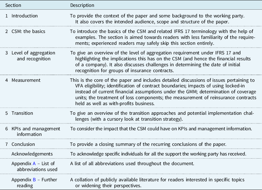
The paper consists of seven main sections followed by acknowledgements and two appendices as shown in Table 1.
Table 1. Structure of the Paper
1.5. IFRS 17 References in the Paper
The paper references IFRS 17 paragraphs from the following sources:
-
“IFRS 17 Insurance Contracts” – incorporating all amendments as issued in June 2020Footnote 4 .
-
“Basis for Conclusions on IFRS 17” as issued in May 2017.
-
“Basis for Conclusions on Exposure Draft Amendments to IFRS 17” as issued in June 2019.
-
“Illustrative examples on IFRS 17” as issued in May 2017.
The paper’s approach of referring to IFRS 17 paragraphs will differ depending on the issue being covered. In many instances, it was considered sufficient to merely refer to the paragraph numbers (most of which can be found in the link in the footnote); in some instances, it was deemed more helpful to provide extracts of the paragraphs themselves; elsewhere it was judged to be appropriate to summarise the paragraphs.
2. CSM: The Basics
Section 2 covers the basics of the CSM. The section is aimed towards less familiar readers; experienced audiences may safely skip this section entirely.
2.1. Introducing the Logic of the CSMFootnote 5
The discussion starts with an introduction to the logic of the CSM. It proceeds in four parts:
-
CSM at initial recognition.
-
CSM at subsequent measurement.
-
CSM for reinsurance contracts held.
-
Recognition of the CSM in profit or loss.
By the end of section 2, less familiar readers will become acquainted with the fundamental ideas underpinning the CSM.
2.1.1. CSM at initial recognition
Consider what happens under an economic balance sheet (e.g. SII for the most part) when an insurer writes a new contract – if the contract is profitable, the insurer recognises a negative liability (effectively an asset) but if the contract is loss-making, the insurer recognises a positive liability. In either case, an economic view results in insurers capitalising, at the point of sale, the total profits or losses expected to be made under those contracts over their lifetimes.
The recognition of profits or losses under IFRS 17 begins with two deliberate, asymmetric principles that are intended to depart from this economic view.
Principle 1: When an insurer writes profitable business, it must not be allowed to recognise the expected profits for that business immediately and instead must spread those profits over time (based on paragraph 38).
Principle 2: When an insurer writes loss-making business, it must not be allowed to spread the expected losses for that business over time and instead must recognise those losses immediately (based on paragraph 47).
The CSM is a fundamental concept introduced by IFRS 17 that embodies these principles at its core.
Under Principle 1, when an insurer writes profitable business, it is forced to avoid the day 1 recognition of profits through the establishment of a CSM. The CSM, in turn, can only be recognised in the profit or loss statement on a gradual and systematic basis over time, as and when insurance services are provided. At any given reporting period, the CSM consequently represents the expected amount of profits that have not yet been earned under the group of contracts in question.
Under Principle 2, when an insurer writes loss-making business, it cannot establish a “negative CSM” and defer loss recognition into the future. This is because the CSM is floored to zero in such circumstances.
These principles can be illustrated using simplified examples as shown in Tables 2 and 3.
Table 2. Example of CSM Calculation at Initial Recognition for Profitable Contracts
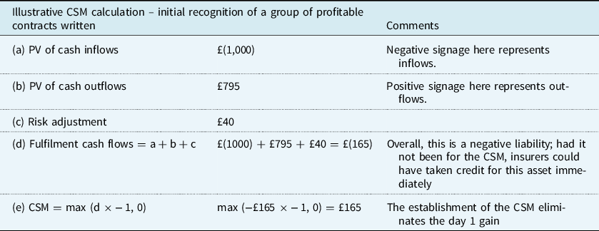
Table 3. Example of CSM Calculation at Initial Recognition for Loss-Making Contracts

At initial recognition, before any cash flows are exchanged, the two principles above would stack up as shown in Figure 1.

Figure 1. Illustration of the contractual service margin at initial recognition.
2.1.2. CSM at subsequent measurement
Insurance business is almost invariably exposed both to the impacts of emerging experience being different to that expected and to the impacts of assumptions relating to future experience being different to that previously assumed. It stands to reason that the CSM – i.e. the balance that represents unearned profits – ought to be updated to reflect these latest facts and circumstances. IFRS 17 acknowledges both these classes of items by referring to them as “changes that relate to future service”.
Principle 3: With some exceptions (which need not be addressed in this introduction), the CSM must be adjusted for all changes that relate to future service – e.g. favourable mortality updates must increase the CSM; unfavourable lapse experience must decrease the CSM (based on paragraphs 44(c) and 45(c)).
An example is shown in Table 4.
Table 4. Example of CSM Adjustment for Changes Relating to Future Service

Occasionally, there may be unfavourable changes relating to future service that happen to be larger than the CSM even after accreting for interest. How should these be accounted for? The logic of IFRS 17 continues.
Principle 4: When an insurer recognises that written business, that was previously expected to be profitable, is now expected to be loss-making, e.g. because of changes relating to future service, it must not be allowed to spread the expected losses for that business over time and instead must recognise those losses immediately. It will do so by first extinguishing the CSM and then establishing a LC in respect of the remaining excess (based on paragraphs 44(c) and 45(c)).
Principle 4 consequently extends the scope of Principle 2 so that it can apply to the measurement of the CSM subsequent reporting periods. Even at subsequent measurement, the insurer is not allowed to establish a negative CSM and defer loss recognition, instead, it must recognise such excess losses immediately.
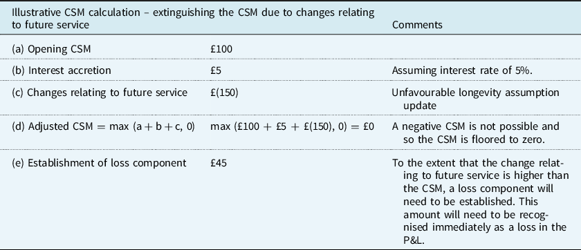
An example is shown in Table 5.
Table 5. Example of CSM Extinguished due to Changes Relating to Future Service
2.1.3. CSM for reinsurance contracts held
The principles discussed so far apply equally to insurance contracts written by insurers as well as reinsurance contracts written by reinsurers. However, in recognition of the fact that concepts such as unearned profit or onerousness cannot apply to reinsurance contracts held, IFRS 17 modifies some of these principles in important ways to better accommodate such contracts.
Principle 5: With some exceptions (only one of which is deemed important to this introduction – see below), when an insurer (or reinsurer) purchases reinsurance, it must not be allowed to recognise the expected net cost or net gain for that contract immediately, instead, it must spread that net cost or net gain over time (based on paragraph 65).
Principle 5 consequently modifies the logic of Principle 1 to make it appropriate for reinsurance held: when an insurer (or reinsurer) purchases reinsurance, it is forced to avoid the immediate recognition of not only the expected cost of that reinsurance, but also any expected gains. In other words, reinsurance CSM, unlike the gross underlying CSM, has no floor and can have either positive or negative signage. An example of this calculation is shown in Table 6.
Table 6. Example of Reinsurance CSM Calculation at Initial Recognition for Reinsurance Contracts held

The reinsurance CSM can only be recognised in the profit or loss statement on a gradual and systematic basis over time, as and when reinsurance services are received. At any given reporting period, the reinsurance CSM consequently represents the expected amount of costs or gains that have not yet been recognised for the group of reinsurance contracts in question. Just like the gross underlying CSM, the reinsurance CSM also needs to be adjusted for all changes relating to future service (with some exceptions).
One important exception relating to Principle 5 concerns an issue relating to the interaction between gross underlying business and corresponding reinsurance held. Consider an insurer that has just written a loss-making contract and, as per Principle 2, recognises an immediate P&L hit of £35 (say). However, the insurer already holds an external reinsurance contract under which this contract is 100% reinsured on an original terms quota share basis. Principle 5 on its own would imply that a (net gain) reinsurance CSM of £35 would be established and spread over time. However, this results in a timing mismatch: even though gross underlying claims are effectively capitalised and recognised on day 1 in recognising the upfront loss, the corresponding reinsurance recoveries cannot be taken credit for immediately. The exception to Principle 5 is designed to avoid this mismatch from arising.
Exception to Principle 5: If an insurer (or reinsurer) has purchased a reinsurance contract either before, or at the same time as, it recognises a loss for a loss-making underlying contract, the insurer must recognise reinsurance income to offset (in full or in part) the underlying loss recognised. The insurer shall adjust the reinsurance CSM to reflect that credit for future claim recoveries has already been taken by recognising income (based on paragraphs 65 and 66A).
2.1.4. Recognition of the CSM in profit or loss
One final point of detail remains to be covered. Earlier, it was noted that the CSM can only be recognised in the profit or loss statement on a gradual and systematic basis over time, as and when insurance services are provided. Why is this required and what does it mean in practice?
Why is this required?
IFRS 17 Effects Analysis answers this question best:
“Currently, insurers recognise profits inconsistently over time. The timing of recognition of profit for insurance services can vary significantly by jurisdiction and by product. Some insurers recognise profit immediately when an insurance contract is written. Other insurers recognise profit only when the contract terminates. Other insurers recognise profit over the duration of the insurance contract on the basis of the passage of time.” (IFRS 17 Effects Analysis, page 33)
Consider an immediate annuity contract with a single premium paid by the policyholder at the outset of the contract in return for fixed regular annuity payments for the remainder of the policyholder’s life. The insurer that writes this contract expects to make a profit:
-
Recognising all this expected profit upfront creates a large disconnect with the fact that insurance service is likely to be provided over several years to come.
-
Waiting for all this profit to be recognised only when the policyholder dies is problematic because companies would have to wait for several decades before being able to recognise a return on their investments.
-
Recognising this profit systematically over time avoids both extremes and enables the possibility for a reasonable link to be secured between the rate at which profit is recognised and the amount of insurance service provided over time.
What does this mean in practice?
To determine how much profit should be recognised in each period, the entity is required to identify the number of “coverage units”. In effect, coverage units are an attempt to quantify the amount of insurance services provided to groups of contracts. They are determined by considering the “quantity of benefits” provided under contracts and how long on average the contracts are expected to last.
Take a simplified example of a 5-year term assurance contract with a sum assured of £100. The calculations for this example are shown in Table 7.
Table 7. Example of CSM Amortisation Calculations

After allowing for the expected lapse and mortality decrements, the insurer arrives at a view of sum assured that is expected to remain in force for each projection year (see column A). The insurer takes the view that the sum assured in force is an appropriate measure for the quantity of benefits and consequently uses this for its coverage units (see column B). It aggregates total coverage units expected to be provided in all years (see column C). It calculates an “amortisation ratio” by expressing coverage units in the current year as a percentage of total coverage units remaining to be provided (see column D).
Once the amortisation ratio is determined, it is applied to the CSM: the amount by which the CSM is reduced through this amortisation is recognised as profit in the P&L.
An example of the CSM release in profit or loss calculation is shown in Table 8.
Table 8. Example of CSM Recognition Calculation

Coverage units, just like the CSM, need to be reassessed at subsequent periods because of changes relating to future service.
In the fifth and final year of the simplified term assurance contract above, the amortisation rate is 100%. Applying this to the CSM results in a closing CSM of zero indicating that no further service remains to be provided and consequently no unearned profits left to recognise.
This concludes the introduction to the logic of the CSM.
2.2. How is the CSM Calculated?
This paper has briefly touched on how the CSM is calculated in section 2.1 but will now consider this question in this section in more detail.
CSM at initial recognition
For all types of insurance products, the CSM at initial recognition for a group of written contracts is calculated as shown in Table 9.
Table 9. Steps for Calculating the CSM at Initial Recognition

Note in this calculation:
-
The present value computation is based on the appropriate IFRS 17 discount rate. Unlike SII, IFRS 17 does not prescribe discount rates and companies are responsible for determining their own discount rates that, amongst other things, “reflect…the characteristics of the cash flows and the liquidity characteristics of the insurance contracts” (paragraph 36). The setting of discount rates is a substantial topic in its own right, and, apart from some issues immediately relevant to the CSM, is not addressed in much detail in this paper.
-
Cash flows expected in the future should only take account of cash flows that fall within the IFRS 17 contract boundary (paragraph 33). The determination of contract boundaries under IFRS 17 is not always straightforward and cannot be assumed to follow SII contract boundaries – this is explored further in section 4.3.
-
Cash flows at the date of initial recognition include initial premiums as well as directly attributable acquisition cash flows. The date of initial recognition has a specific sense under IFRS 17 (paragraph 25) and there are challenges around determining it – these are addressed in section 3.3.
-
The RA for non-financial risk reflects “uncertainty about the amount and timing of the cash flows that arises from non-financial risk” (paragraph 37). The RA under IFRS 17 has overlapping features with the risk margin under SII however there are important differences. Most notably, unlike SII, the calculation of the RA is not prescribed under IFRS 17 and consequently, it is up to companies to determine for themselves the techniques they will use to calculate the RA. The RA is a substantial topic in its own right, and, with some exceptions, is not addressed in any detail in this paper.
-
The “asset for insurance acquisition cash flows” is a newly introduced concept under IFRS 17. It is important to note this asset is not the same as the DAC (deferred acquisition cost) asset that readers may already be familiar with (e.g. from IFRS 4). The purpose of this new asset is to enable an allocation of incurred acquisition costs to future new business. For many life companies, this new asset will not need to be established (the situation differs for non-life companies) however it is sufficient to note that the allocation and derecognition of the asset heavily relies on judgement. Details of this asset fall outside the scope of this paper and consequently are not discussed any further.
-
The final item that relates to “any other asset or liability previously recognised for cash flows” is also a new concept under IFRS 17. The Standard recognises that there could be cash flows that companies have to record before the recognition of a contract. For example, a premium could be paid before it is due and before the coverage period begins. This item consequently attempts to ensure that such cash flows are not missed from the determination of the CSM. Further details on this asset are not relevant to the CSM and consequently not discussed any further.
CSM at subsequent measurement
Unlike the calculation just covered for the CSM at initial recognition, which can be applied universally to all types of insurance products, different rules apply to the CSM at subsequent measurement depending on the type of product in question. This point reflects a fundamental distinction that IFRS 17 draws between two types of contracts:
-
“Insurance contracts without direct participation features”.
-
“Insurance contracts with direct participation features”.
Examples of contracts without direct participation could include non-profit term assurances, or non-profit whole of life contracts. Examples of contracts with direct participation could include unit-linked (UL) savings business or WP policies.
An important implication of this distinction, which is relevant to the CSM, relates to the different treatment IFRS 17 requires depending on the type of contract. Earlier, the existence of “some exceptions” was noted when describing Principle 3 in section 2.1.2 – the discussion can now make at least one of these explicit.
For contracts without direct participation features, IFRS 17 prohibits the CSM from being adjusted for impacts arising from changes in discount rates and certain kinds of assumptions relating to financial risk. However, there is no such prohibition when adjusting the CSM for contracts with direct participating features.
To state it more simply: IFRS 17 has two different measurement models for the two types of contracts noted above. These two models are referred to in the industry as the “general measurement model” (GMM) and the “variable fee approach” (VFA).Footnote 6
The existence of two measurement models implies that the CSM at subsequent measurement can diverge drastically over time. Since this can have a material impact on the amounts and timing of profit recognition, the paper dedicates section 4.2 to identify the challenges that arise in deciding which measurement model will apply – using the VFA is not simply a matter of choice for companies, instead IFRS 17 describes the eligibility criteria that must be met to qualify for the VFA.
For the purposes of an introduction, the description above is deemed sufficient. Those interested in the actual calculations required to determine the CSM at subsequent measurement may refer to section 4.5.1.
3. Level of Aggregation and Recognition
3.1. Introduction
Section 3 provides a high-level overview of issues that arise within the themes of level of aggregation and recognition (spanning paragraphs 14–28 F and B36–B119F).
3.2. Level of Aggregation
3.2.1. Overview
This section very briefly looks at considerations around the setting of the level of aggregation.Footnote 7 Note that the discussion here focuses on direct contracts written and not reinsurance contracts held (for which the requirements are different and covered in 4.8.3). Additional considerations apply in the context of WP business – these are discussed in 4.9.2.
A fundamental principle of IFRS 17 is that the CSM needs to be calculated and tracked at the level of granularity of “groups of contracts”. The level of aggregation requirements (paragraphs 14–24) describe how these groups of contracts are to be arrived at.
First, an entity needs to identify portfolios of insurance contracts subject to similar risks and managed together (paragraph 14). Then, those portfolios must be split into further groups based on their profitability (paragraph 16). Finally, those groups must be subdivided into further groups such that no group contains contracts issued more than 1 year apart (paragraph 22). Further subdivisions beyond these basic requirements are permitted (paragraph 21). Groups can comprise of a single contract if that is the result of applying these requirements (paragraph 23).
Figure 2 illustrates what is at stake when setting levels of aggregation – ultimately, an entity needs to strike a balance between the proposed granularity and its operational practicability.

Figure 2. Impacts to consider when setting the level of aggregation.
3.2.2. Identifying portfolios
As noted earlier, the requirement is that a portfolio of contracts, subject to similar risks and managed together, needs to be identified. How might this be done?
“Similar risks”
There is limited guidance in IFRS 17 as to how an entity should interpret “similar risks”. This leaves room for judgement because many insurance contracts typically tend to expose companies to more than one type of risk (e.g. accelerated CI policies contain both mortality and morbidity risks). Further, the overall risk profile of products may vary over the lifetime of a contract, such as WP policies with guaranteed annuity options (GAOs).
One possible way to define “similar risks” is by identifying the dominating risk(s) between products that are common and non-offsetting and respond similarly to changes in key assumptions. This prevents entities from grouping, say, individual protection and immediate annuity contracts together, but allows, say, level term and decreasing term contracts to be grouped together (though other considerations will still apply).
A challenge with this is how to effectively measure those identified dominating risks. One way is to leverage information from RA calculations. However, this could be deficient as the RA is only in relation to non-financial risks. This means that entities may have to consider other internal or external measures of risks to support this classification, e.g. those under Solvency II or other economic views that take both insurance and financial risks into account.
“Managed together”
As with “similar risks”, there is limited guidance on how to interpret whether contracts are “managed together”. Here are a few considerations that could be used:
-
Do the contracts sit on the same administrative system?
-
Do the contracts have the same distribution channel?
-
Do all products in a group follow the same asset–liability management process?
-
Are the underlying assumptions the same across all products?
-
How are the contracts presented in management information (MI) packs?
3.2.3. Dividing portfolios into profitability groups
Paragraph 16 requires entities to divide a portfolio of insurance contracts issued into a minimum of three groups of contracts:
-
Loss-making contracts (if any).
-
Contacts without significant risk of becoming onerous subsequently (if any).
-
all remaining contacts (if any).
Note, for the avoidance of doubt, that once a contract has been placed into a group, it stays in that group until termination or modification and the entity does not need to assess whether the grouping needs to change.
Assessing the likelihood of a contract becoming onerous subsequently could be a challenging task. One possibility is to perform scenario tests or sensitivity analyses. However, judgement will need to be applied as to how to interpret “significant risk” and calibrate this appropriately. If an entity’s threshold is an extreme stress corresponding to the 99.5th percentile, the majority of contracts could be at significant risk of becoming onerous!
An entity should consider the cost/benefit trade-off associated with the granularity of groups. There may be favourable implications in the P&L by grouping very profitable contracts separately from moderately profitable contracts. However, this has the downside in the form of additional operational complexity, including the need to track CSMs, locked-in assumptions, and the reduced ability to “absorb” unfavourable changes relating to future service in groups with lower CSMs.
3.2.4. Further reading
This section summarises some of the challenges relating to the aggregation and outlines considerations an entity could make when implementing the Standard. Readers further interested in the rationale behind the IFRS 17 aggregation requirements and more detailed surveys of its implications may find the following documents useful to consult:
-
IASB Webcast: 08 Level of aggregation: slides
-
EFRAG: IFRS 17 Insurance Contracts and Level of Aggregation: A background briefing paper
-
Moody’s Analytics: Level of Aggregation in IFRS 17
https://www.moodysanalytics.com/-/media/whitepaper/2018/level-of-aggregation-in-ifrs17.pdf.
3.3. The Date of Initial Recognition
This section discusses the determination of the date at which a group of new contracts should be initially recognised. Note that the discussion here focuses on direct contracts written and not reinsurance contracts held (for which the requirements are slightly different and covered in 4.8.2).
Paragraph 25 requires that a group of insurance contracts issued should be recognised from the earliest of three dates:
-
(a) The beginning of the coverage period of the group of contracts.
-
(b) The date when the first payment from a policyholder in the group becomes due.
-
(c) For a group of onerous contracts, the date when the group becomes onerous.
Under IFRS 17, “coverage period” is a defined term, which refers to “the period during which the entity provides insurance contract services” (see Appendix A of IFRS 17). Therefore, in assessing the date in (a), consideration needs to be given to the IFRS 17 coverage period. As noted below, this may present a challenge when compared to the requirements of SII.
The interpretation of (b) is relatively clear, particularly given the clarification in paragraph 26 that, where there is no contractual due date, the first payment is deemed to be due when it is received.
In some instances, the date in (c) could be difficult to ascertain practically. For example, policy administration systems do not always have an embedded link to pricing models – consequently existing processes may not be able to immediately identify when a loss-making policy has been written.
One challenge to be aware of is that the requirement in (a), whilst similar, is subtly different to SII, which requires contracts to be recognised at the earliest of either the date coverage begins or the date the entity becomes a party to the contract. Whilst in most scenarios, the recognition date is expected to be the same under IFRS 17 and SII, there may be scenarios where small differences may arise. This is likely to give rise to operational challenges.
Example 3.1: A bulk annuity contract is signed on 1 January, the premium is due on 1 February and the “coverage” starts on 1 February (in this example, it has been assumed the IFRS 17 coverage period start date and the SII coverage start date are the same). Under this example, the IFRS 17 recognition date would be 1 February but the SII recognition date would be 1 January.
If such differences arise, entities may want to explore options to avoid such recognition date discrepancies in their different bases. For example, they may explore the materiality of any date differences or whether processes can be put in place to avoid date discrepancies arising for future new business.
Once an entity has determined the recognition date for a group of contracts, they will need to work through practical considerations. For example, determining the recognition date is one thing, but determining the point at which a contract is recognised in the actuarial cash flow models is another. This latter, practical point may have implications for the locked-in discount rate, the appropriate non-economic assumptions to use for recognising the CSM at initial recognition, and, how much (if any) CSM will be released as profit for the month (assuming monthly reporting). The Standard is silent on this issue, however, in line with current industry practice under SII and IFRS 4, the working party expects that some approximations will be acceptable, although these will need to be discussed with auditors. There appear to be four choices for the date of recognition in actuarial cash flow models:
-
1. The actual recognition date.
-
2. The start of the period.
-
3. The end of the period.
-
4. An “average” point in the period, e.g. the middle of a month for all contracts written in that month.
In deciding between these options, an entity should consider a number of factors, e.g.:
-
Operational considerations – what approach is currently used in the actuarial models? If recognition of new business written is currently based on, say, the start of the month, then there may be some significant model development required to change to, say, an end of month approach.
-
Commercial considerations – the sensitivity of the results to, e.g. interest rate changes, and the materiality of the new business volumes should be considered. For example, for a high materiality product line with high interest rate sensitivity, an entity may choose to use a more “accurate” approach to try to align the locked-in discount rate as closely as possible to that used in pricing.
-
Complexity of calculation – more complex approaches, e.g. the actual date or average date may introduce more complexity into calculations, requiring more effort to validate and explain to users. In contrast, an end of month approach will result in no interest accretion or CSM release in the month of new business being written, which may simplify the validation process but reduce comparability with peers.
Conclusion
An entity will have a number of decisions to make in determining the appropriate point at which to recognise the new business. In making these judgements, an entity should consider the balance between operational impacts, commercial implications and the complexity introduced to the calculations and therefore the results.
4. Measurement
4.1. Introduction
Section 4 is the core of this paper. The material presented here focuses on issues that arise within the theme of measurement (spanning paragraphs 29–71 and B36–B119F).
4.2. VFA eligibility
4.2.1. The three measurement models
IFRS 17 introduces three possible measurement models: the general measurement model (GMM), the variable fee approach (VFA) and the PAA.
-
GMM is the “default” measurement model for insurance contracts and will be used to measure contracts without direct participating features or products that fail to meet the VFA or PAA eligibility requirements.
-
VFA is mandatory to use for contracts with direct participation features that meet the specific VFA eligibility requirements. For contracts with direct participation features that do not meet these eligibility requirements, VFA cannot be applied and instead the GMM will need to be used.
-
PAA is intended as a simpler alternative for contracts that have a coverage period of 1 year or less, but in practice, it can also be used for contracts with longer coverage periods upon meeting additional criteria.
A CSM is only calculated under the GMM and VFA; there is no concept of a CSM under the PAA.
At initial recognition of a contract, the calculation of the CSM through either the GMM or the VFA will lead to the same result. However, on subsequent measurement, VFA requires the CSM to be updated for more changes than permissible under the GMM – e.g. the impact of changes in discount rates and other financial items must adjust the VFA CSM but cannot adjust the GMM CSM.
Beyond just the financial implications of using different models (in terms of the development of the CSM on an ongoing basis), there are important technical and operational implications that follow. For example, having to use the GMM for participating contracts that fall short of VFA eligibility implies the need to lock-in to financial assumptions; technical challenges arise in how to interpret the requirements and operational challenges arise in having to build the systems to accommodate these requirements.
Section 4.2.2 highlights some of the criteria that must be met for contracts to be measured under the VFA. Failure to meet these criteria results in the contracts having to be measured under the GMM which results in companies having to address the kinds of issues illustrated in the paragraph above.
4.2.2. VFA eligibility
The VFA is the measurement model mandated for contracts with direct participation features that meet the specific VFA eligibility requirements. These are insurance contracts that are substantially investment-related service contracts under which an entity promises an investment return based on underlying items. To be classified as VFA-eligible, a contract must meet the following criteria as set by paragraph B101:
-
the contractual terms specify that the policyholder participates in a share of a clearly identified pool of underlying items;
-
the entity expects to pay to the policyholder an amount equal to a substantial share of the fair value returns on the underlying items;
-
the entity expects a substantial proportion of any change in the amounts to be paid to the policyholder to vary with the change in fair value of the underlying items.
It is important to note, as per paragraph B102, that the classification is set at inception of the contract and is not changed thereafter (unless the contract is modified).
The need for contractual linkage (i.e. the need for a clearly identified pool to be contractually specified) is a crucial aspect of the eligibility requirements:
-
In the UK, in the case of UL insurance or WP contracts, contractual linkage could exist by way of policy terms or PPFM, respectively.
-
However, for many contracts outside of the UK, this requirement cannot be met. For example, there are contracts in Europe and India where the benefit payable to the policyholder includes the sum assured as well as regular additions based on the returns on underlying assets. However, the contractual terms do not clearly identify the pool of underlying assets on which these regular additions will be based on, instead, the contracts specify that any additions are at the discretion of the entity.
Concerning the notions of “substantial share” and “substantial proportion of any change”, paragraph B107 provides some guidance but leaves room for interpretation. In terms of implementation, entities will have to devise their own tests to see whether payouts can be deemed substantial. For example, one possible interpretation (but not without problems) is that, at policy inception, the insurer estimates the PV of investment income as a percentage of the PV of cash outflows. If this ratio is higher than a certain percentage, then it can be interpreted as a substantial share of payouts comprising of returns on underlying items
Here are some examples of contract features to illustrate when VFA is likely to be applied:
-
UL insurance:
Usually, the most straightforward case of VFA eligibility applies to UL insurance contracts: premiums are invested in an investment fund on behalf of the policyholder and the payout to the policyholder is directly linked to the performance of the underlying fund.
-
Minimum return guarantees:
Paragraph B108 addresses contracts that offer minimum investment-return guarantees to policyholders (e.g. a guaranteed minimum return of 4% per annum). Such contracts raise some challenges for VFA eligibility. In some stochastic scenarios, payouts will clearly vary with the changes in the fair value of the underlying items because the return on the investment fund exceeds the guaranteed return. In other scenarios, the payouts will not vary with the changes in the fair value of the underlying items because the guaranteed return exceeds the investment fund performance. If the stochastic scenarios suggest that the guaranteed return bites in more cases than not, the contract is unlikely to meet the second and third conditions of paragraph B101 and will not qualify for VFA measurement.
It is important to note that this does not automatically mean that contracts with high minimum return guarantees will not be VFA eligible simply because guarantees are likely to bite in our current low-interest rate environment. Unless deemed impracticable for the purposes of transition, this assessment is to be performed based on expectations that prevailed when these contracts were written – assuming the guarantees were accurately costed and charged for, and the contracts were expected to be profitable, these could still qualify for VFA measurement.
-
Payouts linked to indices:
Under some contracts, payouts to the policyholders are linked to a benchmark index, such as the yield on a basket of government bonds; a stock index; or a specified subset of the net assets of the insurer. As long as these indices are contractually clearly identified, contracts that depend on them will likely qualify for VFA measurement: indeed, IFRS 17 is explicit that insurers need not hold the identified pool of underlying items.
-
Management discretion:
The mere existence of management discretion to vary the amounts paid to policyholders does not automatically result in VFA ineligibility. However, the link to the underlying items must be enforceable. Sometimes, groups of contracts participate in the same “general account” pool of assets, but there is significant management discretion on how to allocate the fair value return of the asset pool over the different groups of contracts participating in the pool. Such an approach weakens the link to the underlying items, and hence the possibility for using the VFA.
4.2.3. Further reading
As this section indicates, assessing VFA eligibility will not always be a straightforward exercise. There is room for interpretation and the assessment will require significant judgement. Readers may consequently find the following documents useful to consult as well:
-
PwC: In the Spotlight – Eligibility for the Variable Fee Approach
https://inform.pwc.com/show?action=applyInformContentTerritory&id=2046151104129637&tid=76.
-
Moody’s Analytics: Using Stochastic Scenarios to assess VFA Eligibility
4.3. Contract Boundaries
4.3.1. Introduction
The CSM can only take into account cash flows that fall within the IFRS 17 contract boundary. This makes it a topic of significance for this paper. Many actuaries are familiar with the concept of contract boundaries from Solvency II, but, as with other overlapping concepts between Solvency II and IFRS 17, there are differences in the details. This section explores some of these differences, as well as identifying product features, which may require judgement to determine the appropriate contract boundary under IFRS 17.
The section only covers contract boundaries in the context of insurance contracts written. See 4.8.2 for a discussion relevant to reinsurance contracts held.
4.3.2. IFRS 17 versus Solvency II
Paragraph 34 of IFRS 17 defines the contract boundary as follows:
“Cash flows are within the boundary of an insurance contract if they arise from substantive rights and obligations that exist during the reporting period in which the entity can compel the policyholder to pay the premiums or in which the entity has a substantive obligation to provide the policyholder with insurance contract services (see paragraphs B61–B71). A substantive obligation to provide insurance contract services ends when:
-
(a) The entity has the practical ability to reassess the risks of the particular policyholder and, as a result, can set a price or level of benefits that fully reflects those risks; or
-
(b) Both of the following criteria are satisfied:
-
i. the entity has the practical ability to reassess the risks of the portfolio of insurance contracts that contains the contract and, as a result, can set a price or level of benefits that fully reflects the risk of that portfolio; and
-
ii. the pricing of the premiums up to the date when the risks are reassessed does not take into account the risks that relate to periods after the reassessment date.”
-
This definition seems to start from the premise that any possible future cash flows are inside the contract boundary unless an entity can demonstrate that it meets the strict criteria (in (a) and (b) above) that the obligation ends – this suggests a high bar needs to be met to exclude cash flows from the contract boundary.
In contrast, under a common interpretation of the Solvency II definition (see 4.3.6), the burden of proof is on the entity to justify that cash flows are inside the contract boundary, particularly for UL business.
As a result of these differences, even though for many products/features the contract boundary will be the same for Solvency II and IFRS 17, there is potential for longer contract boundaries under IFRS 17, i.e. some cash flows that are outside the contract boundary for Solvency II, maybe inside the contract boundary for IFRS 17.
Some examples of when this may occur are discussed below.
4.3.3. Example 4.1: unit-linked regular premium workplace pensions
To demonstrate some of the judgements that need to be made, and potential divergences from Solvency II, consider a UL regular premium workplace pension. It should be noted that the assessment of contract boundaries will depend on the specific details of the products, consequently different conclusions could be drawn from those in this example.
Future regular premiums
The first key question for contract boundaries for (UL regular premium business is whether the future regular premiums are inside the contract boundary. Under Solvency II, future regular premiums are generally outside the contract boundary unless the entity can compel the policyholder to pay the premiums or there is an economically significant guarantee or death benefit. Unlike Solvency II, the IFRS 17 definition of contract boundaries does not differentiate explicitly between cash flows relating to paid and future premiums and consequently, this should be assessed against the standard contract boundary requirements:
-
Substantive rights and obligations: Whilst an entity does not have a substantive right to make policyholders pay future regular premiums, if premiums are paid then the entity likely has a substantive obligation to provide services related to those premiums.Footnote 8 Therefore, unless future regular premiums fall within the scope of the IFRS 17 criteria for determining when a substantive obligation ends, it can be concluded that these future regular premiums, and the cash flows related to them, should be within the contract boundary.
IFRS 17 criteria for determining when a substantive obligation ends:
-
○ Practical ability to reassess risks at policyholder level: UL product pricing tends to be done at the fund level, and hence limited practical ability to reprice at policyholder level.
-
○ Practical ability to reassess risks at portfolio level: this will depend on specifics of the product terms and conditions (T&Cs) and administrative options and is, therefore, likely to vary by product and entity. This should also take into consideration any contractual charge caps applying.
-
○ Risks related to future cash flows not being included in the pricing of premiums to date: this could vary by entity and product, but it is a common practise to allow for future regular premiums in initial pricing, and hence this condition is unlikely to be met.
-
Conclusion: Future regular premiums are likely to be inside the IFRS 17 contract boundary based on information contained in this example.
Increments
Having concluded that future regular premiums are inside the contract boundary, it now remains to be considered whether future increases/decreases to those regular premiums should be inside the contract boundary, as well as other future premiums (single premium increments such as transfers in from another pension scheme). The drivers of increments into workplace pension schemes will vary, and could include salary increases, auto-enrolment step ups and marketing campaigns to encourage transfers or pension savings. The contract boundary assessment could differ for these, but entities will need to keep an eye on the practicability of applying any assessment.
Considering increments against the IFRS 17 contract boundary assessment criteria:
-
Substantive rights and obligations: as for regular premiums, entities do not have a substantive right to make policyholders pay increments. The question is, therefore, whether the entity has a substantive obligation to accept if a policyholder wishes to increment their existing policy. This will require an assessment of the T&Cs to consider under what circumstances the entity can refuse or stop accepting increments. This may vary by product and by entity. Entities should also consider whether the policyholder expectations at the point of sale (that the product will meet their financial needs) could create a substantive obligation (noting that the Standard does not say “contractual right or obligation”). Typically for pension accumulation products, it could be argued that the ability to change premiums as policyholder circumstances (e.g. their salary) changes is fundamental to the contract meeting the policyholder’s financial needs and potentially creates a substantive obligation to accept future premium increases, irrespective of the T&Cs.
-
IFRS 17 criteria for determining when a substantive obligation ends:
-
○ Practical ability to reassess risks at policyholder level: as above, there will be generally limited practical ability to reprice at the policyholder level.
-
○ Practical ability to reassess risks at portfolio level: as above, this will vary by product and entity.
-
○ Risks related to future cash flows not being included in the pricing of premiums to date: this could vary by entity and product, but it is not uncommon to allow for future increments in pricing.
-
Conclusion: This will need careful consideration of the specifics of the product including how it is priced and administered. However, there is a reasonable possibility that some or all future increments to UL contracts will be inside the IFRS 17 contract boundary.
Implications
First, consider the impact on the CSM if the above cash flows are inside or outside the IFRS 17 contract boundary.
-
Regular premiums and increments are inside the contract boundary:
-
○ Initial recognition: the CSM will be based on projected cash inflows and outflows which include best estimate expectations of the size and timings of future regular premiums and increments.
-
○ Subsequent recognition: as regular premiums and increments are received these will be included in the measurement of the CSM group of the original contract. Experience variances between the received and expected premiums/increments will arise. If these relate to future service, they will adjust the CSM.
-
-
Increments are outside the contract boundary:
-
○ Initial recognition: the CSM calculation will not include projected cash inflows or outflows resulting from future increments.
-
○ Subsequent recognition: as increments are received, these should be recognised as new contracts, put into the relevant open cohort group at the time the increment is received and a new CSM recognised.
-
As a result of the above impacts, there could be a number of operational and commercial implications, e.g.
-
SII differences:
-
○ There is a high likelihood of different contract boundaries between SII and IFRS 17 for UL business.
-
-
Operational:
-
○ Changes to contract boundaries from IFRS 4/SII will likely require developments to actuarial models.
-
○ If the conclusion is that some, but not all, types of increments are inside the contract boundary, data will be required to enable increments to be allocated between those inside and outside the contract boundary – this data may not exist.
-
○ If additional cash flows are inside the contract boundary then:
-
New demographic assumptions may be needed, e.g. paid-up rates and/or level of increments. These assumptions are likely to be highly judgemental and potentially material.
-
Additional experience variance analysis of the differences between expected and actual cash flows may be needed to correctly calculate the CSM at subsequent recognition.
-
-
○ If certain cash flows are not inside the contract boundary then:
-
Future premiums/increments will need to be isolated from the original contract for inclusion in the appropriate CSM group. Separating policies in this way could give rise to data and modelling challenges.
-
-
-
Commercial:
-
○ If some increments are moved inside the contract boundary then this will change when new business is recognised and hence new business premium key performance indicators (KPIs) will be impacted. This change will need to be carefully managed internally and externally.
-
○ The Standard requirements will potentially result in contract boundaries more in line with pricing assumptions. This may reduce the risk of recognising loss-making contracts.
-
4.3.4. Example 4.2: term assurance with reviewable premiums
Now consider a further example of a term assurance contract with premiums that are reviewable every 5 years. In this example, the key question is whether there is a contract boundary at the premium review date. Again, the answer will depend on the specifics of the product, so instead of giving an explicit answer, this section lays out some of the points to consider in this scenario.
In analysing the ability to reassess the risks, both at individual and portfolio level, it is worth noting the February 2018 Transition Research Group (TRG) discussionFootnote 9 clarifying that the “risk” here should be interpreted as policyholder risks (e.g. mortality risks).
As in the previous example, this is assessed against the contract boundary requirements:
-
Substantive rights and obligations: the point here is whether the entity has a substantive obligation to provide cover beyond the review point, i.e. could the company cancel the contract at that point? If so, it potentially does not have a substantive obligation. If not, a substantive obligation exists.
-
IFRS 17 criteria for determining when a substantive obligation ends:
-
○ Practical ability to reassess risks at policyholder level: given the TRG interpretation of risk above, whether this criterion is met will primarily depend on whether the entity re-underwrites the individual at the review point. If full underwriting is carried out and the entity has the practical ability to charge a price based on this updated information, then this criterion is clearly met, resulting in a contract boundary at this point. If partial underwriting is done (e.g. only asking for updated smoker status) then judgement will be needed to assess whether the entity can materially reassess risks at the policyholder level. If not met, the last two criteria should be looked at.
-
○ Practical ability to reassess risks at portfolio level: as above, given the TRG interpretation of risk, if the reviewed premium rates are based on updated mortality assumptions risks then are reassessed at the portfolio level.
-
○ However, for both of the above criteria, it will also need to be considered whether a “practical ability” exists. This goes beyond what the T&Cs allow and considers what an entity would actually do at a review date. This assessment will require judgement. Considerations in making this judgement may include whether the systems are in place to apply premium reviews and the entity’s past performance with respect to premium reviews. For example, if the product T&Cs allow the company to fully underwrite at the premium review date but this has never been done then it may be hard to argue that the company has the practical ability to do so.
-
○ Risks related to future cash flows not being included in the pricing of premiums to date: if the above criterion is met, this final requirement will need to be considered. This asks if the post-review date risks are included in pricing of the original premiums. “Risk” here is again interpreted as policyholder risks, i.e. mortality risk for a protection product.
-
Conclusion: it is a high barrier to meet to have a contract boundary for this type of business, and therefore there is a reasonable chance that post-review date cash flows will be inside the contract boundary. However, this will depend on the specific details of the product and how it is priced and administered and will require judgement to be applied.
Implications
Considering the implications for the CSM of whether there is a contract boundary at the review point or not:
-
Contract boundary: the fulfilment cash flows, and hence the CSM, will be based only on cash flows up to the review point, and the CSM will be released over the coverage period up to that date. If the policy continues after the review point, a new contract will need to be recognised and a new CSM established. If the review point is 12 months, or less, from the recognition point then the contract would qualify for the simpler PAA, although this is optional to apply. Consideration will need to be given to whether some of the acquisition costs will need to be deferred and allocated to the renewing contract.
-
No contract boundary: the cash flows beyond the review date will be included in the fulfilment cash flows and hence CSM. This CSM will be released over the full coverage period, up to the end of the contract term.
As a result of the above impacts, there could be a number of operational and commercial implications, e.g.:
-
SII differences:
-
○ The SII contract boundaries for such products differ across the market, depending on the specifics of the products, however, differences could arise.
-
-
Operational:
-
○ If additional cash flows are inside the contract boundary then:
-
New demographic assumptions may be needed, e.g. proportion of contracts that lapse at the review point.
-
-
○ If certain cash flows are not inside the contract boundary then:
-
Contracts will need to be moved into new CSM groups at the review point. Data on review dates may not be readily available in existing data extracts and this could give rise to data and modelling challenges.
-
-
○ A DAC asset may need to be set up and managed (i.e. for a proportion of the acquisition costs to the contracts recognised post-review point).
-
-
Commercial:
-
○ A change to the contract boundary compared to IFRS 4 would result in a change in when new business written is recognised, and hence the timing of new business value metrics would be affected.
-
4.3.5. Conclusion
The IFRS 17 contract boundary requirements differ from the SII requirements and therefore could result in entities having different contract boundaries for some products between the two metrics. Determining the contract boundaries under IFRS 17 will require significant judgement, taking into consideration a number of factors, including:
-
Features and T&Cs of products.
-
Any implied substantive obligations/rights arising from the features of the product or policyholder needs it is meeting.
-
Pricing practices.
-
Administrative practices.
Changes to contract boundaries could have far-reaching operational and commercial implications that will need careful consideration.
4.3.6. Solvency II reference texts
Extracts of the key text of the Solvency II contract boundary regulations are given below for reference (source: Solvency II Delegated Regulations 2015/35, Article 18 “Boundary of an insurance or reinsurance contract”, paragraphs 2, 3 and 5):
Extract of Paragraph 2: All obligations relating to the contract, including obligations relating to unilateral rights…to renew or extend the scope of the contract and obligations that relate to paid premiums, shall belong to the contract unless otherwise stated in paragraphs 3 to 6.
Extract of Paragraph 3: Obligations which relate to… cover provided… after any of the following dates do not belong to the contract, unless the undertaking can compel the policyholder to pay the premium for those obligations:
-
(a) The future date where the insurance…undertaking has a unilateral right to terminate the contract;
-
(b) The future date where the insurance…undertaking has a unilateral right to reject premiums payable under the contract;
-
(c) The future date where the insurance…undertaking has a unilateral right to amend the premiums or the benefits payable under the contract in such a way that the premiums fully reflect the risks.
Extract of Paragraph 5: Obligations that do not relate to premiums, which have already been paid do not belong to an insurance or reinsurance contract, unless the undertaking can compel the policyholder to pay the future premium, and where all of the following requirements are met:
-
(a) the contract does not provide compensation for a specified uncertain event that adversely affects the insured person;
-
(b) the contract does not include a financial guarantee of benefits
4.3.7. Further reading
For an excellent guide that considers further nuances of contract boundaries under IFRS 17, see:
-
Hong Kong Institute of Certified Public Accounts: Pocket Summary – Implementing HKFRS/IFRS 17 Contract Boundary
4.4. Locked-in Assumptions
4.4.1. What assumptions are locked in and what are the impacts of locking in?
Introduction
This section considers which assumptions are “locked in” when calculating subsequent measurements of the CSM under the GMM, where “locked in” refers to assumptions that don’t change from those at initial recognition. As might be expected, the discussion is only relevant to measurement under the GMM. As outlined below, it is clear that changes in financial risk should not adjust the CSM. However, it is less clear which assumptions should be used when unlocking the CSM for changes in non-financial assumptions (e.g. one large uncertainty being inflation).
This section considers examples of locked-in assumptions for non-participating business. Sections 4.5.3 and 4.9.5 consider locked-in assumptions for participating business that is valued using the GMM (i.e. is ineligible for the VFA).
IFRS 17 references
Paragraph B97 states that an entity shall not adjust the CSM for a group of insurance contracts without direct participation features for changes in fulfilment cash flows due to the effect of changes in the time value of money and financial risk.
Paragraph 87 states that changes in the value of the insurance contract due to changes in the time value of money and financial risk should be captured within insurance finance income or expense. Effectively, this means the impact from financial risk changes will be recognised immediately in the P&L, (and potentially offset by impacts on the assets if perfectly matched) instead of an adjustment to the CSM.
IFRS 17 Appendix A describes a financial risk as the “risk of a possible future change in one or more of a specified interest rate, financial instrument price, commodity price, currency exchange rate, index of prices or rates, credit rating or credit index”.
Paragraph B128 states that “assumptions about inflation based on an index of prices or rates” are financial risks. Where an assumption about inflation is based on “the entity’s expectation of specific price changes” this is not a financial risk.
AP02 April 2019 TRG meeting gives more clarity that cash flows that an entity expects to increase with an index are considered to be an assumption that relates to financial risks, even if they are not contractually linked to a specified index.
Possible interpretations
Interest rates are clearly a financial assumption and they should be locked in for subsequent CSM calculations (as explicitly stated in paragraph B96). However, it is less clear what other financial assumptions are locked in.
There are three possible interpretations covered in this paper however the Working Party is aware that other interpretations exist
-
1. Only discount rates are locked in.
-
2. All financial risks are locked in from inception.
-
3. Only prospective financial risks are locked in, i.e. historical financial risks allow for actual experience.
Interpretation (1) is less likely to be adopted and it is easy to see why this may not always be appropriate with the help of an example:
-
Assume that the impact of a change in longevity assumptions measured using locked-in financial assumptions (and locked-in discount rates) is 100 but that this impact becomes 110 when measured using current financial assumptions, e.g. future expected inflation (but still locked-in discount rates).
-
The difference of 10 represents the change in financial risk, which would not be expected to be included in the adjustment to the CSM under the GMM. Consequently, contrary to interpretation 1, it would be expected to use 100 to adjust the CSM, i.e. locking in all financial assumptions and not just the discount rates in order to capture the appropriate impact of the change in longevity assumptions.
To evaluate interpretations 2 and 3, the discussion will use inflation as an example. First, it should be considered which types of inflation are classified as financial risks. Some interpretation via examples are provided:
-
Consider an annuity contract where the benefit has an explicit, contractual link to CPI then the annuity benefit inflation would be a financial risk.
-
In contrast, consider expense inflation that for simplicity may be expected to increase in line with earnings inflation. Whilst earnings inflation is not contractually linked to CPI, this index is used as a suitable proxy for expected growth, and hence expense inflation would be classified as a financial risk.
-
Consider an insurance contract that includes specific health benefits; the expected increase in the costs of those treatments are specific, e.g. cost of dental care, and are not linked to an index. Therefore, the assumptions would not be financial.
If a company’s assessment is that the inflation assumption is that it is non-financial, then changes in the inflation assumption should adjust the CSM and rates are not locked in.
If the inflation assumption is considered to be financial, using the definition of financial risks from IFRS 17 Appendix A, it is clear that the assumption about future inflation should be locked into prevent second-order changes to the CSM from financial risks. However, at the date of subsequent measurement, it remains unclear in the Standard whether inflation-linked benefits are adjusted for actual historic inflation to date.
For example, at inception, future inflation may have been set at 5% for 5 years. However, after year 3, it is known that actual inflation has been 3% in the first 3 years. For subsequent CSM measurements at the end of year 3, should the 5-year inflation-linked cash flows be adjusted for circa 28% (5% accumulated for 5 years) or 20% (3% accumulated for 3 years and 5% accumulated for 2 years) inflation?
The Standard is silent on this point, but one interpretation is that the latter, i.e. adjusted for historic actual inflation, might be more appropriate since this would not introduce any P&L volatility for a hypothetically perfectly matched insurance contract. For example, suppose after year 3, after allowing for actual inflation, the current PV of fulfilment cash flows is 100, compared to 150 if historic inflation was locked in. Inflation is perfectly hedged, so economically there is no profit or loss. Suppose now that there is a change in non-financial assumptions that increase reserves by 10%. If historic inflation is not locked in, this would increase the CSM by 10. If it was locked-in, it would increase the CSM by 15, with an adjustment of 5 going to insurance finance and expense line directly in the P&L.
In conclusion, financial risks relating to future assumptions and changes in financial risks on the carrying value of the insurance contract do not adjust the CSM and are recognised immediately in the P&L. This means that assumptions about future financial assumptions are locked in at subsequent CSM calculations, however, it remains unclear whether the impact of historic actual changes in financial assumptions (e.g. for inflation-linked liabilities) are locked-in (interpretation 2) or not (interpretation 3). The April TRG papers have provided more clarity in the definition of financial risks, which include inflation when linked to (contractually or not) an index. However, expectations of specific price changes are not considered financial risks and insurers will need to set out a clear definition of a “financial risk” variable and will need to assess whether each assumption meets these criteria.
4.4.2. Using weightings to calculate locked-in discount rates
This section considers the discount rate at initial recognition (or “locked-in discount rate”) for GMM business – how it might be determined and the potential impacts of selecting a suitable alternative.
IFRS 17 paragraphs 36 and B72–B85 outline the principles for calculating the discount rate and when it should be used. In brief, the discount rate should be market consistent, reflect the timing, currency and liquidity of the underlying liabilities and should allow for credit risk (excluding the own credit risk that is specific to the entity).
For insurance and reinsurance contracts valued using the GMM approach, the locked-in discount rate is used to accrete interest on the CSM and to measure changes to the CSM for changes in estimates of fulfilment cash flows for non-financial assumption changes. At the same time, current discount rates will be used to calculate the PVFCF shown on the balance sheet.
Paragraph B73 states that this discount rate may represent the weighted average discount rate over the period that the group of contracts is issued, which is limited to be no longer than 1 year apart. However, a common interpretation is that this is just an option and IFRS 17 does not require a weighted average to be used.
In the simplest case, there may be one contract recognition date for the group of contracts, e.g. for bulk annuity contracts. In this case, setting the locked-in discount rate equal to the discount rate at the point of sale or start of the month (in line with potential cash flow modelling) are suitable options. In this case, as there is no other new business in the year, there is only one discount rate curve used to calculate the CSM and by default will equal the locked-in discount rate.
In other, more common cases, new contracts may be included in a group of contracts at various dates throughout the period. The locked-in discount rate should aim to represent the characteristics of the underlying liabilities in the entire group of contracts. Given that the locked-in discount rate is designed to measure initial and subsequent measurements of the CSM liability, a theoretical market-consistent interpretation would be to set it equal to the weighted average, by a function of contribution to CSM, of the current discount rates throughout the period. This is assuming that various current discount rates have been used to calculate the contribution to Group CSM of the new contracts issued, e.g. on a monthly basis. However, such theoretical approaches may prove challenging to implement in practice due to circular calculations and the multiple model runs required.
In practice, there are various options for determining the discount rate at initial recognition which give similar results to the potential theoretical solution outlined above. Some examples include:
-
Weighted average of current discount rates throughout the period, with different choices of weights; e.g. premiums, BEL, etc.
-
Simple (unweighted) average of current discount rates throughout the period.
-
Start of period discount rate.
Each option has its own operational and commercial implications and the accuracy may depend on the volume of new contracts issued and the volatility of discount rates over the period. For example, the start of period discount rate may be suitable if interest rates have been stable over the year and has the advantage of being market traceable. However, weighted average rates may be more suitable for periods with volatile interest rates and new business volumes, but maybe operationally difficult to calculate and track.
The key financial impacts arise due to the magnitude of CSM profit released due to:
-
1. Interest accreted on the CSM.
-
2. Adjustments to the CSM for changes in estimates of future liabilities, measured at the locked-in discount rate.
However, where these impacts result in a change in CSM and the profit released in insurance revenue, the impact will be offset by a change in profit recognised in the insurance finance income or expenses line.
In conclusion, there are different suitable choices for the locked-in discount rate, where suitability should be assessed based on the financial and operational impact compared to other solutions. The choice of the locked-in discount rate could potentially impact the magnitude of future CSM profit released, however, this will be offset against within insurance finance income or expenses.
4.4.3. Further reading
It will come as no surprise that the issue of locked-in discount rates in the context of stochastic discount rates is complicated both technically and operationally. Readers may find this paper particularly useful to understand the challenges that can arise:
-
IFoA IFRS 17 Future of Discount Rates Working Party: Locked-in stochastic discount rates under IFRS 17
https://www.actuaries.org.uk/documents/ifrs17-wp-locked-stochastic-discount-rates.
Elsewhere, not all practitioners agree that IFRS 17’s requirement to use locked-in discount rates when measuring the GMM CSM is appropriate. Readers may find the following paper useful to see arguments for the use of “unlocked” discount rates for the GMM CSM (noting of course that this is no longer a topic for discussion for the IASB):
-
Institute of Chartered Accountants of England and Wales (ICAEW): Locked-in CSM Discount Rates
4.5. Subsequent Measurement
4.5.1. Overview
The Standard sets out the adjustments that need to be made to the CSM at subsequent measurements. Whilst most items are common, there are some important differences in the adjustments that can be made to the CSM under the GMM and VFA. Tables 10 and 11 summarise the requirements.
Table 10. Adjustments Required to the CSM at Subsequent Measurement – GMM

Table 11. Adjustments Required to the CSM at Subsequent Measurement – VFA

Note that, for underlying contracts issued, the adjustments here are only taken through in so far as the CSM can absorb them. That is, if a given adjustment has the effect of turning the CSM negative, then the excess (below zero) will be recognised in the profit and loss (P&L) account and a LC shall have to be established. This specific requirement (of flooring the CSM to zero) does not apply to reinsurance contracts held.
Section 4.5.2 discusses what these adjustments mean in more detail, section 4.5.3 considers a specific issue that arises in the measurement of participating contracts measured through the GMM and section 4.5.4 discusses the issue of the order in which these adjustments should be made.
4.5.2. Adjustments for experience adjustments
Introduction
Almost always, the actual experience emerging for (re)insurance contracts will be different from the assumptions used at the end of the preceding valuation period. In many cases, the CSM needs to be adjusted for such experience variances.
The basic rule of IFRS 17 is that changes in fulfilment cash flows that adjust the CSM must be related to future service. Experience variances are generally only thought of as relating to the current or past periods, therefore belonging to the income statement rather than adjusting the CSM. However, certain experience variances, which are recorded in the income statement in the current period, may have a knock-on impact on the fulfilment cash flows related to future service. These must be considered when adjusting the CSM.
For example, for a group of life insurance contracts, higher or lower mortality in a period will result in either positive or negative experience variance that will affect the income statement. At the same time, the number of deaths in the period will directly affect the remaining number of policies within the group, therefore creating an impact on fulfilment cash flows related to future services. The same reasoning may apply to experience variances arising from health (e.g. critical illness) and lapse risks. In these cases, it needs to be ensured that the impact that in-period experience variances have on future fulfilment cash flows is appropriately assessed and that the CSM is adjusted for such an impact.
Contracts without direct participating features
For contracts without direct participating features, in addition to the knock-on impact of current period experience variances on future fulfilment cash flows as described above, paragraphs B96(a), (c) and (d) set out the fulfilment cash flows adjustments that IFRS 17 defines as being related to future services. Based on these, in each period:
-
Companies will have to look at the premium experience variance and either assess, or set an assumption based on the type of contract and its features, for what part of that premium experience variance in that period (if any) is related to future service. The identified proportion of premium related to future services will therefore adjust the CSM. The remaining part of the premium experience variance will be regarded as related to the current or past periods and will be recorded in the relevant part of the IFRS 17 income statement.
-
Experience variances in paid investment components will relate to future service and therefore will adjust the CSM. Therefore, companies will need to make sure the CSM is adjusted appropriately when making payments under contracts with investment components.
-
Changes in RA will need to be considered as to whether any part of this change relates to future service and is consequently relevant in adjusting the CSM.
Additionally, paragraph B98 states that a change in discretionary cash flows for contracts without direct participation, but with discretionary payment elements, would also relate to future services and as such would adjust the CSM for such groups of contracts.
All of the above assessments for products without direct participating features must be performed and calculated using appropriate locked-in interest rates to adjust the CSM. The difference between the adjustments calculated at locked-in and current interest rates in the GMM will have to be appropriately allocated to the finance income or expenses line. In this respect, potential future interest rate volatility in conjunction with changes in fulfilment cash flows may result in an increased volatility of the income statement (an issue that has generated some concerns within the industry).
Contracts with direct participating features
For insurance contracts with direct participating features, changes that adjust the CSM must reflect the nature of the variable fee. The base principle of experience variances adjusting the CSM will be the same as under the GMM: if any part of experience variance is related to future services, it should adjust the CSM. Experience variances that are related to the current or past periods will be recorded in the income statement.
In this respect, paragraph B112 states that changes in the amount of the entity’s share of the underlying items relate to future service and therefore adjust the CSM. Therefore, if the entity’s actual share of the underlying items within the period proves to be different from the expectation set at the beginning of the period (either due to a review of the future assumptions or the current period experience variance), IFRS 17 defines this experience variance as related to future services, and therefore adjusting the CSM. For example, if, in a participating fund, in-period variances would impact the value of underlying fund and through this the entity’s share, then these variances (whether economic or demographic) will adjust the CSM.
The composition of the variable fee, as defined in paragraph B104, is the difference between the amount of the entity’s share of the underlying items and non-variable fulfilment cash flows. Non-variable fulfilment cash flows under the VFA are cash flows that do not directly vary with the underlying items, e.g. per policy maintenance expenses or fixed death benefits. As such, these cash flows are similar and treated in line with the cash flows for contracts without direct participating features described above except for the discount rates that apply.
One more difference of the VFA compared to the GMM is that as per paragraph B113(b), the changes in effect of the time value of money and financial risks not arising from the underlying items are defined as the ones related to future service and therefore the ones that will adjust the CSM. The exceptions are the cases and extent to which financial risk mitigation applies. In terms of experience variance affecting the CSM, the Standard states that the changes in discount rates or level of financial risk within the period will be regarded as related to future services and adjust the CSM. This treatment of financial experience variance in the period is specific to the VFA and differs from the GMM, where in the latter neither in period nor future changes in the time value of money or financial risks would adjust the CSM.
Conclusion
In summary, the basic rule for adjusting the CSM (in the context of experience variances) is that all those adjustments must be related to future services. Experience variances, whilst emerging in the current period, may be fully or partially related to future services (or have an impact on fulfilment cash flows related to future services). There are differences between the GMM and VFA in the definitions of which items of experience variances are regarded as related to future services. Firms will need to assess and analyse the applicability of the Standard to experience variances recorded under their contracts and be able to explain and justify adjustments made to the CSM arising from these experience variances.
4.5.3. Participating contracts measured through the GMM
Introduction
This section considers a specific issue that arises when determining the CSM for insurance contracts that vary with changes in underlying items, but that fail one or more of the VFA eligibility criteria. Consequently, such contracts must be valued under the GMM.
For such contracts, even though fulfilment cash flows vary with the current underlying financial assumptions, GMM requirements are such that, when adjusting the CSM at subsequent measurement, the fulfilment cash flows will need to be measured based on locked-in financial assumptions. The question, therefore, is whether at subsequent recognition, fulfilment cash flows ought to be rebased to reflect realised experience or whether they must be left locked into assumptions at initial recognition.
What fulfilment cash flows should be used to adjust the CSM?
Consider a 3-year policy where benefits move in line with underlying financial assumptions. Based on locked-in financial assumptions, take the case where expected cash flows, as measured at time 0, at the end of each of the 3 years are: 10, 11 and 12.
In year 1, there has been a greater than expected investment surplus which is credited to the policy. The complication now faced is that actual financial experience that has emerged between initial recognition and time 1 has affected the “policy-state” at time 1 and consequently the view of fulfilment cash flows. The remaining cash flows are now expected to be 11.5 and 12.5.
At time 1, the CSM needs to be adjusted for revised mortality assumptions. What cash flows should one start off from to calculate this adjustment? There appear to be two options available:
-
Option 1: Use the fulfilment cash flows based on original locked-in assumptions, i.e. 11 and 12.
-
Option 2: Rebase the fulfilment cash flows to reflect the realised experience in year 1, i.e. 11.5 and 12.5.
In either instance, the revised cash flows (after revising the mortality assumptions) would be discounted at rates based on initial recognition.
In the working party’s view, option 2 is more sensible on technical and operational grounds. Technically this is more appropriate because it avoids the possibility for large deviations arising between expected and actual cash flows (deviations which in turn cease to be reflective of in-period variances). Operationally this is more appropriate because it avoids the need to keep a track of original benefit cash flow projections which is likely to be an onerous systems requirement. Note that this does not mean that option 2 is operationally easy by any means as companies will still likely need to develop their systems and produce runs to capture the impacts of realised experience.
Conclusion
Whilst the discussion above focuses on participating contracts measured under the GMM (e.g. for many contracts in continental Europe and India), the conclusion of the discussion (i.e. using rebased cash flows) is fully applicable to non-participating contracts as well such as index-linked escalating annuities in the UK or inflation-linked protection products in South Africa.
4.5.4. Order of adjustments
Even though the Standard sets out the adjustments to be made to the CSM at subsequent measurement, it does not explicitly specify the order in which those adjustments should be made. However, there are some exceptions.
For example, paragraph 44(e) states that the amount recognised as insurance revenue, i.e. release of CSM, will be determined at the end of the reporting period and hence shall be the last element in the order of adjustments. This leaves it open for an entity to decide the timing of rest of the items set out above.
The timing of these adjustments can give rise to different results when measured at the start or end of the year. There is no right or wrong choice, however, it is important to have consistency between various elements such as calculation of interest unwind or insurance revenue.
For instance, assume that the entity makes a choice to recognise a non-economic assumption change impact on FCF at the start of reporting period. This would result in the effect being captured in CSM at the start of period too. Consequently, the interest unwinds will be on CSM at the start of the period after adjusting for the impact of change in FCF. Further, whilst calculating the release of CSM, the coverage units used shall also reflect revised coverage units for the current as well as subsequent period. Lastly, in the case of insurance revenue for the reporting period, it shall comprise expected cash outflows based on the revised assumptions too.
Conversely, assume the entity makes a choice to recognise assumption change impacts at the end of the reporting period, resulting in adjustments to the CSM being captured at the end of the period as well as before any release of CSM. The interest unwind will be now calculated on opening CSM before any adjustments. Whilst the release of CSM will still be the last element, the coverage units will reflect opening assumptions for the current period and revised assumptions for subsequent periods. The computation of insurance revenue should also reflect expected cash outflows at the start of period to maintain consistency.
The financial implications of choosing either of the two approaches can differ in different scenarios depending on the magnitude and direction of the changes. The Standard allows adjustments to CSM only for future service and hence the choice reflects how the company interprets future service. In the first case where the impact is taken at the start of period, the future service includes the current reporting period whereas in the second case, the future service comprises strictly the service provided after the end of reporting period.
The choice can also depend on the past practices, or on how easy or difficult either approach is from an operational point of view. The approach, once decided, should not vary year-on-year, to make a reasonable comparison of results.
As mentioned earlier, there is no right or wrong way in terms of timing or order of adjustments and the entity has to decide the approach that is more suitable to them.
4.6. Coverage Units
4.6.1. Introduction
The CSM represents the unearned profit from a group of insurance contracts at any given point in time. The CSM is set-up as a component of the balance sheet and is recognised in the P&L account as and when the insurance contract services are provided. Insurance contract services include coverage for an insured event but should additionally allow for:
-
investment-return services provided to the policyholder for insurance contracts without direct participating features;
-
investment-related services provided to the policyholder for insurance contracts with direct participating features.
In order to determine how much profit should be recognised in each period, the entity is required to identify the amount of service provided by the group of contracts (known as “coverage units”). The entity then allocates the CSM equally to each coverage unit provided in the current period and expected to be provided in future periods, with profit or loss being recognised as the amount allocated to the coverage units provided in the current period.
It should be noted that the IASB has intentionally left an explicit number of areas in the determination of the coverage unit to the judgement of the individual entity (with a requirement to disclose these areas of judgement in line with paragraph 117). The areas of explicit judgement required include:
-
Identification of a coverage unit that is deemed to be a suitable proxy for the service provided. This is particularly acute for products that provide investment-return or investment-related services as well as for products that provide a combination of different types of insurance coverage, e.g. those that provide combinations of different lump sum and/or regular payment benefits.
-
The allowance for time value of money in the release of the coverage unit (i.e. whether or not the coverage units should be discounted).
The subsequent sections will reflect on each of the areas of judgement, discussing the potential approaches an entity could consider.
4.6.2. Identification of coverage units
As per paragraph B119(a), the number of coverage units in a group is determined by considering, for each contract, the quantity of the benefits provided under a contract and its expected coverage period. The coverage period and quantity of benefits are separate concepts, which will be considered in further detail below:
Coverage period
The coverage period should take into account the actual term of the policy, adjusted to reflect expected lapses, claims and the impact of any other expected decrements over time.
Example 4.3: A 5-year endowment policy with a sum assured of £100,000 payable on death. Annual premiums are payable at the start of each year. The policyholder has an option to stop paying premiums after paying a minimum of two premiums. If the option is exercised, the policy converts from an “in-force” to a “paid-up” status and the sum assured is proportionately reduced in line with the number of premiums paid.
Assume that 30% of policies exercise the option at the end of year 2. For simplicity, assume no deaths or surrenders in any year and that the option is not exercised at any later point.
The entity decides to measure the quantity of benefits based on the underlying death benefits. Consequently, for each year that the policy is in force, the entity will expect a quantity of benefits of £100,000. Similarly, for each year that the policy is paid-up (after the option is exercised), the entity will expect a quantity of benefits of £40,000 (100,000 ×
 $${2 \over 5}$$
).
$${2 \over 5}$$
).
Under this scenario, the coverage units will be calculated as shown in Table 12.
Table 12. Example of Coverage Units Calculation

This approach also offers the flexibility to reflect the actual experience in the determination of coverage units as time goes on. For example, if only 20% of policies (rather than 30%) actually exercise the option at the end of year 2, the coverage units for year 3 onwards will be recalculated and will be 88,000 (100,000 × 0.8 + 40,000 × 0.2).
Incorporating actual experience in the determination of coverage units gives rise to several difficulties and is discussed in more detail in section 4.6.5.
Quantity of benefits
The Standard does not specify how to estimate the quantity of benefits under various types of contracts. This gives rise to several interpretative questions. Should the benefit be restricted to the sum at risk or should the overall benefits provided under a contract be considered? Alternatively, can other variables such as premiums or the number of contracts be used as a proxy for the benefit provided?
The above questions were discussed in various agenda papers published by the TRG. Footnote 10 The agenda papers considered the service provided by contracts under the GMM as well as the VFA.
In light of issues raised by industry and following discussions in the TRG papers, the IASB decided to issue a limited, narrow scope refinement to the Standard. Consequently, an insurer should consider the “insurance contract service” it provides when determining the quantity of benefits in the coverage unit calculation. This includes considering not only coverage for an insured event but also applicable investment-return service on contracts without direct participation features and any applicable investment-related services on contracts with direct participation features.
Insurance service with similar types of coverage
For contracts that provide similar types of coverage (i.e. only lump-sum benefits or only regular payment benefits) solely for an insured event, the quantity of benefit should take into account the amount of cover provided by the insurer now and the quantity expected to be provided in the future. This could be achieved by considering the sum at risk or the overall level of the benefit provided under the contract. It should be noted that although not prescribed, it has been noted in the TRG papers that some methods will not meet the objective of reflecting the amount of service provided in each period. For example:
-
Methods based on premium income can be considered as a reasonable proxy for the amount of service only if the level of premium charged in each period moves in line with the level of benefit provided.
-
Methods based on the actuarially expected cash outflows (e.g.
 $${{\rm{q}}_{\rm{x}}}{\rm{\;}} \times {sum\;assured}$$
) primarily measure the likelihood of insured events occurring which is not the objective of coverage units. The requirement is to use a driver that measures the level of benefit coverage provided to all contracts within a group.
$${{\rm{q}}_{\rm{x}}}{\rm{\;}} \times {sum\;assured}$$
) primarily measure the likelihood of insured events occurring which is not the objective of coverage units. The requirement is to use a driver that measures the level of benefit coverage provided to all contracts within a group. -
Methods based simply on “number of contracts” may fail to reflect the different level of covers provided under different contracts within a group and so may not be permissible (unless each contract happens to provide the same level of benefit).

Insurance service with different types of coverage
Insurance contracts often contain a combination of different insurance benefits that vary by the amounts or types of insurance benefits payable depending on the insured event. Examples of benefits that vary by amounts include accelerated CI policies where the lump sum payable upon diagnosis of a critical illness might be different from the lump sum payable on death. Examples of the contracts that vary by type include individual protection contracts that provide lump-sum benefits on death with riders that pay out a regular payment upon disability of the policyholder (both typically having different coverage periods). In some instances, there may even be riders where no benefit is explicitly paid out if an event occurs and instead premiums can be ceased to be paid without the contract lapsing, e.g. waiver of premium riders.
The quantity of benefits should take into account all of the benefits covered by the contract and reflect the different amounts and types of cover under each. It is not valid, e.g. to determine the quantity of benefits as the maximum level of cover given by any of the benefits provided by the contract. In the case of those contracts with both lump sum and regular payment benefits, this would likely otherwise lead to the regular payment benefits being ignored in the quantity of benefits. Therefore, an entity needs to consider an appropriate way of combining each of the benefits in the determination of the quantity of benefits so that all of the various coverages are reflected.
Investment-related or investment-return services
For insurance contracts with and without direct participation features, the determination of the quantity of benefits will require significant judgement, in particular:
-
The entity will need to consider whether it deems the investment-return or investment-related services provided to be constant irrespective of the size of the policy or whether they vary based on it (consequently increasing as the fund becomes larger and decreasing as it becomes smaller).
For example, for a UL savings product, an entity collects and invests the premium on behalf of the policyholder.
-
The entity may take the view that the service they provide to each policyholder (i.e. the collection and investment of premium) is the same and is not dependent on the size of the policyholder’s premium. Under this view, the quantity of the benefits provided under each contract would be the same and would remain unchanged over time.
-
An alternative view would be to conclude that the level of service varies in line with the level of funds invested implying the use of the policy’s fund value as the measure of the quantity of benefits
Either approach would need to be justified.
-
The entity will need to consider how it will weigh the coverage for an insured event with the investment-return or investment-related services provided when measuring the overall quantity of benefits. This decision is considered a significant judgement and is required to be disclosed as per paragraph 117.
Combination of insurance and investment services
An important example of a contract that could cover a combination of insurance benefits and of insurance and investment services is that of deferred annuity contracts. The complexity of issues to consider for this product results in a more detailed discussion below as to the services provided under such contracts and what might be a suitable quantity of benefits and coverage periods.
A deferred annuity contract pays a guaranteed regular amount to the policyholder starting at some future date. Whilst no income is paid during the deferral period, some contracts also contain one or more other contractual benefits during this period. Under IFRS 17, these contracts will be measured under the GMM and the CSM will need to be recognised over the period during which the entity provides coverage for insured events and (if applicable) any insurance-return service provided.
Below is a consideration of the main services that may be provided using different examples of deferred annuity contracts.
-
Annuity income from future commencement date (post-deferral period)
-
○ Benefits payable
The policyholder is paid a regular monthly amount each period commencing from the future commencement date (i.e. post the deferral period). If the policyholder does not survive the deferral period, the policyholder receives no benefit.
-
○ Implications
The entity bears insurance risk from the date the contract is issued but the coverage period does not start until the date the annuity starts. The insured event is that the policyholder lives long enough to receive payments under the annuity. The TRG indicated that they do not think an insured event can happen in the period before the annuity starts.
-
○ Observation
In Example 12 for a life contingent annuity in a TRG paper,Footnote 11 the staff considers the quantity of benefits to be the fixed monthly amount payable to the policyholder. The expected coverage period should cover only the period during which the policyholder is receiving insurance coverage (i.e. from when the policyholder starts to receive the annuity benefit) and for this period is the probability-weighted average expected duration for which annuity payments are paid, with the expected coverage duration reassessed at each period.
-
-
The ability to transfer out (withdraw) the account balance to another provider
-
○ Benefits payable
The policyholder has the right to transfer out (withdraw) the account balance to another provider. This is not considered insurance coverage as a policyholder does not need to wait for an insurance event to occur to be able to transfer the account balance out. This could be considered an investment-return service if and only if the specified criteria for this service are met, namely:
-
i. An investment component exists, or the policyholder has a right to withdraw an amount.
-
ii. The entity expects the investment component or amount the policyholder has a right to withdraw to include an investment return.
-
iii. The entity expects to perform investment activity to generate that investment return.
-
-
○ Implications
Given the policyholder has a right to withdraw an amount, the first criteria is met. Whether the second and third criteria are met depends upon whether the entity performs any investment activity and that this activity enhances the amount that the policyholder has a right to withdraw during the deferment period (the investment activity need not generate a positive investment return). If there is investment activity carried out, but this only enhances the benefits post the deferment period (i.e. a higher annuity benefit) and not the withdrawal amount this cannot be considered investment service return, and instead is an enhancement of the benefit provided as insurance coverage.
A suitable measure of the quantity of benefits, if an investment return service exists, would be the amount the policyholder has the right to transfer out (i.e. the account balance). The expected coverage period is the period during which the policyholder has a right to withdraw an amount, adjusted for expected withdrawals and the impact of any other expected decrements over time.
-
-
Investment service during the deferral period but that cannot be surrendered or transferred
-
○ Observation
Some respondents to the IASB have argued that the criteria for when insurance contracts without direct participation features may provide an investment-return service are unduly restrictive. Such an example exists for a deferred annuity contract in which the policyholder does not have the ability to withdraw cash or transfer the account balance to another insurance provider in the accumulation phase. Respondents to the IASB have argued that the entity is providing an investment-return service in the accumulation phase, even though the policyholder would have the right to benefit from the investment activity only if the policyholder lives to reach the annuity payout phase.
The staff has clarified that this does not constitute an investment-return service because the benefit to the policyholder of the investment activity is contingent upon an insured event occurring (the policyholder surviving the accumulation phase of a deferred annuity). Then the investment activity serves to enhance the benefits to the policyholder only during the period that it provides insurance coverage. Therefore, no CSM may be recognised during the accumulation phase, rather it may only be recognised in the period in which insurance coverage is provided. This is discussed further in an IASB staff paper.Footnote 12
-
-
A death in service benefit that pays out a lump sum if the policyholder dies during the period
-
○ Benefits payable
The policyholder’s Estate, or beneficiaries, would benefit from a lump-sum payment if the policyholder died during the deferral period.
-
○ Implications
This is considered an insurance benefit to the extent that the death benefit exceeds the transfer value of the contract during this period. In most arrangements, the death benefit would not be significantly higher than the transfer value.
The quantity of benefits for the insurance coverage should be determined based on the amount of the death benefit that exceeds the transfer value of the contract during the deferred period. For a contract that provides such an insurance coverage benefit and an investment-return service for the ability to transfer out, a suitable measure of the quantity of benefits would be the sum payable on death (i.e. including the account balance). The expected coverage period is the period during which there exists a death benefit, adjusted for expected claims and the impact of any other expected decrements over time.
-
-
Combining the quantity of benefits to determine the coverage units
The coverage units for an insurance contract should reflect all benefits provided by the services of the insurance contract. Therefore, it is necessary to combine the different quantity of benefits to determine the overall coverage units. IFRS 17 does not provide detailed requirements about how an entity determines the relative weightings of the benefits provided by the services in an insurance contract or for a group of insurance contracts. Instead, an entity is expected to apply expert judgement when determining coverage units considering its specific facts and circumstances and to disclose the approach applied.
As in the example of a deferred annuity, this is further complicated for those contracts that cover both lump sum benefits and regular payment benefits as the quantity of benefits can be of very different magnitudes (high lump sum benefit versus low regular payment). As the pattern of coverage units most significantly influences profit recognition under IFRS 17, ultimately a significant part of the definition of profit is down to the judgement of individual entities in how to combine these different types of coverage.
Practical examples
Examples of how the quantity of benefits can be measured based on various product types are summarised in Table 13. It should be noted that these are not intended to be prescriptive or exhaustive. Ultimately, entities will need to form their own views on what measure for quantity of benefits best reflects the service provided for the business managed by them based on considerations provided in this section.
Table 13. Example measure of the Quantity of Benefits by Type of Product

Once the measure of the quantity of benefits has been defined, the coverage units under each group of contracts will be determined by projecting the quantity of benefits payable in each future period allowing for the expected coverage duration – the projected quantity of benefits must consequently capture any changes in the level of benefits over time (e.g. a sum assured that increases in line with inflation or decreases in line with mortgage payments) as well as the impact of any decrements on the quantity of benefits over time.
4.6.3. Discounted versus undiscounted coverage units
Overview
Having identified the coverage units to use for a group of contracts, a question arises as to whether these coverage units should be discounted or not.
IFRS 17 requires the CSM remaining at the end of a reporting period (but just before releasing a portion of it in the P&L), to be “allocated equally to each coverage unit provided in the current period and expected to be provided in the future”. However, as paragraph BC282 (May 2017) notes, “IFRS 17 does not specify whether an entity should consider the time value of money in determining that equal allocation and consequently does not specify whether that equal allocation should reflect the timing of the expected provision of the coverage units.” Indeed, such matters have been left by the IASB to be “a matter of judgement by an entity”.
How should this be interpreted?
General interpretation Footnote 13
First, consider the scenario where an entity uses undiscounted coverage units. In the example shown in Table 14, coverage units have been identified that result in a reducing pattern of expected coverage units over a period of 5 years (shown in row (a)). Row (b) is calculated as the sum of expected coverage units in the current and future periods. The amortisation ratio (row (c)) in each period is then calculated as a ratio of (a) and (b). The CSM at the beginning of the reporting period (row (d)) is assumed to be 10,000 units and unwind of the discount rate on the CSM (row (e)) is calculated at an assumed, fixed interest rate of 10% per annum. The amount of CSM released in a reporting period (row (f)) is determined by applying the amortisation rate on the CSM after allowance for interest accretion for the period. The CSM at the end of the reporting period is consequently the net result of each of the elements above.
Table 14. Example of CSM Release Calculation using Undiscounted Coverage Units

All are valued at discount rate i = 10%.
The item of interest in this example is row (h) where the CSM releases as a proportion of the coverage units provided in each period have been calculated. Note that this ratio does not need to be calculated or disclosed, it is only being presented here for explanatory purposes. It is found that this ratio gradually increases at each reporting period which could be interpreted as saying that the approach proportionally releases more CSM in the later years compared to the amount of service identified in that period (via the coverage units). The reason the ratio increases is that releasing CSM based on undiscounted coverage unit will result in the deferral of interest earned on the CSM in the current period, and hence inflates the CSM remaining to be recognised in future years.
Now consider the same example with discounted coverage units, shown in Table 15. In this scenario, the future coverage units are adjusted for the time value of money and a revised denominator in the computation of amortisation rate is used. The interest rate applied to unwind the discount rate on the CSM, and the interest rate used to calculate the present value of coverage units, have been kept equal in this example for consistency.
Table 15. Example of CSM Release Calculation using Discounted Coverage Units
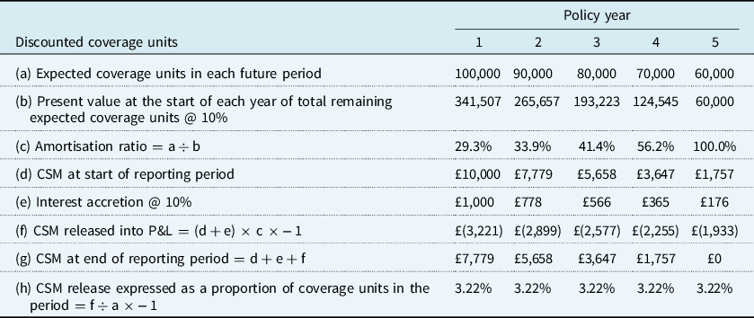
All are valued at discount rate i = 10%.
The proportions in row (h), in this case, give a constant ratio from period to period unlike the undiscounted coverage units’ scenario. This is not a coincidence: where the undiscounted scenario ends up deferring the interest unwind on the CSM for release in future years, discounting the coverage units is, in effect, akin to accelerating the release of that unwind consequently achieving the uniform release observed above.
Note that the uniformity of such a ratio does not mean that a constant ratio should in fact be locked in (or should even be expected) for the rest of the policy term; the ratio will change as actual experience emerges and as the entity updates its assumptions about the future experience.
4.6.4. Materiality of discounted versus undiscounted coverage units
Paragraph BC282 (May 2017) notes that IFRS 17 does not specify whether an entity should consider the time value of money in determining the equal allocation of the CSM remaining at the end of the reporting period to the coverage units provided in the period and the expected remaining coverage units. Indeed, it is the view of the IASB that this is a matter of judgement to be made by the entity. The materiality of this item of judgement depends on a number of factors, in particular:
-
The duration of the contract (a significantly larger impact observed on long-duration contracts).
-
The prevailing discount rate applied to assess the impact of the time value (particularly material in higher interest rate jurisdictions).
-
Certain contractual features (e.g. benefits that escalate, either at a fixed rate or in line with inflation).
Certain combinations of these three factors can result in extreme variances in the run-off of the CSM owing merely to whether the company has decided to allow for the impact of time value or not.
To illustrate this, consider a simple, profitable whole of life contract with a sum assured, which has contractual annual increases at the prevailing inflation rate, as shown in Figure 3. The contract’s premium cannot be fully reviewed (leading to a long contract boundary) and the contract is issued in an environment with a prevailing high interest (and inflation) rate.

Figure 3. Comparison of discounted annual CSM releases for a whole of life insurance contract example, both allowing and not allowing for the time value of money in nominal terms in the equal allocation of CSM to coverage units.
Using the same measure of quantity of benefits, i.e. a projection of the sum assured under the contract, escalating to allow for the annual inflation-linked growth, a company could obtain two distinct annual CSM release patterns by either allowing for or not allowing for the impact of the time value of money in nominal terms determining the equal allocation of the CSM to the coverage units. Both approaches would be allowed under IFRS 17 despite resulting in two possible extremes as shown in the graph below: the potential for excessive profit deferral when not allowing for time value and the potential for undue profit acceleration when allowing for time value. The observed difference between these extremes is exacerbated by the fact that this policy has escalating benefits and is sold in a high-interest rate environment.
Given that the Standard explicitly allows either approach (which could result in a significantly materially disparate profile of releases of CSM over time as shown above) and that paragraph BC282 (May 2017) ultimately considers this item a matter of judgement to be made by an entity, some practitioners may seek to follow an “intermediate” approach. Such an intermediate approach should best capture the entity’s view of the measurement of service. The chosen approach should be disclosed, with a robust, repeatable methodology being applied consistently over time.
One potential intermediate and pragmatic approach could see the entity not discounting the quantity of benefits in the coverage unit calculation but concurrently not modelling the annual contractual inflationary increases solely for the purposes of determining the coverage unit (i.e. it would still model these contractual increases for the fulfilment cash flows and CSM adjustments if relevant). Alternatively, an entity may allow for the impact of the time value of money in real terms in determining the equal allocation of the CSM to the coverage units. Either approach acknowledges the fact that in real terms, the company is providing the same level of cover (hence service) over time – this may prove to result in the most appropriate recognition of profit, particularly in a high-interest rate and high inflation markets where benefits may escalate over time to maintain a policyholder’s real level of cover.
The resultant impact on the CSM release of allowing for an equal allocation of the CSM to coverage units in real terms is shown in the green bars in Figure 4. The method defers the release of profits relative to the allowance for time value in nominal terms and may be considered more appropriate by the entity for a longer duration contract.
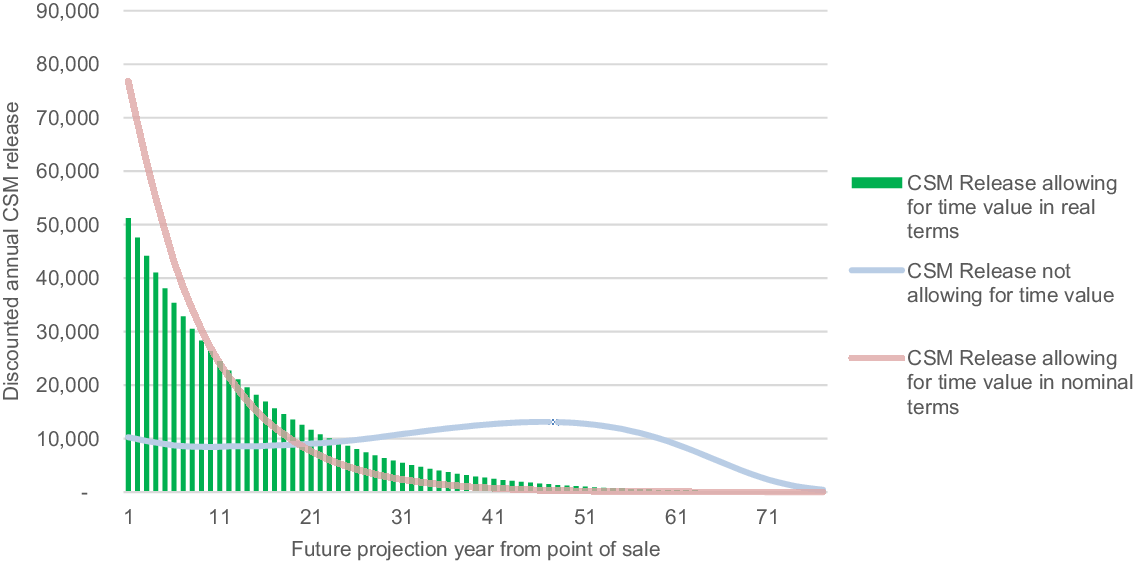
Figure 4. Discounted annual CSM release for an intermediate approach to allowing for the impact of time value of money compared to the CSM releases when explicitly both allowing and not allowing for the time value of money in nominal terms.
The above approaches are by no means exhaustive and it should be noted that there are many potential methods an entity could look to apply. The entity will, however, need to justify that the chosen approach best captures their view of measurement of service and is consequently most in line with the principle of IFRS 17.
4.6.5. Reassessment of future coverage units
The preceding sections cover possible approaches and challenges that an entity may come across whilst determining coverage units more generally. However, one topic that has not yet been addressed is the reassessment of coverage units due to changes in assumptions or experience adjustments as they occur. This section, therefore, explores angles that companies could consider in this reassessment to allow for these possibilities.
As noted, there will be two aspects relevant to the discussion here. One relates to the reassessment of coverage units expected to be provided in future periods and the other relates to the determination of coverage provided in the current reporting period. Each item is described in turn.
Reassessment of future coverage units
The long-term nature of life insurance contracts means that the entity’s estimates about the future can change as experience emerges. This means that the expected future coverage units identified in previous reporting periods can be very different from the entity’s revised expectations of the future coverage units as determined during the current reporting period (based on the latest assumptions).
Nevertheless, IFRS 17 requires that future coverage units should be reassessed at each reporting date and should be based on the latest assumptions. As part of this, non-economic assumptions pertaining to mortality, lapses, etc., will typically be intuitive enough to allow for irrespective of GMM or VFA, but the appropriateness of using the latest economic assumptions may be less obvious (e.g. should coverage units be based on locked-in financial assumptions for GMM to be consistent with the CSM estimates?).
Note, for the avoidance of doubt that any adjustments to future coverage units will apply as at the end of the current reporting period. That is, future coverage units must not be recalculated as at the start of the current reporting period as this distorts the view of coverage provided in the current period. This brings the discussion to the second relevant aspect.
Determining the number of coverage units provided in the current period
Modelling simplifications made as to the timing of decrements do not track the timing of decrements as they occur in the real world. For example, in reality, deaths do not all happen at the end or the middle of a reporting period as many models typically assume. Consequently, when determining the amount of coverage provided in the current period, an entity will need to consider whether it wishes to apply more sophisticated approaches to better reflect how much cover has been provided than suggested by the models. Note that IFRS 17 is not explicit about requirements here and so the application of judgement will become vital. Note that this does not mean that a company needs to track what is actually paid out (this is irrelevant in the context of coverage units), instead the issue is whether a company should track when claims have been paid (or incurred or reported) to better approximate the average amount of service provided over the reporting period.
Before continuing, it is important to note that consideration must be paid as to whether more sophisticated approaches are expected to have any material impact on the CSM released at all – to avoid doubt, this is an assessment that must be made at the time of setting methodology and not on an ongoing basis (companies cannot arbitrarily decide to change the approach in a year where they can get a materially better answer).
Consider a group of insurance contracts comprising of 100 policies each with a benefit payable of £1000 units. At inception, the entity expects 10 policyholders to die at the end of each year. The expected coverage units for each future year based on this initial view are shown in Table 16.
Table 16. Example of Expected Coverage Units for Future Years

Consider now what might happen if actual experience is different from expected experience after the first year (i.e. it is assumed that in year 1, actual experience is as expected but that there are experience variances in year 2). In year 2, there are 24 deaths instead of the expected 10 and that they all happen uniformly over the year (2 deaths per month). The assumption of expected deaths in the future remains unchanged, i.e. 10 per annum.
The entity now needs to decide how to reflect this experience in its determination of coverage units. It considers two possible options:
-
(a) Update its view of future coverage units from year 3 onwards to reflect the actual experience but not to update its view of the coverage units in year 2.
-
(b) Update both its view of future coverage units from year 3 onwards as well as the coverage units in year 2 (i.e. adjust the coverage units in year 2 to reflect that service stopped being provided for those policies as and when they went off the books).
These options would numerically translate as shown in Table 17.
Table 17. Example of Options when Determining Coverage Units

The premise behind option A is that the timing of deaths should not affect what could be viewed as the “absolute” amount of service that has been provided in a given period. That is, even though deaths have occurred uniformly over the year, and on average service has been provided to 78 policies (average of 90 policies at the start of the period and 66 remaining at the end of the period), service has nonetheless, in absolute terms, been provided to 90 policies as a whole in that period. Meanwhile, expectations of coverage units from year 3 onwards are adjusted to reflect that there are now fewer than expected policies remaining in the future, and consequently, the amount of service expected to be provided in the future needs to be revised downwards.
The motivation behind option B is the view that coverage units in a given period should reflect the fact that service stops being provided for those policies that go off the books (as and when they go off the books). Option B consequently sees the absolute view of Option A as typically overstating the amount of service that the company has provided over the year since it fails to take actual decrements in the period into account. Nevertheless, expectations of coverage units from year 3 onwards are adjusted in the same way as option A.
In support of option B, some companies might consider the possibility to allow for, say, the higher amount of service provided on average in a year due to unexpected increases to sums assured by policyholders (but that do not result in modification or de-recognition).
In opposition to option B, depending on the volume of business and the complexity of the product design, this approach has the risk of becoming an unmanageably complex method to track and implement and could be too complex an attempt to measure the provision of service.
In conclusion, any approach chosen by a company will need to be one that strikes a balance between practicability and accuracy.
4.6.6. Further reading
As our discussion shows, the determination of coverage units is likely to be one of the most challenging aspects of IFRS 17 implementation for many companies. Readers may find the following documents useful to consult and gain further perspectives:
-
Canadian Institute of Actuaries: Draft Educational Note – IFRS 17 Coverage Units for Life and Health Insurance Contracts
-
Singapore Actuarial Society: IFRS 17 Workgroup Resources: Coverage Units
-
Institute of Chartered Accountants in England and Wales (ICAEW): Coverage period and CSM release for deferred annuities
-
EFRAG: IFRS 17 Insurance Contracts and Release of the Contractual Service Margin: Briefing Paper
4.7. Loss Components
4.7.1. Introduction
The primary aim of this section is to draw the reader’s attention to the various possibilities that exist with respect to the systematic reversal of LC. In addition, the discussion explores the tangential issue of whether changes in fulfilment cash flows used to adjust LC should be based on current or locked-in interest rates.
First, a brief overview of LC is provided.
Then, there is a discussion about the purpose of systematically reversing LC. A strong understanding of this makes the rest of the discussion intuitively obvious and fruitful.
What follows are three possible systematic reversal methods that companies could consider as part of their LC methodology. For each method, it notes some of the obvious technical and operational consequences.
The analysis then leads into deeper, technical considerations in relation to LC systematic reversals: whether the systematic allocation ratio (SAR) can exceed 100%; whether OCI should be included in reversals; how the timing of assumption updates affects the SAR; whether insurance acquisition cash flows can be systematically allocated to the LC.
The section closes by considering whether fulfilment cash flow adjustments to LC should be based on current or locked-in interest rates.
4.7.2. Overview
For direct business written, IFRS 17 requires an asymmetric treatment of profitable and onerous groups of contracts. For profitable groups, entities are required to spread the recognition of profits (i.e. the CSM) over the lifetime of the group of contracts based on a measure of service provided. For loss-making groups, losses must be recognised in the P&L immediately via the establishment of a LC; i.e. it is not possible to set up a “negative CSM” and spread the recognition of the losses over the coverage period. However, the requirements in relation to LC do not end there; having recognised a LC, IFRS 17 then requires it to be systematically reversed such that there is a “zero” LC balance by the end of the coverage period.
Why does IFRS 17 require the systematic reversal of LC? As shall be shown, the answer is simply to prevent the recording of amounts as revenue which have not been received and to avoid the re-recording of amounts as service expenses which have already been recognised. This shall now be explained in more detail.
4.7.3. Why do entities need to systematically reverse loss components?
Consider the following question: once a P&L hit has been recognised on day 1, why does the LC balance need to be systematically reversed at all?
Here is an extract of paragraph 49:
“…The loss component determines the amounts that are presented in profit or loss as reversals of losses on onerous groups and are consequently excluded from the determination of insurance revenue.”
At first glance, this paragraph is not immediately intelligible. What are “reversals of losses”? What is the connection between LC and revenue?
Paragraph 50 continues:
“After an entity has recognised a loss…it shall allocate: …subsequent changes in fulfilment cash flows specified in paragraph 51 on a systematic basis between: i) the loss component of the liability for remaining coverage; and ii) the liability for remaining coverage, excluding the loss component.”
This paragraph fares no better for a less familiar reader. Why do certain items need to be systematically allocated to the LC? A simple example will help answer these questions.
Example 4.4. Consider a 2-year term insurance contract where:
-
An annual premium of £1 is payable at the start of each year (total premiums = £2).
-
Expected claims and expenses of £30 and £70 are paid at the end of each year, respectively, (total outflows = £100).
-
The RA and the impact of discounting are negligible so can be ignored.
-
Actual experience is exactly in line with that expected.
This gives the fulfilment cash flows as shown in Table 18.
Table 18. Example of Fulfilment Cash Flows for a 2-Year Term Insurance Contract

As one would expect, the contract is identified by the entity as onerous at initial recognition and a LC balance of £98 is established.
Consider now how the insurance service result (i.e. the P&L statement) might be populated for such a contract if systematic reversals of LC did not exist. This example is shown in Table 19.
Table 19. Example of Insurance Service Result if Systematic Reversals of Loss Components did not exist
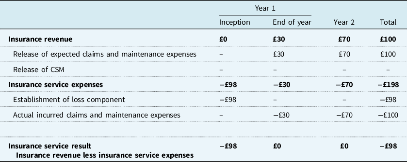
Observations about Example 4.4
-
At initial recognition, the entity records a £98 loss in the P&L via the establishment of the LC.
-
Once the day 1 loss is recognised, zero profits/losses are reported in subsequent years and this is also consistent with expectations.
-
The total insurance service result at the end of 2 years shows a loss of £98 and is in line with what one would expect it to be.
-
This was all achieved without having to worry about systematically reversing the LC and considering any of the systematic allocation requirements of IFRS 17.
If that is all that is the case, why does IFRS 17 have so much to say about LC?
Problems that arise from Example 4.4
There are two fundamental problems with the results presented here:
-
(1) The total reported insurance revenue over the 2 years is £100. This does not make sense. How can the total revenue be £100 when the company only received total premiums of just £2? Not only is this difficult to make sense of, this also contradicts the requirements of paragraphs 83, B120 and B123.
-
(2) The total reported insurance service expenses over the 2 years is £198. This does not make sense either. How can the total insurance service expense be £198 when the company only incurred total actual claims and maintenance expenses of £100? This also contradicts the definition of insurance service expenses as per paragraph 103.
The incoherence of the results produced here suggests that something is missing – there must be some way of reflecting that revenue cannot be higher than the premiums received, and the service expenses cannot be higher than the actual outflows.
Indeed, there is such a way.
Example 4.5 Working with the same onerous contract from Example 4.4, consider now how the P&L statement should be populated, in line with the IFRS 17 requirements, by systematically reversing LC. This example is shown in Table 20.
Table 20. Example of Profit and Loss Statement when Systematically Reversing Loss Components

Before proceeding, note that the systematic allocation method used in this example does not matter yet: this will be discussed in exhaustive detail in 4.7.4. For now, the reader’s aim should simply be to understand why a method is required in the first place.
Calculation notes
It should first be noted that the SAR is being recalculated at the start of each reporting period.
The ratio is being calculated by applying an extremely simplified version of a method shown in IFRS 17 Illustrative Example 8.
Consequently, in this example, the SAR to apply for year 1 is calculated as
 $${{{\rm{loss}}\;{\rm{component}}\;{\rm{at}}\;{\rm{beginning}}\;{\rm{of}}\;{\rm{year}}\;1} \over {{\rm{PV}}\;{\rm{expected}}\;{\rm{claims}}/{\rm{expenses}}\;{\rm{at}}\;{\rm{start}}\;{\rm{of}}\;{\rm{year}}\;1}} = \;{{\pounds 98} \over {\pounds 100}} = 98\% = {\rm{year}}\;1\;{\rm{SAR}}.$$
Similarly, the SAR to apply for year 2 is calculated as
 $${{{\rm{loss}}\;{\rm{component}}\;{\rm{at}}\;{\rm{beginning}}\;{\rm{of}}\;{\rm{year}}\;2} \over {{\rm{PV}}\;{\rm{expected}}\;{\rm{claims}}/{\rm{expenses}}\;{\rm{at}}\;{\rm{start}}\;{\rm{of}}\;{\rm{year}}\;2}} = \;{{\pounds 68.6} \over {\pounds 70}} = 98\% = {\rm{year}}\;2\;{\rm{SAR}}.$$
-
(a) The amounts in row 3 have been calculated by applying the SAR applicable in that year to the release of the expected claims and maintenance expenses in revenue that year. For example:
-
£29.4 = £30 (amount released in revenue) × 98% (year 1 SAR),
-
£68.6 = £70 (amount released in revenue) × 98% (year 2 SAR).
-
-
(b) The amounts in row 7 are equal and opposite of the items in row 3.
-
(c) The amounts in row 10 are calculated as cumulative balances of the establishment of the LC and the subsequent reversals. For example, by the end of year 1, the LC balance of £68.6 is calculated as the starting LC of £98 less the £29.4 amount reversed or amortised over the year.
Observations about Example 4.5
Compared to the results in Example 4.4, the results in Example 4.5 look much more reasonable:
-
The total reported insurance revenue is £2 and is now exactly equal to the consideration/premiums received over the lifetime of the contract. This meets the requirements of paragraphs 83, B120 and B123.
-
The total reported insurance service expense is £100 and is now exactly equal to the actual claims and expenses incurred over the lifetime of the contract. This meets the definition in paragraph 103.
-
The establishment of the LC in row 6 (i.e. −£98) and the subsequent reversals of the LC in row 7 (i.e. £68.6 + £29.4 = +£98) net off fully to equal zero by the end of the contract. This meets the requirement of paragraph 52.
More importantly, Example 4.5 also provides a deep insight into the nature of the SAR and the reversals of the LC:
-
The systematic allocation has the impact of reducing both the insurance revenue and insurance service expenses in a period. For example, in year 1, revenue was reduced from £30 in Example 4.4 to just £0.6 in Example 4.5. Similarly, in year 2, service expenses were reduced from £70 in Example 4.4 to £1.4 in Example 4.5. This meets the requirements of paragraph 49.
-
The amount by which revenue is reduced is directly dependent on the LC (at this point it is strongly recommended the reader refers to the extract of paragraph 49 included in section 4.7.3). In this example, the SAR was 98% in both years. This means that only 2% of the premium received was sufficient to cover the outgo. Consequently, the reported revenue should only be 2% of the unadjusted revenue items that would have been released otherwise (i.e. the unadjusted release of claims and maintenance expenses in revenue).
-
The impact of systematically allocating items to reverse/amortise of the LC has no bottom-line impact on the insurance service result in a given reported period; items that are excluded from revenue are simultaneously excluded from the service expenses to give a net impact of zero.
Summary
Several questions were raised throughout this discussion. These can now be answered.
-
Why does the LC need to be systematically reversed? The systematic reversal of LCis what enables the insurance service result (i.e. the P&L statement) to be populated in a sensible manner. If LC were not amortised, both insurance revenue and insurance service expenses would be overstated (compare Examples 4.4 and 4.5). The systematic reversal is effectively what “fixes” this overstatement issue.
-
What is the connection between LC and insurance revenue? The systematic reversal of LC requires a systematic allocation of certain items that are released in the insurance revenue line in a reporting period. Systematically allocating these items has the dual purpose of reducing the revenue (i.e. “fixing” it for the overstatement problem) and systematically reversing the LC.
The rest of the discussion can now build on this foundation and attempt to answer the next logical question: how should the LC be systematically reversed?
4.7.4. How should loss components be systematically reversed?
The Standard sets out some basic requirements when it comes to systematically reversing LC. However, beyond this, IFRS 17 does not ultimately prescribe an approach. What are these requirements?
Paragraph 50 requires that the LC be reversed on a systematic basis. In other words, entities cannot reverse LC by arbitrary amounts of their choosing; there must be a systematic, formulaic approach by which this must happen. But what must the components of that formula be?
Paragraph 51 states that the systematic reversal must have a connection with certain items that will be recognised in the P&L in a given reporting period. Namely: the release of the expected claims, expenses and RA in the insurance revenue line, as well as amounts released in the insurance finance income and expenses line. For the rest of this section, these items (to be systematically allocated) will collectively be referred to as “allocatables”.
How will these requirements be applied in practice? This section will consider three possible methods. Each method is, to the Working Party’s belief, technically compliant as these are “systematic” approaches that avoid arbitrariness.
Example 4.6 – Method used in IFRS 17 Illustrative Example 8
This example is a slight variation of the example used in the previous section. Here:
-
An annual premium of £1 is payable at the start of each year (total premiums = £2).
-
Expected claims of £30 and £50 are paid at the end of each year, respectively, (total claims = £80).
-
Expected expenses of £8 are incurred at the end of each year (total expenses = £16).
-
The RA at inception is £4 (released evenly each year).
-
Interest rates are 0%.
-
Actual experience is exactly in line with that expected.
This gives the fulfilment cash flows at initial recognition and subsequent measurement as shown in Table 21.
Table 21. Example of Fulfilment Cash Flows at Initial Recognition in line with Method used in IFRS 17 Illustrative Example 8

The contract is onerous at initial recognition and consequently, the entity will establish a LC and recognise a loss in the P&L of £98.
How should this LC be systematically reversed?
Based on the method used in IFRS 17 Illustrative Example 8, the formula used to determine the SAR to systematically reverse the LC will be:
 $$\rm {SAR = \;{{loss\;component\;at\;the\;beginning\;of\;the\;reporting\;period} \over {PV\;of\;cash\;outflows + risk\;adjustment\;balance}}$$
This can then be used to complete the required computations as shown in Tables 22 and 23.
Table 22. Example of Systematic Allocation Ratio Calculation

Table 23. Example of Opening and Closing Loss Component Calculation

Observations about Example 4.6
-
It is not a coincidence that the SAR in years 1 and 2 is 98%. In the absence of any assumption updates or experience variances relating to future service, this method results in a stable proportion of future allocatables being systematically allocated to the LC. However, in the real world, the fact that assumption updates or experience variances relating to future service are virtually guaranteed to occur means that it will be almost impossible for the SAR to be the same from period to period for the same group of contracts.
-
On a practical note, this method will require additional calculations to determine the SAR. Whilst these ratios do not need to be stored for future use, the fact that they need to be recalculated at each reporting period and then applied to the allocatables means that this is a computationally intensive process.
-
Whilst for GMM contracts it might be easier (but not easy) to identify the PV of cash outflows separately from the PV of cash inflows, for VFA contracts (like UL business), cash outflows like investment expenses may be implicit (i.e. netted off) as part of the AMC projections and not necessarily modelled separately. It is important to note that NDIC must not be included as part of the cash outflows (as they do not form part of revenue) which means that the computations will become much more difficult.
-
There are divergent opinions on whether the PV of cash outflows (for the denominator of the SAR) must be measured at locked-in rates or current interest rates for GMM contracts. Both methods are possible and can be demonstrated to meet the requirements of the Standard. This point will be discussed in section 4.7.6 (albeit in a slightly different context).
Example 4.7 – Set the SAR to 100% as default
This example uses the same contract from Example 4.6. Under this method, instead of (re)calculating the SAR based on the formula described in Example 4.6, the entity could simply allocate 100% of the allocatables to the LC. In a reporting period where 100% of the sum of the allocatables is higher than the residual LC, the method falls back to the method in Example 4.6 to avoid creating a CSM. The related calculations for this example are shown in Tables 24 and 25.
Table 24. Example of Setting the Systematic Allocation Ratio to 100% in the First Year

Table 25. Example of Opening and Closing Loss Component Calculation using a Systematic Allocation Ratio of 100% in the First Year

Observations about Example 4.7
-
It systematically reverses the LC as quickly as possible and consequently increases the likelihood of a CSM being established (subject, of course, to future favourable assumption updates or experience variances relating to future service). There are differing views in the Working Party as to whether this is commercially desirable or not: slowing down the systematic reversal of the LC means that favourable basis updates can be recognised immediately (and more often) without having to set up a CSM (which results in a deferral of recognition of those profits). On the other hand, the CSM reduces P&L volatility which could be more desirable.
-
Operationally, this is a less computationally intensive and an easier to follow calculation – however it does not avoid complexity entirely as it will still be necessary to apply the method in Example 4.6 at some point in coverage period of the group of contracts.
-
The key disadvantage of this approach is that it results in the smallest amount of revenue in a given reporting period compared to all other methods. Specifically, revenue in a given period will be equal to the amount released for insurance acquisition cash flows relating to that group of contracts. If the insurance acquisition cash flows are zero or small, then the revenue reported is zero or close to zero. This is an important consideration for developing future KPIs.
Example 4.8 – Set the SAR to be equal to the CSM amortisation ratio
This example uses the same contract from Example 4.6. In this context, the CSM amortisation ratio simply means the ratio determined by coverage units. The fact that a LC cannot exist simultaneously with a CSM for the same group of contracts is irrelevant as coverage units can be determined without a CSM.
Under this method, the SAR will be set to be equal to the CSM amortisation ratio.
Like Example 4.7, in a reporting period where the 100% of the sum of the allocatables is higher than the residual LC, this method will also need to fall back to the method in Example 4.6 to avoid creating a CSM. The related calculations for this example are shown in Tables 26 and 27.
Table 26. Example of Setting the Systematic Allocation Ratio to be equal to the CSM Amortisation Ratio

Table 27. Example of Opening and Closing Loss Component using a Systematic Allocation Ratio equal to the CSM Amortisation Ratio

However, there is one peculiarity that emerges in this method that was not possible in the previous two.
Assume the CSM amortisation ratios and SAR are determined to be as shown in Table 26.
Observations about Example 4.8
-
This is an operational simplification as it might be that the entity amortises the insurance acquisition cash flow balances with the same ratio as well.
-
As with Example 4.7, this is less computationally intensive and an easier to follow calculation – noting again that it does not avoid complexity entirely as it will still be necessary to apply the method in Example 4.6 at some point in coverage period of the group of contracts.
-
In the reporting period where the SAR is greater than 100%, this could result in “negative” revenue. However, as noted above, this possibility is not unique to this method rather it is just made more obvious. This is also an important consideration for developing future KPIs. Section 4.7.5 considers whether or not the SAR can be greater than 100%.
Conclusions
-
Whilst many companies will find it tempting to use the method used in IFRS 17 Illustrative Example 8, this paper has attempted to show that many other practical and sensible methods are available that should be carefully considered before being rejected. The preceding discussion has explored three such possible methods though there may be others.
-
The LC balance at transition does not affect companies’ shareholder equity. However, companies will need to weigh up the pros and cons on whether to select a systematic reversal methodology that maximises or minimises the LC balance at transition:
-
○ Minimising the LC balance at transition will maximise the likelihood of being able to reverse these balances out entirely and recognising CSMs after transition (if favourable updates occur). This could be desirable because of the “stabilising” nature of the CSM and the ability to spread and recognise a stream of profits in the future.
-
○ On the other hand, maximising the LC balance at transition might be deemed more acceptable as favourable basis updates can be recognised immediately in full without having to set up a CSM and defer their recognition.
-
The discussion now proceeds to reflect on some deeper considerations in relation to LC.
4.7.5. Deeper considerations
Can the SAR be greater than 100%?
This question arose from Example 4.8.
The simple answer is yes, it is entirely possible for the SAR to be greater than 100% in all possible approaches – Example 4.8 is not unique in this regard.
The detailed answer is that there are two possible scenarios under which the SAR can be greater than 100%.
Scenario 1: “Less than optimum ratios”
This scenario arises when an approach used to determine the SAR consistently results in a ratio that is lower than its “optimum”.
Note that the usage of the term optimum simply means the ratio based on the formula described in Example 4.6 (i.e. based on IFRS 17 Illustrative Example 8) – the usage is not intended in the sense of a ratio that optimises technical/operational/financial consequences (as that is a matter for an entity to conclude based on their specific circumstances).
This description explains why Example 4.8, and not Examples 4.6 and 4.7, resulted in a SAR greater than 100%.
In Example 4.8, there was a SAR of 130% in the final year as it did not amortise the LC in the first year by the “optimum” rate of 98%.
By contract, Example 4.7 will consistently result in a ratio that will be higher than the optimum (as it usually always set to be 100%) and so there is no possibility for this scenario to arise here.
Example 4.6 by definition, applies the “optimum” ratio for all periods and consequently, the possibility for this scenario does not arise here either.
But if this is true, under what circumstances might Example 4.6 or Example 4.7 result in a SAR greater than 100% (given that they both amortise the LC at or above the optimum)?
This brings the discussion to the second possible scenario.
Scenario 2: Experience variances relating to future service
It is theoretically possible, though with low probability, for there to be an experience variance relating to future service that adjusts the LC without affecting the PV of outflows or the RA.
Premium and acquisition expense variances are two such eligible items that can cause the LC to be greater than the PV of the outflows and the RA; this can result in a SAR greater than 100%.
Summary
Table 28 summarises which scenarios can apply for the three methods that were explored in this section.
Table 28. Summary of Systematic Allocation Ratio Methods Considered and its Usage in each Scenario

Should OCI be systematically allocated to the loss component?
Note that this question is relevant to, and recommended to be read in conjunction with, the discussion in section 4.7.6.
Paragraph 51 identifies “insurance finance income or expenses” as an item that must be systematically allocated to the LC. However, it identifies this in the context of the subsequent changes in fulfilment cash flows.
If an entity applies the OCI disaggregation approach for a portfolio of GMM contracts, must it systematically allocate the OCI to the LC?
There are three considerations.
First, it is only the OCI arising on the PV of cash outflows that can be allowed here. Allowing for the full OCI (including that arising on the PV of cash inflows) will not allow the LC to be amortised to zero at the end of the coverage period – thus falling foul of IFRS 17 requirements. This means that operationally, entities will need to be able to identify the PV of cash outflows separately from the PV of cash inflows.
Second, systematically allocating the liability OCI to the LC will result in an accounting mismatch compared to the asset OCI. In the most straightforward example, take a perfectly matched asset/liability position and assume that the asset OCI arising in a period is 100 (and so it is known that the liability OCI arising will also be 100). If, say, 5 of the liability OCI is allocated to the LC, then the entity will have an OCI mismatch arising in equity: 95 liability OCI compared to 100-asset OCI.
Third, under Example 4.6, it was observed that the SAR was constant. Even if Example 4.6 were extended to allow for interest rates, it is possible for the SAR to remain constant by not allocating the OCI to the LC. In other words, allocating the OCI to the LC has a destabilising effect. This is potentially not a major problem given that the SAR will change every reporting period anyway.
Ultimately, companies must form their own opinions as to the considerations raised here.
Should the insurance acquisition cash flows be systematically allocated to the LC?
Whilst it is entirely possible to do so mathematically speaking, this is strictly speaking not in compliance with the Standard and consequently not explored in this section further.
IFRS 17 makes it clear that it expects to see the full value of the proportion of premiums that relate to the recovery of insurance acquisition cash flows – this requirement is not met if insurance acquisition cash flows are systematically allocated to the LC.
How does the timing of assumption updates affect the SAR?
From a practical point of view, the method described in Example 4.6 is necessarily simplistic and does not reflect that entities will perform assumption updates at regular intervals.
To address this, one possible modification to the formula applied might be as follows:
 $$\rm{SAR = {{adjusted\;oeing\;loss\;component\;} \over {revised\;PV\;of\;cash\;outflows\; + revised\;risk\;adjustment\;balance}}}$$
Here:
-
The adjusted opening LC refers to the LC after the assumption updates have been performed.
-
The revised PV of cash outflows and RA balance reflects the fact that the view of future cash flows and the corresponding uncertainty will have changed because of the assumption updates.
-
The ratio is not retrospectively applied from the start of the reporting year, rather only from the point at which the updates are applied. For example, if the assumption updates were applied as of 30 June of a financial year running from 1 January to 31 December, then the SAR determined as of 30 June would only apply for cash flows arising between 1 July and 31 December and not retrospectively applied to cash flows between 1 January and 30 June.
The order in which the allocation is performed should be considered consistent with the order in which adjustments to the CSM are made (click here).
For completion, it is separately noted the actual impact of the assumption updates will affect the LC and the P&L as follows:
-
Unfavourable assumption changes will increase the LC and be recognised in the P&L as an immediate hit (through an “increase to the loss component” line in insurance service expenses).
-
Favourable assumption changes will decrease the LC and be recognised in the P&L as an immediate gain (through the “reversal of loss component” line in insurance service expenses). Note, however, that if the size of the gain is larger than the LC, then the P&L gain recognised is capped to the value of the LC that has now been extinguished. Any “excess” left behind is used to establish a CSM which will then be recognised over the lifetime of the group of contracts (as per the usual requirements).
Conclusions
-
There are several technical complications that companies must consider during implementation. Methods should be carefully considered in terms of what financial and operational implications it commits entities to – considerations for in-force business may result in completely different conclusions compared to considerations for new business. Ultimately, a balance will need to be struck.
-
The SAR can be greater than 100%. There are two scenarios where this is made possible. One relies on the concept of “optimum” ratios, the other on the theoretical possibility of there being experience variances relating to future services that do not affect the view of future cash outflows or the RA.
-
Systematically allocating OCI to the LC is possible but comes at a price of potential accounting mismatches.
-
Assumption updates can complicate the specific formulation of SAR as can technical choices about whether to use PV of cash outflows at locked-in or current interest rates.
4.7.6. Should changes in fulfilment cash flows, which are solely allocated to the loss component, be calculated using current or locked-in interest rates under the GMM?
Overview
When it comes to the GMM, the Standard is explicit in requiring the use of locked-in discount rates for subsequent adjustments to the CSM (see paragraph B96(b)). However, there is a wider debate whether this requirement also holds in respect of the LC. This section explores the issue and considers whether changes in fulfilment cash flows, that need to be solely allocated to the LC, ought to be based on locked-in or current interest rates.
Analysis of the two positions
An insurer could adopt any one of the two positions in respect of this question:
-
(1) The LC balance must be adjusted by changes in fulfilment cash flows on locked-in interest rates. Under the GMM, changes in discount rates do not affect the CSM because they do not relate to future service and the LC treatment ought to be consistent with the CSM.
-
(2) The LC balance must be adjusted by changes in fulfilment cash flows on current interest rates.
There are pros and cons of choosing each option. For example, an advantage of the locked-in basis is that there is no need to set out a justification for the choice of locked-in rates that would be used should a CSM be re-established. In this case, locked-in interest rates that have been used since the contract inception for tracking the LC will continue to be used for the CSM.
On the other hand, companies that use current interest rates for tracking the LC could argue that this paints a more realistic picture of the development of the LC as it takes current interest rates into account.
In either case, the way the LC is tracked, adjusted and reduced to zero by the end of the coverage period will need to be clearly specified in the methodology used by the company. Each route has operational implications.
Worked examples
The examples below in Tables 29 and 30 show the tracking of a LC, including adjustment for changes in fulfilment cash flows, under both methods on a 3-year policy. The only change since the policy inception is a change in interest rates from initially assumed 5% to a reviewed basis of 3% at the start of year 2. For both scenarios, consider:
-
A 3-year policy.
-
Single premium: £10,000.
-
Claims at the end of each year: year 1 = £1,000; year 2 = £1,000; year 3 = £10,000.
-
Discount rate at initial recognition: 5%.
-
LC at initial recognition: £498.
-
At the start of year 2, assumptions are reviewed, and discount rates are set to 3% going forward.
-
The SAR used in this example is
 $$\rm{SAR = \;{{loss\;component\;at\;the\;beginning\;of\;the\;reporting\;period} \over {PV\;of\;cash\;outflows\;at\;the\;beginning\;of\;the\;reporting\;period}}.$$
-
(1) To be consistent with the measurement of the CSM, the company measures the LC assuming a locked-in discount rate of 5%. Consequently, the unwind of the discount rate is based on 5% throughout the lifetime of the contract. Note for completion that the PV of claims that appears on the balance sheet will be based on the current interest rates in line with the Standard’s requirements.
-
(2) It follows from (1) that since changes in discount rates do not adjust the CSM under GMM, they will not adjust the LC under GMM either. Consequently, the change in discount rates at the start of year 2 has no impact on the LC. Instead, this impact will be recognised through the P&L (or OCI) when it happens.
-
(3) Unlike scenario A, the SAR changes to reflect the view that the relevant PV of claims to consider is that measured at current rates instead of locked-in rates.
-
(4) The impact on the PV of claims, at the start of year 2, from the change in discount rates is 374 = PV of claims @ 3% of 10,397 (see scenario B) – PV of claims @ 5% of 10,023 (see scenario B). Consequently, the amount allocated to the LC due to changes in the discount rate is = 374 × 4.57% = 17.
Table 29. Scenario A: changes in Fulfilment Cash Flows Measured at Locked-in Rates

Table 30. Scenario B: changes in Fulfilment Cash Flows Measured at Current Rates

Conclusion
There is no straightforward answer to this question and views are strongly held on both sides of the camp even within the Working Party. It is noted that many companies have already built their systems to reflect their preferred positions which means that this could be an ongoing source of difference when comparing results.
Further reading
For an especially useful and detailed survey of the various interpretations in this space, see:
-
Paper 3 of the Hong Kong Insurance Implementation Support Group (HKIISG):
-
….and the corresponding meeting summary notes:
4.8. Reinsurance Contracts Held
4.8.1. Setting consistent assumptions
This section discusses the consistency requirement between assumptions used for the valuation of reinsurance contracts held and the underlying insurance contracts as per paragraph 63.
It is noted that the requirement may result in different interpretations. Largely the view is that the consistency requirement does not mean the assumptions have to be the same, but rather the differences, if any, need to be clearly justified. This has important consequences since assumptions directly affect cash flow projections and hence the CSM.
The consistency requirement will be applicable to the assumptions used to derive the best estimate cash flow projections and discount rates for measuring reinsurance contracts on initial recognition as set out in paragraphs 32–36 through the reference from paragraph 63. Consistent does not necessarily mean the same. But where is the fine line between assumptions still being consistent and becoming inconsistent? This is clearly an area of judgement requiring justifications.
Further consistency and justification of changes will be required in subsequent measurements. It would be a natural expectation to adjust and/or reset assumptions going forward in line with experience and/or market movements. If these parameters turn out to be different and diverge over time between the ones applicable to a group of insurance contracts and the ones that are applicable for corresponding reinsurance treaties, these differences and divergence should be appropriately documented and justified. An additional P&L mismatch within a combined statement may occur in cases where assumptions are not consistent between reinsurance contracts held and their corresponding underlying insurance contracts.
The two simple examples below show examples of selected assumption consistency between reinsurance contracts held and underlying insurance contracts.
Example 4.9 – Mortality assumptions
The underlying insurance contract assumes mortality follows 65% AXC00 mortality tables. Reinsurance contract premiums to be paid under the treaty are set based on a separate age-dependent rates table provided by the reinsurer.
If the firm believes the mortality table used for the underlying insurance contracts is the best estimate of the future mortality experience for this block of business, these same rates should be taken as a base for determining reinsurance recovery cash flows under the reinsurance treaty.
IFRS 17 requires reinsurance contract fulfilment cash flows to allow for the risk of non-performance by the reinsurer.
There are various ways to allow for the non-performance risk, with the most common probably as an explicit reserve. However, one approach could be to adjust the resulting recovery cash flows for the risk of non-performance by the reinsurer. This could be achieved by adjusting the Mortality assumption with the resulting proportion being, say, 64.5% of AXC00 mortality tables though this method is less preferable and results in loss of distinguishability between variances due to mortality and reinsurer default.
The above example starts with the same mortality assumption for the insurance and reinsurance agreements, but the assumption used for the reinsurance agreement is adjusted for the risk of non-performance by the reinsurer. Documentation of this adjustment would serve as an explanation of the differences in the assumption and justification. Consistency of these two mortality assumptions will still be in place.
Example 4.10 – Discount rate assumptions
The underlying term assurance group of contracts has a risk-free discount rates curve at initial recognition. (The liquidity premium is set to zero due to the contracts being able to lapse any time.) The discount rates curve is set as a simple average of discount rates at the inception date of each contract within the group over the cohort year.
At a later date, quota share reinsurance contract was taken out to manage the mortality risk of this business. The reinsurance contract just covers the in-force term assurance business
The discount rates at the inception of this reinsurance contract held have been set as the risk-free discount rates available at the start date of the reinsurance coverage.
In this example, the underlying groups of term assurance contracts will most certainly have different discount rate curves from the discount rate curve by the value derived for the corresponding reinsurance held contract. However, the methodology used to derive the discount rate curves for the insurance and corresponding reinsurance contracts is consistent (i.e. based on the risk-free curve at recognition of the contract(s)).
The examples above are by no means intended to be exhaustive and conclusive. Neither do these examples intend to be appropriate for any firm’s actual contract groups. Many other examples exist that would satisfy the consistency requirement.
4.8.2. Recognition date and contract boundaries
This section looks at some of the challenges for reinsurance contracts held with respect to the inclusion of future ceded new business within the contract boundary and the implications on when reinsurance should be recognised on the balance sheet. The view provided within this section is from an insurer’s perspective, and hence reinsurance is held. However, many of the points discussed also apply to reinsurance contracts issued.
IFRS 17 states that all cash flows within the contract boundary that “arise from substantive rights and obligations” must be included in the fulfilment cash flows. Footnote 14 It is common for reinsurance treaties to include a notice period to make a change, applying to both parties of the treaties. Changes covered by such a notice period may include:
-
stopping future new business from being ceded to or accepted for reinsurance;
-
changes to the reinsurance premiums payable on reinsurance of future new business.
Note that such a notice period creates a substantive obligation for the insurer to cede its future new business whilst the notice period is being served. Therefore, reinsurance cash flows relating to new business the insurer expects to write during the notice period could be inside the reinsurance contract boundary under IFRS 17. This implication of the contract boundary requirements on reinsurance was discussed and acknowledged at the February 2018 TRG.
What period of future new business, if any, needs to be included in the contract boundary depends on the recognition date of the reinsurance contract and its notice period. This will be discussed later in this section. Initially, a simple example will be considered to demonstrate the principle of including future new business in the reinsurance contract boundary.
Example 4.11 An insurer has just launched a term assurance product. At the following reporting date (e.g. 31 December), it has not yet written any contracts, however, it expects to write one-term assurance contract each month going forward. It anticipates this business will be profitable. On the reporting date (i.e. 31 December), the insurer enters into a reinsurance treaty to reinsure all of the new term assurance contracts it writes. The reinsurance treaty has a 3-month notice period if the insurer wishes to stop ceding future new business.
Under IFRS 17, the underlying term assurance contracts will be recognised on the balance sheet as and when each contract is written. As a result, there will currently be no term assurance contract liabilities appearing on the balance sheet.
It is assumed here that the reinsurance contract is recognised on the reporting date. Due to the notice period, the contract boundary for this reinsurance contract held will include the reinsurance cash flows relating to the following 3 months of new business, i.e. the future reinsurance premiums, reinsurance recoveries and related expenses in respect of the three contracts it expects to write over that period. Note again that the issue at hand here relates to the contract boundary for the future new business to be covered under the reinsurance contract – this will be different to the contract boundary of the cashflows for the three contracts that are already written and covered by this reinsurance agreement (and in this case, the contract boundaries between reinsurance held and the underlying contracts need to be consistent).
In addition to resulting in accounting mismatches on the balance sheet, this requirement can also lead to the following challenges for insurers:
-
Operational complexities
Including future new business in the contract boundaries is likely to result in a number of operational complexities, not least due to the need to determine assumptions for the volume and mix of the future new business. There is an open question on how sophisticated such approaches need to be.
-
Disclosure of commercially sensitive information
By including assumptions for the volume and mix of future new business in the reported accounts, an entity risks disclosing commercially sensitive information. How easy it would be for competitors to determine such information from the accounts will depend on the nature of the business and the granularity of grouping and disclosure of results. In this example, where the insurer has launched a new product line, it could be relatively straightforward to identify their future business plans from IFRS 17 disclosures. However, for a mature book of business, this risk would be lower.
Implications for reinsurance recognition date
Notice periods on reinsurance treaties are generally of a rolling nature, e.g. a 3-month notice period can be served by either party at any time to stop the future new business from being ceded. However, at TRG in September 2018, it was clarified that the contract boundary created by the substantive obligations arising from such a notice period will be fixed from the date the reinsurance treaty is recognised. This has two consequences:
-
(1) As alluded to above, the future new business to be included in the contract boundary is a factor of both the notice period and the recognition date of the reinsurance contract. The future new business to be included in the contract boundary is that expected to be written in the outstanding period from the reporting date to the end of the notice period fixed from the date of recognition.
-
(2) Business ceded beyond this fixed contract boundary will form a new reinsurance contract on the IFRS 17 balance sheet, with a new recognition date and potentially in a different group of contracts, e.g. if the new recognition date is more than 1 year apart from contracts in the original group of contracts.
Example 4.12 Using our example above, assume the insurer enters into the reinsurance treaty on 31 December 2022. (Note – as will be shown later in this section, the exact date of recognition of the reinsurance contract is critical to the contract boundary conclusions). At that point, it assesses the treaty and determines that it should recognise a reinsurance contract (referred to as “r1”) on the IFRS 17 balance sheet as follows:
-
(a) Initial recognition date of 31 December 2022.
-
(b) The 3-month notice period implies a contract boundary that includes future new business up to and including 30 March 2023.
-
(c) r1 is included in a group of reinsurance contracts held that are referred to as “R2022”.Footnote 15
The insurer does quarterly reporting. On 31 March 2023, it remeasures the previously recognised reinsurance contract, r1. Since December, the insurer has written four-term assurance contracts. Reinsurance of these four contracts will be included in r1, replacing in the fulfilment cash flows for the three underlying contracts it estimated at initial recognition. The original contract boundary has now expired, and hence no future ceded new business under the reinsurance treaty should be included in r1. The insurer did not issue a notice to the reinsurer on 31 December, hence there is a future expected new business to be ceded under the treaty. The insurer will, therefore, recognise a new reinsurance contract, “r2”, as follows:
-
(a) Initial recognition date of 31 March 2023.
-
(b) The 3-month notice period implies a contract boundary that includes future new business up to and including 29 June 2023.
-
(c) r2 is included in the group of reinsurance contracts held that are referred to as “R2023”.
Going forward, the insurer will recognise a new reinsurance contract every 3 months; at initial recognition, each new contract will contain the following 3 months of new business. Whether the new contract falls into a new group will depend on whether it falls into a new cohort year or not.
On first reading, the TRG interpretation above seems at odds with the economics of a rolling notice period.Footnote 16
Consider the example above but assume the reinsurance treaty was entered on 30 November 2022. The contract is subsequently measured at the first reporting date after this, i.e. 31 December 2022. At this point, the contract boundary would only include future new business up to and including 27 February 2023, despite the insurer knowing that, as notice has not been given, they must cede new business up to and including 30 March.
This argument can be followed through to consider the situation where the reinsurance treaty was written on 1 October 2022, where the contract boundary will include future new business up to and including 31 December. When the insurer measures the reinsurance contract held on 31 December, they do not need to include any future new business in the contract boundary, however, neither do they need to recognise a new reinsurance contract yet.
Therefore, it could be possible to resolve the challenges identified in Example 4.11 above, by synchronising the dates on which reinsurance treaty notice periods expire with reporting dates.
There are some points to consider making this work:
-
Does the wording of existing reinsurance treaties, particularly with respect to notice period clauses, need to be amended to achieve synchronisation? Depending on a company’s transition approach, this may be deemed to be unnecessary (e.g. if applying Fair Value Approach), or simplifications to avoid its need may be justifiable.
-
For future treaties, how can the notice period and/or treaty start dates be structured to achieve synchronisation without restricting commercial activity? It is worth starting discussions with the internal teams and reinsurers early to find a workable solution.
-
For synchronisation to work, notice periods will need to be based on calendar months rather than the number of days, e.g. 3 months rather than 90 days.
As well as the opportunity to explore synchronising notice periods and reporting dates, the above interpretation of fixed contract boundaries has other advantages. In particular, this results in multiple reinsurance contracts being recognised with different recognition dates within a single reinsurance treaty. This reduces the degree of mismatch between underlying insurance contracts and reinsurance contracts held in areas such as discount rates.
Conclusion
In summary, the treatment of future new business under reinsurance contracts has been clarified by discussions at TRG meetings. Whilst the interpretation arguably does not represent the economics of reinsurance notice periods, it offers opportunities for insurers to explore that may help mitigate some of the challenges arising if the future new business is included in the reinsurance contract boundary.
Further reading
For an excellent guide that considers further nuances of contract boundaries under IFRS 17, see:
-
Hong Kong Institute of Certified Public Accounts: Pocket Summary – Implementing HKFRS/IFRS 17 Contract Boundary
4.8.3. Aggregation
This section explores how reinsurance contracts held could be aggregated into groups of contracts under IFRS 17. There are several considerations here. Unlike (re)insurance contracts issued, reinsurance contracts held can have a positive or negative CSM. Further, underlying business written may in practice be covered by more than one reinsurance contract. In some instances, a single complex reinsurance programme may be structured through a combination of basic reinsurance arrangements. What are the implications of the level of aggregation requirements on how these considerations interact? This question is discussed below supplemented with some examples.
Aggregation of contracts, i.e. grouping, impacts the size of the CSM in each group and its behaviour. Each contract, by its size, coverage structure and expected profitability will be adding its own contribution to the CSM in terms of the present value of expected profits and CSM release pattern. Therefore, the behaviour of the CSM for a group of contracts will directly depend on the contracts aggregated within the group.
In the context of IFRS 17’s level of aggregation requirements, reinsurance contracts issued are treated in the same way as insurance contracts issued (refer to paragraphs 3 and 4 of IFRS 17), but different requirements apply to reinsurance contracts held. For reinsurance contracts held, paragraphs 60–70 apply and according to this, reinsurance contracts held would be aggregated in the following three profitability groups:
-
(a) Groups of reinsurance contracts are in net gain position at initial recognition.
-
(b) Groups of reinsurance contracts that at initial recognition do not have a significant possibility to be in a net gain position.
-
(c) All other reinsurance contracts.
In terms of the year of issue, paragraph 22 applies to reinsurance contracts held in the same way that it is applied to insurance contracts issued.
One further point of relevance is that AP01 February 2018 TRG meeting sets out a useful background to the possibility of disaggregating reinsurance components within a single reinsurance contract held. The paper acknowledges the possibility under IFRS 17 of justifying a contract not being the lowest unit of aggregation i.e. the possibility that the level of aggregation might be set at a level lower than the contract, e.g. individual components of a contract, provided the legal form of the contract does not reflect the substance of its contractual rights and obligations. Consequently, when disaggregating reinsurance contracts into lower units, significant judgement will need to be applied that takes all the relevant facts and circumstances into account – no single factor should be considered determinative. An assessment of potential unbundling of components of a contract needs to include considerations as to whether:
-
The risks covered by components of a contract are independent.
-
Components of a contract can lapse separately.
-
Components of a contract can be repriced separately.
If answers to all three questions above are positive, it may mean that a justification could be set out for separating components within such a contract. A possible scenario is presented in Example 4.15.
Example 4.13 An insurer enters into two reinsurance contracts in the same reporting year:
-
A quota share contract for a term assurance block of business that is “net cost” at initial recognition.
-
A longevity swap for a book of annuities in payment that is “net gain” at initial recognition.
Even though these reinsurance contracts have been purchased in the same reporting year, they cover risks of different natures and are likely to be managed separately. Applying paragraphs 14–24, the insurer will consequently recognise two separate groups of reinsurance contracts; each group will comprise one reinsurance contract held. The first reason is the requirement not to group together contracts with different profitability and the second is the requirement not to group together contracts with different risks and that are managed separately.
Example 4.14 An insurer enters into two reinsurance contracts with the same reinsurer for the same cohort of term assurance business in the same reporting year:
-
A quota share contract that is net cost at initial recognition.
-
A multi-year stop-loss reinsurance that is net cost at initial recognition (the reinsurer pays all claims in excess of £Xm in a year if the insurer’s total claims outgo for the underlying business, after reinsurance recoveries from the quota share cover, exceeds £Xm).
The insurer models cash flows for these two reinsurance contracts together as recoveries under the stop-loss arrangement depend on recoveries under the quota share cover. In this example, an argument could be presented for these two reinsurance contracts to be grouped together as they have similar risks and will likely be managed together as part of an overall mortality risk management strategy. However, the insurer will need to consider some issues if it wishes to group these contracts this way, e.g. the determination and aggregation of coverage units (and therefore the way the CSM will be released over the length of the coverage period for the group). Other examples of considerations can include identifying and allocating reinsurance premium variances, determination of the RA for such a group of reinsurance contracts that would reflect the amount of risk transferred, etc.
Example 4.15 An insurer enters an overarching reinsurance treaty with a single reinsurer that covers multiple books of annuities in payment. The treaty provides annuity payments for underlying policyholders if their longevity exceeds a certain number of years. Each reinsured book is managed separately and the reinsurance commencement date for each book is different. Each book is priced separately under the overarching treaty and reflects the demographics of the underlying policyholders. Reinsurance arrangements for each book can be renegotiated or lapsed separately from other books without lapsing the overarching treaty.
In this scenario, a justificatory argument could be set that the legal form of the overarching reinsurance treaty does not reflect the actual nature, operation and management of the contract. Therefore, the components of this treaty can be disaggregated, and the reinsurance of each annuity block could be treated as a separate reinsurance contract held with separate inception dates.
In summary, the key points about the specifics of aggregation of reinsurance contracts held are as follows:
-
Each level of aggregation determination should be considered individually and separately from other cases.
-
Many groups of reinsurance contracts held are expected to consist of a single individual reinsurance contract however facts and circumstances may exist in which a group of reinsurance contracts held may include more than one reinsurance contract.
-
A single reinsurance contract held may be justifiably disaggregated and split into multiple units of account.
4.8.4. Challenges relating to loss-recovery components
The aim of this section is to focus on some of the interpretive, technical and operational challenges arising in relation to the loss-recovery component requirements.
The discussion begins with an overview of the IFRS 17 treatment of reinsurance contracts held when they cover onerous groups of underlying insurance contracts. It then provides a simplified illustrative example to indicate the impact of the requirements and make key observations. It finally takes a closer look at the specific wording of the Standard and the associated challenges, interpretive issues and implications.
Overview
When an entity recognises losses on initial recognition of onerous groups of underlying contracts, IFRS 17 requires that entity to simultaneously recognise gains from reinsurance contracts held (provided those reinsurance contracts were recognised before or at the same time as the loss on the underlying contracts). This requirement applies to all types of reinsurance contracts held (i.e. both proportional and non-proportional reinsurance contracts are in scope). Further, the requirement applies irrespective of whether those reinsurance contracts held are net cost or net gain overall.Footnote 17
An outline of the mechanism through which a reinsurance gain is recognised is as follows:
-
At initial recognition of an onerous group of underlying contracts, the entity will need to establish a “loss component of the liability for remaining coverage” and simultaneously record this amount as a loss in the insurance service expense line of the P&L.
-
Then, (provided a reinsurance contract was held before or at the same time as the initial recognition of the underlying LC), the entity will need to:
-
○ establish a “loss-recovery component of the asset for remaining coverage” and simultaneously record this amount as a gain in the insurance service expense line of the P&L; and
-
○ adjust the reinsurance CSM by the amount of the loss-recovery component established
-
-
At subsequent measurement, consistent with the systematic reversal of the LC, the entity will also need to systematically reverse the loss-recovery component balance over the lifetime of the group of reinsurance contracts held such that there is a “zero” loss-recovery component by the end of the coverage period. At each reporting period, the amount by which the loss-recovery component balance has been amortised will also appear in the insurance service expense line as “reversals of loss recoveries”. This same amount will also increase insurance service expenses to reflect that credit has already been taken for reinsurance recoveries.
-
Over the lifetime of the group of contracts, the total sum of the P&L entries relating to the loss-recovery component (i.e. the establishment and the subsequent reversals) will be equal to zero.
Example 4.16 Figure 5 illustrates the impact of the requirements through a simple example.

Figure 5. IFRS 17 treatment of reinsurance contracts held on initial recognition of onerous groups of underlying contracts.
Fact pattern for Figure 5 are as follows:
-
Underlying business is onerous, reinsurance contract held is net cost.
-
Reinsurance contract held is “plain vanilla” 100% quota share.
-
Interest rates are assumed to be zero.
-
RA is assumed to be zero.
The requirement results in a deferred recognition of some or all of the underlying losses (this will depend on the type of reinsurance contract held).
Observation 1: The proposed mechanism functions as a trade-off. After the reinsurance, CSM is adjusted, and a gain is recognised, all reinsurance contracts (irrespective of whether they are net cost or net gain overall) look worse in subsequent P&Ls than would be the case if no (CSM) adjustment were made. This “worsening” can present itself in the P&L either as a smaller “reduction” of insurance service expenses (in the case of net gain reinsurance contracts) or as an increased “generation” of insurance service expenses (in the case of net cost reinsurance contracts). Either way, the result is a depression of subsequent periods’ profits (or accentuation of losses) and consequently an understatement of the insurer’s future profit profile. The higher the percentage of onerous business (proportionally) ceded to reinsurers, or the larger the LC for the new business recognised, the larger the loss-recovery component that will be established and consequently the larger the negative contribution from reinsurance to future P&L. See paragraph BC83 (June 2019) for reference.
Observation 2: In extreme examples, it is possible that reinsurance contracts held that are net gain overall may only end up generating insurance service expenses in all future P&Ls (after the initial gain has been recognised). This is possible if the loss-recovery component established is larger than the balance of the reinsurance CSM at the time.
Observation 3: A concomitant of the requirement will be the need to recognise and amortise both a reinsurance CSM and a loss-recovery component which makes the interpretation of financial statements difficult. Note that the establishment of a loss-recovery component does not affect the asset for remaining coverage for the reinsurance contract held at any point in time (as the loss-recovery component and the adjustment to the CSM will be equal and opposite).
It should be noted that this requirement (to simultaneously amortise both the reinsurance CSM and the loss-recovery component) is not avoided for companies planning to use paragraph 86 (which enables income or expenses, from reinsurance contracts held, to be presented as a single amount). This is because of the need to systematically allocate a portion of the “reinsurance finance income or expenses” to the loss-recovery component which, as per paragraph 86, still has to appear in the insurance finance income or expenses line (i.e. this reinsurance finance income or expense amount is not presented as part of the single amount applying paragraph 86).
It is also noted that, even though paragraph BC74 (June 2019) implies that no additional external disclosures need to be prepared, in practice this amendment will be expected to result in additional internal disclosures being prepared in order to analyse, interpret and forecast results.
Observation 4: Paragraphs 66A–B imply, and paragraph BC85 (June 2019) confirms, that whilst entities can recognise gains to offset losses from onerous new business under a reinsurance contract already held (provided it covers the new business), no such offset is possible for entities who reinsure such onerous business subsequent to writing it.
Challenges
First, paragraphs 66A–B make it clear that adjusting the reinsurance CSM and establishing a loss-recovery component is mandatory when an entity recognises a loss at initial recognition of an onerous group of underlying insurance contracts. As this requirement, and the prescribed method of application, is mandatory and not optional, entities will be forced to explain and justify unintuitive financial results (see Observation 2 above) to users of financial statements when they otherwise could have avoided this if the decision were optional as an accounting policy choice.
Second, paragraphs B119F and BC74 (June 2019) indicates that the relief gained through the establishment of a loss-recovery component comes at a further price: the operational and technical complexity of having to amortise the loss-recovery component down to zero by the end of the lifetime of the group of contracts. But how should this be done?
Interpretive challenge: systematic reversal of loss-recovery components: it is not clear how the wording of the requirements, with respect to systematic reversals of the loss-recovery component, is to be interpreted. Are paragraphs B119F and BC74 (June 2019) complementary or contrary? Consider two onerous groups of contracts recognised more than 1 year apart but covered by the same reinsurance contract. The reinsurance contract is a quota share contract with 50% business ceded.
Consider the cash flows shown in Table 31 and assume that the impacts of discount rates and RA are both negligible.
Table 31. Example of Cash Flows for Two Underlying Contracts and a Reinsurance Contract held
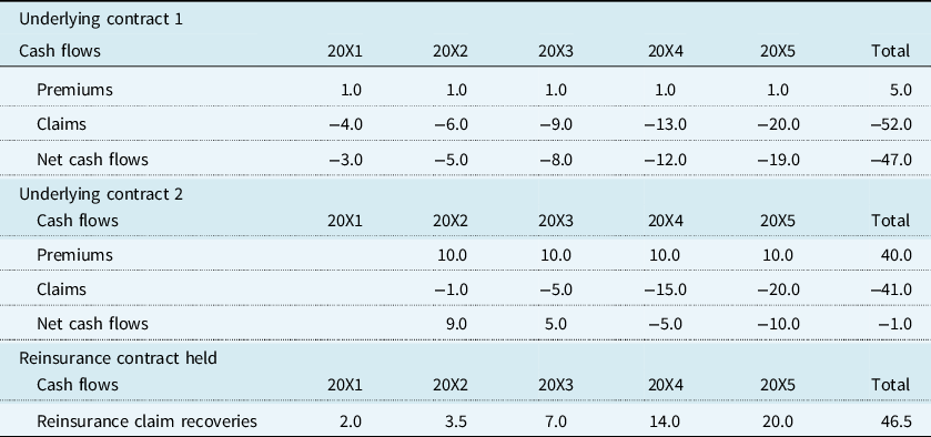
Based on these cash flows, one can generate the following LC run-off patterns as well as an extract of the P&L entries relating to these movements. In addition, one can generate three run-off patterns and P&L entries based on three methods of amortising the loss-recovery component; these three methods (described in detail below) are a result of the various possible interpretations of paragraphs B119F and BC74 (June 2019). The related calculations and illustrations are shown in Tables 32, 33 and Figure 6.
Table 32. Example of Profit and Loss Entries Based on Three Methods of Amortisation for the Loss-Recovery Component
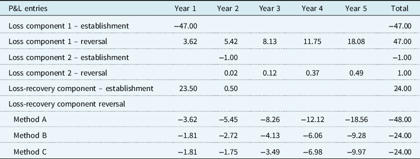
Table 33. Example of Loss-Recovery Component Balances Based on Three Methods of Amortisation


Figure 6. Example of loss-recovery component run-off profile based on three methods of amortisation.
Method A: One interpretation of paragraphs B119F and BC74 (June 2019) could be that the amount by which the loss-recovery component is amortised is itself just a simple sum of the amounts by which the two underlying LC are being (independently) amortised. This route would be practically simpler and relatively easier to follow in the financial statements. However, this seems too simple; in fact, this only works when the underlying contracts are 100% reinsured. In all other scenarios, this method fails to amortise the loss-recovery component to zero by the end of the reinsurance contract. Consequently, this method is not a genuine possibility for companies to use.
Method B: Method B fixes the underlying problem with Method A. To be consistent with how the loss-recovery component was established, it multiplies LC reversal amounts by the percentage of claims that the reinsurance covers. This results in a zero loss-recovery component by the end of the reinsurance contract. Note the operational challenge of this approach whereby the company will have to identify, store and track the percentage of claims it expects to recover from the reinsurance contract for each underlying group of insurance contract it holds to enable this calculation on an ongoing basis.
Method C: Method C arises from one possible reading of BC74 (June 2019), which suggests a different approach entirely. Rather than amortising the loss-recovery component based on amounts by which the underlying LC are amortised (as paragraph B119F could be suggesting as noted above), paragraph BC74 can be read as requiring the systematic reversal of the loss-recovery component to be treated similarly to LC by way of similar methodologies being applied in both instances. In this case, the reversal of the loss-recovery component would be an entirely separate and bottom-up calculation altogether but one that applies the same underlying methodology principles as that used for amortising the loss components. This is operationally and technically more complex but one that could be argued is a technically more superior method. In addition, only minor changes would be required to adapt the loss-component methodology into one that can be applied to loss-recovery components.
All options have competing technical, operational and financial consequences.
Third, whilst the requirements of paragraph B119D appear to be straightforward and prescriptive, there are some important items that have not been addressed in that paragraph. The exclusion of these items has important implications that shall now be considered:
Practical expediency versus technical accuracy
Paragraph BC79 (June 2019) shows that the method prescribed by the IASB for determining the loss-recovery component was swayed in favour of practical expediency rather than technical accuracy. This is important because even though many insurance contracts will have claims as to the primary cash outflow, it does not follow that most will.
Consider a group of onerous underlying contracts that have been identified as onerous in virtue of any other reason than the expected size of the claims (as has been stated by the IASB, in paragraph BC79 (June 2019), to be a reasonable practical assumption to the extent that the loss does not exceed those claims). The group may be onerous because of high acquisition or maintenance expenses or simply because of the RA that is set up.
From one point of view, on technical grounds, it seems inappropriate to make this practical assumption. Whilst unlikely, some entities may now have a tactical incentive to increase market share through unsustainably low premiums or unjustifiably high commissions because shareholders do not need to recognise these losses immediately (at least under the accounting balance sheet). What impacts might this have on the market dynamics? How might competitors respond? How might the regulator respond?
On the other hand, any further exclusions on what cash flows can (or cannot) be included in determining the loss-recovery component would result in an operationally complex and costly approach. From this point of view, the practical assumption is necessary.
(No) risk of reinsurer non-performance
Paragraph B119D does not explicitly require any allowance in respect of the risk of non-performance. However, allowing 100% of future reinsurance recoveries to be recognised as immediate gains is not “best estimate” and is inconsistent with other paragraphs in the Standard that discuss the measurement of reinsurance contracts held. There are hints in paragraphs BC78-BC83 (June 2019) that the non-allowance of the risk of reinsurer’s non-performance in this calculation is a deliberate and necessary consequence of what it means to allow an early recognition of recoveries.
Conclusions
It is clear that there shall be no further amendments in relation to the treatment of reinsurance contracts held. Consequently, companies should determine for themselves how they wish to approach their reinsurance methodology in response to these issues. Whilst going over and above the IFRS 17 requirements is technically and operationally more demanding, and arguably leads to a more accurate reflection of accounts, the costs of doing so may not always exceed the benefits. Companies would consequently do well to pay attention to what the Standard does, and possibly more importantly, does not require.
4.8.5. Sources of mismatches between direct business issued and reinsurance contracts held
There are several potential sources of mismatches when measuring gross business and reinsurance held. This section touches on three such sources: (1) the need to estimate and include future new business when measuring reinsurance contracts held; (2) differences in locked-in discount rates used to measure underlying contracts and reinsurance contracts held; (3) mismatches that arise when VFA business is reinsured.
Estimating future new business
When measuring reinsurance contracts held, IFRS 17 requires companies to estimate the future new business that will be reinsured under those contracts. This requirement only applies to the reinsurance contract held and not for the underlying (gross) unit of account.
Not only does this create technical challenges in relation to how that future new business will be forecast, this may also become a source of future mismatches in the balance sheet and consequently the P&L only if there are differences in how the provision of service is measured between gross and the reinsured business.
Illustrative Example 4.17
This illustrative example is highly simplified. It is important to note that the approach in this example makes two important assumptions:
-
(1) That the company applies a discrete-monthly roll-forward approach when measuring contracts for interim reporting periods.
-
(2) That the company changes the treatment of estimates made at the start/end of prior interim reporting periods.
These are two assumptions that some, but not all, companies will apply in practice.
This is important because the conclusion eventually drawn from this example only follows if this particular approach is adopted in practice (or other similar approaches whereby calculations are performed on, say, a discrete quarterly roll-forward basis).
Companies that only measure contracts on an annual basis (and consequently do not produce interim statements) will not arrive at the same conclusion and may find timing mismatches in the development of results between the underlying contracts and reinsurance contracts held.
Consider a company that enters a 100% quota share treaty on an original terms’ basis. Based on information from its business plan, with necessary adjustments to reflect the expected impacts of any repricing activity and a marketing strategy (or other relevant items), it estimates that 2 direct contracts will be written per month for the next quarter. In reality, it turns out that only 1 contract is written per month.
Each contract has a term of 10 months (but is valued through the GMM) with expected premiums of £60 per month decreasing by £5 each month (total expected premiums = £375) and expected claims of £5 per month increasing by £5 each month (total expected claims = £275). Each contract is, therefore, expected to make the company £100 in total over its lifetime, as shown in Table 34.
Table 34. Example of Future new Business Expected Cash Flows

For simplicity, RA is ignored, and interest rates are assumed to be 0%. It is also assumed that the risk of reinsurer default is zero.
Initial measurement
For the gross unit of account, the company will only recognise contracts as and when it actually writes this business. Consequently, on day 1, it recognises one contract on the balance sheet with PVFCF of −£100 and a CSM of £100 giving a gross LRC of £0.
However, for the reinsurance unit of account, the company will need to recognise estimated cash flows for the 6 contracts it expects under the quota share in this quarter; the PVFCF on the balance sheet will be £600 and the CSM will be −£600 giving a reinsurance LRC of £0 as well.
Therefore, at initial recognition, the requirement to estimate future new business does not create a balance sheet mismatch.
Subsequent measurement
At the end of the first month, the company prepares its monthly results.
For the gross unit of account, the PVFCF for its first contract reduces to −£45 (as £55 of expected gross cash flows have now emerged). Meanwhile, the gross CSM runs off from £100 to £90 based on the coverage units implied by the single contract currently included in the gross unit of account. By this point, the company recognises the second new contract it has written (PVFCF of −£100 and a CSM of £100). This means that by the end of the first month, the gross unit of account now has a PVFCF of −£145, a CSM of £190 and an LRC of £45.
For the reinsurance unit of account, the PVFCF will reduce from £600 to £445. £100 of this reduction is due to the fact that the company expected two contracts to be written in the first month but only ended up writing one. The remainder is based on the £55 of expected reinsurance cash flows that have now emerged.
The reinsurance CSM reduces from −£600 to −£490 (a reduction of £110). £100 of this reduction reflects an adjustment in respect of future service as noted above in the PVFCF: there are now only five expected underlying contracts being reinsured instead of six (and therefore £100 of net cash flows owed to the reinsurer will never transpire). The remainder relates to the CSM being amortised based on coverage units implied by five contracts currently included in the unit of account (instead of the six that was expected to begin with).
Consequently, by the end of the first month, the reinsurance unit of account now has a PVFCF of £445, a CSM of −£490 and an LRC of −£45.
By continuing to track the measurement of the contracts for the remainder of the year until the entire block of business runs off, one can produce Figure 7 and Table 35 that illustrates the PVFCF, CSM and LRC profiles for both the gross and reinsurance units of account.

Figure 7. Example of PVFCF, CSM and LRC profiles for gross and reinsurance units of account.
Table 35. Example of PVFCF, CSM and LRC Calculations for Gross and Reinsurance Units of Account
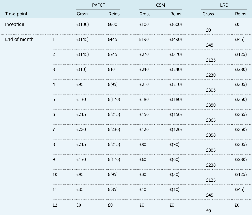
This shows that provided there is a consistent measurement of service being provided between the gross and reinsurance unit of account, then even though there may be differences in the PVFCF and CSM balances initially resulting from differences in estimates of cash flows, these do not necessarily have to result in mismatches resulting in the LRC.
One can reproduce the information above, but this time assume that for the purposes of measuring the reinsurance contract, future new business will only be recognised as and when it is recognised for the gross unit of account. This gives the results, as shown in Figure 8 and Table 36.

Figure 8. Example of PVFCF, CSM and LRC profiles for gross and reinsurance units of account assuming future new business will only be recognised as and when it is recognised for the gross unit of account.
Table 36. Example of PVFCF, CSM and LRC Calculations for Gross and Reinsurance Units of Account Assuming Future New Business will only be Recognised as and when it is Recognised for the Gross Unit of Account

As can be seen, under this approach, the PVFCF, CSM and LRC balances for the gross and reinsurance units of account are mirror images of each other. Further, the LRC balances under this approach are entirely the same as those under the method required by IFRS 17.
The question then is, since estimating or not estimating future new business does not affect the carrying amounts of the LRC for the reinsurance held (for this particular company in this example), and since not estimating future new business could be seen to provide a more intuitive picture of the performance of the business and the effect of the reinsurance, whether the complexity of estimating new business outweighs the expected benefits of this requirement? Apart from the fact that this is a requirement of IFRS 17 and is designed to provide the best estimate measurement of the reinsurance contract held, it is not immediately clear there are many other reasons. Companies in this situation should therefore form their own opinions and discuss with auditors as to the way forward that balances the costs of compliance with requirements against the perceived benefits of doing so.
Discount rate differences
IFRS 17 requires cash flows to be discounted using two separate sets of discount rates when measuring GMM contracts. The PV of future cash flows and RA need to be discounted using the current view of discount rates for the purposes of the balance sheet, but they also need to be discounted using locked-in discount rates for the purposes of calculating the CSM and subsequent adjustments to the CSM.
The locked-in discount rate is based on rates determined at the initial recognition of contracts.
Depending on when gross and reinsurance units of account are recognised, this can consequently result in different interest rates being used to value cash flows for the gross and reinsurance CSMs.
Consider a reinsurance contract entered into in 2018 – this will mean that the reinsurance CSM and all subsequent changes to this CSM will need to be valued at a locked-in curve A. The reinsurance contract covers a group of gross contracts written in 2018, 2019 and 2020, each group valued using locked-in curves A, B and C, respectively.
When there are changes in estimates for future cash flows arising for the 2018 cohort, they will need to adjust both the gross and reinsurance CSM using yield curve A. However, when there are changes in estimates for the 2019 cohort, the gross CSM will be adjusted using curve B but the reinsurance CSM will be adjusted using curve A.
The extent to which the problem arises (and therefore addressed) depends on specific circumstances.
For existing reinsurance treaties that are open to new business being ceded, such as in the example considered here, it is possible that new business termination clauses already exist that result in contract boundaries being set at the end of the notice period point. This was described in detail in section 4.8.2. This means that locked-in rates for both the gross and reinsurance business may end up being similar, if not entirely the same, as and when new units of account are created.
On the other hand, for new reinsurance treaties that are designed to cover closed blocks of in-force business, the discount rate mismatch may be addressed to an extent by adopting a “top-down” discount rate approach (but this would have to apply to all products for consistency rather than just to a subset). Alternatively, more exotic solutions may exist that rely on interest rate swaps.
Reinsuring VFA business
IFRS 17 does not allow reinsurance held to be measured through the VFA. This means that the reinsurance of VFA business needs to be measured through the GMM – a case of a mismatch in measurement models. The justification for this, according to the IASB, is that reinsurance contracts do not provide investment services. Factually, this is incorrect (consider internal reinsurance contracts entered into for participating business before a Part VII transfer or consider funded reinsurance arrangements), but the IASB does not plan to reconsider this further.
This mismatch is problematic because changes in financial risks adjust the CSM under the VFA, whereas they go through the P&L under the GMM.
However, to mitigate this, IFRS 17 offers companies the risk mitigation option of paragraph B115. Exercising this option means that changes in financial risks no longer adjust the CSM under the VFA. Instead, this change goes through the P&L (and consequently aligns the treatment for both the underlying VFA contracts and reinsurance held).
The question to now consider is this: does the risk mitigation option eliminate the potential for any mismatches to arise? Not necessarily.
Consider VFA business that is 100% reinsured. Current interest rates are 2%. At the same time, the company enters into a reinsurance contract, which qualifies for the risk mitigation option (and so is locked into an interest rate of 2% at initial recognition). Assume, for simplicity, the gross CSM is +100 and the reinsurance CSM is −100.
Two changes happen at this point:
-
(1) an interest rate change from 2% to 0.5% – say the impact is 5,
-
(2) an assumption update resulting in a reduction in the expected cost of providing death benefits – say the impact on the locked-in curve is 2 and the impact on the latest curve is 4.
Under the risk mitigation option, the company will recognise + 5 and −5 in the P&L immediately for (1) for each of gross and reinsurance. No accounting mismatch arises.
However, what happens under (2)? This is a change in demographic risk, not a financial risk. The risk mitigation option is silent and instead, the usual IFRS 17 treatment under GMM will apply. Consequently, the company will need to adjust the gross CSM to 104 (based on the latest curve) and the reinsured CSM to −102 (based on the locked-in curve) even though the contract was 100% reinsured. A mismatch arises which then has subsequent impacts on revenue, insurance finance income/expenses and shareholder equity.
Tables 37 and 38 explain this section more generally.
Table 37. Impact of Financial and Non-Financial Assumptions in Gross (VFA) Business

Table 38. Impact of Financial and Non-Financial Assumptions in Reinsurance held (GMM) Business

4.9. With-Profits Funds
4.9.1. Introduction
WP products under IFRS 17 is one of the most discussed subjects by the insurance industry in the UK and overseas. The areas attracting most deliberations are as follows:
-
Aggregation due to the pooled management nature of the products and mutualisation requirements as set out within the standard.
-
Considerations of risk sharing, presence of the Estate, etc.
-
Existence of GAOs on WP policies due to the contract boundary consideration and choice of valuation model as a result.
-
Non-profit business (NP) within WP funds due to the NP being an underlying item for the WP fund and policyholder/shareholder profit arrangement.
-
Variation of types of WP policies and as such a variety of approaches required.
These challenges are discussed in this section in an attempt to demonstrate how they occur, reveal their features and bring them to readers’ attention for further consideration.
4.9.2. Level of aggregation and the Estate
Overview
This section looks at challenges around the level of aggregation for WP business. A broader view of the level of aggregation considerations is covered in section 3.2.
The level of aggregation or grouping is an important aspect of IFRS 17 because it determines at which level the CSM will be calculated and it will ultimately have an impact on how the insurer’s performance will be reported in its financial statements. Companies typically look to achieve the minimum number of groups to both reduce the volatility of the income statement and to minimise the operational complexity.
Paragraph 14 requires that “An entity shall identify portfolios of insurance contracts. A portfolio comprises contracts subject to similar risks and managed together. Contracts within a product line would be expected to have similar risks and hence would be expected to be in the same portfolio if they are managed together. Contracts in different product lines (for example single premium fixed annuities compared with regular term life assurance) would not be expected to have similar risks and hence would be expected to be in different portfolios.”
Further, portfolios are then subdivided into groups no more than 1 year apart according to paragraph 22 (excluding existing business at Transition) and by profitability levels (paragraph 16).
For in-force business at transition, IFRS 17 provides flexibility to group contracts issued more than 12 months apart. This suggests closed funds (or those with very low new business volumes for WP) may have no need for annual cohorts post-transition and a single group may be considered across the whole fund, subject to the fund meeting the definition of portfolio. However, for funds with new business, the split of business into annual cohorts does not reflect inter-generational mutualisation.
Challenges: risk-sharing
Due to the nature of the WP business, additional considerations need to be made when determining the level of aggregation. Risk-sharing is a common feature of WP business, where there are minimum guarantees and the underlying assets are shared across policies. For example, when the return on the underlying assets (e.g. 3%) is insufficient to meet the minimum guarantee of policy A (e.g. 4%), the excess of return above the minimum guarantee of other policies (e.g. policy B – guarantee of 1%) can be used to meet the minimum guarantee of policy A. Policy B could then receive at the insurer’s discretion, either:
-
the minimum guarantee of 1% (the other 1% could be retained by the insurer) or
-
a return of 2% (3% minus additional return paid to policy A).
In the case where this is still insufficient, the insurer will be liable for paying the difference between the minimum guarantee and the return on the underlying assets.
Risk-sharing (also referred to as mutualisation or cross-subsidies) could happen between different generations of policyholders due to the uncertainty of the amounts and the timing of those payments. Is the sharing of risks a strong argument to have the whole fund as a single group?
Paragraphs B67–B69 cover this risk-sharing situation where contracts have “cash flows that affect or are affected by cash flows to policyholders of other contracts”. Due to the level of aggregation requirements, paragraph B68 covers contracts, which affect the cash flows of contracts in another group and requires an adjustment to the fulfilment cash flows to avoid double counting.
This requirement in paragraph B68 means that a company will have to estimate and adjust each group’s fulfilment cash flows, and the more groups there are the more estimations at a potentially very granular level will need to be made, which leads to a higher operational complexity. An example is provided in paragraph B69: “to the extent that payments to policyholders in one group are reduced from a share in the returns on underlying items of CU350 to CU250 because of payments of a guaranteed amount to policyholders in another group, the fulfilment cash flows of the first group would include the payments of CU100 (i.e. would be CU350) and the fulfilment cash flows of the second group would exclude CU100 of the guaranteed amount.”
An advantage of having less groups is that some of them will potentially not need to have their fulfilment cash flows adjusted, allowing the CSM to be calculated at a more aggregated level, reducing the operational complexity and more accurately allowing for the risk-sharing.
However, there is no practical approach described in the Standard for the estimation of the fulfilment cash flows adjustment due to risk-sharing. Consequently, paragraph B70 explicitly mentions different practical approaches may be adopted, including the estimation at a higher level than the level of aggregation required.
There have been several discussions around the annual cohort requirement and whether it should be removed or amended. Concerns raised to the IASB by stakeholders include the annual cohort requirement not reflecting the intergenerational sharing of risks, arbitrary CSM allocations due to adjustments to fulfilment cash flows and higher implementation costs. However, the IASB has carefully considered them and concluded that risk-sharing is not by itself sufficient to make annual cohorts unnecessary.
As summarised in the article “IFRS 17 Insurance Contracts – Why annual cohorts?”,Footnote 18 the main reasons given by the IASB include:
-
The insurer usually shares the risk with the policyholders and this leads to significant differences in the financial performance of the annual cohorts, especially for those with minimum guarantees. In addition, contracts, where all types of risks are shared fully across policyholders, are very uncommon.
-
The IASB believes that the adjustments to fulfilment cash flows have a clear purpose and that tracking contracts with mutualisation by annual cohorts provides useful information to users of financial statements around how the business is expected to develop.
-
The significant benefit to users of financial statements outweighs the additional complexity to accounting systems the annual cohort requirement introduces.
Consequently, the IASB believes that any change to this requirement introduces a great risk of an “unacceptable loss of information” to users of financial statements and will not preserve the faithful representation of an insurer’s financial performance.
Challenges: the Estate
Following paragraph 14, the consideration of the different risks between product groups is a sensible starting point for the level of aggregation. However, when considering WP, the extent to which the impact of risks on the entity varies by products will depend on the entity exposure, e.g. extent that the Estate absorbs risks and hence losses. For many WP funds, much of the risk is absorbed by the Estate and, from the entity perspective, the vast majority of risk (to shareholders) is simply market risk across products. Further, given risk sharing exists through the Estate all products are managed together in one fund, which might suggest they can be managed as one portfolio.
Paragraph B71 allows for the Estate by allowing a liability to be recognised for the fulfilment cash flows arising from all groups when all the coverage has been provided to contracts within a group. This suggests that when all contracts in a group are extinguished, cash flows recognised via the adjustment required in paragraph B68 would automatically fall within a liability recognised according to paragraph B71 (if the option provided in B71 is used). However, if the closed fund is allowed to be considered as one single group, the contribution to the Estate will not happen until coverage has been provided to the last policy of the fund.
Presumably, transfers between paragraphs B71 and B68 can be made to and from the underlying item to avoid any complications that could arise as the fund runs off, albeit depending on the exact solution, it can give rise to quite volatile movements between equity and CSM.
Conclusion
As with other business lines, in determining the level of aggregation for WP business, companies typically look to achieve the minimum number of groups to both minimise the operational complexity and reduce Income Statement volatility. More granular level of groups could result in more onerous contracts being recognised, as some or all of the offsetting benefits of profitable contracts may be separated into other groups. Intergenerational risk-sharing and the management of the WP fund appear to be strong arguments to support the WP funds to be considered as one single group, although these arguments are more applicable to reporting to policyholders and the management of mutuals, rather than to external financial stakeholders. Companies will need to comply with the annual cohort requirement and individually assess the specifics of their WP funds against the IFRS 17 requirements.
The Standard allows for the risk-sharing to be considered via an adjustment to the fulfilment cash flows and it allows for the Estate through a liability for fulfilment cash flows arising from all groups. However, no prescription is made as many different practical approaches could be adopted and considering the Estate and the shareholders from an entity perspective could have an impact on the approach chosen. Therefore, it is up to the companies to decide how to deal with the measurement of the Estate and the adjustments to the fulfilment cash flows.
The allowance for the Estate in run-off needs careful consideration in order to be aligned with the economics of the business.
4.9.3. Guaranteed annuity options
Many WP contracts feature guaranteed annuities, often in the form of a guaranteed minimum rate of conversion to an annuity at retirement, referred to as GAOs. Once the option vests, the annuity itself partakes no further in the pooled profits in the WP fund – i.e. it is a standard non-profit annuity. As such, from a practical perspective, companies generally view the option vesting point as a cessation of the original WP contract and the writing of a new annuity contract. IFRS 4 and Solvency II treatment generally reflect this view.
The approach to managing the resulting annuities varies between companies, with three possible approaches:
-
The annuity is written in the WP fund and the WP policyholders bear the associated longevity risk.
-
An internal buy out into the entity’s non-profit annuity fund takes place. A market price for taking on the liabilities is agreed between the WP fund and the entity. This “premium” will likely include an allowance for risk and a profit margin for the entity and is paid by the WP fund to the non-profit fund. The value of this “re-price” exercise, therefore impacts the existing WP policyholders. The WP fund ceases to bear any liability or risks, as these are passed to the non-profit fund which now bears the longevity risk, etc.
-
An external buy out to the open market takes place. Neither the WP fund nor the entity has any remaining liability to the annuitants and all risks associated with the contract are passed to the external party.
The current industry view is that the IFRS 17 requirements make it challenging to continue the current approach of considering the two phases of these contracts separately. This results in a number of significant issues:
-
Measurement model: Looked at on a standalone basis, the savings or accumulation phase of the GAO contract is likely to qualify the contract for the VFA, whereas the annuity phase on its own would be measured under the GMM. However, once the measurement model is assessed for a contract there is no ability to change this, even if the nature of the contract changes over time, as with the GAO contracts. The first question is, therefore, which model should be applied for the whole contract. To assess this the VFA requirements in paragraph B101 apply. There are two key points to consider, (a) what is the variability of the value of the pay out to customers if the guarantees are in the money and (b) how “substantial” should be interpreted when the pay out to customers in only based on the underlying for a proportion of the term of the contract. Considering these in turn:
-
○ Many GAOs are heavily in the money. The variability of the policyholder payout will depend on the details of the guarantee, which will vary by fund. For example, for many UK GAOs, it is the annuity factor that is guaranteed (rather than the total annuity amount) so, even if in the money, the policyholder share will vary with the returns earned on the underlying funds.
-
○ The conditions in paragraph B101 do not deal with the situation where the policyholder only participates in a share of the underlying items for a proportion of the policy term. The VFA requirements refer to the entity paying a “substantial share” of the return on the underlying to the policyholder (paragraph B101(b)) and the entity expecting a “substantial proportion” of any change in the amounts to be paid to policyholders to vary with the change in the underlying items (paragraph B101(c)). It is open to debate whether substantial should be interpreted to suggest that, if the policy payout is only linked to underlying items for a short duration, then the contract meets these conditions and qualifies for VFA. If so, where should the cut-off be in terms of, say, the number of years till the contract vests? Industry interpretation on this point is still developing.
Assuming, the conclusion is that the VFA model applies for the whole contract, this gives rise to some interesting conceptual challenges as to how to apply the VFA model to an annuity. For example, it is hard to see that there are any underlying items in a non-profit annuity. Beyond these technical concerns, accounting mismatches are likely to arise given under the VFA model economic variance adjusts the CSM, whereas the economic variance from the assets held to match the annuity cash flows will go through the P&L.
If the conclusion is that the GMM applies for the whole contract, then the challenges and accounting mismatch arises during the savings phase.
-
-
Identifying annuity contracts that were originally WP contracts with GAOs:
For many firms, once a contract moves into its annuity phase, a new policy is set up on the admin system, with no link back to the original WP contract. Hence it may be very challenging, if not impossible, to distinguish GAO contracts from the general annuity population. With the true inception date and history of a contract unknown, an entity could be forced into applying a fair value approach for a large proportion of its annuity book. This could have significant implications on the size of the CSM at transition.
-
A very long coverage period:
With the savings and retirement phase within the same contract, an entity will have a very long coverage period, with very different types of service provided in both phases. An entity will need to think very carefully about how coverage units (covered in section 4.6) can be appropriately determined across each phase.
-
Determining the RA:
For contracts currently in the savings phase, entities will need to consider the future risks on the annuity in calculating the current RA.
-
Distinguishing financial and non-financial impacts on future cash flows:
Modelling the annuity period within the contract boundary requires consideration of the different assumptions that will impact the expected future annuity cash flows – this will include financial (fund growth rates) and non-financial assumptions (e.g. take up of the option and longevity), some of which may be quite entwined and therefore hard to distinguish between. If the VFA model applies, then the impact of all assumption changes will go to CSM. However, if GMM applies, then there may be a requirement to separate financial and non-financial assumption impacts (section 4.9.5 considers some possibilities in this respect).
So, given these issues, is there anything in the Standard that would allow separating the two phases of the contract? A number of possibilities have been considered by the industry:
-
Is the WP element a distinct investment component?
Paragraph B31(a) states that for an investment component to be distinct, it and the insurance component must not be highly interrelated. Given the clear interdependence between the cash flows in the WP contract and on the guaranteed annuity, it is concluded that there is no distinct investment component.
-
Is there a contract modification at the point of vesting?
Paragraph 72 requires that for a modification to occur, the terms of the contract must have been modified. This is not the case here as the guarantee existed from inception of the contract. The practical fact that a policy is set up as a new policy on the admin system does not in itself qualify as a contract modification. This paragraph also clarifies that the exercising of an option is not a modification.
-
Is there a contract boundary at the point of vesting?
If the annuity is bought out at this point then there may be an argument for a contract boundary. If the buy out is external then clearly there is a contract boundary and a new contract in a new entity. However, could there potentially be a contract boundary if the annuity is bought out internally? This is considered below.
As above, let’s consider whether there is a contract boundary at the point where the vested annuities are bought out by the non-profit fund of the same entity which owns the WP fund (i.e. an internal buy out). Paragraph 34 sets out the requirements for determining when a substantive obligation ends, consequently creating a contract boundary. It requires either that:
-
(a) The entity has the practical ability to reassess the risks of the particular policyholder and, as a result, set a “price” that fully reflects those risks
or
-
(b) the entity has the practical ability to reassess the risks of the portfolio of insurance contracts and, as a result, set a “price” that fully reflects the risks of the portfolio. (For the substantive obligation to end, then in addition to this criteria being met, the pricing of the premiums for coverage up to the potential contract boundary must also not take into account the risks that relate to periods after the reassessment date).
For a GAO contact being internally bought out from the WP fund, the risks of a particular policyholder are reassessed and a price is set that fully reflects those risks. However, the premium is charged by the entity to the WP fund, and hence effectively to the remaining policyholders, not the policyholder of the contract in question. There are differing views on whether this meets the requirements in paragraph 34, although the argument for a contract boundary in this way seems to be losing strength in the industry.
Contracts with similar issues to the UK GAOs exist across Europe and in Canada, and there has been significant lobbying to the IASB to highlight industry concerns for the treatment of such contracts whose nature changes over time. However, in February 2020, the IASB decided not to make any changes to the Standard to address these concerns and not to issue any guidance on applying the Standard for such contracts. However, in coming to this conclusion, the IASB pointed to the newly extended scope of the risk mitigation option as a potential option to mitigate the accounting mismatch created by measuring the annuity phase under the VFA. The industry is still to explore the possibility. However, whilst this may help the commercial implications of this issue, the operational and technical challenges will remain – in fact, applying the risk mitigation option to this business will add additional complexity. Also, significantly, the risk mitigation option can’t be applied retrospectively at transition, and of course does not help identify ex-GAO contracts.
In conclusion, this is an area where the industry continues to be highly concerned, both in terms of the operational complexities of applying the Standard’s implied interpretation and the commercial implications this has for the bottom-line numbers and usability of accounts.
4.9.4. Non-Profit business written within a with-profits fund
It is not uncommon to have NP written within a WP fund, especially in the UK and continental Europe market. Economically, the profits earned on these contracts are distributed wholly or partially to WP policyholders depending on the setup of the fund, i.e. they are effectively underlying items of the WP fund. In the case where profit is only partially allocated to WP policyholders, the remaining profit will be allocated to the entity, e.g. through the 90/10 gate.
However, NP policies are likely to need to be grouped separately based on the level of aggregation requirements on exposure to similar risks and managed together. As a result, measurement of the group in isolation would lead to a CSM (assuming profitable) or LC (assuming it is onerous).
An IASB paperFootnote 19 on mutuals states that (emphasis added):
“Mutual entities may issue conventional insurance contracts that do not provide policyholders with a residual interest in the mutual entity, for example non-participating insurance contracts…The requirements of IFRS 17 apply to these contracts regardless of the fact that they: have been issued by a mutual entity; and are underlying items for other contracts. Consequently, groups of such contracts are expected to have a CSM”
In order to calculate CSM of NP within a WP fund, here is a list of considerations that a company should think through.
-
Definition of CSM:
It may be debatable whether the CSM of NP is the same as the normal CSM. The IASB paper is clear that a CSM on the NP within a WP fund should be calculated, but it is less clear whether this CSM is from the entity’s perspective or from WP shareholders’ perspective because the profit from this NP may be shared between them. For example, if 100% of the profit is allocated to WP policyholders, this NP business should have no CSM from the company’s perspective because the shareholders do not share any profit from the NP business. This should be further explored across the industry to ensure a consistent disclosure on how the CSM of NP should be accounted.
-
Measurement Model:
It is likely that the NP business written in a WP fund will follow the GMM model, e.g. protection business or similar. In this case, the company needs to define clearly what constitutes the underlying items of the fair value valuation for the WP fund when this NP business flows through. If the company defines the profit from NP as a single item, the VFA calculation for the WP fund will be easier. Whereas, if more than one item needs to flow through the VFA calculation, the process can become messy very quickly. Also, in the case where NP business is onerous, the company should define clearly how the LC should be recognised and, more importantly, allocated to different cohorts of WP policyholders. This is easier when asset share is calculated because the company should have more information to support this allocation. But, it will be much more difficult when asset share is not always calculated.
-
Risk adjustment:
The non-financial risk sharing between NP and the WP fund may blur the line between how the RA should be calculated. For example, whether RA of NP should be based on the diversification at the WP fund level or at the NP level.
This becomes more complicated if the non-financial risk is shared all the way up to the shareholder level when the profit of NP is partially allocated to WP policyholders and shareholders. In this case, the diversification benefit could be at the shareholder legal entity level.
Fundamentally, the approach taken should be consistent with the Principle and Practice of Fund Management (PPFM), or a similar document that sets out how the fund is managed in other jurisdictions.
-
Reinsurance:
If WP enters a reinsurance to cover the risk arising from both NP business and other parts of WP fund, e.g. mortality cover to cover all business, there will be a question on how this reinsurance can be split into NP business and the WP fund. This becomes especially tricky if the coverage is not a proportionate reinsurance where the linkage between reinsurance and individual level of aggregation of underlying contract is not clearly mapped.
-
Analysis of change:
In the case where NP business is under GMM, the financial assumption changes in relation to NP business will flow through the CSM of WP business as an intermediate step before feeding into the P&L in the entity’s financial statement.
4.9.5. Additional challenges for non-UK-style with-profits funds
Overview
IFRS 17 prescribes two main approaches for CSM computation, i.e. GMM and VFA. The second approach is only applicable to direct participating products, which meets the requirements of paragraph B101. Whilst many participating products are expected to meet these requirements, this will not be the case for all. Such indirect participating products will be measured under GMM by default as described in section 4.5.3 strictly following the locked-in requirements. Alternatively, an entity may choose to apply permitted modifications to the GMM with respect to discretionary participating features described in this section.
Indirect participating products
As a quick recap on the indirect participating product, these contracts have benefits which are not fixed in nature, but they fail to meet the criteria mentioned in paragraph B10.
Some examples of contracts that may not meet the above conditions include:
-
Anon-participating savings contract where additional returns are declared by the entity based on some index or fund performance but there may not be any direct linkage of the return with the underlying asset, it being more based on the discretion of the entity.
-
A WP contract with high guarantees, due to which the benefits may not vary substantially with the change in fair value of underlying asset.
Modified approach
Paragraphs B98-B100 deals with the treatment of discretionary feature of these indirect participating contracts within the GMM.
Under GMM, the entity uses locked-in assumptions for economic assumptions, comprising discount rates and any adjustment for financial risk. Typically, any discretionary crediting rate will classify as an economic assumption. The standard, however, exempts the entity, allowing it to unlock the discretionary rate at subsequent measurement. For example, in the case of WP product that failed to meet the criteria of paragraph B101, the initial projection may include bonus rates as say 5% each year. After poor experience, the entity may reduce the current year bonus rate to say 4% and further down to say 3% in future.
To the extent this affects fulfilment cash flows, i.e. change in fulfilment cash flows resulting from a change in discretionary rate, this will adjust the CSM. Any implications of the change in rate on current period cash flows will continue to flow in the P&L.
One important aspect of this modification is that the entity should be able to clearly distinguish at the start of the contract the discretionary element within the cash flows, separate from discount rates or any financial risk assumption used. These economic assumptions will continue to be on a locked-in basis whilst measuring the effect of change in FCF due to the change in discretionary rate.
However, it is also important to note that when measuring fulfilment cash flows to be held on the balance sheet at the valuation date, the discount rates will continue to be the current assumption, and consistent with any changes in the discretionary rates. Only for the purpose of calculating the adjustment to the CSM do the discount rates remain locked in.
Operationally, this would mean an additional step in the computation of CSM to identify a change in discretionary rate separate from any other assumption change but this should be relatively straightforward if the discretionary element can be clearly identified.
4.9.6. Further reading
Readers may find the following documents useful to consult:
-
Institute of Chartered Accountants of England and Wales (ICAEW): Non-Profit Business in a With-Profits Fund
-
Institute of Chartered Accountants of England and Wales (ICAEW): Accounting for annuities that have vested from with-profits contracts under IFRS 17
-
EFRAG TEG Paper 06-03 – 6 May 2020: Contracts that change their nature over time – Issues paper
-
IFoA IFRS 17 Transversal Working Party: Impact on UK with-profits business
https://www.actuaries.org.uk/documents/ifrs-17-impact-uk-profits-business-20200128.
-
Singapore Actuarial Society: IFRS 17 Workgroup Resources: Par Fund and VFA Measurement
5. Transition
5.1. Introduction to Transition
This section considers the transition requirements that apply when an entity presents financial statements applying IFRS 17 for the first time. This section sets out:
-
An overview of the transition requirements under IFRS 17.
-
An overview of the three transition approaches as set out in Appendix B of the IFRS 17 standard, which the Working Party will refer to as:
-
○ “Full retrospective approach” – FRA.
-
○ “Modified retrospective approach” – MRA.
-
○ “Fair value approach” – FVA.
-
-
Discussion around the potential implementation challenges and consideration in selecting an alternative approach where the FRA is impracticable, which includes comparing the MRA against the FVA as well as potential ways firms could approach their transition strategy.
5.2. What are the Transition Requirements?
IFRS 17 applies to entities for annual reporting periods on or after 1 January 2023, the “date of initial application”, (though earlier application is permitted). However, entities are required to provide IFRS 17 comparative financial statements as of the beginning of the period immediately preceding the date of initial application. For companies with a 31 December year end, this gives a transition date of 1 January 2022.
To provide these comparative statements, entities will need to calculate the following for each group of contracts, as at the transition date, using one of the three transition approaches as set out in Appendix B of the IFRS 17 Standard:
-
the carrying value of the liability (or asset), with separate measurement of the RA and the CSM or LC,
-
the “locked-in discount rate”, being the discount rate used for CSM accretion,
-
the accumulated OCI (if the OCI disaggregation option is elected),
-
the balance of unamortised insurance acquisition cash flows (unless the fair value approach is used).
5.3. Overview of the Transition Approaches
5.3.1. Full retrospective approach – FRA
IFRS 17 requires that entities apply the Standard retrospectively (i.e. apply the measurement requirements to groups of insurance contracts as if IFRS 17 had always applied) unless it is “impracticable” for the entity to do so (as defined by IAS 8 “Accounting Policies, Changes in Accounting Estimates and Changes in Accounting Policies”). This is referred to as the “fully retrospective approach”.
Paragraph BC378 (May 2017) highlights that the IASB recognised that the measurement of several types of items needed for the FRA would often be impracticable. Consequently, the modified retrospective approach and the fair value approach were developed in response.
However, whilst there exist specified modifications under the MRA the IASB has made clear that this does not preclude the normal use of estimatesFootnote 20 as part of the transition. In the staff analysis of requests from stakeholders to permit entities to develop their own modificationsFootnote 21 the staff say,
“When an entity applies a requirement retrospectively, it may be necessary to make estimates. When the entity cannot estimate an amount retrospectively, the specified modifications allow the entity to instead estimate a proxy for the retrospective determination of that amount.”
Therefore, firms are permitted to use estimates when using the FRA (and the MRA) and the use of estimates does not preclude a company from using the FRA. These estimates would need to be discussed and agreed with auditors and a company should be aware that if an estimate is in breach of the requirements of the FRA (i.e. the use of hindsight), then it would obviously not be permitted.
An important aspect of the IFRS 17 requirements for transition is that the Standard does not establish a “pecking order” between the MRA and the FVA. If the FRA is impracticable to apply, entities have a free choice in applying either the MRA (where they are able to) or the FVA for the transition. The policy choice of applying MRA or FVA will potentially lead to different levels of opening CSM balance, and consequently their future earnings and balance sheet position. Companies should investigate the practicability, relative costs and benefits of the two approaches. Further details on the definition of impracticability and the cost versus benefits of the respective approaches are discussed in section 5.4.
Figure 9 shows the hierarchy of the application of transition requirements to a group of insurance contracts.
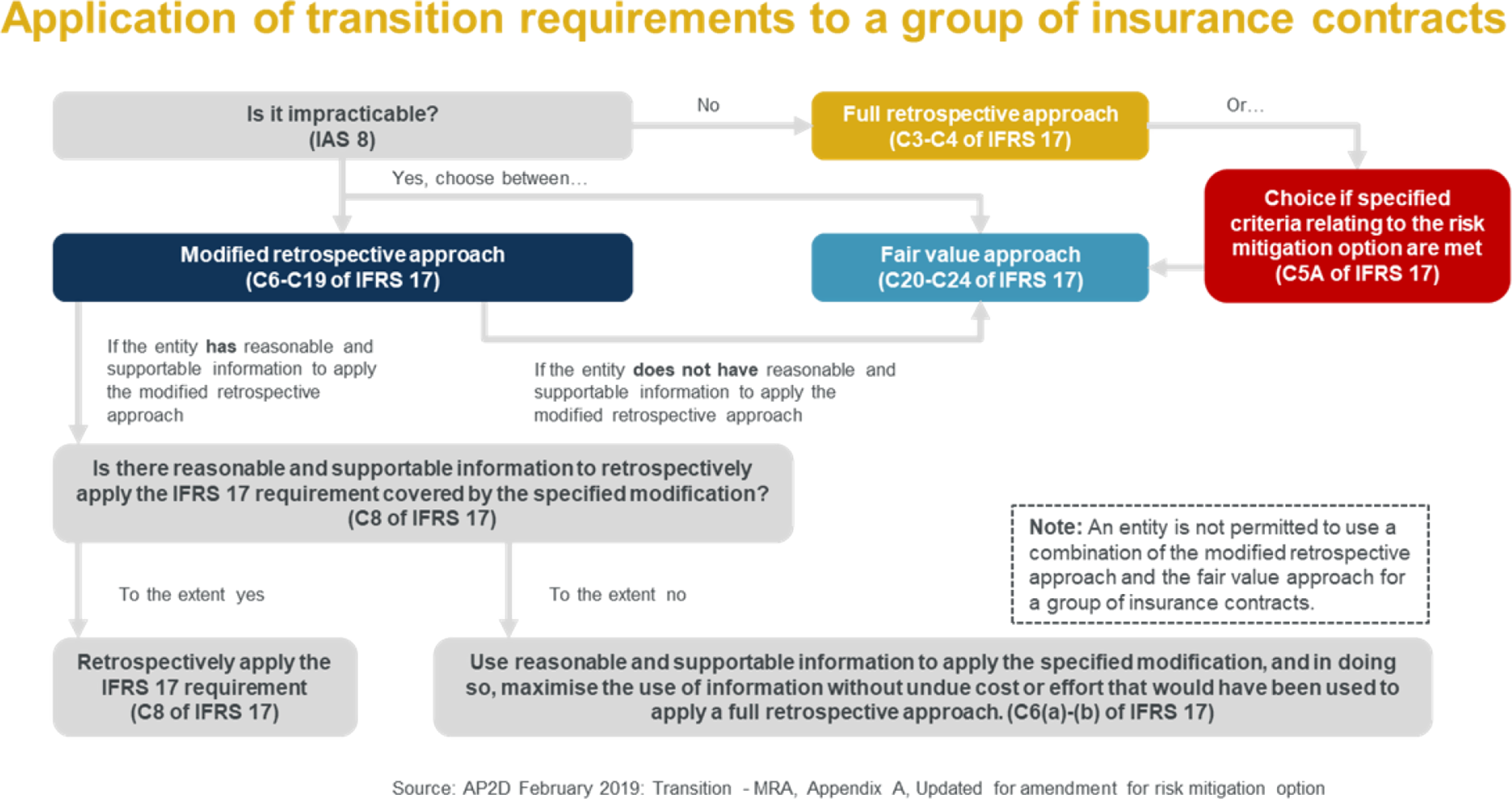
Figure 9. Application of transition requirements to a group of insurance contracts.
5.3.2. Modified retrospective approach – MRA
The MRA offers a number of specific permitted modifications to the FRA in various areas of the Standard, generally to address areas where hindsight might otherwise be required. For GMM business there is a range of permitted modifications – to be used only where these are required – whereas for business under the VFA, a more prescribed modified approach is set out.
The intention of the MRA is to offer a method that maintains comparability of results, whilst recognising that companies will often lack data for a full retrospective calculation. This section gives an overview of the MRA and the permitted modifications under this approach. Details of some of the advantages and disadvantages of the approach can be found in section 5.4.2.
If the MRA is impracticable, companies must use the fair value approach by default.
Permitted modifications – GMM and VFA
The MRA intends to achieve the closest outcome to the retrospective application as possible using reasonable and supportable information available without undue cost or effort. This is achieved through specific modifications to a full retrospective calculation, as set out in the Standard.
For contracts following the GMM, specific modifications are available in a number of areas, including the estimates of future cash flows, the calculation of the RA, the setting of the discount rate, the amortisation of the CSM. The MRA also allows for the grouping of annual cohorts, where there is insufficient data to perform a retrospective calculation at this level. Table 39 summarises the permitted modifications under the GMM approach.
Table 39. Permitted Modifications under the GMM Approach

These modifications provide relief from the requirements of the FRA where necessary, and act as a proxy for that approach. They generally reduce the need for historic estimates (that may involve hindsight), replacing these with estimates as per the transition date, and actual historic data.
There is a requirement to use as few modifications as necessary, which means companies will need to demonstrate for each modification used that the corresponding FRA is impracticable. Firms must also use reasonable and supportable information to apply each specified modification and maximise the use of information without undue cost or effort that would have been used to apply a full retrospective approach.
For contracts measured under the VFA, the method under the MRA is more prescribed (see paragraph C17), but again makes use of historic actual data to estimate the CSM or LC at inception, before rolling this forward to the transition date. Following the permitted MRA, the CSM or LC at inception is estimated as:
-
(a) the total fair value of the underlying items at the transition date;
-
(b) minus the fulfilment cash flows at the transition date;
-
(c) plus or minus the following adjustments;
-
i. add back the amount charged to policyholders (including amounts deducted from underlying items) before the transition,
-
ii. deduct the cash outflows that occurred before the transition and that did not vary based on underlying items (e.g. fixed expenses),
-
iii. deduct the change in RA caused by RA release before the transition and estimate this amount by reference to release of risk for similar insurance contracts issued on transition,
-
iv. deduct insurance acquisition cash flows paid before the transition date that is allocated to the group (those not allocated to the group are recognised as an asset for insurance acquisition cash flows applying paragraph 28B).
-
If this computation results in a CSM at inception, then the CSM at transition is calculated by deducting the amount of CSM that relates to services provided before the transition. The entity shall estimate the amount of CSM that would have been recognised in P&L before transition by comparing remaining coverage units at transition with the ones before the transition. Otherwise, if this computation results in a LC at inception, an entity adjusts the LC to nil and increases the liability for remaining coverage excluding the LC by the same amount.
There are also a number of permitted modifications relating to the determination of insurance finance income or expenses and the calculation of other comprehensive income (OCI) where an entity might struggle to calculate these retrospectively.
Conclusion
In offering a modified approach to retrospective application of the standard, the IASB recognised that it would often be impracticable to carry out a full retrospective calculation. There are clearly areas that may offer some relief to companies, and some may find that the financial result of adopting the MRA is preferable to the use of the FVA.
However, the MRA does not give companies free reign to approximate the CSM at transition with the best information they have available, though the use of estimates will be necessary for any retrospective calculation (full or modified), and discussion of this with auditors will be important. Given these limitations, the MRA will be an approach that may be acceptable for some, but not others.
5.3.3. Fair value approach – FVA
As outlined above, if a full retrospective calculation is impracticable, then the standard permits entities to choose between the MRA and the FVA. If the MRA is impracticable, entities must apply the FVA.
This section provides an overview of the basic calculations under the FVA. Further details on some of the possible approach firms could use in determining the FV and the potential challenges they may face in doing so are provided in section 5.4.3.
The calculation required to determine the FV CSM or loss component
Under the FVA, the CSM or LC at the transition date is calculated as the difference between the FV of the liabilities for a group of contracts, applying IFRS 13, and the fulfilment cash flows for that group, applying IFRS 17, at that date.
If the FV of the liabilities is greater than the fulfilment cash flows, the difference is recognised as a CSM on the balance sheet. On the other hand, if the FV of the liabilities is less than the fulfilment cash flows, the difference is recorded as a LC of the liability for remaining coverage.
Once the opening CSM or LC balance at the transition date has been determined, all subsequent calculations for these balances must revert to the usual requirements of IFRS 17.
Note that whilst it is possible, it will not be commonly expected for LC to arise when using the FVA as most calculations required to arrive at the FV liabilities will result in a higher FV liability than the fulfilment cash flows (e.g. the inclusion of the cost of holding capital that a market participant would require for accepting these obligations).
5.4. Potential Implementation Challenges and Considerations
5.4.1. Definition and application of impracticability
IAS 8: Accounting Policies, Changes in Accounting Estimates and Errors defines applying a requirement as impracticable when the entity cannot apply it after making every reasonable effort to do so. This requires at least one of the following to apply:
-
(a) The effects are not determinable.
-
(b) It requires assumptions about what management’s intent would have been.
-
(c) It requires significant estimates and it is impossible to distinguish what information would have been available at the time, based only on circumstances at the time.
IAS 8 clarifies that when considering (b) and (c), hindsight must not be used. This is a challenge for many companies in determining whether a given scenario meets the above criteria.
Before IFRS 17, the IASB had previously noted that “an assessment of undue cost or effort was too subjective to be applied consistently by different entities…Impracticability Is the only basis on which IFRSs allow specific exemptions from applying particular requirements when the effect of applying them is material” (BC36, IAS 1).
Therefore, although it appears clear that companies should not assess whether there is undue cost or effort involved, whether the effects of retrospective application are determinable in practice or whether they involve hindsight may be a matter of debate or judgement. In many cases, there may be incomplete historic information available, or information that suggests how an accounting policy may have been implemented historically if it had existed, without proving this.
Ultimately, this is a topic that individual firms will need to come to a view on, and resolve with their auditor. This will need to be demonstrated first to prove that a full retrospective approach is impracticable, and second for each modification required under the MRA.
The following sections explore some of the things that firms may wish to consider when deciding on whether to adopt the MRA or FVA where implementing the full retrospective is impracticable.
5.4.2. MRA – potential advantages and disadvantages
Given the free choice available where a full retrospective calculation is impracticable, companies can assess the advantages and disadvantages of MRA and FVA, both from an operational perspective as well as the impact on their financial results.
For contracts under the VFA, such as UK-style WP business, the proxy method under MRA could be significantly less onerous than a full retrospective calculation. The fact that retrospective calculations of liabilities for WP business have been required for a number of years under the UK regulatory regime means that the availability of historic actual cash flow data may be less of an issue here than for some other products. This is also an area where the nature of the business means that defining FV can be particularly challenging – again making an MRA potentially more appealing.
Some companies may find that the issues they face with a full retrospective calculation are limited to specific areas – such as the calculation of the RA or discount rate. If a historic calculation of the RA is found to require hindsight, then the modification available under the MRA provides a route for a calculation that is largely in line with an FRA, whilst avoiding this issue.
However, a view expressed by many in the industry (as recognised in IASB discussions) is that the MRA is too restrictive, making it costly and burdensome to apply.
The approach is deliberately limited to specific modifications. This may be seen as overly restrictive in cases where data is available to support an estimate of the CSM that companies deem to be more in line with the FRA than the calculation under the FVA, but the method doesn’t meet the specific requirements of the MRA.
A specific restriction noted in the MRA concerns the treatment of financial assumptions. The MRA allows for historic estimates of future cash flows to be based on estimates at the transition date, adjusted for actual historic cash flows. However, a result of this is that it reflects the financial assumptions as at the transition date, with no allowance to adjust these to the assumptions that would have been used at initial recognition, where these are known. This may particularly be an issue for companies writing long-term index-linked business (such as annuities), where inflation assumptions may vary significantly between initial recognition and transition.
Some companies may find that a full retrospective calculation is impracticable, due to a lack of available historic data on projected cashflows, at the required level of granularity. Although there is some relief available from the permitted modification to group annual cohorts of business, this is an issue that will remain for some.
5.4.3. FVA – different approaches to the calculation
The FV of a liability needs to be calculated from the perspective of a market participant operating in the same principal (or most advantageous) market. It is the hypothetical exit price at which the liability will be transferred in an orderly transaction between market participants at the measurement date.
Once the FV of the liability has been arrived at, for which a number of possible methods are described in this section, companies can follow the steps in section 5.3.3 to derive the resultant CSM or LC.
Use observable market prices
One theoretically possible method is to set the FV of the liabilities in accordance with observable market prices for such contracts. Companies will need to consider whether the data is representative of the business being valued (e.g. type of business, date of valuation, etc.) and the adjustments that might be needed. For this reason, the conclusion is that it is unlikely for there to be readily usable prices to identify the FV of a liability simply by looking towards the market and work will be required to consider the information available before it is used.
Adjust the fulfilment cash flows
Companies could make several adjustments to their fulfilment cash flows to arrive at the FV of liabilities. Allowances could be made, e.g. for the risk of the company’s own non-performance for groups of contracts (note this is mandatory under IFRS 13) or different underlying demographic or attributable expense basis (e.g. because a market-participant may have different economies of scale or because it has different underwriting, claims management and policy retention practices). Adjustments may also include an allowance for the return a market participant may require for accepting the liability and the risks that come with it.
Use a cost of capital or IRR approach
Under this method, companies could estimate the cost of capital or IRR a market participant will require to take on the obligations for the group of contracts being valued. One possibility could be to calibrate the company’s own solvency or economic capital requirements to that of an average market participant’s capital requirement and then apply a weighted average cost of capital needed by the shareholder of that participant.
Leverage existing EV or SII calculations
Existing EV or SII calculations could be used as one way of approaching the methods of adjusted fulfilment cash flows and using a cost of capital approach instead of approaching the calculations from a blank slate.
5.4.4. FVA – difficulties in determination (calibration, judgement, etc.)
The main challenge with the FVA is in judgement and calibration. As highlighted in the preceding section, there are different methods that firms could adopt in calculating the FV CSM (e.g. adjusting the fulfilment cash flows, using some form of cost of capital or IRR approach or even using existing embedded value or Solvency II metrics). Ultimately the challenge is that any method chosen will involve the application of judgement and companies will need to be able to justify these.
Areas, where judgements and calibrations might be required, include determining the level of the RA used, the profit loading included or the discount rate or the IRR assumed. This requires companies to find sufficient credible data (either externally or internally) and qualitative arguments to support the FV of liabilities that they calculate.
Consider various illustrative scenarios and possible challenges that highlight the complexities of the fair value approach:
-
A German insurer manages a closed book of business that has been reinsured externally to a US reinsurer; assume a quota share with 80% of risk ceded. The book is to be transitioned using the fair value approach. Notwithstanding the need for gross and reinsurance business to be valued separately, given the low retention of the business, should the market participant demographic and economic assumptions for the gross business be based on a market participant in Germany or the US?
-
A UK insurer applies the Standard Formula under SII for determining capital requirements. The UK market is a mix of participants of various sizes applying the Standard Formula or partial internal models or full internal models. There are often separate views of capital companies hold based on their own economic capital models. How sophisticated does this UK insurer’s approach need to be in assessing what a market participant’s view of cost of capital will be?
5.4.5. FVA versus MRA
Should a company apply the MRA or the FVA?
Since IFRS 17 does not establish a “pecking order” in relation to the alternatives to the FRA, entities have the flexibility to choose between the MRA and the FVA for the transition.
The policy choice of applying MRA or FVA will potentially lead to different levels of opening CSM balance, and consequently their future earnings and balance sheet position. Companies should investigate the practicability, relative costs and benefits of the two approaches.
Current industry thinking seems to suggest that the FVA will typically result in smaller CSMs at transition than the retrospective approaches. One argument for this, as noted in papers issued by EFRAG (see in particular paragraphs 10–12 of paper 05-05 dated 18–19 December 2017), is that by seeking to use an exit price concept from IFRS 13, the CSM at transition will only reflect the margin that an average market participant expects to earn for taking over a block of business. On the other hand, the MRA will reflect an updated view of the unamortised CSM yet to be recognised as profits.
In support of the FVA
A consequence of these considerations might lead some companies to prefer the FVA over the MRA for transition in certain circumstances. Examples include:
-
Companies that are concerned about the potential hits to shareholder equity from certain blocks of business and would instead prefer lower retained earnings. For instance, there might be large portfolios that are closed to new business and in run-off where the CSM set up under the MRA results in a disproportionately larger liability for remaining coverage than the IFRS 4 reserve it replaces. An extreme outcome could be for this to become a constraint on the dividend-paying capacity of the company.
-
Portfolios where the MRA is expected to result in a LC at transition but it seems likely that the FVA would still result in a CSM. Examples of these might be annuities purchased through exercising in-the-money GAOs embedded in WP contracts.Footnote 22 A company might consider this to be a more desirable situation than one with a LC.
-
Some companies may not have the appetite or capacity to invest in the resources and time required to apply the MRA for certain legacy lines of business. For example, a modified retrospective calculation could be a particularly onerous exercise for UL products where data might need to be heavily processed and checked before it is ready to use at the appropriate level of granularity.
-
Another reason might be that the MRA is estimated to result in CSM balances that are not materially different from the FVA.
-
In some instances, company strategies might be to aim to report financial impacts of transition that are as consistent as possible with impacts reported by competitors. FVA calibrations could be used as a lever for this.
In support of the MRA
Conversely, companies may prefer the MRA for transition because they reason that:
-
A higher CSM at transition acts to smoothen out the emergence of future profits and minimise future earnings volatility (as much as possible) as it can absorb large basis updates and other experience variances that relate to future service. This might naturally be considered an attractive option for several companies of various risk profiles.
-
The MRA better reflects the stated aims of IFRS 17 and more accurately depicts the financial performance of the business compared to the FVA. Under this view, the FVA is only considered appropriate to apply as an option of last resort.
-
There could be a push towards consistency of approach between business being issued pre- and post-transition. For example, this could be due to a desire to report similar levels of profitability under IFRS 17 for similar lines of business where underlying margins and demographic assumptions have been relatively stable.
-
Companies might be aiming to be as consistent as possible in their transition approaches with competitors. In some jurisdictions, the MRA is expected to be favoured over the FVA, particularly in continental European countries.
-
A higher CSM at transition will translate into higher future earnings which closely matches the existing profits reported under IFRS 4. This might be considered an attractive message from an investor relations point of view and avoids the need to explain and justify calibrations required for the FVA.
Conclusion
Where a choice is to be made between applying the MRA and the FVA for a group of contracts, it is not the case that companies should simply aim to apply a method that maximises the CSM at transition and consequently adopt the MRA as a default position. Instead, a more appropriate response would be for companies to take their own circumstances into account and seek to apply the choice they have available in a manner that enables them to achieve the desired impacts on shareholder equity upon transition and future profit profiles thereafter. Each of the two possible approaches has their own challenges but bring with them their own opportunities.
5.5. Transition Strategy
Related to the discussion of “how” transition is to be done, is the question of how the transition is to be done in order to “optimise” balance sheets and P&Ls. This has been touched upon implicitly earlier but will be explored explicitly in this section.
Methodology has a clear role to play in the transition strategy for companies. Some will seek to target a balance sheet and P&L position that is as close as possible to that under IFRS 4. Others will seek to maximise profits and return on equity (RoE) and use IFRS 17 as an opportunity to do this. A few intend to embrace the financial impacts “as they are” and note that as the comparability of numbers under the new and old standards will no longer be possible, and that since the underlying business has not changed, no material optimisation ought to be undertaken.
Companies that do intend to optimise their positions will look closely at the impact of different methodologies in discount rates, RA, coverage units, grouping of contracts, expense allocation, and indeed even the methodologies to apply for the fair value approach, will each affect the CSM balance at transition directly. Fundamentally this boils down to a trade-off between equity and future profits; a higher CSM will give rise to a lower equity at transition and more future profits whilst a lower CSM will give rise to a higher equity at transition and lower future profits. This then has implications on the return-on-equity ratio (RoE; discussed further in 6.3).
There could also be the possibility to use structured IFRS 17 reinsurance solutions to optimise financials given the intrinsic limits of methodology-type levers; amongst other things, these would be used to manage the level and shape of profit emergence profiles though these are currently untested in the market.
6. KPIs and Management Information
6.1. Introduction
Users of external financial reporting, and indeed insurance companies themselves, rely on measures of profitability and solvency capital to understand how the business is performing and how well it is being managed. This section considers how insurance companies’ KPIs and MI packs may be impacted by the CSM.
Note, considerations applicable to the PAA have not been included as there is no CSM calculable.
6.2. Profit Recognition versus Economic Impacts
A key feature of the CSM is the effect it has on the smoothing of profits by aligning the release of profit over time with the amount of insurance service provided. This deferral of profit recognition is intended to provide a meaningful measure of annual profitability and is fundamentally different from a purely balance sheet-focused approach that capitalises expected economic profits upfront (as would typically be used when assessing economic value).
This deferral implies the following:
-
When profitable new business is written, the establishment of the CSM means that the IFRS 17 profit will be zero at initial recognition even though positive economic value has been created for the insurer.
-
For existing or in-force business, if, e.g. the mortality basis of an insurer changes, whilst this may have a substantial impact on the embedded value and solvency capital, it will have only a limited impact on the IFRS profit recorded in the reporting period, as the effect of the change will be spread over the remaining duration of the group of contracts through the CSM.
Given these features of the CSM, those who favour an approach that capitalises the expected economic profits upfront may therefore seek additional information to help further understand the performance of their business. The motivation here is that the IFRS profit recognised in a reporting period on its own does not fully reflect the economic impact of changes that have occurred in that period (e.g. new business written or assumption updates). Consequently, information that can capture this change in economic value will be of interest and it is noted that this will be available from the disclosed roll-forward of the CSM that accompanies the financial statements.
6.3. New Business Profitability
Currently in Europe, the Solvency II Value of New Business (VNB) often informs management’s understanding of new business profitability. However, the manner in which new business profitability is reported can vary a great deal between life insurance companies. One common approach is to determine the new business margin (NBM %) by key product lines, which is calculated as the SII VNB divided by the present value of premiums.
With the introduction of the CSM, a reasonable amount of change is anticipated with regards to how new business profitability might be reported in an IFRS 17 world. SII, with its greater degree of prescribed rules, focuses on a prudential view of capital a company ought to hold in respect of the risks it is exposed to whereas IFRS 17, with its greater reliance on entity judgement, focuses on the amount and timing of profit or loss recognition.
Consequently, some life companies could consider new business metrics closely aligned to IFRS 17 instead of SII as this may be deemed more reflective of the business they write. For example, (recognising that the manner in which life companies choose to report new business profitability for MI may vary widely between companies), one possible approach could be to calculate the NBM percentage as the CSM divided by the present value of premiums. Alternatively, some companies may decide to develop more inclusive ratios – such as the CSM for a portfolio of business expressed as a percentage of the cost of capital required to support the business – to tie in the two views of IFRS 17 and SII.
Even if a new metric is introduced, there may be an expectation from management, for the first few years, that a reconciliation is shown between the old metric (using SII VNB) and the new one (using IFRS 17 CSM). The discussion below consequently looks at why the SII VNB and IFRS 17 CSM (at initial recognition) might be different.
Impact of onerous contracts
Onerous contracts are identified separately and recognised straightaway as losses in the P&L under IFRS 17. Under the SII VNB, there is no such distinction: any VNB calculated would also include expected losses on onerous contracts. The CSM for new business would thus only represent the expected profits for groups of profitable contracts. Nevertheless, both external users as well as internal management, will be looking at the aggregate of all new contracts (profitable and loss-making) as part of their assessment of new business profitability.
Impact of contract boundaries
Contract boundaries may be quite different under each metric. For example, under SII, there is a requirement to split contracts into various components, where they may be different contract boundaries for each component (e.g. bundled products). Under IFRS 17, for the same product, contract boundaries can be assessed in their entirety for the single contract. This could mean that there are longer contract boundaries under IFRS 17 for some types of products. See section 4.3 for a discussion of the differences in contract boundary definitions between SII and IFRS 17.
Impact of expenses
The allowance for expenses in future cash flows under new business can have differences under SII and IFRS 17, which may lead to different levels of profitability reported under either metric. For example:
-
Expense allocation
IFRS 17 requires entities to identify expenses that are directly attributable towards acquiring and fulfilling/maintaining the new business and those that are not. Directly attributable acquisition expenses, such as underwriting costs and initial commission paid, will no longer be recognised in the P&L when incurred and instead will be spread over the lifetime of the group of contracts. On the other hand, non-directly attributable acquisition expenses, overheads and one-off exceptional expenses will typically be recognised in the profit or loss account immediately when incurred. The proportion of directly attributable and non-attributable costs at inception will change the pattern at which expenses are recognised (including the impact on day 1).
-
Investment management expenses
When reporting new business profitability under SII, in general, most companies include the investment management expenses in future cash flows under SII. The allowance for this may differ between SII and IFRS 17; indeed the extent of this is still a topic of discussion due to tentative changes to the Standard agreed in this respect by IASB in February 2020.Footnote 23
6.4. Return on Equity
RoE is a widely used financial ratio that reflects how effectively companies use their shareholder capital to generate profits. It does this by expressing net-of-tax profits (or losses) generated in a given reporting period, as a percentage of the average shareholder equity in that period. This section describes specific implications that the CSM and LC are expected to have on this ratio.
Implications of the CSM
What impact does the CSM have on the RoE? This question is considered against two criteria: volatility and sustainability.
-
RoE volatility
The CSM is largely expected to reduce the volatility of the RoE from period to period.
For gross business measured under the GMM or VFA, the CSM’s ability to absorb impacts relating to future service, e.g. demographic basis updates, implies that such updates will (to the extent that a CSM can absorb them) have a net-zero impact on the LRC, and hence IFRS 17 equity. Further, since this updated CSM will only be released in the P&L gradually in the future, the impact on profits is also smoothened rather than being capitalised. Combining these two aspects is what leads to the reduced expectation of RoE volatility.
-
RoE sustainability
For many product types, most of the CSM can be expected to be recognised in the earlier years. From a business management and investor relations perspective, it could therefore help to understand the implications of this on the sustainability of the RoE over the long term.
Consider a company that manages a large profitable in-force portfolio on the whole and is open to new business. With respect to the in-force portfolio, such a company could expect CSM releases, and consequently profits over time, to quickly become smaller each year. On the other hand, equity will quickly become larger each year. This means that the level of the RoE will quickly reduce over the long-term. If the company wishes to sustain the level of the RoE over the long term, it may need to write increasing volumes of profitable new business (to maintain the level of CSM releases) and invest in riskier asset classes (to supplement the profits in a period through positive investment returns). To ease against such pressures, and to reflect the challenging economic environment of the real world, companies could approach coverage unit methodologies so as to slow down the rate of CSM emergence. This problem will likely need to be considered in conjunction with issues relating to the return on capital from a comparability and consistency point of view.
Implications of the loss component
What impact does the LC have on the RoE? The answer depends on the scenario being considered. Three possible scenarios have been identified, only the first two of which result in impacts on the RoE:
-
The impact on RoE arising from the establishment of LC:
LC can be established at initial recognition (of groups of new onerous contracts) or at subsequent measurement (of groups of in-force contracts where the CSM has been extinguished). Looked at in isolation, any LC establishment will have the impact of depressing the RoE in the period in which that LC is established.
-
The impact on RoE arising from items that solely adjust LC:
At subsequent measurements, there are some items that need to solely adjust the LC (e.g. demographic assumption updates or a premium variance that relates to future service). When this happens, there is an immediate and capitalised impact on the P&L and RoE irrespective of whether the items are favourable (i.e. reduce the size of the LC or extinguish it entirely) or unfavourable (i.e. increase the size of the LC). Consequently, as long as a LC exists, the risk of such items happening in a period will constantly threaten the stability of the P&L and RoE.
-
The impact on RoE arising from the systematic reversal of LC:
At subsequent measurement, as illustrated in section 4.7 the systematic reversal of the LC does not give rise to future profits or losses. Consequently, there is no impact on the RoE from systematic reversals.
The extent to which these impacts at initial recognition or at subsequent measurement will be visible in the headline RoE figure will depend, e.g. on the size of these impacts relative to the size of the CSM released from profitable groups of contracts, investment returns in the period as well as any ongoing experience variances.
Like all financial ratios, a meaningful comparison of the RoE reported by different companies shall consequently require a careful understanding of how the RoE was arrived at to allow for such features. For example, consider two annuity writers, A and B, both of whom expect to benefit from a slowdown in mortality improvements in the future for their annuitant populations. A has historically recognised a greater number of groups of onerous contracts than B. As a result of the favourable mortality basis updates, A recognises large and immediate reductions of the LC balances which boosts both its profit in the period as well as an improvement in its equity; the net impact is a boost to its RoE. Compare this with B, where the favourable update will adjust the CSM and only a fraction of this benefit will feed through the P&L (through the CSM release); B’s P&L and RoE will reflect a modest improvement compared to A’s. Consequently, even though A’s RoE considered in isolation that year suggests that A has performed better than B, in reality, only B arguably provides a more sustainable and stable source of earnings for investors.
Such complications may require supplementary notes to provide users of the accounts a clearer picture of the drivers behind the numbers.
Treatment of acquisition costs
Under IFRS 4, many insurers recognise an intangible deferred acquisition cost (DAC) asset that is subsequently amortised in a systematic way to generate an expense in the P&L. The IFRS 4 RoE is consequently affected by this IFRS 4 DAC balance.
However, the IFRS 17 approach differs; insurance contracts measured under the GMM and VFA requires directly attributable insurance acquisition cash flows to be allowed for by a reduction in the CSM, rather than through the establishment of an explicit DAC asset on the balance sheet. Whilst a “shadow” acquisition cash flow balance does need to be tracked under IFRS 17, the release of this balance under IFRS 17 (in insurance service revenue and insurance service expenses) does not generate any impact in the P&L and so does not lead to any ongoing impact on the RoE.
6.5. Sensitivity Analysis
The MI pack could possibly include a number of standalone sensitivities on the CSM. These sensitivities could include a standard set of economic and non-economic stresses. Economic stresses would be most relevant for product lines that follow the VFA but may also be of interest for products under the GMM approach (e.g. interest rate stresses may indicate the impact of any asset–liability mismatches including the impact on OCI).
The results of these sensitivities depend on whether an entity only stresses assumptions that relate to the current reporting period or whether assumptions are stressed for all future years. The latter would impact the CSM (as it is in respect of future service) whilst the former would go through the P&L immediately but also have an impact on the CSM depending on whether the stress impacts the cash flows in respect of past/current and future service. For example, consider a whole of life protection contract where an upwards stress is applied to mortality rates for the current reporting period only, i.e. the entity assumes it will have higher claims levels over the current reporting period only but not that this will not result in a change to long-term mortality assumptions. This stress could result in the following changes to cash flows:
-
Increased claims volumes during the stressed period – since incurred claims reflect current service, this variance will go through P&L immediately.
-
Reduced premiums received in period – if it is determined that, for this product, all premium variances are attributable to future service, this variance will adjust the CSM and not go through the P&L.
-
Changes to future cash flows due to fewer policies in force to pay premiums and make claims, etc. – these cash flows will be in respect of future service and hence will adjust the CSM.
Sensitivities may also be used to gain insight into the projected value of the CSM released over time. For example, how would a 25% increase in mortality rates (for all future years) for the protection business affect the amount of CSM released in the next 5 years? Note that such a stress would also affect the coverage units.
In the same vein, each product line will have one or more key risks inherent to it. For example, mortality risk would be key for protection products of any life company. Given the CSM is floored at 0 (for direct underlying contracts), various sensitivities would have a maximum stress parameter tolerance before the number of groups of contracts became onerous. For example, a rise of 20% in the mortality rate might completely deplete the CSM for the most recent cohorts of protection contracts.
Considerations of this nature would enable the volatility of the CSM with regards to both economic and operating variances to be understood. When viewed in conjunction with existing risk practices, these would consequently provide valuable inputs into key strategic areas:
-
Underwriting, policyholder retention practices, pricing and product development, or even seeking reinsurance cover (e.g. where premium reviews are not possible such as guaranteed premiums for individual protection policies).
-
Business planning and capital management. For example, assume that for a particular line of business that a sustained greater than expected fall in CSM has been observed over a period of time in addition to a low maximum tolerable stress parameter. Considering this information against other factors, such as the impact of greater digitalisation, data science and artificial intelligence affecting business insights and consequently profit margins for that business, may prompt a company to re-evaluate how this business fits against its strategic objectives.
6.6. Other Measures
Solvency capital measures and embedded values are separate reporting frameworks and are not directly impacted by the introduction of the CSM, although there may be changes to product designs that affect capital and embedded value in the future. The CSM may be viewed from this perspective as an artificial liability and does not occur in, e.g. the Solvency II Best Estimate Liabilities or measures of embedded value.
6.7. Conclusions
To conclude, any measure designed to provide insights into the profitability of a business would, at the least, have to be revisited and validated that they remain relevant and useful after the CSM – this section has covered issues relating to the deferral of profit recognition, new business profitability and the RoE ratio as examples of areas to consider. In addition, assessing how the CSM may be affected under a variety of stresses (both economic and non-economic) can provide valuable strategic insights for the company.
7. Conclusion: CSM – A Matter of Judgement and Choice
This paper has considered a wide-ranging list of topics relating to the measurement of the CSM. It is abundantly clear that there is immense technical complexity in the requirements of the calculation, particularly compared to current accounting practices or solvency regulations. This explains why companies will need to spend immense amounts of effort to interpret these requirements – the methodologies they commit themselves to will have significant operational and financial implications.
As a principles-based standard, IFRS 17 results in entities having to apply significant judgement when determining the inputs, assumptions and techniques it uses to determine the CSM at each reporting period. As the paper has shown, there are several areas within this determination that are open to interpretation or policy choices. Some of these are of fundamental importance – such as the determination of coverage units or the calculation of the CSM at transition.
There is a risk that the amount of judgement required, and the kinds of choices available, may result in wide variation in practices between different companies which may adversely impact the stated IFRS 17 aim of greater transparency and comparability. To some extent, both may be mitigated by the requirement to disclose these judgements and choices. However, the quantity of disclosures required under IFRS 17 may make such comparisons between companies difficult.
Whilst the Standard resolves broad categories of mismatches present under IFRS 4, there are requirements of the IFRS 17 that may create new economic or accounting mismatches. Notable examples include the measurement of reinsurance contracts held or contracts that change nature over time. Insurers will need to consider the relevance of these to their business and the potential impact.
Across the range of issues considered throughout this paper, there are some that the working party would expect to continue to be the subject of further discussion and debate throughout the industry as companies attempt to reach a level of consensus on the preparation and use of the new reporting. However, the degree to which aspects of the Standard are open to interpretation, coupled with the diverse features of life insurance products to which they apply, means the working party expects there to remain several areas where considerable variation in reporting practices will continue.
Given how much of the CSM is a matter of judgement and choice, some in the working party light-heartedly wonder whether a revision to its expanded form might be more instructive – CSM: the Contractual Subjective Margin!
IFRS 17 CSM Working Party
Acknowledgements
Papers of this kind simply would not be possible without the number of individuals who have supported the working party along the way and we would like to acknowledge all the help we have received behind the scenes.
We begin by thanking Rebecca Sardar and Miria Whittle, both previous members of the working party. Rebecca, our previous Chair, set the direction of the working party and laid the groundwork for us to build on. Miria was instrumental in setting out the basic structure for this paper and she contributed towards many topics covered in this document.
We appreciate all the guidance we have received from Chris Barnard, member of the IFoA Life Research Subcommittee.
We’ve been tirelessly supported by Mairi Russell and Nikki Lovie-Lewis, both IFoA staff, in the more general but vital assistance we’ve needed as a working party.
Special thanks are due to Tony Silverman, member of the IFoA FRG, for his thorough critique of the paper.
We thank Maaz Mushir, an eagle-eyed follower of our Linkedin articles, who provided us with invaluable insights to improve on our analysis further across several topics including contract boundaries, reinsurance contracts held and interim reporting requirements.
We are grateful to Andrew Beattie, Victor Iglesias and Olive Gaughan for their generosity in sharing their views on issues pertaining to KPIs and related financial ratios.
We are, of course, extremely appreciative of our (anonymous) peer reviewers, for their helpful feedback and encouraging comments.
To all our other Linkedin readers who wrote to us with their messages of appreciation and encouragement – thank you.
Lastly, but by no means the least, we remain indebted to our partners and families for their patience with us over the past 2 years.
Appendix A. List of abbreviations used in this paper
- AMC
-
annual management charge;
- BEL
-
best estimate liability;
- CI
-
critical illness;
- CPI
-
consumer price index;
- CSM
-
contractual service margin;
- DAC
-
deferred acquisition costs;
- EFRAG
-
European Financial Reporting Advisory Group;
- EV
-
embedded value;
- FCF
-
fulfilment cash flows;
- FRA
-
full retrospective approach;
- FV
-
fair value;
- FVA
-
fair value approach;
- FVPL
-
fair value through profit and loss;
- GAO
-
guaranteed annuity option;
- GMM
-
general measurement model;
- IASB
-
International Accounting Standards Board;
- IFoA
-
Institute and Faculty of Actuaries;
- IFRS
-
International Financial Reporting Standards;
- IRR
-
internal rate of return;
- KPI
-
key performance indicator;
- LC
-
loss component;
- LRC
-
liability for remaining coverage;
- MCEV
-
Market Consistent Embedded Value;
- MI
-
management information;
- MRA
-
modified retrospective approach;
- NDIC
-
non-distinct investment component;
- NP
-
non-profit business;
- OCI
-
other comprehensive income;
- P&L
-
profit and loss;
- PAA
-
premium allocation approach;
- PPFM
-
Principles and Practices of Financial Management;
- PV
-
present value;
- PVFCF
-
present value of fulfilment cash flows;
- RA
-
risk adjustment;
- SAR
-
systematic allocation ratio;
- SII
-
Solvency II;
- T&C
-
terms and conditions;
- TRG
-
Transition Resource Group;
- UL
-
unit linked;
- VFA
-
variable fee approach;
- WP
-
with-profits.
Appendix B. Further reading
A freely available copy of IFRS 17 Insurance Contracts (incorporating all amendments as issued in June 2020) can be found here:
Throughout this document, links have been provided to additional material for readers looking to gain further insights on specific topics. For ease, these have been collated in Table 40.
Table 40. Collated Further Reading

It is also recognised that there is a vast amount of publicly available literature on IFRS 17 topics deemed out of the scope of this paper, notably the setting of discount rates and the possible approaches for the risk adjustment. To address this, Table 41 includes a list of useful documents that readers may also wish to refer to with respect to these two topics.
Table 41. General Further Reading
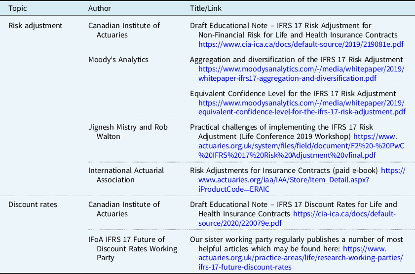
Disclaimer: The views expressed in this publication are those of invited contributors and not necessarily those of the Institute and Faculty of Actuaries. The Institute and Faculty of Actuaries do not endorse any of the views stated, nor any claims or representations made in this publication and accept no responsibility or liability to any person for loss or damage suffered as a consequence of their placing reliance upon any view, claim or representation made in this publication. The information and expressions of opinion contained in this publication are not intended to be a comprehensive study, nor to provide actuarial advice or advice of any nature and should not be treated as a substitute for specific advice concerning individual situations. On no account may any part of this publication be reproduced without the written permission of the Institute and Faculty of Actuaries.


 Open access