


1 Introduction
Increasingly stringent emissions regulations have prompted gas turbine manufacturers to switch to lean premixed combustion, but doing so provokes thermoacoustic instability (Lieuwen & Yang Reference Lieuwen and Yang2005). This phenomenon arises from positive coupling between the heat-release-rate (HRR) oscillations of an unsteady flame and one or more of the natural acoustic modes of the combustion chamber (Culick Reference Culick2006). If the HRR oscillations are sufficiently in phase with the acoustic pressure oscillations, the former can transfer energy to the latter via the Rayleigh (Reference Rayleigh1878) mechanism, resulting in high-amplitude self-excited flow oscillations at the characteristic acoustic frequencies of the system (Candel Reference Candel2002). If left unchecked, such thermoacoustic oscillations can reduce flame stability and increase thermal stresses (Lieuwen & Yang Reference Lieuwen and Yang2005). It is thus important to be able to control thermoacoustic oscillations in combustion systems (Poinsot Reference Poinsot2017).
1.1 Quasiperiodicity in self-excited thermoacoustic systems
Both passive and active methods are available to control thermoacoustic oscillations (Candel Reference Candel2002; Lieuwen & Yang Reference Lieuwen and Yang2005), but most assume a priori that such oscillations are periodic with a single characteristic frequency and a time-independent amplitude, i.e. they assume period-1 limit cycles (Kashinath, Li & Juniper Reference Kashinath, Li and Juniper2018). This assumption, however, is not always valid (Juniper & Sujith Reference Juniper and Sujith2018). Even early on, time-domain simulations by Jahnke & Culick (Reference Jahnke and Culick1994) have shown that a combustor with multiple acoustic modes can undergo a Neimark–Sacker (torus-birth) bifurcation to quasiperiodicity. In nonlinear dynamical systems, quasiperiodicity is a common state arising from interactions between at least two periodic modes whose natural frequencies, $f_{1}$
and
$f_{1}$
and $f_{2}$
, are incommensurate, i.e. their winding number,
$f_{2}$
, are incommensurate, i.e. their winding number, $f_{2}/f_{1}$
, is irrational. A two-frequency quasiperiodic system thus oscillates with a period of infinity and evolves in phase space along a non-repeating orbit on a
$f_{2}/f_{1}$
, is irrational. A two-frequency quasiperiodic system thus oscillates with a period of infinity and evolves in phase space along a non-repeating orbit on a $\mathbb{T}^{2}$
(two-dimensional) torus attractor formed by modes at
$\mathbb{T}^{2}$
(two-dimensional) torus attractor formed by modes at $f_{1}$
and
$f_{1}$
and $f_{2}$
(Thompson & Stewart Reference Thompson and Stewart2002).
$f_{2}$
(Thompson & Stewart Reference Thompson and Stewart2002).
Those early simulations by Jahnke & Culick (Reference Jahnke and Culick1994) have since been joined by numerous laboratory experiments showing similarly aperiodic dynamics. For example, Kabiraj et al. (Reference Kabiraj, Saurabh, Wahi and Sujith2012a
), Kabiraj, Sujith & Wahi (Reference Kabiraj, Sujith and Wahi2012b
) and Kabiraj & Sujith (Reference Kabiraj and Sujith2012) have shown that even a simple thermoacoustic system (a tube containing laminar premixed flames) can undergo a bifurcation cascade as a control parameter (the flame position within the tube) is varied, producing not just period-1 limit cycles, but also period- $k$
, frequency-locked, intermittent, chaotic and quasiperiodic oscillations. Later, Kashinath, Waugh & Juniper (Reference Kashinath, Waugh and Juniper2014) were able to reproduce these experimental findings, including quasiperiodicity, using low-order simulations of a
$k$
, frequency-locked, intermittent, chaotic and quasiperiodic oscillations. Later, Kashinath, Waugh & Juniper (Reference Kashinath, Waugh and Juniper2014) were able to reproduce these experimental findings, including quasiperiodicity, using low-order simulations of a $G$
-equation-based laminar premixed flame coupled with Galerkin acoustics. This has been followed by further experimental evidence of quasiperiodicity in both laminar (Vishnu, Sujith & Aghalayam Reference Vishnu, Sujith and Aghalayam2015) and turbulent (Gotoda et al.
Reference Gotoda, Okuno, Hayashi and Tachibana2015) systems. However, despite this growing evidence of quasiperiodic oscillations appearing in a variety of self-excited thermoacoustic systems, the control and suppression of such oscillations remain largely unexplored.
$G$
-equation-based laminar premixed flame coupled with Galerkin acoustics. This has been followed by further experimental evidence of quasiperiodicity in both laminar (Vishnu, Sujith & Aghalayam Reference Vishnu, Sujith and Aghalayam2015) and turbulent (Gotoda et al.
Reference Gotoda, Okuno, Hayashi and Tachibana2015) systems. However, despite this growing evidence of quasiperiodic oscillations appearing in a variety of self-excited thermoacoustic systems, the control and suppression of such oscillations remain largely unexplored.
1.2 Forced synchronization of periodic oscillations
Unlike quasiperiodic oscillations, periodic oscillations have been the subject of various control strategies in thermoacoustics, ranging from passive methods (Lieuwen Reference Lieuwen2003; Noiray et al. Reference Noiray, Durox, Schuller and Candel2009) to active methods (Heckl Reference Heckl1988; Dowling & Morgans Reference Dowling and Morgans2005; Bothien, Moeck & Paschereit Reference Bothien, Moeck and Paschereit2008). The simplest form of the latter is open-loop control, which requires only a single actuator (e.g. a fuel solenoid valve or a loudspeaker; McManus, Vandsburger & Bowman Reference McManus, Vandsburger and Bowman1990; Lubarsky et al. Reference Lubarsky, Shcherbik, Bibik and Zinn2003) and no sensors or feedback controllers, whose reliability can be questionable under the severe operating conditions of most combustors (Mongia et al. Reference Mongia, Held, Hsiao and Pandalai2003).
A versatile way to study open-loop control is in the framework of forced synchronization (Pikovsky, Rosenblum & Kurths Reference Pikovsky, Rosenblum and Kurths2003). In forced synchronization, a self-excited system oscillating at one or more of its natural frequencies is externally forced to oscillate at a different frequency (Balanov et al. Reference Balanov, Janson, Postnov and Sosnovtseva2008). This nonlinear process has been studied in many natural and technological systems (e.g. circadian rhythms and optical lasers; Glass Reference Glass2001; Boccaletti et al. Reference Boccaletti, Allaria, Meucci and Arecchi2002) and has been modelled with low-order universal oscillators such as the forced van der Pol (Reference van der Pol1927) (VDP) oscillator. The use of open-loop forcing to control self-excited oscillations has been gaining attention owing to its potential application in fields as diverse as optoelectronics, psychophysics and hydrodynamics (Hovel Reference Hovel2010).
In thermoacoustics, open-loop forcing has been shown to be able to weaken periodic self-excited oscillations in various combustion systems, ranging from the simple Rijke tube (Reynolds numbers of $Re\sim 10^{3}$
with natural frequencies of
$Re\sim 10^{3}$
with natural frequencies of $f_{1}\sim 10^{2}$
Hz; Guan, Murugesan & Li Reference Guan, Murugesan and Li2018; Kashinath et al.
Reference Kashinath, Li and Juniper2018; Guan et al.
Reference Guan, Gupta, Kashinath and Li2019a
; Mondal, Pawar & Sujith Reference Mondal, Pawar and Sujith2019) to turbulent premixed combustors (
$f_{1}\sim 10^{2}$
Hz; Guan, Murugesan & Li Reference Guan, Murugesan and Li2018; Kashinath et al.
Reference Kashinath, Li and Juniper2018; Guan et al.
Reference Guan, Gupta, Kashinath and Li2019a
; Mondal, Pawar & Sujith Reference Mondal, Pawar and Sujith2019) to turbulent premixed combustors ( $Re\sim 10^{4}$
,
$Re\sim 10^{4}$
, $f_{1}\sim 10^{2}$
Hz; Bellows, Hreiz & Lieuwen Reference Bellows, Hreiz and Lieuwen2008; Balusamy et al.
Reference Balusamy, Li, Han, Juniper and Hochgreb2015). A recurring theme of these studies has been the application of periodic acoustic forcing to periodic thermoacoustic oscillations, accompanied by an examination of the nonlinear dynamics en route to and beyond the synchronization boundaries. For example, on applying periodic acoustic forcing at an off-resonance frequency to a periodically oscillating laminar premixed flame in a tube, Guan et al. (Reference Guan, Gupta, Kashinath and Li2019a
) found: (i) a transition from unforced periodicity to
$f_{1}\sim 10^{2}$
Hz; Bellows, Hreiz & Lieuwen Reference Bellows, Hreiz and Lieuwen2008; Balusamy et al.
Reference Balusamy, Li, Han, Juniper and Hochgreb2015). A recurring theme of these studies has been the application of periodic acoustic forcing to periodic thermoacoustic oscillations, accompanied by an examination of the nonlinear dynamics en route to and beyond the synchronization boundaries. For example, on applying periodic acoustic forcing at an off-resonance frequency to a periodically oscillating laminar premixed flame in a tube, Guan et al. (Reference Guan, Gupta, Kashinath and Li2019a
) found: (i) a transition from unforced periodicity to $\mathbb{T}^{2}$
quasiperiodicity via a Neimark–Sacker bifurcation; (ii) a subsequent transition from
$\mathbb{T}^{2}$
quasiperiodicity via a Neimark–Sacker bifurcation; (ii) a subsequent transition from $\mathbb{T}^{2}$
quasiperiodicity to 1 : 1 synchronization at a critical forcing amplitude; (iii) a
$\mathbb{T}^{2}$
quasiperiodicity to 1 : 1 synchronization at a critical forcing amplitude; (iii) a $\vee$
-shaped Arnold tongue centred on the natural frequency; (iv) two different routes to synchronization, one via a saddle-node bifurcation and one via an inverse Neimark–Sacker bifurcation; and (v) that all of these dynamics could be qualitatively reproduced with a low-order universal oscillator containing a VDP kernel. Balusamy et al. (Reference Balusamy, Li, Han, Juniper and Hochgreb2015) applied similar off-resonance forcing to a swirl-stabilized turbulent premixed combustor and found additional synchronization dynamics, such as frequency pushing and pulling as well as phase locking, slipping, drifting and trapping – the latter a partially synchronous feature defined by frequency locking without phase locking (Li & Juniper Reference Li and Juniper2013c
). For high forcing amplitudes, Guan et al. (Reference Guan, Murugesan and Li2018) found that a synchronized system can transition out of synchronization and into strange non-chaotic and chaotic states, behaving in line with the Afraimovich & Shilnikov (Reference Afraimovich and Shilnikov1991) theorem for the collapse of a phase-locked torus.
$\vee$
-shaped Arnold tongue centred on the natural frequency; (iv) two different routes to synchronization, one via a saddle-node bifurcation and one via an inverse Neimark–Sacker bifurcation; and (v) that all of these dynamics could be qualitatively reproduced with a low-order universal oscillator containing a VDP kernel. Balusamy et al. (Reference Balusamy, Li, Han, Juniper and Hochgreb2015) applied similar off-resonance forcing to a swirl-stabilized turbulent premixed combustor and found additional synchronization dynamics, such as frequency pushing and pulling as well as phase locking, slipping, drifting and trapping – the latter a partially synchronous feature defined by frequency locking without phase locking (Li & Juniper Reference Li and Juniper2013c
). For high forcing amplitudes, Guan et al. (Reference Guan, Murugesan and Li2018) found that a synchronized system can transition out of synchronization and into strange non-chaotic and chaotic states, behaving in line with the Afraimovich & Shilnikov (Reference Afraimovich and Shilnikov1991) theorem for the collapse of a phase-locked torus.
From a control perspective, numerous studies have shown that, near the onset of synchronization, the thermoacoustic amplitude can be drastically reduced – typically to less than 20 % of that of the unforced state (Bellows et al. Reference Bellows, Hreiz and Lieuwen2008; Kashinath et al. Reference Kashinath, Li and Juniper2018; Guan et al. Reference Guan, Gupta, Kashinath and Li2019a ,Reference Guan, He, Murugesan, Li, Liu and Li b ; Mondal et al. Reference Mondal, Pawar and Sujith2019). This reduction occurs via asynchronous quenching, a nonlinear process in which the amplitude of a self-excited oscillator is reduced by the external application of periodic forcing at a frequency far enough from the natural frequency to prevent resonant amplification of the forcing signal (Minorsky Reference Minorsky1967). Asynchronous quenching can be modelled with a forced VDP oscillator (Dewan Reference Dewan1972) and has been exploited for open-loop control in various fields, ranging from plasma physics (Keen & Fletcher Reference Keen and Fletcher1970) to hydrodynamics (Staubli Reference Staubli1987). In thermoacoustics, asynchronous quenching has recently been shown to coincide with an inverse Neimark–Sacker bifurcation to synchronization and a reduced Rayleigh index (Guan et al. Reference Guan, Gupta, Kashinath and Li2019a ; Mondal et al. Reference Mondal, Pawar and Sujith2019). However, it is not known how effective this control strategy would be if it were applied to thermoacoustic oscillations that are quasiperiodic rather than periodic. Specifically, it is not known how the strategy would have to be modified to cope with the presence of an additional (second) natural mode. For example, in the periodic case, the thermoacoustic amplitude can be reduced by applying forcing at a frequency sufficiently far from the natural frequency for asynchronous quenching to occur, as demonstrated by Guan et al. (Reference Guan, Gupta, Kashinath and Li2019a ) and Mondal et al. (Reference Mondal, Pawar and Sujith2019). However, if a second natural mode is present, its frequency could coincide with the forcing frequency, resulting in resonant amplification (Minorsky Reference Minorsky1967). A potential way to avoid such amplification is to ensure that the forcing frequency is sufficiently far from both natural frequencies for asynchronous quenching to occur in both natural modes. However, this assumes that the two natural modes are similar in strength, which is not always the case in practice. As we will see in § 3, when one natural mode is significantly weaker than the other, it is possible to reduce the overall thermoacoustic amplitude by applying forcing at a frequency around the weaker natural mode and exploiting the same suppression mechanism (asynchronous quenching) as in the periodic case, albeit in more steps.
1.3 Forced synchronization of quasiperiodic oscillations
Two primary types of phase trajectories can exist on a two-frequency quasiperiodic attractor: a resonant limit cycle or an ergodic $\mathbb{T}^{2}$
torus (Balanov et al.
Reference Balanov, Janson, Postnov and Sosnovtseva2008). The former arises when the two natural modes are mutually synchronized such that their frequencies are commensurate, resulting in a phase trajectory that evolves along a closed periodic orbit on the quasiperiodic attractor. The latter arises when the two natural modes are not mutually synchronized and hence their frequencies are not commensurate, resulting in a phase trajectory that spirals non-repeatedly through every point on the quasiperiodic attractor. In this study, we focus on the forced synchronization of the latter type of solution. However, both types are reviewed here because they are closely related to each other.
$\mathbb{T}^{2}$
torus (Balanov et al.
Reference Balanov, Janson, Postnov and Sosnovtseva2008). The former arises when the two natural modes are mutually synchronized such that their frequencies are commensurate, resulting in a phase trajectory that evolves along a closed periodic orbit on the quasiperiodic attractor. The latter arises when the two natural modes are not mutually synchronized and hence their frequencies are not commensurate, resulting in a phase trajectory that spirals non-repeatedly through every point on the quasiperiodic attractor. In this study, we focus on the forced synchronization of the latter type of solution. However, both types are reviewed here because they are closely related to each other.
Anishchenko, Nikolaev & Kurths (Reference Anishchenko, Nikolaev and Kurths2007, Reference Anishchenko, Nikolaev and Kurths2008) have examined the effect of external forcing on a resonant limit cycle residing on a $\mathbb{T}^{2}$
torus. They used both (i) numerical simulations of an autonomous quasiperiodic oscillator – which was modelled as two coupled VDP oscillators – with two natural modes,
$\mathbb{T}^{2}$
torus. They used both (i) numerical simulations of an autonomous quasiperiodic oscillator – which was modelled as two coupled VDP oscillators – with two natural modes, $f_{1}$
and
$f_{1}$
and $f_{2}$
, undergoing mutual synchronization and subjected to sinusoidal forcing and (ii) laboratory experiments on an electronic circuit representing that oscillator. Those researchers found that the resonant limit cycle could generally be synchronized with the forcing. By analysing their data with Lyapunov exponents and Poincaré maps, they were able to identify the following four distinct states as the forcing amplitude increased at an off-resonance frequency,
$f_{2}$
, undergoing mutual synchronization and subjected to sinusoidal forcing and (ii) laboratory experiments on an electronic circuit representing that oscillator. Those researchers found that the resonant limit cycle could generally be synchronized with the forcing. By analysing their data with Lyapunov exponents and Poincaré maps, they were able to identify the following four distinct states as the forcing amplitude increased at an off-resonance frequency, $f_{f}$
(figures 5 and 6 of Anishchenko et al.
Reference Anishchenko, Nikolaev and Kurths2008).
$f_{f}$
(figures 5 and 6 of Anishchenko et al.
Reference Anishchenko, Nikolaev and Kurths2008).
(A) The $f_{f}$
mode is introduced, but mutual synchronization of
$f_{f}$
mode is introduced, but mutual synchronization of $f_{1}$
and
$f_{1}$
and $f_{2}$
continues, causing the resonant limit cycle to give way to a resonant
$f_{2}$
continues, causing the resonant limit cycle to give way to a resonant $\mathbb{T}_{f,1=2}^{2}$
torus at
$\mathbb{T}_{f,1=2}^{2}$
torus at $f_{f}$
and
$f_{f}$
and $f_{1}=f_{2}$
.
$f_{1}=f_{2}$
.
(B) Mutual synchronization no longer occurs, allowing $f_{1}$
and
$f_{1}$
and $f_{2}$
to assume different values, causing the resonant
$f_{2}$
to assume different values, causing the resonant $\mathbb{T}_{f,1=2}^{2}$
torus to give way to an ergodic
$\mathbb{T}_{f,1=2}^{2}$
torus to give way to an ergodic $\mathbb{T}_{f,1,2}^{3}$
torus with three incommensurate modes:
$\mathbb{T}_{f,1,2}^{3}$
torus with three incommensurate modes: $f_{f}$
,
$f_{f}$
, $f_{1}$
and
$f_{1}$
and $f_{2}$
. As
$f_{2}$
. As $f_{f}$
varies, different partial resonances can occur on the
$f_{f}$
varies, different partial resonances can occur on the $\mathbb{T}_{f,1,2}^{3}$
torus, leading to other
$\mathbb{T}_{f,1,2}^{3}$
torus, leading to other $\mathbb{T}^{2}$
quasiperiodic and chaotic states (Stankevich, Kurths & Kuznetsov Reference Stankevich, Kurths and Kuznetsov2015).
$\mathbb{T}^{2}$
quasiperiodic and chaotic states (Stankevich, Kurths & Kuznetsov Reference Stankevich, Kurths and Kuznetsov2015).
(C) Partial synchronization occurs, in which one of the natural modes synchronizes with the forcing ( $f_{2}=f_{f}$
), while the other remains desynchronized (
$f_{2}=f_{f}$
), while the other remains desynchronized ( $f_{1}\neq f_{f}$
). This leads to the emergence of a resonant
$f_{1}\neq f_{f}$
). This leads to the emergence of a resonant $\mathbb{T}_{f=2,1}^{2}$
torus on the existing
$\mathbb{T}_{f=2,1}^{2}$
torus on the existing $\mathbb{T}_{f,1,2}^{3}$
torus.
$\mathbb{T}_{f,1,2}^{3}$
torus.
(D) Complete synchronization occurs, in which both natural modes synchronize with the forcing ( $f_{f}=f_{1}=f_{2}$
), producing a period-1 limit cycle at
$f_{f}=f_{1}=f_{2}$
), producing a period-1 limit cycle at $f_{f}$
, as denoted by
$f_{f}$
, as denoted by $P1_{f}$
. In the literature, the term ‘complete synchronization’ is sometimes used to refer to the suppression of signal differences between two or more identical coupled chaotic oscillators (Pikovsky et al.
Reference Pikovsky, Rosenblum and Kurths2003). In this study, however, we follow the convention of Anishchenko et al. (Reference Anishchenko, Nikolaev and Kurths2008) by using this term to refer to the forced synchronization of the natural modes of a
$P1_{f}$
. In the literature, the term ‘complete synchronization’ is sometimes used to refer to the suppression of signal differences between two or more identical coupled chaotic oscillators (Pikovsky et al.
Reference Pikovsky, Rosenblum and Kurths2003). In this study, however, we follow the convention of Anishchenko et al. (Reference Anishchenko, Nikolaev and Kurths2008) by using this term to refer to the forced synchronization of the natural modes of a $\mathbb{T}^{2}$
quasiperiodic oscillator.
$\mathbb{T}^{2}$
quasiperiodic oscillator.
As mentioned earlier, a quasiperiodic attractor can also host an ergodic $\mathbb{T}^{2}$
torus. Loose, Wünsche & Henneberger (Reference Loose, Wünsche and Henneberger2010) have experimentally investigated the forced synchronization of such a torus using semiconductor lasers. They found similar states to those reported by Anishchenko et al. (Reference Anishchenko, Nikolaev and Kurths2007, Reference Anishchenko, Nikolaev and Kurths2008) (see above), with the exception that state (A) was bypassed because the two natural modes were not mutually synchronized at zero or low forcing amplitudes. Crucially, they also validated the VDP-oscillator predictions from Anishchenko et al. (Reference Anishchenko, Nikolaev and Kurths2007, Reference Anishchenko, Nikolaev and Kurths2008), showing that weak internal coupling leads to the partial synchronization of only one natural mode, but that strong internal coupling leads to the complete synchronization of both natural modes in succession. This qualitative agreement between complex experiments and simple phenomenological modelling provides compelling arguments for the universality of such synchronization phenomena (Loose et al.
Reference Loose, Wünsche and Henneberger2010).
$\mathbb{T}^{2}$
torus. Loose, Wünsche & Henneberger (Reference Loose, Wünsche and Henneberger2010) have experimentally investigated the forced synchronization of such a torus using semiconductor lasers. They found similar states to those reported by Anishchenko et al. (Reference Anishchenko, Nikolaev and Kurths2007, Reference Anishchenko, Nikolaev and Kurths2008) (see above), with the exception that state (A) was bypassed because the two natural modes were not mutually synchronized at zero or low forcing amplitudes. Crucially, they also validated the VDP-oscillator predictions from Anishchenko et al. (Reference Anishchenko, Nikolaev and Kurths2007, Reference Anishchenko, Nikolaev and Kurths2008), showing that weak internal coupling leads to the partial synchronization of only one natural mode, but that strong internal coupling leads to the complete synchronization of both natural modes in succession. This qualitative agreement between complex experiments and simple phenomenological modelling provides compelling arguments for the universality of such synchronization phenomena (Loose et al.
Reference Loose, Wünsche and Henneberger2010).
In thermoacoustics, only one study has previously examined the forced synchronization of an ergodic $\mathbb{T}^{2}$
torus. Using low-order simulations of a ducted laminar premixed flame, Kashinath et al. (Reference Kashinath, Li and Juniper2018) showed that applying periodic acoustic forcing at the dominant frequency of an ergodic
$\mathbb{T}^{2}$
torus. Using low-order simulations of a ducted laminar premixed flame, Kashinath et al. (Reference Kashinath, Li and Juniper2018) showed that applying periodic acoustic forcing at the dominant frequency of an ergodic $\mathbb{T}^{2}$
torus can cause it to completely synchronize with the forcing. However, because only one resonant value of
$\mathbb{T}^{2}$
torus can cause it to completely synchronize with the forcing. However, because only one resonant value of $f_{f}$
was used, neither the partial/complete synchronization boundaries nor the regimes of asynchronous quenching could be explored.
$f_{f}$
was used, neither the partial/complete synchronization boundaries nor the regimes of asynchronous quenching could be explored.
1.4 Contributions of this study
In this study, we take a synchronization approach to answering three research questions on the open-loop control of ergodic $\mathbb{T}^{2}$
quasiperiodic thermoacoustic oscillations.
$\mathbb{T}^{2}$
quasiperiodic thermoacoustic oscillations.
(i) Previous studies have shown that periodic acoustic forcing can control periodic thermoacoustic oscillations (§ 1.2), but can it also control quasiperiodic thermoacoustic oscillations? If it can, how does the synchronization process differ from that of the classical period-1 case studied by Guan et al. (Reference Guan, Gupta, Kashinath and Li2019a ) and Mondal et al. (Reference Mondal, Pawar and Sujith2019)?
(ii) If periodic acoustic forcing can control quasiperiodic thermoacoustic oscillations, what are the optimal forcing conditions for producing the maximum reduction in thermoacoustic amplitude? It is necessary to know this if one is to fully exploit synchronization phenomena, such as asynchronous quenching (§ 1.2), for open-loop control.
(iii) Previous studies on electronic circuits and semiconductor lasers have shown that the forced synchronization of quasiperiodic oscillations can be qualitatively modelled with low-order universal oscillators containing a VDP kernel (§ 1.3), but can such a phenomenological modelling approach work on thermoacoustic systems as well? In other words, can the forced synchronization of quasiperiodic thermoacoustic oscillations – particularly the partial/complete synchronization boundaries and asynchronous quenching – be qualitatively modelled with just two coupled VDP oscillators forced by a sinusoidal term? If so, this would strengthen the universality of synchronization in physically disparate systems and open up new possibilities for the development of active control strategies in thermoacoustic systems with multiple time scales.
To answer these questions, we perform experiments on a prototypical thermoacoustic system (§ 2) that is known to exhibit a variety of nonlinear self-excited states, including ergodic $\mathbb{T}^{2}$
quasiperiodicity. We acoustically force this system around its two natural frequencies, at varying amplitudes, and measure its pressure and HRR response. By analysing the data within a synchronization framework, we find that the forcing can weaken
$\mathbb{T}^{2}$
quasiperiodicity. We acoustically force this system around its two natural frequencies, at varying amplitudes, and measure its pressure and HRR response. By analysing the data within a synchronization framework, we find that the forcing can weaken $\mathbb{T}^{2}$
quasiperiodic thermoacoustic oscillations – via the sequential birth of partially and completely synchronous states – if the forcing frequency and amplitude are appropriately chosen (§ 3). We then show that these dynamics can be qualitatively reproduced with two coupled VDP oscillators forced by a sinusoidal term (§ 4). We conclude this paper by discussing the implications and limitations of these findings (§ 5).
$\mathbb{T}^{2}$
quasiperiodic thermoacoustic oscillations – via the sequential birth of partially and completely synchronous states – if the forcing frequency and amplitude are appropriately chosen (§ 3). We then show that these dynamics can be qualitatively reproduced with two coupled VDP oscillators forced by a sinusoidal term (§ 4). We conclude this paper by discussing the implications and limitations of these findings (§ 5).
2 Experimental set-up and data analysis
The prototypical thermoacoustic system under study consists of a laminar conical premixed flame in a tube combustor subjected to external acoustic forcing. Figure 1 shows the experimental set-up, which is identical to that of our recent studies on periodic thermoacoustic oscillations (Guan et al.
Reference Guan, Murugesan and Li2018, Reference Guan, Gupta, Kashinath and Li2019a
,Reference Guan, He, Murugesan, Li, Liu and Li
b
) and which is modelled after the numerical set-up of Kashinath et al. (Reference Kashinath, Li and Juniper2018). The system has four main components: a stainless steel burner (inner diameter, ID: 16.8 mm; length: 800 mm), a quartz tube combustor with double open ends (ID: 44 mm; length: $L=860$
mm), an acoustic decoupler (ID: 180 mm; length: 200 mm) and a loudspeaker for acoustic forcing. A copper extension tip (ID:
$L=860$
mm), an acoustic decoupler (ID: 180 mm; length: 200 mm) and a loudspeaker for acoustic forcing. A copper extension tip (ID: $D=12$
mm; length: 30 mm) containing a fine-mesh screen is mounted at the burner exit for improved flame stability. The flame is created from a premixed mixture of air and liquefied petroleum gas (LPG: 70 % butane, 30 % propane). The flow rate of the LPG is metered with a rotameter (
$D=12$
mm; length: 30 mm) containing a fine-mesh screen is mounted at the burner exit for improved flame stability. The flame is created from a premixed mixture of air and liquefied petroleum gas (LPG: 70 % butane, 30 % propane). The flow rate of the LPG is metered with a rotameter ( $\pm 2.5\,\%$
), while that of the air is metered with a mass flow controller (Alicat MCR Series:
$\pm 2.5\,\%$
), while that of the air is metered with a mass flow controller (Alicat MCR Series: $\pm 0.2\,\%$
). The two reactants are then brought together in a mixing chamber before being piped to the burner.
$\pm 0.2\,\%$
). The two reactants are then brought together in a mixing chamber before being piped to the burner.

Figure 1. Diagram of the experimental set-up, whose main components include a stainless steel burner, a copper burner extension (see inset), a quartz tube combustor with double open ends, an acoustic decoupler, a loudspeaker and a motorized linear traverse for adjusting the flame position ( $\tilde{z}\equiv z/L$
) within the combustor. The key dimensions of these components are stated in the text. The measurement diagnostics include two probe microphones (PM-1, PM-2) for the acoustic pressure in the combustor, a hot-wire probe (not shown) for the acoustic velocity perturbation at the burner exit, a photomultiplier tube (PMT) for the global CH* chemiluminescence from the flame and a high-speed camera (HSC) for time-resolved flame imaging. All dimensions shown are in millimetres. The diagram is not drawn to scale.
$\tilde{z}\equiv z/L$
) within the combustor. The key dimensions of these components are stated in the text. The measurement diagnostics include two probe microphones (PM-1, PM-2) for the acoustic pressure in the combustor, a hot-wire probe (not shown) for the acoustic velocity perturbation at the burner exit, a photomultiplier tube (PMT) for the global CH* chemiluminescence from the flame and a high-speed camera (HSC) for time-resolved flame imaging. All dimensions shown are in millimetres. The diagram is not drawn to scale.
When unforced, this thermoacoustic system can exhibit a variety of nonlinear self-excited states – including period-1 limit cycles, quasiperiodicity and chaos – depending on the equivalence ratio and the flame position within the combustor (Guan et al.
Reference Guan, Murugesan and Li2018, Reference Guan, Gupta, Kashinath and Li2019a
,Reference Guan, He, Murugesan, Li, Liu and Li
b
). As this study focuses on the open-loop control of ergodic $\mathbb{T}^{2}$
quasiperiodic oscillations (§ 1.4), we apply forcing to a quasiperiodic state containing two incommensurate natural frequencies:
$\mathbb{T}^{2}$
quasiperiodic oscillations (§ 1.4), we apply forcing to a quasiperiodic state containing two incommensurate natural frequencies: $f_{1}$
and
$f_{1}$
and $f_{2}$
. The details of this state will be examined in § 3.1.
$f_{2}$
. The details of this state will be examined in § 3.1.
To generate the forcing, we use a loudspeaker (FaitalPRO 6FE100) mounted in the acoustic decoupler (figure 1) and driven by a power amplifier (Alesis RA150) controlled by a digital function generator (Keysight 33512B) with a sinusoidal output. We apply the forcing across a range of amplitudes (up to flame blow-off) and frequencies ( $0.60\leqslant f_{f}/f_{1}\leqslant 1.20$
;
$0.60\leqslant f_{f}/f_{1}\leqslant 1.20$
; $0.86\leqslant f_{f}/f_{2}\leqslant 1.71$
) so as to explore the full synchronization dynamics around both
$0.86\leqslant f_{f}/f_{2}\leqslant 1.71$
) so as to explore the full synchronization dynamics around both $f_{1}$
and
$f_{1}$
and $f_{2}$
. We define the forcing amplitude as the velocity perturbation amplitude at the burner exit normalized by the time-averaged velocity of the bulk reactants:
$f_{2}$
. We define the forcing amplitude as the velocity perturbation amplitude at the burner exit normalized by the time-averaged velocity of the bulk reactants: $\unicode[STIX]{x1D716}_{f}\equiv |u^{\prime }|/\bar{u}$
. We measure
$\unicode[STIX]{x1D716}_{f}\equiv |u^{\prime }|/\bar{u}$
. We measure $|u^{\prime }|$
with a hot-wire anemometer (Dantec MiniCTA with a
$|u^{\prime }|$
with a hot-wire anemometer (Dantec MiniCTA with a $5~\unicode[STIX]{x03BC}\text{m}$
diameter tungsten probe) operating in constant temperature mode and calibrated to an uncertainty of
$5~\unicode[STIX]{x03BC}\text{m}$
diameter tungsten probe) operating in constant temperature mode and calibrated to an uncertainty of $\pm 1.3\,\%$
via the procedure of Johnson, Uddin & Pollard (Reference Johnson, Uddin and Pollard2005).
$\pm 1.3\,\%$
via the procedure of Johnson, Uddin & Pollard (Reference Johnson, Uddin and Pollard2005).
To characterize the synchronization dynamics and compute the Rayleigh index, we use simultaneous measurements of the acoustic pressure fluctuations in the combustor ( $p^{\prime }$
) and of the global HRR fluctuations from the flame (
$p^{\prime }$
) and of the global HRR fluctuations from the flame ( $q^{\prime }$
). We measure
$q^{\prime }$
). We measure $p^{\prime }(t)$
with two probe microphones (GRAS 40SA: sensitivity of
$p^{\prime }(t)$
with two probe microphones (GRAS 40SA: sensitivity of $3~\text{mV}~\text{Pa}^{-1}$
;
$3~\text{mV}~\text{Pa}^{-1}$
; $\pm 2.5\times 10^{-5}$
Pa) mounted 43 mm (PM-1) and 387 mm (PM-2) from the bottom of the combustor (figure 1). In most of our analyses, however, we use the
$\pm 2.5\times 10^{-5}$
Pa) mounted 43 mm (PM-1) and 387 mm (PM-2) from the bottom of the combustor (figure 1). In most of our analyses, however, we use the $p^{\prime }(t)$
signal from PM-2 because it behaves qualitatively similarly to that from PM-1 but has a higher signal-to-noise ratio and is located exactly at the flame position, which is important for computing the Rayleigh index. Before each test run, we calibrate both microphones against a certified sound source (Brüel & Kjær Type 4231). We measure
$p^{\prime }(t)$
signal from PM-2 because it behaves qualitatively similarly to that from PM-1 but has a higher signal-to-noise ratio and is located exactly at the flame position, which is important for computing the Rayleigh index. Before each test run, we calibrate both microphones against a certified sound source (Brüel & Kjær Type 4231). We measure $q^{\prime }(t)$
with a photomultiplier tube (PMT: Thorlabs PMM01;
$q^{\prime }(t)$
with a photomultiplier tube (PMT: Thorlabs PMM01; $\pm 1.5\,\%$
) viewing through a bandpass optical filter centred on 430 nm (10 nm bandwidth), thus capturing the CH* chemiluminescence emission from the flame (Gaydon Reference Gaydon1974). At each forcing condition, we digitize the voltage signals from the microphones and PMT at 16384 Hz for 6 s on a 16-bit data acquisition system (DAQ: NI USB-6356).
$\pm 1.5\,\%$
) viewing through a bandpass optical filter centred on 430 nm (10 nm bandwidth), thus capturing the CH* chemiluminescence emission from the flame (Gaydon Reference Gaydon1974). At each forcing condition, we digitize the voltage signals from the microphones and PMT at 16384 Hz for 6 s on a 16-bit data acquisition system (DAQ: NI USB-6356).
We process the data in several ways, including (i) in the frequency domain via the power spectral density (PSD), which is computed using the Welch (Reference Welch1967) algorithm, with Hamming windows to reduce spectral leakage, resulting in a frequency resolution of 0.5 Hz; (ii) via the complex analytic signal, which is computed with the Hilbert transform (Gabor Reference Gabor1946) and is used to determine the instantaneous phase difference between the forcing and the system, $\unicode[STIX]{x0394}\unicode[STIX]{x1D713}_{f,p^{\prime }}\equiv \unicode[STIX]{x1D713}_{f}-\unicode[STIX]{x1D713}_{p^{\prime }}$
; and (iii) in phase space via nonlinear time-series analysis (Kantz & Schreiber Reference Kantz and Schreiber2003). It should be cautioned that, when applied to an aperiodic signal with multiple different frequencies, the Hilbert transform can give physically undefined values of the instantaneous phase (Boashash Reference Boashash1992). This limitation, however, does not necessarily imply that the Hilbert transform cannot still provide useful insight into the forced synchronization of a system oscillating aperiodically (Pikovsky et al.
Reference Pikovsky, Rosenblum, Osipov and Kurths1997; Mondal, Pawar & Sujith Reference Mondal, Pawar and Sujith2017). In this study, we follow the convention of the synchronization community by taking a conservative approach whereby the results of the Hilbert transform are cross-checked against other independent synchronization indicators. For example, in nonlinear time-series analysis, we reconstruct the phase space using the embedding theorem of Takens (Reference Takens, Rand and Young1981). In this procedure, we determine (i) the optimal time delay (
$\unicode[STIX]{x0394}\unicode[STIX]{x1D713}_{f,p^{\prime }}\equiv \unicode[STIX]{x1D713}_{f}-\unicode[STIX]{x1D713}_{p^{\prime }}$
; and (iii) in phase space via nonlinear time-series analysis (Kantz & Schreiber Reference Kantz and Schreiber2003). It should be cautioned that, when applied to an aperiodic signal with multiple different frequencies, the Hilbert transform can give physically undefined values of the instantaneous phase (Boashash Reference Boashash1992). This limitation, however, does not necessarily imply that the Hilbert transform cannot still provide useful insight into the forced synchronization of a system oscillating aperiodically (Pikovsky et al.
Reference Pikovsky, Rosenblum, Osipov and Kurths1997; Mondal, Pawar & Sujith Reference Mondal, Pawar and Sujith2017). In this study, we follow the convention of the synchronization community by taking a conservative approach whereby the results of the Hilbert transform are cross-checked against other independent synchronization indicators. For example, in nonlinear time-series analysis, we reconstruct the phase space using the embedding theorem of Takens (Reference Takens, Rand and Young1981). In this procedure, we determine (i) the optimal time delay ( $\unicode[STIX]{x1D70F}$
) via the first local minimum of the average mutual information function (Fraser & Swinney Reference Fraser and Swinney1986) and (ii) the minimum embedding dimension (
$\unicode[STIX]{x1D70F}$
) via the first local minimum of the average mutual information function (Fraser & Swinney Reference Fraser and Swinney1986) and (ii) the minimum embedding dimension ( $d$
) via the method of Cao (Reference Cao1997). After reconstructing the phase space, we visualize the attractor (limit set) within it using three-dimensional phase portraits and one-sided Poincaré maps. To quantify the degree of topological self-similarity in the attractor, we compute its correlation dimension (
$d$
) via the method of Cao (Reference Cao1997). After reconstructing the phase space, we visualize the attractor (limit set) within it using three-dimensional phase portraits and one-sided Poincaré maps. To quantify the degree of topological self-similarity in the attractor, we compute its correlation dimension ( $\overline{D_{c}}$
) with the algorithm of Grassberger & Procaccia (Reference Grassberger and Procaccia1983). This is an invariant measure of the number of active degrees of freedom (DOFs) in a dynamical system and can be used to distinguish between a fixed point (
$\overline{D_{c}}$
) with the algorithm of Grassberger & Procaccia (Reference Grassberger and Procaccia1983). This is an invariant measure of the number of active degrees of freedom (DOFs) in a dynamical system and can be used to distinguish between a fixed point ( $\overline{D_{c}}=0$
), a periodic limit cycle (
$\overline{D_{c}}=0$
), a periodic limit cycle ( $\overline{D_{c}}=1$
), a
$\overline{D_{c}}=1$
), a $\mathbb{T}^{2}$
torus (
$\mathbb{T}^{2}$
torus ( $\overline{D_{c}}=2$
), a
$\overline{D_{c}}=2$
), a $\mathbb{T}^{3}$
torus (
$\mathbb{T}^{3}$
torus ( $\overline{D_{c}}=3$
) and a strange attractor (
$\overline{D_{c}}=3$
) and a strange attractor ( $\overline{D_{c}}=$
non-integer). For a detailed discussion of these methods, the reader is referred to the books by Kantz & Schreiber (Reference Kantz and Schreiber2003) and Small (Reference Small2005).
$\overline{D_{c}}=$
non-integer). For a detailed discussion of these methods, the reader is referred to the books by Kantz & Schreiber (Reference Kantz and Schreiber2003) and Small (Reference Small2005).
To complement the $p^{\prime }(t)$
and
$p^{\prime }(t)$
and $q^{\prime }(t)$
data, we capture time-resolved broadband chemiluminescence images of the flame with a high-speed camera (Phantom M310: dynamic range of 12 bits) operating at an image resolution of
$q^{\prime }(t)$
data, we capture time-resolved broadband chemiluminescence images of the flame with a high-speed camera (Phantom M310: dynamic range of 12 bits) operating at an image resolution of $512\times 512$
pixels and a frame rate of 3000 Hz. As § 3.1 will show, this frame rate is an order of magnitude higher than the highest natural frequency of the self-excited
$512\times 512$
pixels and a frame rate of 3000 Hz. As § 3.1 will show, this frame rate is an order of magnitude higher than the highest natural frequency of the self-excited $\mathbb{T}^{2}$
thermoacoustic oscillations (
$\mathbb{T}^{2}$
thermoacoustic oscillations ( $f_{1}=248\pm 1.5$
Hz), ensuring that the flame imaging is time resolved.
$f_{1}=248\pm 1.5$
Hz), ensuring that the flame imaging is time resolved.
3 Experimental results and discussion
3.1 Natural self-excited dynamics: ergodic $\mathbb{T}^{2}$
quasiperiodicity
$\mathbb{T}^{2}$
quasiperiodicity

Before examining the forced dynamics, it is necessary to find an unforced self-excited state with ergodic $\mathbb{T}^{2}$
quasiperiodicity at two incommensurate frequencies. In our system, such a state can be found at an equivalence ratio of
$\mathbb{T}^{2}$
quasiperiodicity at two incommensurate frequencies. In our system, such a state can be found at an equivalence ratio of $\unicode[STIX]{x1D719}=0.57$
(
$\unicode[STIX]{x1D719}=0.57$
( $\pm 3.2\,\%$
), a bulk reactant velocity of
$\pm 3.2\,\%$
), a bulk reactant velocity of $\bar{u}=1.58~\text{m}~\text{s}^{-1}$
(
$\bar{u}=1.58~\text{m}~\text{s}^{-1}$
( $\pm 0.2\,\%$
), a Reynolds number of
$\pm 0.2\,\%$
), a Reynolds number of $Re\equiv \unicode[STIX]{x1D70C}\bar{u}D/\unicode[STIX]{x1D707}=1280$
(
$Re\equiv \unicode[STIX]{x1D70C}\bar{u}D/\unicode[STIX]{x1D707}=1280$
( $\pm 1.7\,\%$
), where
$\pm 1.7\,\%$
), where $\unicode[STIX]{x1D70C}$
and
$\unicode[STIX]{x1D70C}$
and $\unicode[STIX]{x1D707}$
are the density and dynamic viscosity of the reactants, and a flame position of
$\unicode[STIX]{x1D707}$
are the density and dynamic viscosity of the reactants, and a flame position of $\tilde{z}\equiv z/L=0.45$
(
$\tilde{z}\equiv z/L=0.45$
( $\pm 0.4\,\%$
), where
$\pm 0.4\,\%$
), where $z$
is the distance between the burner extension tip and the bottom of the combustor (figure 1). To consolidate the discussion, we present results mostly from this operating condition, but note that its synchronization dynamics (e.g. its bifurcations, synchronous states and Arnold tongues) are qualitatively representative of a range of operating conditions in which
$z$
is the distance between the burner extension tip and the bottom of the combustor (figure 1). To consolidate the discussion, we present results mostly from this operating condition, but note that its synchronization dynamics (e.g. its bifurcations, synchronous states and Arnold tongues) are qualitatively representative of a range of operating conditions in which $\mathbb{T}^{2}$
quasiperiodicity occurs.
$\mathbb{T}^{2}$
quasiperiodicity occurs.
Figure 2. Natural self-excited dynamics of a thermoacoustic system undergoing ergodic $\mathbb{T}^{2}$
quasiperiodic oscillations: (a) time trace, (b) PSD, (c) phase portrait and Poincaré map and (d) slope of the correlation sum, all computed from the acoustic pressure fluctuations (
$\mathbb{T}^{2}$
quasiperiodic oscillations: (a) time trace, (b) PSD, (c) phase portrait and Poincaré map and (d) slope of the correlation sum, all computed from the acoustic pressure fluctuations ( $p^{\prime }$
from PM-2) in the combustor. In (c), phase-space reconstruction is performed with
$p^{\prime }$
from PM-2) in the combustor. In (c), phase-space reconstruction is performed with $d=3$
and
$d=3$
and $\unicode[STIX]{x1D70F}=0.005$
s. Panel (e) shows a sequence of time-resolved Abel-inverted images of the flame captured via broadband chemiluminescence (successive images are separated in time by
$\unicode[STIX]{x1D70F}=0.005$
s. Panel (e) shows a sequence of time-resolved Abel-inverted images of the flame captured via broadband chemiluminescence (successive images are separated in time by $1/1500$
s).
$1/1500$
s).
Figure 2 shows the natural self-excited dynamics at this operating condition. To establish the existence of ergodic $\mathbb{T}^{2}$
quasiperiodicity, we examine a variety of indicators, beginning with the (a) time trace, (b) PSD and (c) phase portrait and Poincaré map of the acoustic pressure fluctuations (
$\mathbb{T}^{2}$
quasiperiodicity, we examine a variety of indicators, beginning with the (a) time trace, (b) PSD and (c) phase portrait and Poincaré map of the acoustic pressure fluctuations ( $p^{\prime }$
from PM-2) in the combustor. The first indication that the system is quasiperiodic can be found in the PSD (figure 2
b), where a pair of sharp dominant peaks appears at two incommensurate natural frequencies:
$p^{\prime }$
from PM-2) in the combustor. The first indication that the system is quasiperiodic can be found in the PSD (figure 2
b), where a pair of sharp dominant peaks appears at two incommensurate natural frequencies: $f_{1}=248\pm 1.5$
and
$f_{1}=248\pm 1.5$
and $f_{2}=174\pm 1.5$
Hz. The peak at
$f_{2}=174\pm 1.5$
Hz. The peak at $f_{1}$
is nearly 20 dB (i.e. 10 times) higher than that at
$f_{1}$
is nearly 20 dB (i.e. 10 times) higher than that at $f_{2}$
, which, as we will see in § 3.2.3, has fundamental implications for the way in which the system transitions from partial to complete synchronization. Surrounding these two peaks (
$f_{2}$
, which, as we will see in § 3.2.3, has fundamental implications for the way in which the system transitions from partial to complete synchronization. Surrounding these two peaks ( $f_{1}$
and
$f_{1}$
and $f_{2}$
) are several weaker peaks at their linear combinations (
$f_{2}$
) are several weaker peaks at their linear combinations ( $|nf_{1}\pm mf_{2}|$
, where
$|nf_{1}\pm mf_{2}|$
, where $n$
and
$n$
and $m$
are integers), indicating the presence of nonlinear wave–triad interactions between the two natural modes (Schmid & Henningson Reference Schmid and Henningson2012). In the time trace (figure 2
a), these interactions give rise to amplitude modulations at a relatively low frequency of
$m$
are integers), indicating the presence of nonlinear wave–triad interactions between the two natural modes (Schmid & Henningson Reference Schmid and Henningson2012). In the time trace (figure 2
a), these interactions give rise to amplitude modulations at a relatively low frequency of $f=f_{1}-f_{2}\approx 74$
Hz. These beating modulations are a classical feature of self-excited oscillators with multiple natural modes (Pikovsky et al.
Reference Pikovsky, Rosenblum and Kurths2003) and have been observed in various quasiperiodic systems, including flame-driven combustors (Mondal et al.
Reference Mondal, Pawar and Sujith2017). The quasiperiodic nature of this system is also evident in its phase portrait (figure 2
c), where the phase trajectory can be seen evolving on a stable attractor with a toroidal topology, i.e. a torus attractor. In the Poincaré map (inset of figure 2
c), the intercepts of this trajectory form a closed continuous ring, indicating that the torus is ergodic with an irrational winding number (Hilborn Reference Hilborn2000).
$f=f_{1}-f_{2}\approx 74$
Hz. These beating modulations are a classical feature of self-excited oscillators with multiple natural modes (Pikovsky et al.
Reference Pikovsky, Rosenblum and Kurths2003) and have been observed in various quasiperiodic systems, including flame-driven combustors (Mondal et al.
Reference Mondal, Pawar and Sujith2017). The quasiperiodic nature of this system is also evident in its phase portrait (figure 2
c), where the phase trajectory can be seen evolving on a stable attractor with a toroidal topology, i.e. a torus attractor. In the Poincaré map (inset of figure 2
c), the intercepts of this trajectory form a closed continuous ring, indicating that the torus is ergodic with an irrational winding number (Hilborn Reference Hilborn2000).
To verify the two-dimensionality of the torus, we estimate its fractal dimension by computing $\overline{D_{c}}$
as per § 2. Figure 2(d) shows the local slope of the correlation sum (
$\overline{D_{c}}$
as per § 2. Figure 2(d) shows the local slope of the correlation sum ( $D_{c}=\unicode[STIX]{x2202}\log C_{N}/\unicode[STIX]{x2202}\log R$
) as a function of the normalized hypersphere radius (
$D_{c}=\unicode[STIX]{x2202}\log C_{N}/\unicode[STIX]{x2202}\log R$
) as a function of the normalized hypersphere radius ( $R/R_{max}$
) for three embedding dimensions (
$R/R_{max}$
) for three embedding dimensions ( $d=8$
, 10 and 12), all of which are high enough for
$d=8$
, 10 and 12), all of which are high enough for $D_{c}$
to converge. Within the self-similar Euclidean scaling range (
$D_{c}$
to converge. Within the self-similar Euclidean scaling range ( $10^{-2}\leqslant R/R_{max}\leqslant 10^{-1}$
),
$10^{-2}\leqslant R/R_{max}\leqslant 10^{-1}$
), $D_{c}$
converges to an average integer value of
$D_{c}$
converges to an average integer value of $\overline{D_{c}}\approx 2$
, confirming that the torus is indeed two-dimensional. This is consistent with our earlier observation of two incommensurate natural frequencies (
$\overline{D_{c}}\approx 2$
, confirming that the torus is indeed two-dimensional. This is consistent with our earlier observation of two incommensurate natural frequencies ( $f_{1}$
and
$f_{1}$
and $f_{2}$
) in the PSD (figure 2
b).
$f_{2}$
) in the PSD (figure 2
b).
To complement the pressure data, we show in figure 2(e) a sequence of time-resolved Abel-inverted images of the flame captured via broadband chemiluminescence emission (§ 2). If the system were simply oscillating in a periodic limit cycle at a dominant natural frequency of $f_{1}=248\pm 1.5$
Hz, then the image sequence, which is recorded at 3000 Hz, would repeat itself around once every 12 frames, i.e. at
$f_{1}=248\pm 1.5$
Hz, then the image sequence, which is recorded at 3000 Hz, would repeat itself around once every 12 frames, i.e. at $t_{1}$
,
$t_{1}$
, $t_{13}$
,
$t_{13}$
, $t_{25}$
and
$t_{25}$
and $t_{37}$
. However, as figure 2(e) shows, the flame contours at these four time instants (highlighted in yellow) are markedly different from each other, in accordance with our assessment that the system is exhibiting behaviour more complex than just a periodic limit cycle.
$t_{37}$
. However, as figure 2(e) shows, the flame contours at these four time instants (highlighted in yellow) are markedly different from each other, in accordance with our assessment that the system is exhibiting behaviour more complex than just a periodic limit cycle.
In summary, by examining $p^{\prime }(t)$
in the time, frequency and phase domains as well as by inspecting time-resolved Abel-inverted flame images, we have established that the natural self-excited dynamics of the system is quasiperiodic, with its phase trajectory evolving on a stable ergodic
$p^{\prime }(t)$
in the time, frequency and phase domains as well as by inspecting time-resolved Abel-inverted flame images, we have established that the natural self-excited dynamics of the system is quasiperiodic, with its phase trajectory evolving on a stable ergodic $\mathbb{T}^{2}$
torus attractor formed by two incommensurate natural modes:
$\mathbb{T}^{2}$
torus attractor formed by two incommensurate natural modes: $f_{1}$
and
$f_{1}$
and $f_{2}$
. From here onwards, we will refer to this self-excited state as
$f_{2}$
. From here onwards, we will refer to this self-excited state as $\mathbb{T}_{1,2}^{2}$
, with subscripts 1 and 2 denoting the dominant roles played by modes
$\mathbb{T}_{1,2}^{2}$
, with subscripts 1 and 2 denoting the dominant roles played by modes $f_{1}$
and
$f_{1}$
and $f_{2}$
.
$f_{2}$
.
3.2 Forced synchronization: period-1,
$\mathbb{T}^{2}$
and
$\mathbb{T}^{3}$
quasiperiodic states


Having established that the self-excited dynamics is dominated by ergodic $\mathbb{T}^{2}$
quasiperiodicity, we proceed to examine the forced synchronization dynamics. We begin with two synchronization maps, both in a parameter space defined by the forcing frequency (
$\mathbb{T}^{2}$
quasiperiodicity, we proceed to examine the forced synchronization dynamics. We begin with two synchronization maps, both in a parameter space defined by the forcing frequency ( $f_{f}/f_{1}$
or
$f_{f}/f_{1}$
or $f_{f}/f_{2}$
) and the forcing amplitude (
$f_{f}/f_{2}$
) and the forcing amplitude ( $\unicode[STIX]{x1D716}_{f}\equiv |u^{\prime }|/\bar{u}$
), but with one (figure 3
a) showing the forcing conditions at which different dynamical states arise and the other (figure 3
b) showing contours of the normalized response amplitude. The normalized response amplitude is defined as
$\unicode[STIX]{x1D716}_{f}\equiv |u^{\prime }|/\bar{u}$
), but with one (figure 3
a) showing the forcing conditions at which different dynamical states arise and the other (figure 3
b) showing contours of the normalized response amplitude. The normalized response amplitude is defined as $\unicode[STIX]{x1D702}_{p^{\prime }}\equiv (\unicode[STIX]{x1D70E}_{p^{\prime }}^{\ast }-\unicode[STIX]{x1D70E}_{p^{\prime }})/\unicode[STIX]{x1D70E}_{p^{\prime }}$
, where
$\unicode[STIX]{x1D702}_{p^{\prime }}\equiv (\unicode[STIX]{x1D70E}_{p^{\prime }}^{\ast }-\unicode[STIX]{x1D70E}_{p^{\prime }})/\unicode[STIX]{x1D70E}_{p^{\prime }}$
, where $\unicode[STIX]{x1D70E}_{p^{\prime }}^{\ast }$
and
$\unicode[STIX]{x1D70E}_{p^{\prime }}^{\ast }$
and $\unicode[STIX]{x1D70E}_{p^{\prime }}$
denote the root mean square of
$\unicode[STIX]{x1D70E}_{p^{\prime }}$
denote the root mean square of $p^{\prime }(t)$
when the system is forced and unforced, respectively. Consequently, the thermoacoustic oscillations are weakened by the forcing when
$p^{\prime }(t)$
when the system is forced and unforced, respectively. Consequently, the thermoacoustic oscillations are weakened by the forcing when $\unicode[STIX]{x1D702}_{p^{\prime }}<0$
(blue regions) but are amplified by the forcing when
$\unicode[STIX]{x1D702}_{p^{\prime }}<0$
(blue regions) but are amplified by the forcing when $\unicode[STIX]{x1D702}_{p^{\prime }}>0$
(red regions). Overlaid on the contours of
$\unicode[STIX]{x1D702}_{p^{\prime }}>0$
(red regions). Overlaid on the contours of $\unicode[STIX]{x1D702}_{p^{\prime }}$
(figure 3
b) are discrete markers showing the onset of complete synchronization for two different self-excited states: the
$\unicode[STIX]{x1D702}_{p^{\prime }}$
(figure 3
b) are discrete markers showing the onset of complete synchronization for two different self-excited states: the $\mathbb{T}_{1,2}^{2}$
state of the present study (white–red markers) and the period-1 state (
$\mathbb{T}_{1,2}^{2}$
state of the present study (white–red markers) and the period-1 state ( $P1_{1}$
) studied by Guan et al. (Reference Guan, Gupta, Kashinath and Li2019a
) (black markers). The latter is shown for comparison with the forced synchronization of a periodic limit cycle.
$P1_{1}$
) studied by Guan et al. (Reference Guan, Gupta, Kashinath and Li2019a
) (black markers). The latter is shown for comparison with the forced synchronization of a periodic limit cycle.

Figure 3. Forced response of an ergodic $\mathbb{T}_{1,2}^{2}$
thermoacoustic system: synchronization maps showing (a) the forcing conditions at which four different dynamical states arise and (b) contours of the normalized response amplitude (
$\mathbb{T}_{1,2}^{2}$
thermoacoustic system: synchronization maps showing (a) the forcing conditions at which four different dynamical states arise and (b) contours of the normalized response amplitude ( $\unicode[STIX]{x1D702}_{p^{\prime }}$
), both in a parameter space defined by the forcing frequency (
$\unicode[STIX]{x1D702}_{p^{\prime }}$
), both in a parameter space defined by the forcing frequency ( $f_{f}/f_{1}$
or
$f_{f}/f_{1}$
or $f_{f}/f_{2}$
) and the forcing amplitude (
$f_{f}/f_{2}$
) and the forcing amplitude ( $\unicode[STIX]{x1D716}_{f}\equiv |u^{\prime }|/\bar{u}$
). In (b), the discrete markers indicate the onset of complete synchronization for two self-excited states: the
$\unicode[STIX]{x1D716}_{f}\equiv |u^{\prime }|/\bar{u}$
). In (b), the discrete markers indicate the onset of complete synchronization for two self-excited states: the $\mathbb{T}_{1,2}^{2}$
state of the present study (white–red markers) and the period-1 state (
$\mathbb{T}_{1,2}^{2}$
state of the present study (white–red markers) and the period-1 state ( $P1_{1}$
) studied by Guan et al. (Reference Guan, Gupta, Kashinath and Li2019a
) (black markers). In (a,b), the grey background regions denote flame blow-off (FBO). Also shown are representative computations of the correlation dimension for each of the four states in (a), which correspond to the forcing conditions of figure 4: (c)
$P1_{1}$
) studied by Guan et al. (Reference Guan, Gupta, Kashinath and Li2019a
) (black markers). In (a,b), the grey background regions denote flame blow-off (FBO). Also shown are representative computations of the correlation dimension for each of the four states in (a), which correspond to the forcing conditions of figure 4: (c) $\mathbb{T}_{1,2,f}^{3}$
, (d)
$\mathbb{T}_{1,2,f}^{3}$
, (d) $\mathbb{T}_{1,f}^{2}$
, (e)
$\mathbb{T}_{1,f}^{2}$
, (e) $P1_{f}$
, and (f)
$P1_{f}$
, and (f) $\mathbb{T}_{2,f}^{2}$
.
$\mathbb{T}_{2,f}^{2}$
.

Figure 4. Forced response of an ergodic $\mathbb{T}_{1,2}^{2}$
thermoacoustic system undergoing asynchronous quenching at
$\mathbb{T}_{1,2}^{2}$
thermoacoustic system undergoing asynchronous quenching at $f_{f}/f_{1}=0.63$
(
$f_{f}/f_{1}=0.63$
( $f_{f}/f_{2}=0.90$
) for six values of
$f_{f}/f_{2}=0.90$
) for six values of $\unicode[STIX]{x1D716}_{f}$
, including the unforced case (
$\unicode[STIX]{x1D716}_{f}$
, including the unforced case ( $\unicode[STIX]{x1D716}_{f}=0$
): (a) time trace, (b) PSD, (c)
$\unicode[STIX]{x1D716}_{f}=0$
): (a) time trace, (b) PSD, (c) $\unicode[STIX]{x0394}\unicode[STIX]{x1D713}_{f,p^{\prime }}$
(bottom row:
$\unicode[STIX]{x0394}\unicode[STIX]{x1D713}_{f,p^{\prime }}$
(bottom row: $-\unicode[STIX]{x1D713}_{p^{\prime }}$
), (d) phase portrait and (e) Poincaré map of
$-\unicode[STIX]{x1D713}_{p^{\prime }}$
), (d) phase portrait and (e) Poincaré map of $p^{\prime }(t)$
in the combustor. In (d,e), phase-space reconstruction is performed with
$p^{\prime }(t)$
in the combustor. In (d,e), phase-space reconstruction is performed with $d=3$
and
$d=3$
and $\unicode[STIX]{x1D70F}=0.005$
s. The bottom row of (c) shows
$\unicode[STIX]{x1D70F}=0.005$
s. The bottom row of (c) shows $-\unicode[STIX]{x1D713}_{p^{\prime }}$
, rather than
$-\unicode[STIX]{x1D713}_{p^{\prime }}$
, rather than $\unicode[STIX]{x0394}\unicode[STIX]{x1D713}_{f,p^{\prime }}$
, as
$\unicode[STIX]{x0394}\unicode[STIX]{x1D713}_{f,p^{\prime }}$
, as $\unicode[STIX]{x1D716}_{f}=0$
there.
$\unicode[STIX]{x1D716}_{f}=0$
there.
At each value of $f_{f}/f_{1}$
, we incrementally increase
$f_{f}/f_{1}$
, we incrementally increase $\unicode[STIX]{x1D716}_{f}$
until reaching flame blow-off (FBO), a limiting state represented in figure 3(a,b) by grey background shading. A preliminary inspection of figure 3(a) shows that there are four different dynamical states before FBO. Representative computations of their correlation dimensions are shown in figure 3(c–f). First we examine the typical path taken through these four states as
$\unicode[STIX]{x1D716}_{f}$
until reaching flame blow-off (FBO), a limiting state represented in figure 3(a,b) by grey background shading. A preliminary inspection of figure 3(a) shows that there are four different dynamical states before FBO. Representative computations of their correlation dimensions are shown in figure 3(c–f). First we examine the typical path taken through these four states as $\unicode[STIX]{x1D716}_{f}$
increases at a fixed
$\unicode[STIX]{x1D716}_{f}$
increases at a fixed $f_{f}/f_{1}$
that leads to
$f_{f}/f_{1}$
that leads to $\unicode[STIX]{x1D702}_{p^{\prime }}<0$
, in accordance with our focus on open-loop control (§ 1.4). Figure 4 shows the (a) time trace, (b) PSD, (c) instantaneous phase difference between the forcing and the system,
$\unicode[STIX]{x1D702}_{p^{\prime }}<0$
, in accordance with our focus on open-loop control (§ 1.4). Figure 4 shows the (a) time trace, (b) PSD, (c) instantaneous phase difference between the forcing and the system, $\unicode[STIX]{x0394}\unicode[STIX]{x1D713}_{f,p^{\prime }}\equiv \unicode[STIX]{x1D713}_{f}-\unicode[STIX]{x1D713}_{p^{\prime }}$
(bottom row:
$\unicode[STIX]{x0394}\unicode[STIX]{x1D713}_{f,p^{\prime }}\equiv \unicode[STIX]{x1D713}_{f}-\unicode[STIX]{x1D713}_{p^{\prime }}$
(bottom row: $-\unicode[STIX]{x1D713}_{p^{\prime }}$
only), (d) phase portrait and (e) Poincaré map of
$-\unicode[STIX]{x1D713}_{p^{\prime }}$
only), (d) phase portrait and (e) Poincaré map of $p^{\prime }(t)$
at
$p^{\prime }(t)$
at $f_{f}/f_{1}=0.63$
(
$f_{f}/f_{1}=0.63$
( $f_{f}/f_{2}=0.90$
) for six values of
$f_{f}/f_{2}=0.90$
) for six values of $\unicode[STIX]{x1D716}_{f}$
, including the unforced case (
$\unicode[STIX]{x1D716}_{f}$
, including the unforced case ( $\unicode[STIX]{x1D716}_{f}=0$
). From this and figure 3, we find much richer synchronization dynamics than that which has been reported in the thermoacoustics literature, which we will discuss below in order of increasing
$\unicode[STIX]{x1D716}_{f}=0$
). From this and figure 3, we find much richer synchronization dynamics than that which has been reported in the thermoacoustics literature, which we will discuss below in order of increasing $\unicode[STIX]{x1D716}_{f}$
.
$\unicode[STIX]{x1D716}_{f}$
.
3.2.1 En route to partial synchronization: three-frequency quasiperiodicity
$(\mathbb{T}_{1,2,f}^{3})$

When forced at a low amplitude (figure 4: $\unicode[STIX]{x1D716}_{f}=0.016$
), the system transitions from its unforced two-frequency quasiperiodic state (
$\unicode[STIX]{x1D716}_{f}=0.016$
), the system transitions from its unforced two-frequency quasiperiodic state ( $\mathbb{T}_{1,2}^{2}$
) with two natural modes (
$\mathbb{T}_{1,2}^{2}$
) with two natural modes ( $f_{1}$
and
$f_{1}$
and $f_{2}$
) to a three-frequency quasiperiodic state (
$f_{2}$
) to a three-frequency quasiperiodic state ( $\mathbb{T}_{1,2,f}^{3}$
) with the same two natural modes (
$\mathbb{T}_{1,2,f}^{3}$
) with the same two natural modes ( $f_{1}$
and
$f_{1}$
and $f_{2}$
) and a forced mode (
$f_{2}$
) and a forced mode ( $f_{f}$
). This can be seen in the PSD (figure 4
b), where a sharp peak at
$f_{f}$
). This can be seen in the PSD (figure 4
b), where a sharp peak at $f_{f}$
emerges alongside the two existing peaks at
$f_{f}$
emerges alongside the two existing peaks at $f_{1}$
and
$f_{1}$
and $f_{2}$
. Surrounding these three incommensurate peaks are a series of weaker peaks at their linear combinations (
$f_{2}$
. Surrounding these three incommensurate peaks are a series of weaker peaks at their linear combinations ( $|nf_{1}\pm mf_{2}\pm af_{f}|$
, where
$|nf_{1}\pm mf_{2}\pm af_{f}|$
, where $a$
is an integer), indicating the presence of nonlinear four-wave interactions between the two natural modes and the forced mode (Schmid & Henningson Reference Schmid and Henningson2012). These interactions persist down to low frequencies, appearing in the time trace as slow modulations of the pressure amplitude (figure 4
a).
$a$
is an integer), indicating the presence of nonlinear four-wave interactions between the two natural modes and the forced mode (Schmid & Henningson Reference Schmid and Henningson2012). These interactions persist down to low frequencies, appearing in the time trace as slow modulations of the pressure amplitude (figure 4
a).
As expected for an asynchronous state, $\unicode[STIX]{x0394}\unicode[STIX]{x1D713}_{f,p^{\prime }}$
drifts unboundedly with time (figure 4
c). This is known as phase drifting and can be found in all forced self-excited oscillators prior to complete synchronization (Pikovsky et al.
Reference Pikovsky, Rosenblum and Kurths2003). At this particular forcing amplitude (
$\unicode[STIX]{x0394}\unicode[STIX]{x1D713}_{f,p^{\prime }}$
drifts unboundedly with time (figure 4
c). This is known as phase drifting and can be found in all forced self-excited oscillators prior to complete synchronization (Pikovsky et al.
Reference Pikovsky, Rosenblum and Kurths2003). At this particular forcing amplitude ( $\unicode[STIX]{x1D716}_{f}=0.016$
),
$\unicode[STIX]{x1D716}_{f}=0.016$
), $\unicode[STIX]{x0394}\unicode[STIX]{x1D713}_{f,p^{\prime }}$
drifts almost linearly in time, with no sign of phase slipping. The absence of phase slipping, however, is not representative of all instances of
$\unicode[STIX]{x0394}\unicode[STIX]{x1D713}_{f,p^{\prime }}$
drifts almost linearly in time, with no sign of phase slipping. The absence of phase slipping, however, is not representative of all instances of $\mathbb{T}_{1,2,f}^{3}$
. As § 3.2.4 will show, at higher values of
$\mathbb{T}_{1,2,f}^{3}$
. As § 3.2.4 will show, at higher values of $\unicode[STIX]{x1D716}_{f}$
,
$\unicode[STIX]{x1D716}_{f}$
, $\unicode[STIX]{x0394}\unicode[STIX]{x1D713}_{f,p^{\prime }}$
can sometimes drift nonlinearly in time, with phase slips occurring in integer multiples of
$\unicode[STIX]{x0394}\unicode[STIX]{x1D713}_{f,p^{\prime }}$
can sometimes drift nonlinearly in time, with phase slips occurring in integer multiples of $\pm 2\unicode[STIX]{x03C0}$
.
$\pm 2\unicode[STIX]{x03C0}$
.
In the phase portrait (figure 4
d), the system trajectory evolves on a non-repeating orbit around a stable torus attractor. The corresponding Poincaré map shows a densely filled irregular structure (figure 4
e), while the correlation dimension approaches an integer value of $\overline{D_{c}}\approx 3$
(figure 3
c). Collectively, these observations indicate that the torus is ergodic and three-dimensional, with one active DOF arising from each of the three incommensurate modes:
$\overline{D_{c}}\approx 3$
(figure 3
c). Collectively, these observations indicate that the torus is ergodic and three-dimensional, with one active DOF arising from each of the three incommensurate modes: $f_{1}$
,
$f_{1}$
, $f_{2}$
and
$f_{2}$
and $f_{f}$
. This state is thus referred to as
$f_{f}$
. This state is thus referred to as $\mathbb{T}_{1,2,f}^{3}$
.
$\mathbb{T}_{1,2,f}^{3}$
.
State $\mathbb{T}_{1,2,f}^{3}$
is similar to state (B) of Anishchenko et al. (Reference Anishchenko, Nikolaev and Kurths2008) (§ 1.3), albeit with a subtle, but important, difference:
$\mathbb{T}_{1,2,f}^{3}$
is similar to state (B) of Anishchenko et al. (Reference Anishchenko, Nikolaev and Kurths2008) (§ 1.3), albeit with a subtle, but important, difference: $\mathbb{T}_{1,2,f}^{3}$
can be observed even for exceedingly weak forcing (figure 3
a: down to just above
$\mathbb{T}_{1,2,f}^{3}$
can be observed even for exceedingly weak forcing (figure 3
a: down to just above $\unicode[STIX]{x1D716}_{f}=0$
), whereas state (B) of Anishchenko et al. (Reference Anishchenko, Nikolaev and Kurths2008) requires moderate forcing owing to the need to destroy any mutual synchronization between the two natural modes and thus to enable their frequencies to become incommensurately different from each other as well as from
$\unicode[STIX]{x1D716}_{f}=0$
), whereas state (B) of Anishchenko et al. (Reference Anishchenko, Nikolaev and Kurths2008) requires moderate forcing owing to the need to destroy any mutual synchronization between the two natural modes and thus to enable their frequencies to become incommensurately different from each other as well as from $f_{f}$
. In other words, if the self-excited state were a resonant limit cycle, as it was in the study by Anishchenko et al. (Reference Anishchenko, Nikolaev and Kurths2008), then to observe three-frequency quasiperiodicity would require a forcing amplitude that is sufficient to desynchronize the two initially commensurate natural modes. In our experiments, however, the self-excited state is already ergodic, with an irrational winding number, so even exceedingly weak forcing can produce three-frequency quasiperiodicity. In § 4, we will show that, along with other resonant and ergodic quasiperiodic states,
$f_{f}$
. In other words, if the self-excited state were a resonant limit cycle, as it was in the study by Anishchenko et al. (Reference Anishchenko, Nikolaev and Kurths2008), then to observe three-frequency quasiperiodicity would require a forcing amplitude that is sufficient to desynchronize the two initially commensurate natural modes. In our experiments, however, the self-excited state is already ergodic, with an irrational winding number, so even exceedingly weak forcing can produce three-frequency quasiperiodicity. In § 4, we will show that, along with other resonant and ergodic quasiperiodic states, $\mathbb{T}_{1,2,f}^{3}$
can be qualitatively reproduced with two coupled VDP oscillators forced by a sinusoidal term.
$\mathbb{T}_{1,2,f}^{3}$
can be qualitatively reproduced with two coupled VDP oscillators forced by a sinusoidal term.
In nonlinear dynamical systems, three-frequency quasiperiodic states are known to be potentially unstable to arbitrary weak perturbations and can transition to strange attractors – in what is commonly referred to as the Ruelle–Takens–Newhouse route to chaos (Newhouse, Ruelle & Takens Reference Newhouse, Ruelle and Takens1978). In this study, we test for the presence of chaos using various methods, including the 0–1 test (Gottwald & Melbourne Reference Gottwald and Melbourne2004) and the permutation spectrum test (Kulp & Zunino Reference Kulp and Zunino2014), but find a negative result. This is not entirely surprising given that many experimental and numerical studies have unequivocally demonstrated the existence of stable quasiperiodic states with three incommensurate frequencies (Battelino Reference Battelino1988; Borkowski et al.
Reference Borkowski, Perlikowski, Kapitaniak and Stefanski2015) and some with even four or five (Walden et al.
Reference Walden, Kolodner, Passner and Surko1984; Van Buskirk & Jeffries Reference Van Buskirk and Jeffries1985). Nevertheless, it is important to study such high-dimensional ( ${\geqslant}3$
) quasiperiodic states because the route to chaos (and hence to turbulence; Ruelle & Takens Reference Ruelle and Takens1971) may pass through them. For example, transitions to chaos via stable three-frequency quasiperiodicity have been observed in experiments on a variety of systems, ranging from barium–sodium niobate crystals (Martin, Leber & Martienssen Reference Martin, Leber and Martienssen1984) to Rayleigh–Bénard convection (Gollub & Benson Reference Gollub and Benson1980; Libchaber & Maurer Reference Libchaber and Maurer1982). Our measurements of
${\geqslant}3$
) quasiperiodic states because the route to chaos (and hence to turbulence; Ruelle & Takens Reference Ruelle and Takens1971) may pass through them. For example, transitions to chaos via stable three-frequency quasiperiodicity have been observed in experiments on a variety of systems, ranging from barium–sodium niobate crystals (Martin, Leber & Martienssen Reference Martin, Leber and Martienssen1984) to Rayleigh–Bénard convection (Gollub & Benson Reference Gollub and Benson1980; Libchaber & Maurer Reference Libchaber and Maurer1982). Our measurements of $\mathbb{T}_{1,2,f}^{3}$
constitute the first experimental evidence of three-frequency quasiperiodicity in a forced self-excited
$\mathbb{T}_{1,2,f}^{3}$
constitute the first experimental evidence of three-frequency quasiperiodicity in a forced self-excited $\mathbb{T}_{1,2}^{2}$
thermoacoustic system, potentially paving the way for the development of alternative strategies to control multi-mode combustor oscillations using concepts from chaos theory (Hovel Reference Hovel2010).
$\mathbb{T}_{1,2}^{2}$
thermoacoustic system, potentially paving the way for the development of alternative strategies to control multi-mode combustor oscillations using concepts from chaos theory (Hovel Reference Hovel2010).
3.2.2 Partial synchronization: two-frequency quasiperiodicity
$(\mathbb{T}_{1,f}^{2})$

When forced at a moderate amplitude (figure 4: $\unicode[STIX]{x1D716}_{f}=0.027$
), the system undergoes partial synchronization: the weaker of the two natural modes (
$\unicode[STIX]{x1D716}_{f}=0.027$
), the system undergoes partial synchronization: the weaker of the two natural modes ( $f_{2}$
) synchronizes with the forcing (
$f_{2}$
) synchronizes with the forcing ( $f_{f}$
), while the stronger natural mode (
$f_{f}$
), while the stronger natural mode ( $f_{1}$
) remains desynchronized. In the PSD (figure 4
b), this is evidenced by a weakening of the
$f_{1}$
) remains desynchronized. In the PSD (figure 4
b), this is evidenced by a weakening of the $f_{2}$
mode, which reduces the number of intermediate spectral peaks arising from nonlinear interactions between the forced and natural modes, as there is now one fewer natural mode (relative to
$f_{2}$
mode, which reduces the number of intermediate spectral peaks arising from nonlinear interactions between the forced and natural modes, as there is now one fewer natural mode (relative to $\mathbb{T}_{1,2,f}^{3}$
) capable of producing such interactions. In phase space (figure 4
d), this leads to the emergence of a resonant
$\mathbb{T}_{1,2,f}^{3}$
) capable of producing such interactions. In phase space (figure 4
d), this leads to the emergence of a resonant $\mathbb{T}_{1,f}^{2}$
torus on the existing
$\mathbb{T}_{1,f}^{2}$
torus on the existing $\mathbb{T}_{1,2,f}^{3}$
torus (§ 3.2.1), as indicated by the presence of a closed continuous ring in the Poincaré map (figure 4
e) and by a correlation dimension that approaches an integer value of
$\mathbb{T}_{1,2,f}^{3}$
torus (§ 3.2.1), as indicated by the presence of a closed continuous ring in the Poincaré map (figure 4
e) and by a correlation dimension that approaches an integer value of $\overline{D_{c}}\approx 2$
within the self-similar Euclidean scaling range (figure 3
d).
$\overline{D_{c}}\approx 2$
within the self-similar Euclidean scaling range (figure 3
d).
Like $\mathbb{T}_{1,2,f}^{3}$
,
$\mathbb{T}_{1,2,f}^{3}$
, $\mathbb{T}_{1,f}^{2}$
exhibits phase drifting:
$\mathbb{T}_{1,f}^{2}$
exhibits phase drifting: $\unicode[STIX]{x0394}\unicode[STIX]{x1D713}_{f,p^{\prime }}$
drifts unboundedly with time (figure 4
c). When
$\unicode[STIX]{x0394}\unicode[STIX]{x1D713}_{f,p^{\prime }}$
drifts unboundedly with time (figure 4
c). When $\mathbb{T}_{1,2,f}^{3}\rightarrow \mathbb{T}_{1,f}^{2}$
, the time-averaged slope of
$\mathbb{T}_{1,2,f}^{3}\rightarrow \mathbb{T}_{1,f}^{2}$
, the time-averaged slope of $\unicode[STIX]{x0394}\unicode[STIX]{x1D713}_{f,p^{\prime }}$
,
$\unicode[STIX]{x0394}\unicode[STIX]{x1D713}_{f,p^{\prime }}$
, $\langle \unicode[STIX]{x0394}\dot{\unicode[STIX]{x1D713}}_{f,p^{\prime }}\rangle$
, remains largely unchanged, implying that the amplitude-weighted time average of all the spectral components in the signal also remains largely unchanged. At first sight, this finding might seem counterintuitive, given that the
$\langle \unicode[STIX]{x0394}\dot{\unicode[STIX]{x1D713}}_{f,p^{\prime }}\rangle$
, remains largely unchanged, implying that the amplitude-weighted time average of all the spectral components in the signal also remains largely unchanged. At first sight, this finding might seem counterintuitive, given that the $f_{2}$
mode becomes synchronized as
$f_{2}$
mode becomes synchronized as $\mathbb{T}_{1,2,f}^{3}\rightarrow \mathbb{T}_{1,f}^{2}$
. However, this apparent anomaly can be explained by the fact that the
$\mathbb{T}_{1,2,f}^{3}\rightarrow \mathbb{T}_{1,f}^{2}$
. However, this apparent anomaly can be explained by the fact that the $f_{2}$
mode is initially 10 times weaker than the
$f_{2}$
mode is initially 10 times weaker than the $f_{1}$
mode (§ 3.1), so its synchronization has only a negligible influence on the overall system frequency,
$f_{1}$
mode (§ 3.1), so its synchronization has only a negligible influence on the overall system frequency, $\langle \unicode[STIX]{x0394}\dot{\unicode[STIX]{x1D713}}_{f,p^{\prime }}\rangle$
. The relatively constant
$\langle \unicode[STIX]{x0394}\dot{\unicode[STIX]{x1D713}}_{f,p^{\prime }}\rangle$
. The relatively constant $\langle \unicode[STIX]{x0394}\dot{\unicode[STIX]{x1D713}}_{f,p^{\prime }}\rangle$
also suggests that the route to synchronization involves an inverse Neimark–Sacker bifurcation (Balanov et al.
Reference Balanov, Janson, Postnov and Sosnovtseva2008). This is because, unlike a classical saddle-node bifurcation, an inverse Neimark–Sacker bifurcation causes a system to synchronize via asynchronous quenching of its natural modes, rather than by frequency pulling (Balanov et al.
Reference Balanov, Janson, Postnov and Sosnovtseva2008). This is precisely the behaviour observed here, as will be elaborated on in §§ 3.2.3 and 3.3. As for the universality of
$\langle \unicode[STIX]{x0394}\dot{\unicode[STIX]{x1D713}}_{f,p^{\prime }}\rangle$
also suggests that the route to synchronization involves an inverse Neimark–Sacker bifurcation (Balanov et al.
Reference Balanov, Janson, Postnov and Sosnovtseva2008). This is because, unlike a classical saddle-node bifurcation, an inverse Neimark–Sacker bifurcation causes a system to synchronize via asynchronous quenching of its natural modes, rather than by frequency pulling (Balanov et al.
Reference Balanov, Janson, Postnov and Sosnovtseva2008). This is precisely the behaviour observed here, as will be elaborated on in §§ 3.2.3 and 3.3. As for the universality of $\mathbb{T}_{1,f}^{2}$
, we note that this partially synchronous state is equivalent to state (C) of Anishchenko et al. (Reference Anishchenko, Nikolaev and Kurths2008) (§ 1.3) and can thus be modelled with two coupled VDP oscillators forced by a sinusoidal term, as will be demonstrated in § 4.
$\mathbb{T}_{1,f}^{2}$
, we note that this partially synchronous state is equivalent to state (C) of Anishchenko et al. (Reference Anishchenko, Nikolaev and Kurths2008) (§ 1.3) and can thus be modelled with two coupled VDP oscillators forced by a sinusoidal term, as will be demonstrated in § 4.
3.2.3 Complete synchronization: a period-1 limit cycle
$(P1_{f})$

When forced at a critically high amplitude (figure 4: $\unicode[STIX]{x1D716}_{f}=0.030$
), the system undergoes complete synchronization: the
$\unicode[STIX]{x1D716}_{f}=0.030$
), the system undergoes complete synchronization: the $f_{1}$
mode now joins the
$f_{1}$
mode now joins the $f_{2}$
mode in being synchronized with the forcing at
$f_{2}$
mode in being synchronized with the forcing at $f_{f}$
. This can be seen in the PSD (figure 4
b), where sharp peaks at
$f_{f}$
. This can be seen in the PSD (figure 4
b), where sharp peaks at $f_{f}$
and its harmonics dominate over residual traces of
$f_{f}$
and its harmonics dominate over residual traces of $f_{1}$
and
$f_{1}$
and $f_{2}$
. The corresponding phase trajectory evolves on a closed orbit that repeats itself once every cycle (figure 4
d), which is characteristic of a period-1 limit cycle. The period-1 nature of this orbit is confirmed by the presence of a single cluster of intercepts in the Poincaré map (figure 4
e). This cluster would be a perfectly discrete point if the oscillations in
$f_{2}$
. The corresponding phase trajectory evolves on a closed orbit that repeats itself once every cycle (figure 4
d), which is characteristic of a period-1 limit cycle. The period-1 nature of this orbit is confirmed by the presence of a single cluster of intercepts in the Poincaré map (figure 4
e). This cluster would be a perfectly discrete point if the oscillations in $p^{\prime }(t)$
were free of cyclic variability, which, in this system, arises from background noise and residual traces of the
$p^{\prime }(t)$
were free of cyclic variability, which, in this system, arises from background noise and residual traces of the $f_{1}$
and
$f_{1}$
and $f_{2}$
modes. The limit-cycle nature of this attractor is corroborated by a correlation dimension that approaches an integer value of
$f_{2}$
modes. The limit-cycle nature of this attractor is corroborated by a correlation dimension that approaches an integer value of $\overline{D_{c}}\approx 1$
(figure 3
e), indicating a single active DOF in the system. From these indicators, it can be concluded that this completely synchronous state is a period-1 limit cycle at
$\overline{D_{c}}\approx 1$
(figure 3
e), indicating a single active DOF in the system. From these indicators, it can be concluded that this completely synchronous state is a period-1 limit cycle at $f_{f}$
. This state is therefore referred to as
$f_{f}$
. This state is therefore referred to as $P1_{f}$
.
$P1_{f}$
.
Crucially, the transition from partial synchronization ( $\mathbb{T}_{1,f}^{2}$
) to complete synchronization (
$\mathbb{T}_{1,f}^{2}$
) to complete synchronization ( $P1_{f}$
) is accompanied by a substantial reduction in the thermoacoustic amplitude, which is evident in the time trace (figure 4
a) and in the contours of
$P1_{f}$
) is accompanied by a substantial reduction in the thermoacoustic amplitude, which is evident in the time trace (figure 4
a) and in the contours of $\unicode[STIX]{x1D702}_{p^{\prime }}$
(figure 3
b: blue regions). This reduction arises from asynchronous quenching and will be analysed in § 3.3 via the spectral powers and Rayleigh indices of the
$\unicode[STIX]{x1D702}_{p^{\prime }}$
(figure 3
b: blue regions). This reduction arises from asynchronous quenching and will be analysed in § 3.3 via the spectral powers and Rayleigh indices of the $f_{1}$
,
$f_{1}$
, $f_{2}$
and
$f_{2}$
and $f_{f}$
modes.
$f_{f}$
modes.
Unlike $\mathbb{T}_{1,2,f}^{3}$
and
$\mathbb{T}_{1,2,f}^{3}$
and $\mathbb{T}_{1,f}^{2}$
,
$\mathbb{T}_{1,f}^{2}$
, $P1_{f}$
exhibits phase locking instead of phase drifting (figure 4
c):
$P1_{f}$
exhibits phase locking instead of phase drifting (figure 4
c): $\unicode[STIX]{x0394}\unicode[STIX]{x1D713}_{f,p^{\prime }}$
becomes constant in time, indicating that the system is oscillating primarily at
$\unicode[STIX]{x0394}\unicode[STIX]{x1D713}_{f,p^{\prime }}$
becomes constant in time, indicating that the system is oscillating primarily at $f_{f}$
and its harmonics. There are, however, minor fluctuations in
$f_{f}$
and its harmonics. There are, however, minor fluctuations in $\unicode[STIX]{x0394}\unicode[STIX]{x1D713}_{f,p^{\prime }}$
(see the insets of figure 4
c) occurring on the same (fast) time scale as
$\unicode[STIX]{x0394}\unicode[STIX]{x1D713}_{f,p^{\prime }}$
(see the insets of figure 4
c) occurring on the same (fast) time scale as $p^{\prime }(t)$
itself. These fluctuations occur because the system is not oscillating as sinusoidally as the forcing signal, as is evident from the skewed waveform of the time trace (figure 4
a) and the presence of harmonics of
$p^{\prime }(t)$
itself. These fluctuations occur because the system is not oscillating as sinusoidally as the forcing signal, as is evident from the skewed waveform of the time trace (figure 4
a) and the presence of harmonics of $f_{f}$
in the PSD (figure 4
b). Phase locking is a signature feature of complete synchronization and, like phase drifting, can be modelled with canonical oscillators (Pikovsky et al.
Reference Pikovsky, Rosenblum and Kurths2003).
$f_{f}$
in the PSD (figure 4
b). Phase locking is a signature feature of complete synchronization and, like phase drifting, can be modelled with canonical oscillators (Pikovsky et al.
Reference Pikovsky, Rosenblum and Kurths2003).
State $P1_{f}$
is similar to the classical 1 : 1 synchronous states found in other forced self-excited flow systems, such as cylinder wakes (Provansal, Mathis & Boyer Reference Provansal, Mathis and Boyer1987), reacting wakes (Pawar et al.
Reference Pawar, Sujith, Emerson and Lieuwen2018), cross-flow jets (Davitian et al.
Reference Davitian, Getsinger, Hendrickson and Karagozian2010), jet diffusion flames (Li & Juniper Reference Li and Juniper2013b
) and premixed combustors (Bellows et al.
Reference Bellows, Hreiz and Lieuwen2008). However, unlike a classical synchronous state,
$P1_{f}$
is similar to the classical 1 : 1 synchronous states found in other forced self-excited flow systems, such as cylinder wakes (Provansal, Mathis & Boyer Reference Provansal, Mathis and Boyer1987), reacting wakes (Pawar et al.
Reference Pawar, Sujith, Emerson and Lieuwen2018), cross-flow jets (Davitian et al.
Reference Davitian, Getsinger, Hendrickson and Karagozian2010), jet diffusion flames (Li & Juniper Reference Li and Juniper2013b
) and premixed combustors (Bellows et al.
Reference Bellows, Hreiz and Lieuwen2008). However, unlike a classical synchronous state, $P1_{f}$
here is arrived at via synchronization of not just one natural mode, but two natural modes with incommensurate frequencies. Furthermore, these two natural modes are not synchronized simultaneously but in succession, with the weaker mode (
$P1_{f}$
here is arrived at via synchronization of not just one natural mode, but two natural modes with incommensurate frequencies. Furthermore, these two natural modes are not synchronized simultaneously but in succession, with the weaker mode ( $f_{2}$
) synchronizing before – i.e. at lower
$f_{2}$
) synchronizing before – i.e. at lower $\unicode[STIX]{x1D716}_{f}$
than – the stronger mode (
$\unicode[STIX]{x1D716}_{f}$
than – the stronger mode ( $f_{1}$
) under most forcing conditions, including some where
$f_{1}$
) under most forcing conditions, including some where $f_{f}$
is closer to
$f_{f}$
is closer to $f_{1}$
than it is to
$f_{1}$
than it is to $f_{2}$
(figure 3
a). Like
$f_{2}$
(figure 3
a). Like $\mathbb{T}_{1,2,f}^{3}$
and
$\mathbb{T}_{1,2,f}^{3}$
and $\mathbb{T}_{1,f}^{2}$
,
$\mathbb{T}_{1,f}^{2}$
, $P1_{f}$
is well predicted by the analysis of Anishchenko et al. (Reference Anishchenko, Nikolaev and Kurths2008) (§ 1.3: state (D)). Moreover, as § 4 will show, the sequential synchronization of
$P1_{f}$
is well predicted by the analysis of Anishchenko et al. (Reference Anishchenko, Nikolaev and Kurths2008) (§ 1.3: state (D)). Moreover, as § 4 will show, the sequential synchronization of $f_{2}$
and then
$f_{2}$
and then $f_{1}$
can be qualitatively modelled with canonical oscillators, implying that these synchronization dynamics are not limited to this particular system, but are universal features of a wide range of forced and coupled self-excited systems with multiple natural modes (Pikovsky et al.
Reference Pikovsky, Rosenblum and Kurths2003; Loose et al.
Reference Loose, Wünsche and Henneberger2010).
$f_{1}$
can be qualitatively modelled with canonical oscillators, implying that these synchronization dynamics are not limited to this particular system, but are universal features of a wide range of forced and coupled self-excited systems with multiple natural modes (Pikovsky et al.
Reference Pikovsky, Rosenblum and Kurths2003; Loose et al.
Reference Loose, Wünsche and Henneberger2010).
Figure 3(a) shows that the minimum $\unicode[STIX]{x1D716}_{f}$
required for complete synchronization (
$\unicode[STIX]{x1D716}_{f}$
required for complete synchronization ( $P1_{f}$
) decreases as
$P1_{f}$
) decreases as $f_{f}$
approaches either
$f_{f}$
approaches either $f_{1}$
or
$f_{1}$
or $f_{2}$
, resulting in two
$f_{2}$
, resulting in two $\vee$
-shaped Arnold tongues, one centred on each of the two natural modes:
$\vee$
-shaped Arnold tongues, one centred on each of the two natural modes: $f_{f}/f_{1}=1$
and
$f_{f}/f_{1}=1$
and $f_{f}/f_{2}=1$
(figure 3
b: white–red markers). In addition, there is a (third) partial Arnold tongue centred on
$f_{f}/f_{2}=1$
(figure 3
b: white–red markers). In addition, there is a (third) partial Arnold tongue centred on $f_{f}/f_{1}\approx 0.80$
(
$f_{f}/f_{1}\approx 0.80$
( $f_{f}/f_{2}\approx 1.14$
), which sits between the two primary tongues and could be caused by high-order resonances between them (Pikovsky et al.
Reference Pikovsky, Rosenblum and Kurths2003). The presence of Arnold tongues is characteristic of forced self-excited periodic oscillators (Balanov et al.
Reference Balanov, Janson, Postnov and Sosnovtseva2008) and has been observed in various such systems (Pikovsky et al.
Reference Pikovsky, Rosenblum and Kurths2003), including those from hydrodynamics (Li & Juniper Reference Li and Juniper2013a
) and thermoacoustics (Guan et al.
Reference Guan, Gupta, Kashinath and Li2019a
). However, this is the first time that two primary Arnold tongues, centred on two incommensurate natural modes, have been observed together in a thermoacoustic system. The coexistence of two Arnold tongues enhances the versatility of open-loop control by enabling complete synchronization to be reached at lower
$f_{f}/f_{2}\approx 1.14$
), which sits between the two primary tongues and could be caused by high-order resonances between them (Pikovsky et al.
Reference Pikovsky, Rosenblum and Kurths2003). The presence of Arnold tongues is characteristic of forced self-excited periodic oscillators (Balanov et al.
Reference Balanov, Janson, Postnov and Sosnovtseva2008) and has been observed in various such systems (Pikovsky et al.
Reference Pikovsky, Rosenblum and Kurths2003), including those from hydrodynamics (Li & Juniper Reference Li and Juniper2013a
) and thermoacoustics (Guan et al.
Reference Guan, Gupta, Kashinath and Li2019a
). However, this is the first time that two primary Arnold tongues, centred on two incommensurate natural modes, have been observed together in a thermoacoustic system. The coexistence of two Arnold tongues enhances the versatility of open-loop control by enabling complete synchronization to be reached at lower $\unicode[STIX]{x1D716}_{f}$
and across a wider range of
$\unicode[STIX]{x1D716}_{f}$
and across a wider range of $f_{f}$
.
$f_{f}$
.
For comparison with a period-1 thermoacoustic system, we show in figure 3(b) the synchronization boundaries (black markers) from the experiments of Guan et al. (Reference Guan, Gupta, Kashinath and Li2019a
). It can be seen that introducing a second natural mode ( $f_{2}$
) to a self-excited system with an existing natural mode (
$f_{2}$
) to a self-excited system with an existing natural mode ( $f_{1}$
) alters the synchronization boundaries in two main ways: (i) it increases the minimum
$f_{1}$
) alters the synchronization boundaries in two main ways: (i) it increases the minimum $\unicode[STIX]{x1D716}_{f}$
required for complete synchronization, with the secondary effect of making
$\unicode[STIX]{x1D716}_{f}$
required for complete synchronization, with the secondary effect of making $P1_{f}$
unreachable for some forcing frequencies (mostly those very close to
$P1_{f}$
unreachable for some forcing frequencies (mostly those very close to $f_{f}/f_{1}=1$
) because FBO occurs first; and (ii) it makes complete synchronization around the second natural mode (
$f_{f}/f_{1}=1$
) because FBO occurs first; and (ii) it makes complete synchronization around the second natural mode ( $f_{f}/f_{2}=1$
) possible, although, as was the case for the first natural mode,
$f_{f}/f_{2}=1$
) possible, although, as was the case for the first natural mode, $P1_{f}$
becomes unreachable very close to
$P1_{f}$
becomes unreachable very close to $f_{f}/f_{2}=1$
because FBO occurs first. A possible explanation for the increase in the minimum
$f_{f}/f_{2}=1$
because FBO occurs first. A possible explanation for the increase in the minimum $\unicode[STIX]{x1D716}_{f}$
required for complete synchronization can be found in a recent study on the flame double-input describing function. Using numerical simulations of a laminar conical flame based on the
$\unicode[STIX]{x1D716}_{f}$
required for complete synchronization can be found in a recent study on the flame double-input describing function. Using numerical simulations of a laminar conical flame based on the $G$
-equation, Orchini & Juniper (Reference Orchini and Juniper2016) showed that the presence of an acoustic mode at a second frequency can affect the gain of the flame at the first frequency. This effect often reduces the gain of the flame to both acoustic modes as compared to its gain if the two modes were present one at a time. Similar reductions in flame gain, arising from two-frequency forcing, have been observed in the experiments of Moeck & Paschereit (Reference Moeck and Paschereit2012). If the flame gain is reduced more at off-resonance frequencies, then that could explain why a higher
$G$
-equation, Orchini & Juniper (Reference Orchini and Juniper2016) showed that the presence of an acoustic mode at a second frequency can affect the gain of the flame at the first frequency. This effect often reduces the gain of the flame to both acoustic modes as compared to its gain if the two modes were present one at a time. Similar reductions in flame gain, arising from two-frequency forcing, have been observed in the experiments of Moeck & Paschereit (Reference Moeck and Paschereit2012). If the flame gain is reduced more at off-resonance frequencies, then that could explain why a higher $\unicode[STIX]{x1D716}_{f}$
is required to cause complete synchronization in the
$\unicode[STIX]{x1D716}_{f}$
is required to cause complete synchronization in the $\mathbb{T}_{1,2}^{2}$
quasiperiodic system studied here as compared to the period-1 system studied by Guan et al. (Reference Guan, Gupta, Kashinath and Li2019a
).
$\mathbb{T}_{1,2}^{2}$
quasiperiodic system studied here as compared to the period-1 system studied by Guan et al. (Reference Guan, Gupta, Kashinath and Li2019a
).
Figure 3(b) also shows that, across a wide range of $f_{f}$
around both
$f_{f}$
around both $f_{1}$
and
$f_{1}$
and $f_{2}$
, the thermoacoustic amplitude can be drastically reduced – typically to less than 15 % (
$f_{2}$
, the thermoacoustic amplitude can be drastically reduced – typically to less than 15 % ( $\unicode[STIX]{x1D702}_{p^{\prime }}<-0.85$
) of that of the unforced system and sometimes to as low as 2 % (
$\unicode[STIX]{x1D702}_{p^{\prime }}<-0.85$
) of that of the unforced system and sometimes to as low as 2 % ( $\unicode[STIX]{x1D702}_{p^{\prime }}=-0.98$
at
$\unicode[STIX]{x1D702}_{p^{\prime }}=-0.98$
at $f_{f}/f_{1}=0.84$
). In general, for a fixed
$f_{f}/f_{1}=0.84$
). In general, for a fixed $f_{f}$
, the lowest
$f_{f}$
, the lowest $\unicode[STIX]{x1D702}_{p^{\prime }}$
values coincide with complete synchronization (
$\unicode[STIX]{x1D702}_{p^{\prime }}$
values coincide with complete synchronization ( $P1_{f}$
) and occur via asynchronous quenching of the natural modes (§ 3.3). There is, however, a limited range of
$P1_{f}$
) and occur via asynchronous quenching of the natural modes (§ 3.3). There is, however, a limited range of $f_{f}$
close to
$f_{f}$
close to $f_{1}$
(figure 3
b, red regions:
$f_{1}$
(figure 3
b, red regions: $0.91\leqslant f_{f}/f_{1}\leqslant 0.99$
) in which the thermoacoustic amplitude increases above that of the unforced system. This increase in
$0.91\leqslant f_{f}/f_{1}\leqslant 0.99$
) in which the thermoacoustic amplitude increases above that of the unforced system. This increase in $\unicode[STIX]{x1D702}_{p^{\prime }}$
coincides with
$\unicode[STIX]{x1D702}_{p^{\prime }}$
coincides with $\mathbb{T}_{1,2,f}^{3}$
and
$\mathbb{T}_{1,2,f}^{3}$
and $\mathbb{T}_{1,f}^{2}$
and occurs via resonant amplification of the forcing signal (§ 3.3). In summary, whether external forcing increases or decreases the thermoacoustic amplitude depends on
$\mathbb{T}_{1,f}^{2}$
and occurs via resonant amplification of the forcing signal (§ 3.3). In summary, whether external forcing increases or decreases the thermoacoustic amplitude depends on $f_{f}$
relative to
$f_{f}$
relative to $f_{1}$
and
$f_{1}$
and $f_{2}$
, but the degree of the increase or decrease depends on
$f_{2}$
, but the degree of the increase or decrease depends on $\unicode[STIX]{x1D716}_{f}$
, with the maximum decrease occurring at complete synchronization (
$\unicode[STIX]{x1D716}_{f}$
, with the maximum decrease occurring at complete synchronization ( $P1_{f}$
). In § 3.3, we will examine in more detail specific examples of both asynchronous quenching and resonant amplification, with the aim of better understanding the physical mechanisms behind the observed variations in
$P1_{f}$
). In § 3.3, we will examine in more detail specific examples of both asynchronous quenching and resonant amplification, with the aim of better understanding the physical mechanisms behind the observed variations in $\unicode[STIX]{x1D702}_{p^{\prime }}$
.
$\unicode[STIX]{x1D702}_{p^{\prime }}$
.
3.2.4 Beyond complete synchronization:
$\mathbb{T}_{2,f}^{2}$
,
$\mathbb{T}_{1,2,f}^{3}$
and flame blow-off


When forced at an amplitude above that required for complete synchronization (figure 4: $\unicode[STIX]{x1D716}_{f}\geqslant 0.038$
), the system transitions out of
$\unicode[STIX]{x1D716}_{f}\geqslant 0.038$
), the system transitions out of $P1_{f}$
and into one of three states.
$P1_{f}$
and into one of three states.
(i) Partial synchronization (figure 4: $\unicode[STIX]{x1D716}_{f}=0.038$
): high-amplitude forcing brings the
$\unicode[STIX]{x1D716}_{f}=0.038$
): high-amplitude forcing brings the $f_{2}$
mode out of synchronization but leaves the
$f_{2}$
mode out of synchronization but leaves the $f_{1}$
mode in synchronization with the
$f_{1}$
mode in synchronization with the $f_{f}$
mode, resulting in a new two-frequency quasiperiodic state dominated by
$f_{f}$
mode, resulting in a new two-frequency quasiperiodic state dominated by $f_{2}$
and
$f_{2}$
and $f_{f}$
:
$f_{f}$
: $\mathbb{T}_{2,f}^{2}$
. This two-frequency quasiperiodic state differs from the one observed en route to
$\mathbb{T}_{2,f}^{2}$
. This two-frequency quasiperiodic state differs from the one observed en route to $P1_{f}$
(§ 3.2.2:
$P1_{f}$
(§ 3.2.2: $\mathbb{T}_{1,f}^{2}$
) in that here it is the
$\mathbb{T}_{1,f}^{2}$
) in that here it is the $f_{2}$
mode, rather than the
$f_{2}$
mode, rather than the $f_{1}$
mode, that interacts with the
$f_{1}$
mode, that interacts with the $f_{f}$
mode to produce resonant quasiperiodicity. This is evidenced by the re-emergence of the peak at
$f_{f}$
mode to produce resonant quasiperiodicity. This is evidenced by the re-emergence of the peak at $f_{2}$
in the PSD (figure 4
b), alongside the existing peaks at
$f_{2}$
in the PSD (figure 4
b), alongside the existing peaks at $f_{f}$
and its harmonics. The two-dimensionality of this state is confirmed by the presence of a closed continuous ring in the Poincaré map (figure 4
e) and by a correlation dimension that approaches an integer value of
$f_{f}$
and its harmonics. The two-dimensionality of this state is confirmed by the presence of a closed continuous ring in the Poincaré map (figure 4
e) and by a correlation dimension that approaches an integer value of $\overline{D_{c}}\approx 2$
(figure 3
f), indicating two active DOFs in the system.
$\overline{D_{c}}\approx 2$
(figure 3
f), indicating two active DOFs in the system.
The partial synchronicity of $\mathbb{T}_{2,f}^{2}$
is also corroborated by the fact that
$\mathbb{T}_{2,f}^{2}$
is also corroborated by the fact that $\unicode[STIX]{x0394}\unicode[STIX]{x1D713}_{f,p^{\prime }}$
oscillates on two distinct time scales (figure 4
c): (a) a fast time scale arising from the non-sinusoidal waveform of
$\unicode[STIX]{x0394}\unicode[STIX]{x1D713}_{f,p^{\prime }}$
oscillates on two distinct time scales (figure 4
c): (a) a fast time scale arising from the non-sinusoidal waveform of $p^{\prime }(t)$
relative to the sinusoidal forcing signal, as discussed in § 3.2.3; and (b) a slow time scale associated with low-frequency beating. Despite these oscillations, however,
$p^{\prime }(t)$
relative to the sinusoidal forcing signal, as discussed in § 3.2.3; and (b) a slow time scale associated with low-frequency beating. Despite these oscillations, however, $\unicode[STIX]{x0394}\unicode[STIX]{x1D713}_{f,p^{\prime }}$
remains bounded in time. Thus, although
$\unicode[STIX]{x0394}\unicode[STIX]{x1D713}_{f,p^{\prime }}$
remains bounded in time. Thus, although $\unicode[STIX]{x0394}\unicode[STIX]{x1D713}_{f,p^{\prime }}$
itself does not remain perfectly constant in time, its time-averaged slope
$\unicode[STIX]{x0394}\unicode[STIX]{x1D713}_{f,p^{\prime }}$
itself does not remain perfectly constant in time, its time-averaged slope $\langle \unicode[STIX]{x0394}\dot{\unicode[STIX]{x1D713}}_{f,p^{\prime }}\rangle$
is still zero, indicating phase trapping – a partially synchronous feature defined by frequency locking without phase locking (Thévenin et al.
Reference Thévenin, Romanelli, Vallet, Brunel and Erneux2011; Li & Juniper Reference Li and Juniper2013c
). This feature can be found not only at
$\langle \unicode[STIX]{x0394}\dot{\unicode[STIX]{x1D713}}_{f,p^{\prime }}\rangle$
is still zero, indicating phase trapping – a partially synchronous feature defined by frequency locking without phase locking (Thévenin et al.
Reference Thévenin, Romanelli, Vallet, Brunel and Erneux2011; Li & Juniper Reference Li and Juniper2013c
). This feature can be found not only at $\mathbb{T}_{2,f}^{2}$
but also at
$\mathbb{T}_{2,f}^{2}$
but also at $\mathbb{T}_{1,f}^{2}$
, as § 4 will show. Phase trapping has been observed in various periodic thermoacoustic systems, such as a ducted laminar premixed flame (Kashinath et al.
Reference Kashinath, Li and Juniper2018) and a turbulent premixed combustor (Balusamy et al.
Reference Balusamy, Li, Han, Juniper and Hochgreb2015). Here we show that phase trapping is not limited to periodic systems, but can arise in quasiperiodic systems as well, broadening the universality of this synchronization feature.
$\mathbb{T}_{1,f}^{2}$
, as § 4 will show. Phase trapping has been observed in various periodic thermoacoustic systems, such as a ducted laminar premixed flame (Kashinath et al.
Reference Kashinath, Li and Juniper2018) and a turbulent premixed combustor (Balusamy et al.
Reference Balusamy, Li, Han, Juniper and Hochgreb2015). Here we show that phase trapping is not limited to periodic systems, but can arise in quasiperiodic systems as well, broadening the universality of this synchronization feature.
When $\unicode[STIX]{x1D716}_{f}$
increases for a fixed
$\unicode[STIX]{x1D716}_{f}$
increases for a fixed $f_{f}$
,
$f_{f}$
, $P1_{f}$
is usually preceded by
$P1_{f}$
is usually preceded by $\mathbb{T}_{1,f}^{2}$
but is succeeded by
$\mathbb{T}_{1,f}^{2}$
but is succeeded by $\mathbb{T}_{2,f}^{2}$
(figure 3
a). In other words, the mode that synchronizes first (
$\mathbb{T}_{2,f}^{2}$
(figure 3
a). In other words, the mode that synchronizes first ( $f_{2}$
) desynchronizes first, and the mode that synchronizes last (
$f_{2}$
) desynchronizes first, and the mode that synchronizes last ( $f_{1}$
) desynchronizes last. This implies that mode switching occurs as the system passes through
$f_{1}$
) desynchronizes last. This implies that mode switching occurs as the system passes through $P1_{f}$
. A possible cause of this is that the gains of the two modes (
$P1_{f}$
. A possible cause of this is that the gains of the two modes ( $f_{1}$
and
$f_{1}$
and $f_{2}$
) vary non-monotonically as
$f_{2}$
) vary non-monotonically as $\unicode[STIX]{x1D716}_{f}$
increases, behaving as if they were nonlinearly unstable modes (Lieuwen & Yang Reference Lieuwen and Yang2005). An analogous phenomenon, in which the natural mode of a synchronized periodic oscillator re-emerges after
$\unicode[STIX]{x1D716}_{f}$
increases, behaving as if they were nonlinearly unstable modes (Lieuwen & Yang Reference Lieuwen and Yang2005). An analogous phenomenon, in which the natural mode of a synchronized periodic oscillator re-emerges after $\unicode[STIX]{x1D716}_{f}$
increases above the value required for synchronization, has recently been observed in an identical thermoacoustic system (Guan et al.
Reference Guan, He, Murugesan, Li, Liu and Li2019b
). In both the periodic case (Guan et al.
Reference Guan, He, Murugesan, Li, Liu and Li2019b
) and the quasiperiodic case (figure 3
a), the minimum
$\unicode[STIX]{x1D716}_{f}$
increases above the value required for synchronization, has recently been observed in an identical thermoacoustic system (Guan et al.
Reference Guan, He, Murugesan, Li, Liu and Li2019b
). In both the periodic case (Guan et al.
Reference Guan, He, Murugesan, Li, Liu and Li2019b
) and the quasiperiodic case (figure 3
a), the minimum $\unicode[STIX]{x1D716}_{f}$
required to re-excite the natural mode(s) increases as
$\unicode[STIX]{x1D716}_{f}$
required to re-excite the natural mode(s) increases as $f_{f}$
deviates from either
$f_{f}$
deviates from either $f_{1}$
or
$f_{1}$
or $f_{2}$
. This behaviour is similar to that seen in the boundaries of the Arnold tongues (§ 3.2.3).
$f_{2}$
. This behaviour is similar to that seen in the boundaries of the Arnold tongues (§ 3.2.3).
(ii) Three-frequency quasiperiodicity (figure 4: $\unicode[STIX]{x1D716}_{f}=0.056$
): high-amplitude forcing re-excites both the
$\unicode[STIX]{x1D716}_{f}=0.056$
): high-amplitude forcing re-excites both the $f_{1}$
and
$f_{1}$
and $f_{2}$
modes, causing them to interact with each other and with the
$f_{2}$
modes, causing them to interact with each other and with the $f_{f}$
mode to produce a three-frequency quasiperiodic state:
$f_{f}$
mode to produce a three-frequency quasiperiodic state: $\mathbb{T}_{1,2,f}^{3}$
. This is similar to the
$\mathbb{T}_{1,2,f}^{3}$
. This is similar to the $\mathbb{T}_{1,2,f}^{3}$
state observed en route to partial synchronization (§ 3.2.1), but with spectral peaks that are more broadband (figure 4
b) and with an attractor structure that is more fractal-like, reminiscent of a strange attractor (figure 4
d,e). These differences suggest that the system could be approaching the edge of chaos via the Ruelle–Takens–Newhouse route (Newhouse et al.
Reference Newhouse, Ruelle and Takens1978; Hilborn Reference Hilborn2000), although results from the 0–1 test (Gottwald & Melbourne Reference Gottwald and Melbourne2004) and the permutation spectrum test (Kulp & Zunino Reference Kulp and Zunino2014) show no definitive evidence of chaos yet. It is worth noting that this
$\mathbb{T}_{1,2,f}^{3}$
state observed en route to partial synchronization (§ 3.2.1), but with spectral peaks that are more broadband (figure 4
b) and with an attractor structure that is more fractal-like, reminiscent of a strange attractor (figure 4
d,e). These differences suggest that the system could be approaching the edge of chaos via the Ruelle–Takens–Newhouse route (Newhouse et al.
Reference Newhouse, Ruelle and Takens1978; Hilborn Reference Hilborn2000), although results from the 0–1 test (Gottwald & Melbourne Reference Gottwald and Melbourne2004) and the permutation spectrum test (Kulp & Zunino Reference Kulp and Zunino2014) show no definitive evidence of chaos yet. It is worth noting that this $\mathbb{T}_{1,2,f}^{3}$
state can be reached via
$\mathbb{T}_{1,2,f}^{3}$
state can be reached via $\mathbb{T}_{2,f}^{2}$
(see above) or directly from
$\mathbb{T}_{2,f}^{2}$
(see above) or directly from $P1_{f}$
. In the latter case, we suspect that there may in fact be an intermediate regime of
$P1_{f}$
. In the latter case, we suspect that there may in fact be an intermediate regime of $\mathbb{T}_{2,f}^{2}$
between
$\mathbb{T}_{2,f}^{2}$
between $P1_{f}$
and
$P1_{f}$
and $\mathbb{T}_{1,2,f}^{3}$
, but that this regime is so much smaller than the average increment of the forcing amplitude (
$\mathbb{T}_{1,2,f}^{3}$
, but that this regime is so much smaller than the average increment of the forcing amplitude ( $\unicode[STIX]{x1D716}_{f}=0.005$
) that it could not be detected with statistical confidence in our experiments.
$\unicode[STIX]{x1D716}_{f}=0.005$
) that it could not be detected with statistical confidence in our experiments.
A notable feature of this particular $\mathbb{T}_{1,2,f}^{3}$
case is its
$\mathbb{T}_{1,2,f}^{3}$
case is its $\unicode[STIX]{x0394}\unicode[STIX]{x1D713}_{f,p^{\prime }}$
dynamics (figure 4
c). Like the
$\unicode[STIX]{x0394}\unicode[STIX]{x1D713}_{f,p^{\prime }}$
dynamics (figure 4
c). Like the $\mathbb{T}_{1,2,f}^{3}$
case from § 3.2.1, here
$\mathbb{T}_{1,2,f}^{3}$
case from § 3.2.1, here $\unicode[STIX]{x0394}\unicode[STIX]{x1D713}_{f,p^{\prime }}$
drifts unboundedly with time. However, unlike before, this drifting is not perfectly linear in time: there is a gradual drift followed by an abrupt drop, resulting in
$\unicode[STIX]{x0394}\unicode[STIX]{x1D713}_{f,p^{\prime }}$
drifts unboundedly with time. However, unlike before, this drifting is not perfectly linear in time: there is a gradual drift followed by an abrupt drop, resulting in $\unicode[STIX]{x0394}\unicode[STIX]{x1D713}_{f,p^{\prime }}$
slipping by two full cycles (
$\unicode[STIX]{x0394}\unicode[STIX]{x1D713}_{f,p^{\prime }}$
slipping by two full cycles ( $4\unicode[STIX]{x03C0}$
) at a time. In synchronization theory, this behaviour is known as phase slipping (Pikovsky et al.
Reference Pikovsky, Rosenblum and Kurths2003). Physically, it implies that the system follows the forcing signal fairly closely most of the time, but then suddenly speeds up and gains an integer number of cycles within a relatively short time (if
$4\unicode[STIX]{x03C0}$
) at a time. In synchronization theory, this behaviour is known as phase slipping (Pikovsky et al.
Reference Pikovsky, Rosenblum and Kurths2003). Physically, it implies that the system follows the forcing signal fairly closely most of the time, but then suddenly speeds up and gains an integer number of cycles within a relatively short time (if $f_{f}/f_{1}>1$
, it slows down and loses cycles). Phase slipping is thought to be a universal feature of forced and coupled self-excited oscillators (Pikovsky et al.
Reference Pikovsky, Rosenblum and Kurths2003). In fluid mechanics, for example, it has been observed in various systems, including an elastically mounted cylinder interacting with its self-excited wake (Khalak & Williamson Reference Khalak and Williamson1999), a forced self-excited jet of helium (Li & Juniper Reference Li and Juniper2013c
) and a forced combustor with self-excited periodic oscillations (Balusamy et al.
Reference Balusamy, Li, Han, Juniper and Hochgreb2015). The fact that we also observe phase slipping – here in a forced thermoacoustic system with self-excited
$f_{f}/f_{1}>1$
, it slows down and loses cycles). Phase slipping is thought to be a universal feature of forced and coupled self-excited oscillators (Pikovsky et al.
Reference Pikovsky, Rosenblum and Kurths2003). In fluid mechanics, for example, it has been observed in various systems, including an elastically mounted cylinder interacting with its self-excited wake (Khalak & Williamson Reference Khalak and Williamson1999), a forced self-excited jet of helium (Li & Juniper Reference Li and Juniper2013c
) and a forced combustor with self-excited periodic oscillations (Balusamy et al.
Reference Balusamy, Li, Han, Juniper and Hochgreb2015). The fact that we also observe phase slipping – here in a forced thermoacoustic system with self-excited $\mathbb{T}_{1,2}^{2}$
oscillations – further supports the universality of this synchronization feature. The existence of such subtle
$\mathbb{T}_{1,2}^{2}$
oscillations – further supports the universality of this synchronization feature. The existence of such subtle $\unicode[STIX]{x0394}\unicode[STIX]{x1D713}_{f,p^{\prime }}$
dynamics could have important implications for the design of open-loop control strategies, because the stability of thermoacoustic systems is known to be exceedingly sensitive to the phase relationship between the flame and its surrounding acoustic modes (Juniper & Sujith Reference Juniper and Sujith2018).
$\unicode[STIX]{x0394}\unicode[STIX]{x1D713}_{f,p^{\prime }}$
dynamics could have important implications for the design of open-loop control strategies, because the stability of thermoacoustic systems is known to be exceedingly sensitive to the phase relationship between the flame and its surrounding acoustic modes (Juniper & Sujith Reference Juniper and Sujith2018).
(iii) Flame blow-off: at a sufficiently high $\unicode[STIX]{x1D716}_{f}$
, the flame is blown off the burner lip by incident acoustic velocity perturbations, causing the thermoacoustic oscillations to die away (figure 3
a,b: grey background regions). Like the boundaries for partial synchronization (
$\unicode[STIX]{x1D716}_{f}$
, the flame is blown off the burner lip by incident acoustic velocity perturbations, causing the thermoacoustic oscillations to die away (figure 3
a,b: grey background regions). Like the boundaries for partial synchronization ( $\mathbb{T}_{1,f}^{2}$
) and complete synchronization (
$\mathbb{T}_{1,f}^{2}$
) and complete synchronization ( $P1_{f}$
), the minimum
$P1_{f}$
), the minimum $\unicode[STIX]{x1D716}_{f}$
required for FBO decreases as
$\unicode[STIX]{x1D716}_{f}$
required for FBO decreases as $f_{f}$
approaches either
$f_{f}$
approaches either $f_{1}$
or
$f_{1}$
or $f_{2}$
, which suggests that the resonant feedback provided by the combustor acoustics is strongest at the two natural modes. The most common state bordering FBO is
$f_{2}$
, which suggests that the resonant feedback provided by the combustor acoustics is strongest at the two natural modes. The most common state bordering FBO is $\mathbb{T}_{1,2,f}^{3}$
(figure 3
a), which is consistent with the view that this state is the most likely to transition to chaos (via the Ruelle–Takens–Newhouse route; Newhouse et al.
Reference Newhouse, Ruelle and Takens1978) and is therefore the most likely to cause irregular flame movements, leading to FBO. This interpretation is supported by time-resolved chemiluminescence images showing that the flame moves around chaotically just moments before FBO (see appendix A). This finding is consistent with previous observations of FBO arising from chaotic flame motion in both forced and unforced laminar premixed systems (Bourehla & Baillot Reference Bourehla and Baillot1998; Kabiraj & Sujith Reference Kabiraj and Sujith2012).
$\mathbb{T}_{1,2,f}^{3}$
(figure 3
a), which is consistent with the view that this state is the most likely to transition to chaos (via the Ruelle–Takens–Newhouse route; Newhouse et al.
Reference Newhouse, Ruelle and Takens1978) and is therefore the most likely to cause irregular flame movements, leading to FBO. This interpretation is supported by time-resolved chemiluminescence images showing that the flame moves around chaotically just moments before FBO (see appendix A). This finding is consistent with previous observations of FBO arising from chaotic flame motion in both forced and unforced laminar premixed systems (Bourehla & Baillot Reference Bourehla and Baillot1998; Kabiraj & Sujith Reference Kabiraj and Sujith2012).
3.2.5 Optimal control strategy

Figure 5. The same as for figure 4 but at $f_{f}/f_{1}=0.84$
(
$f_{f}/f_{1}=0.84$
( $f_{f}/f_{2}=1.20$
).
$f_{f}/f_{2}=1.20$
).

Figure 6. The same as for figure 4 but at $f_{f}/f_{1}=1.10$
(
$f_{f}/f_{1}=1.10$
( $f_{f}/f_{2}=1.57$
).
$f_{f}/f_{2}=1.57$
).
From figure 3(a,b), we can see that the synchronization dynamics observed in figure 4 are not limited to when $f_{f}$
is below
$f_{f}$
is below $f_{1}$
and
$f_{1}$
and $f_{2}$
, but also arise when
$f_{2}$
, but also arise when $f_{f}$
is above or between
$f_{f}$
is above or between $f_{1}$
and
$f_{1}$
and $f_{2}$
. To illustrate this, we show in figures 5 and 6 data analogous to figure 4 but at
$f_{2}$
. To illustrate this, we show in figures 5 and 6 data analogous to figure 4 but at $f_{f}/f_{1}=0.84$
and
$f_{f}/f_{1}=0.84$
and $1.10$
, respectively, instead of
$1.10$
, respectively, instead of $f_{f}/f_{1}=0.63$
. It is clear that the system follows the same route to and out of complete synchronization (
$f_{f}/f_{1}=0.63$
. It is clear that the system follows the same route to and out of complete synchronization ( $P1_{f}$
) as the previous case: unforced ergodic
$P1_{f}$
) as the previous case: unforced ergodic $\mathbb{T}_{1,2}^{2}$
quasiperiodicity
$\mathbb{T}_{1,2}^{2}$
quasiperiodicity $\rightarrow$
ergodic
$\rightarrow$
ergodic $\mathbb{T}_{1,2,f}^{3}$
quasiperiodicity
$\mathbb{T}_{1,2,f}^{3}$
quasiperiodicity $\rightarrow$
resonant
$\rightarrow$
resonant $\mathbb{T}_{1,f}^{2}$
quasiperiodicity
$\mathbb{T}_{1,f}^{2}$
quasiperiodicity $\rightarrow$
synchronous
$\rightarrow$
synchronous $P1_{f}$
periodicity
$P1_{f}$
periodicity $\rightarrow$
resonant
$\rightarrow$
resonant $\mathbb{T}_{2,f}^{2}$
quasiperiodicity
$\mathbb{T}_{2,f}^{2}$
quasiperiodicity $\rightarrow$
ergodic
$\rightarrow$
ergodic $\mathbb{T}_{1,2,f}^{3}$
quasiperiodicity
$\mathbb{T}_{1,2,f}^{3}$
quasiperiodicity $\rightarrow$
FBO. Furthermore,
$\rightarrow$
FBO. Furthermore, $\unicode[STIX]{x1D702}_{p^{\prime }}$
is similarly reduced by asynchronous quenching, with its maximum reduction occurring at
$\unicode[STIX]{x1D702}_{p^{\prime }}$
is similarly reduced by asynchronous quenching, with its maximum reduction occurring at $P1_{f}$
(figure 3
b). However, as noted in § 3.2.3, not all values of
$P1_{f}$
(figure 3
b). However, as noted in § 3.2.3, not all values of $f_{f}$
can lead to
$f_{f}$
can lead to $P1_{f}$
or even
$P1_{f}$
or even $\mathbb{T}_{1,f}^{2}$
, especially when
$\mathbb{T}_{1,f}^{2}$
, especially when $f_{2}\leqslant f_{f}\leqslant f_{1}$
. The optimal control strategy for reducing
$f_{2}\leqslant f_{f}\leqslant f_{1}$
. The optimal control strategy for reducing $\unicode[STIX]{x1D702}_{p^{\prime }}$
is to force the system at an off-resonance frequency around its weaker natural mode (
$\unicode[STIX]{x1D702}_{p^{\prime }}$
is to force the system at an off-resonance frequency around its weaker natural mode ( $f_{2}$
), at an amplitude just sufficient to cause
$f_{2}$
), at an amplitude just sufficient to cause $P1_{f}$
, because this produces the largest reduction in
$P1_{f}$
, because this produces the largest reduction in $\unicode[STIX]{x1D702}_{p^{\prime }}$
using relatively little actuation effort by exploiting asynchronous quenching (figure 3
b). Across the entire
$\unicode[STIX]{x1D702}_{p^{\prime }}$
using relatively little actuation effort by exploiting asynchronous quenching (figure 3
b). Across the entire $f_{f}$
range of this study, the actuator power required to cause asynchronous quenching at
$f_{f}$
range of this study, the actuator power required to cause asynchronous quenching at $P1_{f}$
is generally negligible (
$P1_{f}$
is generally negligible ( ${<}0.05$
%) relative to the thermal power of the flame. If one is compelled to force at a frequency around the stronger natural mode (
${<}0.05$
%) relative to the thermal power of the flame. If one is compelled to force at a frequency around the stronger natural mode ( $f_{1}$
), then care must be taken to avoid a narrow range near
$f_{1}$
), then care must be taken to avoid a narrow range near $f_{1}$
(
$f_{1}$
( $0.91\leqslant f_{f}/f_{1}\leqslant 0.99$
) because here
$0.91\leqslant f_{f}/f_{1}\leqslant 0.99$
) because here $\unicode[STIX]{x1D702}_{p^{\prime }}$
increases by resonant amplification. It is worth noting that a similar increase in
$\unicode[STIX]{x1D702}_{p^{\prime }}$
increases by resonant amplification. It is worth noting that a similar increase in $\unicode[STIX]{x1D702}_{p^{\prime }}$
can be found near
$\unicode[STIX]{x1D702}_{p^{\prime }}$
can be found near $f_{1}$
of the equivalent periodic system (Guan et al.
Reference Guan, Gupta, Kashinath and Li2019a
). This shows that the addition of a weak natural mode (
$f_{1}$
of the equivalent periodic system (Guan et al.
Reference Guan, Gupta, Kashinath and Li2019a
). This shows that the addition of a weak natural mode ( $f_{2}$
) to the original single-mode (
$f_{2}$
) to the original single-mode ( $f_{1}$
) system can make open-loop control easier to implement, because the forcing can now be applied around
$f_{1}$
) system can make open-loop control easier to implement, because the forcing can now be applied around $f_{2}$
, instead of
$f_{2}$
, instead of $f_{1}$
, with similar reductions in
$f_{1}$
, with similar reductions in $\unicode[STIX]{x1D702}_{p^{\prime }}$
but less risk of amplification. Next we will examine in more detail both asynchronous quenching and resonant amplification.
$\unicode[STIX]{x1D702}_{p^{\prime }}$
but less risk of amplification. Next we will examine in more detail both asynchronous quenching and resonant amplification.
3.3 Asynchronous quenching and resonant amplification
Figure 7 shows the spectral power contained in the $f_{1}$
mode (
$f_{1}$
mode ( $P_{1}^{\ast }$
), the
$P_{1}^{\ast }$
), the $f_{2}$
mode (
$f_{2}$
mode ( $P_{2}^{\ast }$
), the
$P_{2}^{\ast }$
), the $f_{f}$
mode (
$f_{f}$
mode ( $P_{f}^{\ast }$
) and the total
$P_{f}^{\ast }$
) and the total $p^{\prime }(t)$
signal (
$p^{\prime }(t)$
signal ( $P_{t}^{\ast }$
) for two distinct trends in
$P_{t}^{\ast }$
) for two distinct trends in $\unicode[STIX]{x1D702}_{p^{\prime }}$
: asynchronous quenching (figure 7
a,c) and resonant amplification (figure 7
b,d). These two trends are shown here for only two values of
$\unicode[STIX]{x1D702}_{p^{\prime }}$
: asynchronous quenching (figure 7
a,c) and resonant amplification (figure 7
b,d). These two trends are shown here for only two values of $f_{f}$
but are qualitatively representative of a range of
$f_{f}$
but are qualitatively representative of a range of $f_{f}$
around both
$f_{f}$
around both $f_{1}$
and
$f_{1}$
and $f_{2}$
. All four power indicators are normalized by the total power of the unforced system (
$f_{2}$
. All four power indicators are normalized by the total power of the unforced system ( $P_{t}$
, without an asterisk) and are shown as a function of the forcing power, which is normalized either by the forcing power required to cause the onset of complete synchronization,
$P_{t}$
, without an asterisk) and are shown as a function of the forcing power, which is normalized either by the forcing power required to cause the onset of complete synchronization, $(\unicode[STIX]{x1D716}_{f}/\unicode[STIX]{x1D716}_{f,CS})^{2}$
(figure 7
a,c), or by the forcing power required to cause FBO,
$(\unicode[STIX]{x1D716}_{f}/\unicode[STIX]{x1D716}_{f,CS})^{2}$
(figure 7
a,c), or by the forcing power required to cause FBO, $(\unicode[STIX]{x1D716}_{f}/\unicode[STIX]{x1D716}_{f,FBO})^{2}$
, if FBO occurs before complete synchronization (figure 7
b,d). The modal power is found by integrating the PSD around each mode (
$(\unicode[STIX]{x1D716}_{f}/\unicode[STIX]{x1D716}_{f,FBO})^{2}$
, if FBO occurs before complete synchronization (figure 7
b,d). The modal power is found by integrating the PSD around each mode ( $\pm 5$
Hz), which is equivalent to bandpass filtering around each frequency. The total power is found by integrating the PSD across its full bandwidth, and the result is checked to be equal (within 0.3 %) to the mean-squared fluctuation, in accordance with Parseval’s theorem.
$\pm 5$
Hz), which is equivalent to bandpass filtering around each frequency. The total power is found by integrating the PSD across its full bandwidth, and the result is checked to be equal (within 0.3 %) to the mean-squared fluctuation, in accordance with Parseval’s theorem.

Figure 7. Representative cases of (a,c) asynchronous quenching and (b,d) resonant amplification in a forced self-excited ergodic $\mathbb{T}_{1,2}^{2}$
thermoacoustic system. Shown are (a,b) the spectral power of the
$\mathbb{T}_{1,2}^{2}$
thermoacoustic system. Shown are (a,b) the spectral power of the $p^{\prime }(t)$
signal and (c,d) the Rayleigh index, both as a function of the forcing power. In (a,c),
$p^{\prime }(t)$
signal and (c,d) the Rayleigh index, both as a function of the forcing power. In (a,c), $f_{f}/f_{1}=0.63$
(
$f_{f}/f_{1}=0.63$
( $f_{f}/f_{2}=0.90$
) and the forcing power is normalized by that required to cause the onset of complete synchronization. In (b,d),
$f_{f}/f_{2}=0.90$
) and the forcing power is normalized by that required to cause the onset of complete synchronization. In (b,d), $f_{f}/f_{1}=0.92$
(
$f_{f}/f_{1}=0.92$
( $f_{f}/f_{2}=1.31$
) and the forcing power is normalized by that required to cause FBO.
$f_{f}/f_{2}=1.31$
) and the forcing power is normalized by that required to cause FBO.
To investigate the cause of the $\unicode[STIX]{x1D702}_{p^{\prime }}$
variations, we show in figure 7(c,d) the Rayleigh index:
$\unicode[STIX]{x1D702}_{p^{\prime }}$
variations, we show in figure 7(c,d) the Rayleigh index: $RI\equiv 1/T\int _{0}^{T}p^{\prime }(t)q^{\prime }(t)\,\text{d}t$
, where
$RI\equiv 1/T\int _{0}^{T}p^{\prime }(t)q^{\prime }(t)\,\text{d}t$
, where $T$
is the sampling duration (Lieuwen & Yang Reference Lieuwen and Yang2005). This is used to quantify the magnitude and direction of the energy exchange between the flame and the acoustic modes, accounting not only for the amplitude variations in
$T$
is the sampling duration (Lieuwen & Yang Reference Lieuwen and Yang2005). This is used to quantify the magnitude and direction of the energy exchange between the flame and the acoustic modes, accounting not only for the amplitude variations in $p^{\prime }(t)$
and
$p^{\prime }(t)$
and $q^{\prime }(t)$
but also for their phase relationship (Hong et al.
Reference Hong, Shanbhogue, Speth and Ghoniem2013). The Rayleigh indices of the three main modes (
$q^{\prime }(t)$
but also for their phase relationship (Hong et al.
Reference Hong, Shanbhogue, Speth and Ghoniem2013). The Rayleigh indices of the three main modes ( $RI_{1}^{\ast }$
,
$RI_{1}^{\ast }$
, $RI_{2}^{\ast }$
,
$RI_{2}^{\ast }$
, $RI_{f}^{\ast }$
) are computed by bandpass filtering (
$RI_{f}^{\ast }$
) are computed by bandpass filtering ( $\pm 5$
Hz) the
$\pm 5$
Hz) the $p^{\prime }(t)$
and
$p^{\prime }(t)$
and $q^{\prime }(t)$
signals with a zero phase-distortion algorithm based on a forward–backward scheme (Gustafsson Reference Gustafsson1996). The Rayleigh index of the total signal (
$q^{\prime }(t)$
signals with a zero phase-distortion algorithm based on a forward–backward scheme (Gustafsson Reference Gustafsson1996). The Rayleigh index of the total signal ( $RI_{t}^{\ast }$
) is computed without any filtering. All four Rayleigh indices are normalized by the total Rayleigh index of the unforced system (
$RI_{t}^{\ast }$
) is computed without any filtering. All four Rayleigh indices are normalized by the total Rayleigh index of the unforced system ( $RI_{t}$
, without an asterisk) and are shown as a function of the forcing power, which is normalized similarly to figure 7(a,b).
$RI_{t}$
, without an asterisk) and are shown as a function of the forcing power, which is normalized similarly to figure 7(a,b).
First we explore asynchronous quenching. When $(\unicode[STIX]{x1D716}_{f}/\unicode[STIX]{x1D716}_{f,CS})^{2}$
increases within
$(\unicode[STIX]{x1D716}_{f}/\unicode[STIX]{x1D716}_{f,CS})^{2}$
increases within $\mathbb{T}_{1,2,f}^{3}$
(figure 7
a: left yellow region), both
$\mathbb{T}_{1,2,f}^{3}$
(figure 7
a: left yellow region), both $P_{1}^{\ast }$
and
$P_{1}^{\ast }$
and $P_{2}^{\ast }$
decrease slightly, but
$P_{2}^{\ast }$
decrease slightly, but $P_{2}^{\ast }$
becomes suppressed first (see inset) as it is initially much smaller than
$P_{2}^{\ast }$
becomes suppressed first (see inset) as it is initially much smaller than $P_{1}^{\ast }$
. This concurs with
$P_{1}^{\ast }$
. This concurs with $RI_{2}^{\ast }$
(figure 7
c: inset), which decreases to zero concurrently with
$RI_{2}^{\ast }$
(figure 7
c: inset), which decreases to zero concurrently with $P_{2}^{\ast }$
(figure 7
a: inset), indicating that the flame is feeding progressively less power into the
$P_{2}^{\ast }$
(figure 7
a: inset), indicating that the flame is feeding progressively less power into the $f_{2}$
mode as
$f_{2}$
mode as $(\unicode[STIX]{x1D716}_{f}/\unicode[STIX]{x1D716}_{f,CS})^{2}$
increases. Thus,
$(\unicode[STIX]{x1D716}_{f}/\unicode[STIX]{x1D716}_{f,CS})^{2}$
increases. Thus, $P_{t}^{\ast }$
consists mostly of
$P_{t}^{\ast }$
consists mostly of $P_{1}^{\ast }$
, with only a minor contribution from
$P_{1}^{\ast }$
, with only a minor contribution from $P_{f}^{\ast }$
.
$P_{f}^{\ast }$
.
When $(\unicode[STIX]{x1D716}_{f}/\unicode[STIX]{x1D716}_{f,CS})^{2}$
increases within
$(\unicode[STIX]{x1D716}_{f}/\unicode[STIX]{x1D716}_{f,CS})^{2}$
increases within $\mathbb{T}_{1,f}^{2}$
(figure 7
a: green region),
$\mathbb{T}_{1,f}^{2}$
(figure 7
a: green region), $P_{1}^{\ast }$
decreases increasingly rapidly until it is eventually suppressed (
$P_{1}^{\ast }$
decreases increasingly rapidly until it is eventually suppressed ( $P_{1}^{\ast }\approx 0$
), marking the onset of complete synchronization. This suppression of
$P_{1}^{\ast }\approx 0$
), marking the onset of complete synchronization. This suppression of $P_{1}^{\ast }$
causes a concurrent decrease in
$P_{1}^{\ast }$
causes a concurrent decrease in $P_{t}^{\ast }$
because
$P_{t}^{\ast }$
because $P_{2}^{\ast }\approx 0$
and
$P_{2}^{\ast }\approx 0$
and $P_{f}^{\ast }$
increases only weakly with
$P_{f}^{\ast }$
increases only weakly with $(\unicode[STIX]{x1D716}_{f}/\unicode[STIX]{x1D716}_{f,CS})^{2}$
. The fact that
$(\unicode[STIX]{x1D716}_{f}/\unicode[STIX]{x1D716}_{f,CS})^{2}$
. The fact that $P_{t}^{\ast }$
decreases via a suppression of both
$P_{t}^{\ast }$
decreases via a suppression of both $P_{2}^{\ast }$
and
$P_{2}^{\ast }$
and $P_{1}^{\ast }$
, without resonant amplification of
$P_{1}^{\ast }$
, without resonant amplification of $P_{f}^{\ast }$
, is a hallmark of asynchronous quenching (Minorsky Reference Minorsky1967). The transient response of the system as it transitions from
$P_{f}^{\ast }$
, is a hallmark of asynchronous quenching (Minorsky Reference Minorsky1967). The transient response of the system as it transitions from $\mathbb{T}_{1,2}^{2}$
to
$\mathbb{T}_{1,2}^{2}$
to $P1_{f}$
via asynchronous quenching is discussed in appendix B. According to Keen & Fletcher (Reference Keen and Fletcher1970), asynchronous quenching can be interpreted as an asymptotic loss of stability of the natural self-excited oscillations, arising from disturbances imposed by the external forcing, resulting in a decrease in the total oscillation amplitude of the forced self-excited system. For periodic thermoacoustic oscillations, asynchronous quenching has recently been shown to be caused by a reduced Rayleigh index (Guan et al.
Reference Guan, Gupta, Kashinath and Li2019a
; Mondal et al.
Reference Mondal, Pawar and Sujith2019). For quasiperiodic thermoacoustic oscillations, we find a similar reduction in the Rayleigh index (figure 7
c: green region), as evidenced by the steep decreases in both
$P1_{f}$
via asynchronous quenching is discussed in appendix B. According to Keen & Fletcher (Reference Keen and Fletcher1970), asynchronous quenching can be interpreted as an asymptotic loss of stability of the natural self-excited oscillations, arising from disturbances imposed by the external forcing, resulting in a decrease in the total oscillation amplitude of the forced self-excited system. For periodic thermoacoustic oscillations, asynchronous quenching has recently been shown to be caused by a reduced Rayleigh index (Guan et al.
Reference Guan, Gupta, Kashinath and Li2019a
; Mondal et al.
Reference Mondal, Pawar and Sujith2019). For quasiperiodic thermoacoustic oscillations, we find a similar reduction in the Rayleigh index (figure 7
c: green region), as evidenced by the steep decreases in both $RI_{1}^{\ast }$
and
$RI_{1}^{\ast }$
and $RI_{t}^{\ast }$
en route to
$RI_{t}^{\ast }$
en route to $P1_{f}$
. This shows that the physical cause of asynchronous quenching is a disruption of the positive coupling between the HRR from the flame and the
$P1_{f}$
. This shows that the physical cause of asynchronous quenching is a disruption of the positive coupling between the HRR from the flame and the $f_{1}$
acoustic mode of the combustor – and to a lesser extent the
$f_{1}$
acoustic mode of the combustor – and to a lesser extent the $f_{2}$
acoustic mode as well. Crucially, this generalizes the findings of Guan et al. (Reference Guan, Gupta, Kashinath and Li2019a
) and Mondal et al. (Reference Mondal, Pawar and Sujith2019) to
$f_{2}$
acoustic mode as well. Crucially, this generalizes the findings of Guan et al. (Reference Guan, Gupta, Kashinath and Li2019a
) and Mondal et al. (Reference Mondal, Pawar and Sujith2019) to $\mathbb{T}_{1,2}^{2}$
quasiperiodic thermoacoustic oscillations.
$\mathbb{T}_{1,2}^{2}$
quasiperiodic thermoacoustic oscillations.
Asynchronous quenching, however, is not the only type of response possible: resonant amplification can occur as well, leading to an increase in $\unicode[STIX]{x1D702}_{p^{\prime }}$
(Odajima, Nishida & Hatta Reference Odajima, Nishida and Hatta1974). This was mentioned briefly in our discussion of figure 3(b), where a region of
$\unicode[STIX]{x1D702}_{p^{\prime }}$
(Odajima, Nishida & Hatta Reference Odajima, Nishida and Hatta1974). This was mentioned briefly in our discussion of figure 3(b), where a region of $\unicode[STIX]{x1D702}_{p^{\prime }}>0$
appears near
$\unicode[STIX]{x1D702}_{p^{\prime }}>0$
appears near $f_{f}/f_{1}=1$
. Within this region, the synchronization dynamics is topologically simpler than that observed during asynchronous quenching (figures 4 and 6). As
$f_{f}/f_{1}=1$
. Within this region, the synchronization dynamics is topologically simpler than that observed during asynchronous quenching (figures 4 and 6). As $\unicode[STIX]{x1D716}_{f}$
increases from zero, the system transitions from
$\unicode[STIX]{x1D716}_{f}$
increases from zero, the system transitions from $\mathbb{T}_{1,2}^{2}$
to
$\mathbb{T}_{1,2}^{2}$
to $\mathbb{T}_{1,2,f}^{3}$
. For some values of
$\mathbb{T}_{1,2,f}^{3}$
. For some values of $f_{f}$
, this is followed by a transition to
$f_{f}$
, this is followed by a transition to $\mathbb{T}_{1,f}^{2}$
owing to the partial synchronization of the
$\mathbb{T}_{1,f}^{2}$
owing to the partial synchronization of the $f_{2}$
mode. However, complete synchronization does not necessarily follow, with the system remaining either desynchronized (
$f_{2}$
mode. However, complete synchronization does not necessarily follow, with the system remaining either desynchronized ( $\mathbb{T}_{1,2,f}^{3}$
) or partially synchronized (
$\mathbb{T}_{1,2,f}^{3}$
) or partially synchronized ( $\mathbb{T}_{1,f}^{2}$
) until FBO. Crucially, rather than decreasing with
$\mathbb{T}_{1,f}^{2}$
) until FBO. Crucially, rather than decreasing with $\unicode[STIX]{x1D716}_{f}$
, the thermoacoustic amplitude increases (figure 3
b: red regions), peaking at a value nearly double that of the unforced system (
$\unicode[STIX]{x1D716}_{f}$
, the thermoacoustic amplitude increases (figure 3
b: red regions), peaking at a value nearly double that of the unforced system ( $\unicode[STIX]{x1D702}_{p^{\prime }}\approx +1$
).
$\unicode[STIX]{x1D702}_{p^{\prime }}\approx +1$
).
To better understand this increase in $\unicode[STIX]{x1D702}_{p^{\prime }}$
, we examine the spectral power and the Rayleigh index (figure 7
b,d). As
$\unicode[STIX]{x1D702}_{p^{\prime }}$
, we examine the spectral power and the Rayleigh index (figure 7
b,d). As $(\unicode[STIX]{x1D716}_{f}/\unicode[STIX]{x1D716}_{f,FBO})^{2}$
increases, both natural modes undergo synchronous quenching, as indicated by the gradual decreases in
$(\unicode[STIX]{x1D716}_{f}/\unicode[STIX]{x1D716}_{f,FBO})^{2}$
increases, both natural modes undergo synchronous quenching, as indicated by the gradual decreases in $P_{1}^{\ast }$
and
$P_{1}^{\ast }$
and $P_{2}^{\ast }$
. As before, this is accompanied by concurrent decreases in
$P_{2}^{\ast }$
. As before, this is accompanied by concurrent decreases in $RI_{1}^{\ast }$
and
$RI_{1}^{\ast }$
and $RI_{2}^{\ast }$
, indicating again that the natural modes are quenched through a reduction of the power supplied to them from the flame. However, the rate at which
$RI_{2}^{\ast }$
, indicating again that the natural modes are quenched through a reduction of the power supplied to them from the flame. However, the rate at which $P_{1}^{\ast }$
and
$P_{1}^{\ast }$
and $P_{2}^{\ast }$
decrease with
$P_{2}^{\ast }$
decrease with $(\unicode[STIX]{x1D716}_{f}/\unicode[STIX]{x1D716}_{f,FBO})^{2}$
is not sufficient to overcome the resonant amplification of
$(\unicode[STIX]{x1D716}_{f}/\unicode[STIX]{x1D716}_{f,FBO})^{2}$
is not sufficient to overcome the resonant amplification of $P_{f}^{\ast }$
, causing
$P_{f}^{\ast }$
, causing $P_{t}^{\ast }$
to increase above that of the unforced system. Physically, this amplification of
$P_{t}^{\ast }$
to increase above that of the unforced system. Physically, this amplification of $P_{f}^{\ast }$
arises from increasingly strong coupling between the flame and the
$P_{f}^{\ast }$
arises from increasingly strong coupling between the flame and the $f_{f}$
acoustic mode, as evidenced by the steep monotonic increase in
$f_{f}$
acoustic mode, as evidenced by the steep monotonic increase in $RI_{f}^{\ast }$
(figure 7
d). An increase in
$RI_{f}^{\ast }$
(figure 7
d). An increase in $P_{t}^{\ast }$
due to amplification of
$P_{t}^{\ast }$
due to amplification of $P_{f}^{\ast }$
is a defining feature of resonant amplification (Odajima et al.
Reference Odajima, Nishida and Hatta1974) and can be modelled with a forced VDP oscillator (Keen & Fletcher Reference Keen and Fletcher1970). In thermoacoustics, such resonant amplification was recently observed by Guan et al. (Reference Guan, Gupta, Kashinath and Li2019a
) and Mondal et al. (Reference Mondal, Pawar and Sujith2019) in periodic systems. Here we show that the same amplification can occur in quasiperiodic systems as well, highlighting the need to choose
$P_{f}^{\ast }$
is a defining feature of resonant amplification (Odajima et al.
Reference Odajima, Nishida and Hatta1974) and can be modelled with a forced VDP oscillator (Keen & Fletcher Reference Keen and Fletcher1970). In thermoacoustics, such resonant amplification was recently observed by Guan et al. (Reference Guan, Gupta, Kashinath and Li2019a
) and Mondal et al. (Reference Mondal, Pawar and Sujith2019) in periodic systems. Here we show that the same amplification can occur in quasiperiodic systems as well, highlighting the need to choose $f_{f}$
carefully when applying open-loop control, regardless of the number of natural modes present.
$f_{f}$
carefully when applying open-loop control, regardless of the number of natural modes present.
4 Low-order modelling
It is well known that the nonlinear dynamics of self-excited systems can be modelled with low-order universal oscillators containing a VDP kernel (Pikovsky et al. Reference Pikovsky, Rosenblum and Kurths2003; Balanov et al. Reference Balanov, Janson, Postnov and Sosnovtseva2008). In thermoacoustics, this approach was first proposed by Culick (Reference Culick1971) as an analytical means of studying the nonlinear growth and saturation of unstable combustor modes. Since then, it has been used for various other applications, including output-only system identification (Noiray & Schuermans Reference Noiray and Schuermans2013), mode suppression by amplitude death (Biwa, Tozuka & Yazaki Reference Biwa, Tozuka and Yazaki2015) and analysis of the coupling between natural modes of similar frequencies (Acharya, Bothien & Lieuwen Reference Acharya, Bothien and Lieuwen2018).
For open-loop control, several researchers – including Bellows et al. (Reference Bellows, Hreiz and Lieuwen2008) and Guan et al. (Reference Guan, Gupta, Kashinath and Li2019a
) – have shown that the forced synchronization of periodic thermoacoustic oscillations can be qualitatively modelled with a forced VDP-type oscillator. As noted in § 1.2, several key features, including the Arnold tongues and asynchronous quenching, can be accurately reproduced. In this study, we extend this low-order modelling approach to the forced synchronization of ergodic $\mathbb{T}_{1,2}^{2}$
quasiperiodic oscillations so as to better understand how to control them. The primary advantage of this phenomenological approach is that, unlike classical mechanistic approaches, it does not require detailed knowledge of the internal coupling between the flame and its surrounding acoustic modes (Pikovsky et al.
Reference Pikovsky, Rosenblum and Kurths2003). Instead, the main thermoacoustic elements (flame and combustor) are lumped together and represented as a consolidated self-excited oscillator with discrete natural frequencies, which is forced externally at a different frequency. A secondary advantage of this approach is that nearly a century of knowledge and analytical solutions on classical oscillators, dating back to the work of van der Pol & van der Mark (Reference van der Pol and van der Mark1927), can be repurposed for the control of modern systems such as combustors.
$\mathbb{T}_{1,2}^{2}$
quasiperiodic oscillations so as to better understand how to control them. The primary advantage of this phenomenological approach is that, unlike classical mechanistic approaches, it does not require detailed knowledge of the internal coupling between the flame and its surrounding acoustic modes (Pikovsky et al.
Reference Pikovsky, Rosenblum and Kurths2003). Instead, the main thermoacoustic elements (flame and combustor) are lumped together and represented as a consolidated self-excited oscillator with discrete natural frequencies, which is forced externally at a different frequency. A secondary advantage of this approach is that nearly a century of knowledge and analytical solutions on classical oscillators, dating back to the work of van der Pol & van der Mark (Reference van der Pol and van der Mark1927), can be repurposed for the control of modern systems such as combustors.
4.1 Model development
Our experiments show that the self-excited state of the system features ergodic $\mathbb{T}_{1,2}^{2}$
quasiperiodicity (§ 3.1). Therefore, we model the system as two autonomous coupled VDP oscillators with incommensurate natural frequencies subjected to external forcing:
$\mathbb{T}_{1,2}^{2}$
quasiperiodicity (§ 3.1). Therefore, we model the system as two autonomous coupled VDP oscillators with incommensurate natural frequencies subjected to external forcing:
 $$\begin{eqnarray}\left.\begin{array}{@{}c@{}}\ddot{x}_{1}-b_{1}{\dot{x}}_{1}+\unicode[STIX]{x1D714}_{1}^{2}x_{1}+x_{1}^{2}{\dot{x}}_{1}+k(x_{1}-x_{2})=A_{f}\sin (\unicode[STIX]{x1D714}_{f}t),\\ \ddot{x}_{2}-b_{2}{\dot{x}}_{2}+\unicode[STIX]{x1D714}_{2}^{2}x_{2}+x_{2}^{2}{\dot{x}}_{2}+k(x_{2}-x_{1})=B_{f}\sin (\unicode[STIX]{x1D714}_{f}t),\end{array}\right\}\end{eqnarray}$$
where $x_{1}$
and
$x_{1}$
and $x_{2}$
are the dynamical variables,
$x_{2}$
are the dynamical variables, $b_{1}$
and
$b_{1}$
and $b_{2}$
are the linear growth parameters for self-excitation,
$b_{2}$
are the linear growth parameters for self-excitation, $\unicode[STIX]{x1D714}_{1}$
and
$\unicode[STIX]{x1D714}_{1}$
and $\unicode[STIX]{x1D714}_{2}$
are the natural angular frequencies and
$\unicode[STIX]{x1D714}_{2}$
are the natural angular frequencies and $k$
is the strength of the internal coupling between the two oscillators. The internal coupling is linear, reactive and symmetric, and saturation is provided by cubic nonlinearity. These choices are meant to keep the model as simple as possible, consistent with our phenomenological approach. The forcing is external and sinusoidal, with an angular frequency of
$k$
is the strength of the internal coupling between the two oscillators. The internal coupling is linear, reactive and symmetric, and saturation is provided by cubic nonlinearity. These choices are meant to keep the model as simple as possible, consistent with our phenomenological approach. The forcing is external and sinusoidal, with an angular frequency of $\unicode[STIX]{x1D714}_{f}$
and amplitudes of
$\unicode[STIX]{x1D714}_{f}$
and amplitudes of $A_{f}$
and
$A_{f}$
and $B_{f}$
for the two respective oscillators. For simplicity, the forcing is assumed to act on both oscillators equally (
$B_{f}$
for the two respective oscillators. For simplicity, the forcing is assumed to act on both oscillators equally ( $A_{f}=B_{f}$
) and simultaneously, in accordance with the framework of Kashinath et al. (Reference Kashinath, Li and Juniper2018).
$A_{f}=B_{f}$
) and simultaneously, in accordance with the framework of Kashinath et al. (Reference Kashinath, Li and Juniper2018).
The model (4.1) is calibrated using only two ratios from the unforced experiments (§ 3.1): (i) the winding number, $f_{2}/f_{1}=0.70$
, which is used to define
$f_{2}/f_{1}=0.70$
, which is used to define $\unicode[STIX]{x1D714}_{2}/\unicode[STIX]{x1D714}_{1}=0.70$
; and (ii) the spectral amplitude ratio for modes
$\unicode[STIX]{x1D714}_{2}/\unicode[STIX]{x1D714}_{1}=0.70$
; and (ii) the spectral amplitude ratio for modes $f_{1}/f_{2}$
(
$f_{1}/f_{2}$
( ${\approx}10$
), which is used to define
${\approx}10$
), which is used to define $b_{1}=0.04$
,
$b_{1}=0.04$
, $b_{2}=0.018$
and
$b_{2}=0.018$
and $k=0.2$
. Although the model is calibrated using quantitative ratios, its simple form implies that it remains purely phenomenological, providing no expectations of a quantitative match with the experimental results. The model is solved numerically using a multistage variable-order algorithm (Shampine & Reichelt Reference Shampine and Reichelt1997). This is done for a range of
$k=0.2$
. Although the model is calibrated using quantitative ratios, its simple form implies that it remains purely phenomenological, providing no expectations of a quantitative match with the experimental results. The model is solved numerically using a multistage variable-order algorithm (Shampine & Reichelt Reference Shampine and Reichelt1997). This is done for a range of $A_{f}$
and
$A_{f}$
and $\unicode[STIX]{x1D714}_{f}$
so as to reproduce the experimental conditions.
$\unicode[STIX]{x1D714}_{f}$
so as to reproduce the experimental conditions.
Although Anishchenko et al. (Reference Anishchenko, Nikolaev and Kurths2008) have used a similar model to study the forced synchronization of quasiperiodic oscillations, they focused on a resonant limit cycle rather than an ergodic $\mathbb{T}_{1,2}^{2}$
torus (§ 1.3). In particular, they examined the dynamical states and bifurcations of the system, which are important for understanding its inherent stability. As our study is motivated by open-loop control, we build on the work of Anishchenko et al. (Reference Anishchenko, Nikolaev and Kurths2008) by focusing on the partial and complete synchronization boundaries as well as on amplitude-related phenomena such as asynchronous quenching and resonant amplification.
$\mathbb{T}_{1,2}^{2}$
torus (§ 1.3). In particular, they examined the dynamical states and bifurcations of the system, which are important for understanding its inherent stability. As our study is motivated by open-loop control, we build on the work of Anishchenko et al. (Reference Anishchenko, Nikolaev and Kurths2008) by focusing on the partial and complete synchronization boundaries as well as on amplitude-related phenomena such as asynchronous quenching and resonant amplification.
4.2 Comparison with experiments
Figure 8 compares the synchronization maps of (a) $\unicode[STIX]{x1D702}_{p^{\prime }}$
from the experiments and (b)
$\unicode[STIX]{x1D702}_{p^{\prime }}$
from the experiments and (b) $\unicode[STIX]{x1D702}_{x^{\prime }}$
from the model. Here
$\unicode[STIX]{x1D702}_{x^{\prime }}$
from the model. Here $\unicode[STIX]{x1D702}_{x^{\prime }}$
is defined analogously to
$\unicode[STIX]{x1D702}_{x^{\prime }}$
is defined analogously to $\unicode[STIX]{x1D702}_{p^{\prime }}$
but for
$\unicode[STIX]{x1D702}_{p^{\prime }}$
but for $x^{\prime }(t)=x_{1}^{\prime }(t)$
instead of
$x^{\prime }(t)=x_{1}^{\prime }(t)$
instead of $p^{\prime }(t)$
. As before, the response amplitude is weakened by the forcing when
$p^{\prime }(t)$
. As before, the response amplitude is weakened by the forcing when $\unicode[STIX]{x1D702}_{x^{\prime }}<0$
(blue regions) but is amplified by the forcing when
$\unicode[STIX]{x1D702}_{x^{\prime }}<0$
(blue regions) but is amplified by the forcing when $\unicode[STIX]{x1D702}_{x^{\prime }}>0$
(red regions). Overlaid on the contours of
$\unicode[STIX]{x1D702}_{x^{\prime }}>0$
(red regions). Overlaid on the contours of $\unicode[STIX]{x1D702}_{p^{\prime }}$
and
$\unicode[STIX]{x1D702}_{p^{\prime }}$
and $\unicode[STIX]{x1D702}_{x^{\prime }}$
are discrete markers representing the minimum forcing amplitude required for the synchronization of the weak natural mode (
$\unicode[STIX]{x1D702}_{x^{\prime }}$
are discrete markers representing the minimum forcing amplitude required for the synchronization of the weak natural mode ( $f_{2}$
;
$f_{2}$
; $\unicode[STIX]{x1D714}_{2}$
), the strong natural mode (
$\unicode[STIX]{x1D714}_{2}$
), the strong natural mode ( $f_{1}$
;
$f_{1}$
; $\unicode[STIX]{x1D714}_{1}$
) and both natural modes (
$\unicode[STIX]{x1D714}_{1}$
) and both natural modes ( $f_{1}$
,
$f_{1}$
, $f_{2}$
;
$f_{2}$
; $\unicode[STIX]{x1D714}_{1}$
,
$\unicode[STIX]{x1D714}_{1}$
, $\unicode[STIX]{x1D714}_{2}$
) – the latter corresponding to complete synchronization. The experimental map (figure 8
a) is only partially filled with data because of FBO (grey background regions), whereas the modelling map (figure 8
b) has no such restrictions and can therefore offer predictive insight into the dynamics potentially exhibited by the thermoacoustic system had it not succumbed to FBO.
$\unicode[STIX]{x1D714}_{2}$
) – the latter corresponding to complete synchronization. The experimental map (figure 8
a) is only partially filled with data because of FBO (grey background regions), whereas the modelling map (figure 8
b) has no such restrictions and can therefore offer predictive insight into the dynamics potentially exhibited by the thermoacoustic system had it not succumbed to FBO.
Figure 8. Synchronization maps from (a) the experiments and (b) the low-order model showing contours of the normalized response amplitude ( $\unicode[STIX]{x1D702}_{p^{\prime }}$
;
$\unicode[STIX]{x1D702}_{p^{\prime }}$
; $\unicode[STIX]{x1D702}_{x^{\prime }}$
), in a parameter space defined by the forcing frequency and amplitude. Three sets of markers are shown, representing the minimum forcing amplitude required for the synchronization of the weak natural mode (
$\unicode[STIX]{x1D702}_{x^{\prime }}$
), in a parameter space defined by the forcing frequency and amplitude. Three sets of markers are shown, representing the minimum forcing amplitude required for the synchronization of the weak natural mode ( $f_{2}$
;
$f_{2}$
; $\unicode[STIX]{x1D714}_{2}$
), the strong natural mode (
$\unicode[STIX]{x1D714}_{2}$
), the strong natural mode ( $f_{1}$
;
$f_{1}$
; $\unicode[STIX]{x1D714}_{1}$
) and both natural modes (
$\unicode[STIX]{x1D714}_{1}$
) and both natural modes ( $f_{1}$
,
$f_{1}$
, $f_{2}$
;
$f_{2}$
; $\unicode[STIX]{x1D714}_{1}$
,
$\unicode[STIX]{x1D714}_{1}$
, $\unicode[STIX]{x1D714}_{2}$
) – the latter corresponding to complete synchronization. In (a), the grey background regions denote FBO.
$\unicode[STIX]{x1D714}_{2}$
) – the latter corresponding to complete synchronization. In (a), the grey background regions denote FBO.
Despite its simplicity and trivial calibration, the model can still qualitatively reproduce many, but not all, of the synchronization features observed experimentally in the thermoacoustic system. These features include: (i) the emergence of two- and three-frequency quasiperiodic states as the forcing amplitude increases at an off-resonance frequency, as illustrated in figure 9: ( $A_{f}=0$
) unforced ergodic
$A_{f}=0$
) unforced ergodic $\mathbb{T}_{1,2}^{2}$
quasiperiodicity
$\mathbb{T}_{1,2}^{2}$
quasiperiodicity $\rightarrow$
(
$\rightarrow$
( $A_{f}=0.008$
) ergodic
$A_{f}=0.008$
) ergodic $\mathbb{T}_{1,2,f}^{3}$
quasiperiodicity
$\mathbb{T}_{1,2,f}^{3}$
quasiperiodicity $\rightarrow$
(
$\rightarrow$
( $A_{f}=0.042$
and 0.052) resonant
$A_{f}=0.042$
and 0.052) resonant $\mathbb{T}_{1,f}^{2}$
quasiperiodicity
$\mathbb{T}_{1,f}^{2}$
quasiperiodicity $\rightarrow$
(
$\rightarrow$
( $A_{f}\geqslant 0.068$
) synchronous
$A_{f}\geqslant 0.068$
) synchronous $P1_{f}$
periodicity; (ii) a sequential route to complete synchronization along which the weak natural mode (
$P1_{f}$
periodicity; (ii) a sequential route to complete synchronization along which the weak natural mode ( $f_{2}$
;
$f_{2}$
; $\unicode[STIX]{x1D714}_{2}$
) synchronizes before the strong natural mode (
$\unicode[STIX]{x1D714}_{2}$
) synchronizes before the strong natural mode ( $f_{1}$
;
$f_{1}$
; $\unicode[STIX]{x1D714}_{1}$
), although the model reverses this ordering when
$\unicode[STIX]{x1D714}_{1}$
), although the model reverses this ordering when $\unicode[STIX]{x1D714}_{f}/\unicode[STIX]{x1D714}_{1}>1$
; (iii) a reduction in the minimum forcing amplitude required for partial and complete synchronization as the forcing frequency approaches either of the two natural frequencies, resulting in two primary Arnold tongues; (iv) a wide range of phase dynamics, including phase drifting, slipping, trapping and locking (figure 9
c); (v) a reduction in the response amplitude due to asynchronous quenching for forcing frequencies away from the strong natural mode (
$\unicode[STIX]{x1D714}_{f}/\unicode[STIX]{x1D714}_{1}>1$
; (iii) a reduction in the minimum forcing amplitude required for partial and complete synchronization as the forcing frequency approaches either of the two natural frequencies, resulting in two primary Arnold tongues; (iv) a wide range of phase dynamics, including phase drifting, slipping, trapping and locking (figure 9
c); (v) a reduction in the response amplitude due to asynchronous quenching for forcing frequencies away from the strong natural mode ( $f_{1}$
;
$f_{1}$
; $\unicode[STIX]{x1D714}_{1}$
), with the maximum reduction typically occurring near complete synchronization (figure 10
a); and (vi) an increase in the response amplitude due to resonant amplification for forcing frequencies close to the strong natural mode (
$\unicode[STIX]{x1D714}_{1}$
), with the maximum reduction typically occurring near complete synchronization (figure 10
a); and (vi) an increase in the response amplitude due to resonant amplification for forcing frequencies close to the strong natural mode ( $f_{1}$
;
$f_{1}$
; $\unicode[STIX]{x1D714}_{1}$
), although the model shows some amplification even before the onset of complete synchronization when
$\unicode[STIX]{x1D714}_{1}$
), although the model shows some amplification even before the onset of complete synchronization when $\unicode[STIX]{x1D714}_{f}>\unicode[STIX]{x1D714}_{1}$
(figure 10
b).
$\unicode[STIX]{x1D714}_{f}>\unicode[STIX]{x1D714}_{1}$
(figure 10
b).

Figure 9. Forced response of two coupled VDP oscillators (4.1) with self-excited ergodic $\mathbb{T}_{1,2}^{2}$
quasiperiodicity undergoing asynchronous quenching at
$\mathbb{T}_{1,2}^{2}$
quasiperiodicity undergoing asynchronous quenching at $\unicode[STIX]{x1D714}_{f}/\unicode[STIX]{x1D714}_{1}=0.63$
(
$\unicode[STIX]{x1D714}_{f}/\unicode[STIX]{x1D714}_{1}=0.63$
( $\unicode[STIX]{x1D714}_{f}/\unicode[STIX]{x1D714}_{2}=0.90$
) for six values of
$\unicode[STIX]{x1D714}_{f}/\unicode[STIX]{x1D714}_{2}=0.90$
) for six values of $A_{f}$
, including the unforced case (
$A_{f}$
, including the unforced case ( $A_{f}=0$
): (a) time trace, (b) PSD, (c)
$A_{f}=0$
): (a) time trace, (b) PSD, (c) $\unicode[STIX]{x0394}\unicode[STIX]{x1D713}_{f,x^{\prime }}$
(bottom row:
$\unicode[STIX]{x0394}\unicode[STIX]{x1D713}_{f,x^{\prime }}$
(bottom row: $-\unicode[STIX]{x1D713}_{x^{\prime }}$
), (d) phase portrait and (e) Poincaré map. In (d,e), phase-space reconstruction is performed with
$-\unicode[STIX]{x1D713}_{x^{\prime }}$
), (d) phase portrait and (e) Poincaré map. In (d,e), phase-space reconstruction is performed with $d=3$
and
$d=3$
and $\unicode[STIX]{x1D70F}=1.8$
. The bottom panel of (c) shows
$\unicode[STIX]{x1D70F}=1.8$
. The bottom panel of (c) shows $-\unicode[STIX]{x1D713}_{x^{\prime }}$
, rather than
$-\unicode[STIX]{x1D713}_{x^{\prime }}$
, rather than $\unicode[STIX]{x0394}\unicode[STIX]{x1D713}_{f,x^{\prime }}$
, because
$\unicode[STIX]{x0394}\unicode[STIX]{x1D713}_{f,x^{\prime }}$
, because $A_{f}=0$
there.
$A_{f}=0$
there.

Figure 10. Representative cases of (a) asynchronous quenching and (b) resonant amplification in two forced coupled VDP oscillators (4.1) with self-excited ergodic $\mathbb{T}_{1,2}^{2}$
quasiperiodicity. The spectral powers of the
$\mathbb{T}_{1,2}^{2}$
quasiperiodicity. The spectral powers of the $\unicode[STIX]{x1D714}_{1}$
,
$\unicode[STIX]{x1D714}_{1}$
, $\unicode[STIX]{x1D714}_{2}$
and
$\unicode[STIX]{x1D714}_{2}$
and $\unicode[STIX]{x1D714}_{f}$
modes, along with the total power, are shown as a function of the forcing power normalized by that required to cause the onset of complete synchronization. The forcing frequencies are (a)
$\unicode[STIX]{x1D714}_{f}$
modes, along with the total power, are shown as a function of the forcing power normalized by that required to cause the onset of complete synchronization. The forcing frequencies are (a) $\unicode[STIX]{x1D714}_{f}/\unicode[STIX]{x1D714}_{1}=0.63$
or
$\unicode[STIX]{x1D714}_{f}/\unicode[STIX]{x1D714}_{1}=0.63$
or $\unicode[STIX]{x1D714}_{f}/\unicode[STIX]{x1D714}_{2}=0.90$
and (b)
$\unicode[STIX]{x1D714}_{f}/\unicode[STIX]{x1D714}_{2}=0.90$
and (b) $\unicode[STIX]{x1D714}_{f}/\unicode[STIX]{x1D714}_{1}=1.04$
or
$\unicode[STIX]{x1D714}_{f}/\unicode[STIX]{x1D714}_{1}=1.04$
or $\unicode[STIX]{x1D714}_{f}/\unicode[STIX]{x1D714}_{2}=1.49$
.
$\unicode[STIX]{x1D714}_{f}/\unicode[STIX]{x1D714}_{2}=1.49$
.
There are, however, several features of the thermoacoustic system that cannot be reproduced by the model. These features include: (i) the existence of a partial Arnold tongue between $f_{1}$
and
$f_{1}$
and $f_{2}$
; (ii) the re-emergence of the
$f_{2}$
; (ii) the re-emergence of the $f_{1}$
and
$f_{1}$
and $f_{2}$
modes when
$f_{2}$
modes when $\unicode[STIX]{x1D716}_{f}$
increases above that required for complete synchronization, leading to transitions out of
$\unicode[STIX]{x1D716}_{f}$
increases above that required for complete synchronization, leading to transitions out of $P1_{f}$
and into
$P1_{f}$
and into $\mathbb{T}_{1,2,f}^{3}$
or
$\mathbb{T}_{1,2,f}^{3}$
or $\mathbb{T}_{2,f}^{2}$
; and (iii) a reduction in the response amplitude at complete synchronization when
$\mathbb{T}_{2,f}^{2}$
; and (iii) a reduction in the response amplitude at complete synchronization when $f_{f}/f_{1}>1$
.
$f_{f}/f_{1}>1$
.
The double-Arnold-tongue behaviour seen in both the experiments (figure 8
a) and the model (figure 8
b) can be explained through the internal coupling between the two oscillators. Supplementary simulations of the model (not shown) indicate that, without internal coupling ( $k=0$
in (4.1)), the two oscillators are effectively independent: the synchronization boundary of the
$k=0$
in (4.1)), the two oscillators are effectively independent: the synchronization boundary of the $\unicode[STIX]{x1D714}_{1}$
mode contains just one Arnold tongue centred on
$\unicode[STIX]{x1D714}_{1}$
mode contains just one Arnold tongue centred on $\unicode[STIX]{x1D714}_{f}/\unicode[STIX]{x1D714}_{1}=1$
, while that of the
$\unicode[STIX]{x1D714}_{f}/\unicode[STIX]{x1D714}_{1}=1$
, while that of the $\unicode[STIX]{x1D714}_{2}$
mode also contains just one Arnold tongue but centred on
$\unicode[STIX]{x1D714}_{2}$
mode also contains just one Arnold tongue but centred on $\unicode[STIX]{x1D714}_{f}/\unicode[STIX]{x1D714}_{2}=1$
. The fact that, in both the experiments (figure 8
a) and the coupled model (figure 8
b), we find two Arnold tongues in each of the two synchronization boundaries suggests that the forcing is being internally amplified: after the weaker natural mode is synchronized, it goes on to amplify the forcing signal such that the remaining natural mode becomes synchronized at a lower (external) forcing amplitude than would otherwise be required without the synchronization of the first natural mode. Such internal amplification of the forcing is consistent with the laser experiments of Loose et al. (Reference Loose, Wünsche and Henneberger2010), who showed that weak internal coupling leads to the partial synchronization of only one natural mode, but that strong internal coupling leads to the complete synchronization of both natural modes in succession. This concurs with the dynamics observed in our thermoacoustic system and in the coupled VDP oscillators.
$\unicode[STIX]{x1D714}_{f}/\unicode[STIX]{x1D714}_{2}=1$
. The fact that, in both the experiments (figure 8
a) and the coupled model (figure 8
b), we find two Arnold tongues in each of the two synchronization boundaries suggests that the forcing is being internally amplified: after the weaker natural mode is synchronized, it goes on to amplify the forcing signal such that the remaining natural mode becomes synchronized at a lower (external) forcing amplitude than would otherwise be required without the synchronization of the first natural mode. Such internal amplification of the forcing is consistent with the laser experiments of Loose et al. (Reference Loose, Wünsche and Henneberger2010), who showed that weak internal coupling leads to the partial synchronization of only one natural mode, but that strong internal coupling leads to the complete synchronization of both natural modes in succession. This concurs with the dynamics observed in our thermoacoustic system and in the coupled VDP oscillators.
5 Conclusions
In this study, we have taken a synchronization approach to answering three research questions on the open-loop control of ergodic $\mathbb{T}_{1,2}^{2}$
quasiperiodic oscillations in a prototypical thermoacoustic system – a laminar conical premixed flame in a tube combustor. The three questions (§ 1.4) and our answers to them are as follows.
$\mathbb{T}_{1,2}^{2}$
quasiperiodic oscillations in a prototypical thermoacoustic system – a laminar conical premixed flame in a tube combustor. The three questions (§ 1.4) and our answers to them are as follows.
(i) Previous studies have shown that periodic acoustic forcing can control periodic thermoacoustic oscillations (§ 1.2), but can it also control quasiperiodic thermoacoustic oscillations? If it can, how does the synchronization process differ from that of the classical period-1 case studied by Guan et al. (Reference Guan, Gupta, Kashinath and Li2019a ) and Mondal et al. (Reference Mondal, Pawar and Sujith2019)?
Using spectral analysis and nonlinear time-series analysis, we have provided experimental evidence showing that periodic acoustic forcing is an effective strategy for controlling ergodic $\mathbb{T}_{1,2}^{2}$
quasiperiodic thermoacoustic oscillations (§ 3). Not only can the two natural frequencies (
$\mathbb{T}_{1,2}^{2}$
quasiperiodic thermoacoustic oscillations (§ 3). Not only can the two natural frequencies ( $f_{1}$
and
$f_{1}$
and $f_{2}$
) be shifted to the forcing frequency (
$f_{2}$
) be shifted to the forcing frequency ( $f_{f}$
) at a critically high forcing amplitude (
$f_{f}$
) at a critically high forcing amplitude ( $\unicode[STIX]{x1D716}_{f}$
), but the thermoacoustic amplitude (
$\unicode[STIX]{x1D716}_{f}$
), but the thermoacoustic amplitude ( $\unicode[STIX]{x1D702}_{p^{\prime }}$
) can be simultaneously reduced, particularly when the system is completely synchronized. Compared with that of a classical period-1 system, complete synchronization of this ergodic
$\unicode[STIX]{x1D702}_{p^{\prime }}$
) can be simultaneously reduced, particularly when the system is completely synchronized. Compared with that of a classical period-1 system, complete synchronization of this ergodic $\mathbb{T}_{1,2}^{2}$
quasiperiodic system is found to occur via a more elaborate route involving three sequential steps: as
$\mathbb{T}_{1,2}^{2}$
quasiperiodic system is found to occur via a more elaborate route involving three sequential steps: as $\unicode[STIX]{x1D716}_{f}$
increases, (a) the system first transitions from unforced ergodic
$\unicode[STIX]{x1D716}_{f}$
increases, (a) the system first transitions from unforced ergodic $\mathbb{T}_{1,2}^{2}$
quasiperiodicity to ergodic
$\mathbb{T}_{1,2}^{2}$
quasiperiodicity to ergodic $\mathbb{T}_{1,2,f}^{3}$
quasiperiodicity owing to the introduction of an additional active DOF by the forcing (§ 3.2.1); (b) the system then transitions to resonant
$\mathbb{T}_{1,2,f}^{3}$
quasiperiodicity owing to the introduction of an additional active DOF by the forcing (§ 3.2.1); (b) the system then transitions to resonant $\mathbb{T}_{1,f}^{2}$
quasiperiodicity as the weaker of the two natural modes (
$\mathbb{T}_{1,f}^{2}$
quasiperiodicity as the weaker of the two natural modes ( $f_{2}$
) synchronizes first, leading to partial synchronization (§ 3.2.2); and finally (c) the system transitions to a
$f_{2}$
) synchronizes first, leading to partial synchronization (§ 3.2.2); and finally (c) the system transitions to a $P1_{f}$
limit cycle as the remaining natural mode (
$P1_{f}$
limit cycle as the remaining natural mode ( $f_{1}$
) also synchronizes, leading to complete synchronization (§ 3.2.3). The minimum
$f_{1}$
) also synchronizes, leading to complete synchronization (§ 3.2.3). The minimum $\unicode[STIX]{x1D716}_{f}$
required to cause partial and complete synchronization decreases as
$\unicode[STIX]{x1D716}_{f}$
required to cause partial and complete synchronization decreases as $f_{f}$
approaches either
$f_{f}$
approaches either $f_{1}$
or
$f_{1}$
or $f_{2}$
, resulting in two primary Arnold tongues, one centred on
$f_{2}$
, resulting in two primary Arnold tongues, one centred on $f_{f}/f_{1}=1$
and the other on
$f_{f}/f_{1}=1$
and the other on $f_{f}/f_{2}=1$
. There is also a third Arnold tongue between
$f_{f}/f_{2}=1$
. There is also a third Arnold tongue between $f_{1}$
and
$f_{1}$
and $f_{2}$
, but it exists only partially (§ 3.2.3). The two primary Arnold tongues, along with the three-step sequential route to complete synchronization, can be modelled with low-order universal oscillators (§ 1.3), but have been observed in only two experimental systems before, neither of which is fluid mechanical: electronic circuits (Anishchenko et al.
Reference Anishchenko, Nikolaev and Kurths2007) and semiconductor lasers (Loose et al.
Reference Loose, Wünsche and Henneberger2010). Furthermore, when forced at an amplitude above that required for
$f_{2}$
, but it exists only partially (§ 3.2.3). The two primary Arnold tongues, along with the three-step sequential route to complete synchronization, can be modelled with low-order universal oscillators (§ 1.3), but have been observed in only two experimental systems before, neither of which is fluid mechanical: electronic circuits (Anishchenko et al.
Reference Anishchenko, Nikolaev and Kurths2007) and semiconductor lasers (Loose et al.
Reference Loose, Wünsche and Henneberger2010). Furthermore, when forced at an amplitude above that required for $P1_{f}$
, the system can transition out of this completely synchronous state and into other states (§ 3.2.4), including resonant
$P1_{f}$
, the system can transition out of this completely synchronous state and into other states (§ 3.2.4), including resonant $\mathbb{T}_{2,f}^{2}$
quasiperiodicity, ergodic
$\mathbb{T}_{2,f}^{2}$
quasiperiodicity, ergodic $\mathbb{T}_{1,2,f}^{3}$
quasiperiodicity and flame blow-off (FBO). Such desynchronization to high-order quasiperiodic states at high
$\mathbb{T}_{1,2,f}^{3}$
quasiperiodicity and flame blow-off (FBO). Such desynchronization to high-order quasiperiodic states at high $\unicode[STIX]{x1D716}_{f}$
is a possible precursor to chaos. Associated with these various nonlinear states is a wide range of phase dynamics, including phase drifting, slipping, trapping and locking. In summary, we have provided the first experimental demonstration of open-loop control on quasiperiodic thermoacoustic oscillations, extending the applicability of this active control strategy from classical period-1 systems with just a single time scale to ergodic
$\unicode[STIX]{x1D716}_{f}$
is a possible precursor to chaos. Associated with these various nonlinear states is a wide range of phase dynamics, including phase drifting, slipping, trapping and locking. In summary, we have provided the first experimental demonstration of open-loop control on quasiperiodic thermoacoustic oscillations, extending the applicability of this active control strategy from classical period-1 systems with just a single time scale to ergodic $\mathbb{T}^{2}$
quasiperiodic systems with two incommensurate time scales.
$\mathbb{T}^{2}$
quasiperiodic systems with two incommensurate time scales.
(ii) If periodic acoustic forcing can control quasiperiodic thermoacoustic oscillations, what are the optimal forcing conditions for producing the maximum reduction in thermoacoustic amplitude?
By analysing the contours of $\unicode[STIX]{x1D702}_{p^{\prime }}$
and the spectral powers of the
$\unicode[STIX]{x1D702}_{p^{\prime }}$
and the spectral powers of the $f_{1}$
,
$f_{1}$
, $f_{2}$
and
$f_{2}$
and $f_{f}$
modes, we have experimentally shown that the optimal control strategy is to apply off-resonance forcing at a frequency around the weaker natural mode (
$f_{f}$
modes, we have experimentally shown that the optimal control strategy is to apply off-resonance forcing at a frequency around the weaker natural mode ( $f_{2}$
) and at an amplitude just sufficient to cause complete synchronization (
$f_{2}$
) and at an amplitude just sufficient to cause complete synchronization ( $P1_{f}$
), as this produces the largest reduction in
$P1_{f}$
), as this produces the largest reduction in $\unicode[STIX]{x1D702}_{p^{\prime }}$
using the least actuation effort by exploiting internal coupling (§§ 3.2.5 and 4). The reduction in
$\unicode[STIX]{x1D702}_{p^{\prime }}$
using the least actuation effort by exploiting internal coupling (§§ 3.2.5 and 4). The reduction in $\unicode[STIX]{x1D702}_{p^{\prime }}$
occurs via asynchronous quenching of the two natural modes, which, according to the Rayleigh index, is physically caused by a disruption of the positive feedback between the unsteady HRR of the flame and the acoustic modes of the combustor (§ 3.3). For reliable control, care must be taken to avoid forcing the system near its dominant natural mode (
$\unicode[STIX]{x1D702}_{p^{\prime }}$
occurs via asynchronous quenching of the two natural modes, which, according to the Rayleigh index, is physically caused by a disruption of the positive feedback between the unsteady HRR of the flame and the acoustic modes of the combustor (§ 3.3). For reliable control, care must be taken to avoid forcing the system near its dominant natural mode ( $f_{1}$
) because here
$f_{1}$
) because here $\unicode[STIX]{x1D702}_{p^{\prime }}$
and the Rayleigh index can increase with
$\unicode[STIX]{x1D702}_{p^{\prime }}$
and the Rayleigh index can increase with $\unicode[STIX]{x1D716}_{f}$
via resonant amplification of the forcing signal (§ 3.3). This criterion for resonant amplification is also valid for a classical period-1 system (Guan et al.
Reference Guan, Gupta, Kashinath and Li2019a
). Thus, this demonstrates that the addition of a weak natural mode (
$\unicode[STIX]{x1D716}_{f}$
via resonant amplification of the forcing signal (§ 3.3). This criterion for resonant amplification is also valid for a classical period-1 system (Guan et al.
Reference Guan, Gupta, Kashinath and Li2019a
). Thus, this demonstrates that the addition of a weak natural mode ( $f_{2}$
) to a single-mode (
$f_{2}$
) to a single-mode ( $f_{1}$
) system can make open-loop control easier to implement, as the forcing can now be applied around
$f_{1}$
) system can make open-loop control easier to implement, as the forcing can now be applied around $f_{2}$
, instead of
$f_{2}$
, instead of $f_{1}$
, with similar reductions in
$f_{1}$
, with similar reductions in $\unicode[STIX]{x1D702}_{p^{\prime }}$
but less risk of resonant amplification.
$\unicode[STIX]{x1D702}_{p^{\prime }}$
but less risk of resonant amplification.
However, it should be cautioned that this control strategy only works if one of the natural modes is significantly weaker than the other. If both modes are of similar strength, then it is conceivable that strong resonant amplification of the forcing can occur near both modes. In fact, this is exactly the outcome predicted by coupled VDP simulations. Therefore, when both natural modes are similar in strength, the proposed control strategy may have to be modified such that forcing is applied at a frequency away from both $f_{1}$
and
$f_{1}$
and $f_{2}$
, so as to avoid regimes of resonant amplification.
$f_{2}$
, so as to avoid regimes of resonant amplification.
(iii) Previous studies on electronic circuits and semiconductor lasers have shown that the forced synchronization of quasiperiodic oscillations can be qualitatively modelled with low-order universal oscillators containing a VDP kernel (§ 1.3), but can such a phenomenological modelling approach work on thermoacoustic systems as well?
We have shown that a pair of reactively coupled VDP oscillators subjected to external sinusoidal forcing can qualitatively reproduce many, but not all, of the synchronization features of the thermoacoustic system described above. The only features that cannot be reproduced are (a) the partial Arnold tongue between $f_{1}$
and
$f_{1}$
and $f_{2}$
; (b) the re-emergence of the
$f_{2}$
; (b) the re-emergence of the $f_{1}$
and
$f_{1}$
and $f_{2}$
modes when
$f_{2}$
modes when $\unicode[STIX]{x1D716}_{f}$
increases above that required for complete synchronization, leading to transitions out of
$\unicode[STIX]{x1D716}_{f}$
increases above that required for complete synchronization, leading to transitions out of $P1_{f}$
and into
$P1_{f}$
and into $\mathbb{T}_{1,2,f}^{3}$
or
$\mathbb{T}_{1,2,f}^{3}$
or $\mathbb{T}_{2,f}^{2}$
; and (c) asynchronous quenching at
$\mathbb{T}_{2,f}^{2}$
; and (c) asynchronous quenching at $P1_{f}$
when
$P1_{f}$
when $f_{f}/f_{1}>1$
. Nevertheless, it is worth recalling that this model is the simplest self-excited model with two incommensurate natural modes. Despite its simplicity and trivial calibration, it can still qualitatively reproduce the synchronization features pertinent to open-loop control, such as the partial/complete synchronization boundaries, the two primary Arnold tongues, asynchronous quenching and resonant amplification. This phenomenological agreement between a prototypical thermoacoustic system and a canonical model shows that these synchronization features are not specific to our particular system, but are universal features of forced self-excited oscillators.
$f_{f}/f_{1}>1$
. Nevertheless, it is worth recalling that this model is the simplest self-excited model with two incommensurate natural modes. Despite its simplicity and trivial calibration, it can still qualitatively reproduce the synchronization features pertinent to open-loop control, such as the partial/complete synchronization boundaries, the two primary Arnold tongues, asynchronous quenching and resonant amplification. This phenomenological agreement between a prototypical thermoacoustic system and a canonical model shows that these synchronization features are not specific to our particular system, but are universal features of forced self-excited oscillators.
The ability to model a real thermoacoustic system as a low-order oscillator system opens up new possibilities for the development of alternative control strategies, as the equations used to build the low-order system (nonlinear ordinary differential equations with just a few DOFs) are much simpler than the full Navier–Stokes equations (nonlinear partial differential equations with infinite DOFs) and can therefore be solved more easily. However, it should be cautioned that before such a model can be of practical use, its nonlinear saturation and coupling terms must be determined more accurately. If this can be achieved, the analytical and numerical solutions provided by such a model can be used for various applications, including: (a) as a prototypical platform for testing passive and active control strategies; (b) to gain new insight into the physics of multi-mode thermoacoustic oscillations and their mutual synchronization; (c) to investigate the interactions between thermoacoustic oscillations in the combustor and flow oscillations in other sub-systems, such as Helmholtz resonators; (d) to explore how the stability boundaries are influenced by different types of noise; and (e) to guide the reduction and analysis of experimental or numerical data collected in real combustors, with the aim of identifying subtle dynamics that might otherwise be overlooked.
Regarding opportunities for future work, we note that an effect worth exploring is that of the speed with which the forcing conditions are varied. Recent thermoacoustics experiments by Bonciolini & Noiray (Reference Bonciolini and Noiray2019) have shown that it is possible to dodge a supercritical Hopf bifurcation if the bifurcation parameter can be varied sufficiently quickly. It is thus reasonable to expect an analogous phenomenon occurring in forced synchronization, whereby it may be possible to dodge certain $\mathbb{T}^{2}$
or
$\mathbb{T}^{2}$
or $\mathbb{T}^{3}$
states en route to complete synchronization if
$\mathbb{T}^{3}$
states en route to complete synchronization if $f_{f}$
or
$f_{f}$
or $\unicode[STIX]{x1D716}_{f}$
can be varied sufficiently quickly. A full investigation of such a transient effect is best left for a future study.
$\unicode[STIX]{x1D716}_{f}$
can be varied sufficiently quickly. A full investigation of such a transient effect is best left for a future study.
Another effect worth exploring is that of turbulence. Although our findings are qualitatively reproducible across a range of forcing and operating conditions, they have only been demonstrated here on a prototypical laminar combustor, with none of the extra complexity, bifurcations and DOFs that turbulence brings. Turbulence, and noise in general, can have non-trivial effects on the stability and dynamics of a nonlinear system, because it can modify both the deterministic properties (Noiray & Schuermans Reference Noiray and Schuermans2013) and the stochastic properties (Kabiraj et al. Reference Kabiraj, Steinert, Saurabh and Paschereit2015; Gopalakrishnan et al. Reference Gopalakrishnan, Tony, Sreelekha and Sujith2016). Nevertheless, experiments by Bellows et al. (Reference Bellows, Hreiz and Lieuwen2008) and Balusamy et al. (Reference Balusamy, Li, Han, Juniper and Hochgreb2015) on turbulent combustors undergoing self-excited periodic oscillations have shown that many of the defining features of forced synchronization can still be recovered. Moreover, decades of experiments, simulations and theoretical analyses in nonlinear dynamics have established that such synchronization features often arise across a variety of physically disparate systems, ranging from respiratory rhythms to neural cells to triode circuits (Pikovsky et al. Reference Pikovsky, Rosenblum and Kurths2003; Balanov et al. Reference Balanov, Janson, Postnov and Sosnovtseva2008). Our next step is to conduct experiments under increasingly turbulent conditions to determine the extent to which the present findings carry over into practical systems.
Acknowledgements
We would like to thank Professor M. Juniper for introducing us to this problem, and Dr K. Kashinath for patiently helping us understand the results of his PhD thesis. This work was supported by the Research Grants Council of Hong Kong (Project nos 16235716, 26202815 and 16210418), the National Natural Science Foundation of China (grant nos 11672123 and 91752201) and the Shenzhen Science and Technology Program (grant no. JCYJ20170412151759222).
Appendix A. Flame dynamics near blow-off conditions
Figure 11 shows a sequence of time-resolved flame images captured via broadband chemiluminescence during an FBO event. In the early stages of FBO ( $t_{1}$
to
$t_{1}$
to $t_{49}$
), the flame base lifts off aperiodically from the burner lip as a result of strong external forcing. Roll-up wrinkles can be seen advecting along the flame body, producing axisymmetric perturbations as well as pinch-off at the flame tip (
$t_{49}$
), the flame base lifts off aperiodically from the burner lip as a result of strong external forcing. Roll-up wrinkles can be seen advecting along the flame body, producing axisymmetric perturbations as well as pinch-off at the flame tip ( $t_{13}$
and
$t_{13}$
and $t_{49}$
). Subsequently (
$t_{49}$
). Subsequently ( $t>t_{49}$
), the flame base detaches permanently from the burner lip, causing the flame body to move around chaotically with occasional transient near-extinction events (
$t>t_{49}$
), the flame base detaches permanently from the burner lip, causing the flame body to move around chaotically with occasional transient near-extinction events ( $t_{241}$
). As time evolves, the flame attempts to reattach itself to the burner lip (
$t_{241}$
). As time evolves, the flame attempts to reattach itself to the burner lip ( $t_{385}$
to
$t_{385}$
to $t_{565}$
) but fails and extinguishes, completing the FBO event (
$t_{565}$
) but fails and extinguishes, completing the FBO event ( $t_{733}$
).
$t_{733}$
).

Figure 11. A sequence of time-resolved flame images captured via broadband chemiluminescence during an FBO event. Successive images are separated in time by 4 ms. The forcing conditions are $f_{f}/f_{1}=0.84$
,
$f_{f}/f_{1}=0.84$
, $f_{f}/f_{2}=1.20$
, and
$f_{f}/f_{2}=1.20$
, and $\unicode[STIX]{x1D716}_{f}=0.19$
.
$\unicode[STIX]{x1D716}_{f}=0.19$
.
Appendix B. Transient response en route to asynchronous quenching
To illustrate the transient response of the system en route to asynchronous quenching, we show in figure 12 time traces of the normalized $p^{\prime }(t)$
signal and
$p^{\prime }(t)$
signal and $\unicode[STIX]{x1D716}_{f}(t)$
at
$\unicode[STIX]{x1D716}_{f}(t)$
at $f_{f}/f_{1}=0.63$
(
$f_{f}/f_{1}=0.63$
( $f_{f}/f_{2}=0.90$
). These forcing conditions correspond to those of figure 4 (third row from the top). It can be seen that, after the forcing is activated, the system takes around 2 s to transition from
$f_{f}/f_{2}=0.90$
). These forcing conditions correspond to those of figure 4 (third row from the top). It can be seen that, after the forcing is activated, the system takes around 2 s to transition from $\mathbb{T}_{1,2}^{2}$
to
$\mathbb{T}_{1,2}^{2}$
to $P1_{f}$
. However, the accompanying reduction in thermoacoustic amplitude (
$P1_{f}$
. However, the accompanying reduction in thermoacoustic amplitude ( $\unicode[STIX]{x1D702}_{p^{\prime }}=-0.87$
) due to asynchronous quenching occurs earlier, taking just around 0.5 s. After the forcing is deactivated, the system takes around 0.5 s to transition back from
$\unicode[STIX]{x1D702}_{p^{\prime }}=-0.87$
) due to asynchronous quenching occurs earlier, taking just around 0.5 s. After the forcing is deactivated, the system takes around 0.5 s to transition back from $P1_{f}$
to
$P1_{f}$
to $\mathbb{T}_{1,2}^{2}$
as well as to return to its original high-amplitude oscillatory state. This demonstrates that this open-loop control strategy, when applied to the prototypical quasiperiodic thermoacoustic system studied here, is reasonably quick and can be considered for further testing on more realistic combustors.
$\mathbb{T}_{1,2}^{2}$
as well as to return to its original high-amplitude oscillatory state. This demonstrates that this open-loop control strategy, when applied to the prototypical quasiperiodic thermoacoustic system studied here, is reasonably quick and can be considered for further testing on more realistic combustors.

Figure 12. Transient response of an ergodic $\mathbb{T}_{1,2}^{2}$
thermoacoustic system undergoing asynchronous quenching via the open-loop application of periodic acoustic forcing at
$\mathbb{T}_{1,2}^{2}$
thermoacoustic system undergoing asynchronous quenching via the open-loop application of periodic acoustic forcing at $f_{f}/f_{1}=0.63$
(
$f_{f}/f_{1}=0.63$
( $f_{f}/f_{2}=0.90$
). The reduction in thermoacoustic amplitude is
$f_{f}/f_{2}=0.90$
). The reduction in thermoacoustic amplitude is $\unicode[STIX]{x1D702}_{p^{\prime }}=-0.87$
, which is achieved with an actuator power of just 0.001 % of the thermal power of the flame.
$\unicode[STIX]{x1D702}_{p^{\prime }}=-0.87$
, which is achieved with an actuator power of just 0.001 % of the thermal power of the flame.


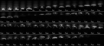


 Open access