


1. Introduction
Pulsar wind nebulae (PWNe) represent the majority of the identified TeV gamma-ray sources in the Galactic plane (Abdalla et al. Reference Abdalla2018a,b). The TeV emission is generally believed to be of leptonic origin, where high energy electrons are accelerated after crossing the pulsar termination shock, and scatter soft photons to produce inverse-Compton (IC) radiation at TeV gamma-ray energies. The interstellar medium (ISM) greatly affects the morphology of the PWN observed from radio up to gamma-ray energies. For instance, the interaction between the progenitor SNR and a nearby molecular cloud (MC) leads to an offset position of the pulsar with respect to the TeV peak along the pulsar-MC axis (Blondin, Chevalier, & Frierson Reference Blondin, Chevalier and Frierson2001).
In this paper, we investigate the ISM towards seven TeV PWNe and PWN candidates (Acero et al. Reference Acero2013; Abdalla et al. Reference Abdalla2018a). We make use of the Nanten CO(1–0) survey (Mizuno & Fukui Reference Mizuno, Fukui, Clemens, Shah and Brainerd2004) to illustrate the wide-field morphology of the diffuse molecular gas towards the PWNe and 7-mm Mopra spectral line observations to probe the dense molecular, and possibly shocked, gas along with star-forming regions. An accurate description of the ISM can help explain the morphology of the PWN (e.g. Vela X, Moriguchi et al. Reference Moriguchi, Yamaguchi, Onishi, Mizuno and Fukui2001; Slane et al. Reference Slane2018). Linking each TeV source to its local ISM can also provide additional constraints on its distance. We can identify target material for hadronic components (i.e. cosmic rays, CRs) escaping the TeV source, for example, from a progenitor supernova remnant (e.g. Voisin et al. Reference Voisin, Rowell, Burton, Walsh, Fukui and Aharonian2016). Lastly, by combining ISM mapping with the improved sensitivity and angular resolution of the next-generation Cerenkov Telescope Array (CTA, Acharya et al. Reference Acharya2013, Reference Acharya2017), we will be able to study the diffusion process of high energy particles towards and inside the ISM clouds.
This paper is organised as follows. In Section 2, we briefly outline the technical properties of the Mopra and Nanten telescopes as well as the analysis used for our 7-mm Mopra data reduction. We provide the results towards the different individual sources in Section 3 and discuss the nature of the TeV source in Section 4.
2. ISM data and analysis procedure
2.1. 7-mm Mopra data and analysis
We conducted 20′ × 20′ and 10′ × 10′ observations of the ISM towards several HESS TeV sources as part of our ‘MopraGam’ survey.Footnote a The 7-mm observations towards these studied sources were carried out between 2012 and 2015. Table 1 indicates the position and size of the different observations towards the seven regions that were mapped.
Table 1. Mopra 7-mm coverage of the TeV sources studied in this paper. The central position in (RA, Dec) and size is given for all observations undertaken towards the TeV sources.
We used the Mopra spectrometer MOPS in ‘zoom’ mode, which records 16 sub-bands, each consisting of 4 096 channels over a 137.5-MHz bandwidth. The ‘on the fly mapping’ (OTF) Nyquist sampled these regions with a 1′ beam size and a velocity resolution of ∼ 0.2 km/s. We can thus simultaneously observe tracers that can help understand the structure and morphology of MCs. Among the tracers observed in this paper, both the carbon monosulfide and cyanoacetylene transitions CS(1–0) and HC3N(5 − 4, F = 4 − 3) can be found in dense molecular gas and star-forming regions (Irvine, Goldsmith, & Hjalmarson Reference Irvine, Goldsmith, Hjalmarson, Hollenbach and Thronson1987). Silicon monoxide SiO emission can also be detected inside shocked dense MCs (Schilke et al. Reference Schilke, Walmsley, Pineau des Forets and Flower1997; Gusdorf et al. Reference Gusdorf, Cabrit, Flower and Pineau Des Forêts2008) and is a good signpost to claim physical association between an SNR and a nearby MC (e.g. see Nicholas et al. Reference Nicholas, Rowell, Burton, Walsh, Fukui, Kawamura and Maxted2012). Finally, the 44-GHz methanol class I maser CH3OH(I) generally indicates nearby active star-forming regions (Voronkov et al. Reference Voronkov, Caswell, Ellingsen, Green and Breen2014).
2.1.1. Data reduction
We used LivedataFootnote
b
to produce the spectra of each observation, calibrated by an OFF position, and subtracted the baseline using a linear fit. Then, we used Gridzilla
Footnote
c
to obtain a 3D cube showing the variation of the antenna temperature $T_{\textrm{A}}^{*}$
as a function of position and line of sight velocity v
lsr. Each region was mapped with a pixel spacing of 15″. After a careful look at the data, we recursively performed linear and sinusoidal fits on each pixel in order to remove baseline ripples. Notably, each sinusoidal fit was performed with different initial wavelengths to account for ripples of various sizes. Velocity ranges with significant emission were masked during these fits. The cleaned data cubes were then smoothed via a Gaussian with a full width at half maximum (FWHM) of 1.25′ so as to mitigate spatial fluctuations. Finally, the cubes were Hanning smoothed using five channels in order to remove spikes, reduce the T
rms, and highlight broader CS(1–0) emission. An overview of the reduction can be found in Appendix A.
$T_{\textrm{A}}^{*}$
as a function of position and line of sight velocity v
lsr. Each region was mapped with a pixel spacing of 15″. After a careful look at the data, we recursively performed linear and sinusoidal fits on each pixel in order to remove baseline ripples. Notably, each sinusoidal fit was performed with different initial wavelengths to account for ripples of various sizes. Velocity ranges with significant emission were masked during these fits. The cleaned data cubes were then smoothed via a Gaussian with a full width at half maximum (FWHM) of 1.25′ so as to mitigate spatial fluctuations. Finally, the cubes were Hanning smoothed using five channels in order to remove spikes, reduce the T
rms, and highlight broader CS(1–0) emission. An overview of the reduction can be found in Appendix A.
2.1.2. Producing CS(1–0) integrated intensity maps
We used the 7-mm CS(1–0) transition to probe the denser gas. The standard method to produce CS(1–0) integrated intensity maps is to sum the temperature $T_\textrm{A}^{*}$
of each channel within a given velocity range. However, in the case where detections span a large velocity range (Δv
lsr ∼ 10 to 30 km/s), any narrow CS(1–0) detections are likely to fall below the noise level, as a large portion of the noise may be included. In order to deal with this issue, we adopted the method described in Appendix A. This method, although more complex, provides a lower T
rms and cleaner integrated intensity maps, which could be used for multi-wavelength studies towards TeV sources.
$T_\textrm{A}^{*}$
of each channel within a given velocity range. However, in the case where detections span a large velocity range (Δv
lsr ∼ 10 to 30 km/s), any narrow CS(1–0) detections are likely to fall below the noise level, as a large portion of the noise may be included. In order to deal with this issue, we adopted the method described in Appendix A. This method, although more complex, provides a lower T
rms and cleaner integrated intensity maps, which could be used for multi-wavelength studies towards TeV sources.
2.1.3. Physical properties of CS(1–0) regions
From the CS(1–0) integrated intensity maps, we have selected clumps whose angular diameters were equal or greater than our Mopra CS beam size θ FWHM ∼ 1.6′. At the component velocity range, we fitted the CS(1–0) emission with Gaussian distributions.
We then used the Galactic rotation curve model from Brand & Blitz (Reference Brand and Blitz1993) to obtain near/far kinematic distance estimates based on the peak velocity of each detection. In the case where the isotopologue C34S(1–0) is detected, we use Eq. D.1 to derive the averaged optical depth τ
CS(1–0), using the isotopologue ratio α = 32S/34S ∼ 24, based on terrestrial measurements (Fink Reference Fink1981). Otherwise, an optically thin scenario τ
CS(1–0) = 0 was adopted. We obtained the column density of the upper state $N_{\textrm{CS}_1}$
using Eq. D.2. Assuming the gas to be in local thermal equilibrium, we thus obtained the total CS column density N
CS using Eq. D.3, assuming a kinetic temperature T
kin = 10 K typical of cold dense MCs. The CS to H2 abundance ratio X
CS inside dense molecular clumps varies between 10−9 and 10−8 as suggested by Irvine et al. (Reference Irvine, Goldsmith, Hjalmarson, Hollenbach and Thronson1987). In this work, we chose X
CS = 4 × 10⁻⁹ as per Zinchenko et al. (Reference Zinchenko, Forsstroem, Lapinov and Mattila1994) who studied MCs associated with star-forming regions. As a result, we expect our H2 column density estimates to systematically vary by a factor of 2. Finally, we use Eqs. D.4 and D.5 to determine the total mass
$N_{\textrm{CS}_1}$
using Eq. D.2. Assuming the gas to be in local thermal equilibrium, we thus obtained the total CS column density N
CS using Eq. D.3, assuming a kinetic temperature T
kin = 10 K typical of cold dense MCs. The CS to H2 abundance ratio X
CS inside dense molecular clumps varies between 10−9 and 10−8 as suggested by Irvine et al. (Reference Irvine, Goldsmith, Hjalmarson, Hollenbach and Thronson1987). In this work, we chose X
CS = 4 × 10⁻⁹ as per Zinchenko et al. (Reference Zinchenko, Forsstroem, Lapinov and Mattila1994) who studied MCs associated with star-forming regions. As a result, we expect our H2 column density estimates to systematically vary by a factor of 2. Finally, we use Eqs. D.4 and D.5 to determine the total mass $M_{\textrm{H}_2}\left(\textrm{CS}\right)$
and H2 density
$M_{\textrm{H}_2}\left(\textrm{CS}\right)$
and H2 density $n_{\textrm{H}_2}\left(\textrm{CS}\right)$
. The Gaussian fits for the CS(1–0) components towards the regions of the individual TeV sources can be found in Tables C.1–C.6 and their derived physical properties in Tables D.1–D.6.
$n_{\textrm{H}_2}\left(\textrm{CS}\right)$
. The Gaussian fits for the CS(1–0) components towards the regions of the individual TeV sources can be found in Tables C.1–C.6 and their derived physical properties in Tables D.1–D.6.
2.2. CO(1–0) data and analysis
While the Mopra CO(1–0) survey is well under way (see Braiding et al. Reference Braiding2015, Reference Braiding2018), we used for this work the 4-m Nanten CO(1–0) survey (Mizuno & Fukui Reference Mizuno, Fukui, Clemens, Shah and Brainerd2004), as it encompassed all our sources. The Nanten telescope CO(1–0) survey covered the Galactic plane with a 4′ sampling grid, a velocity resolution Δv = 0.625 km/s, and an averaged noise temperature per channel of ∼ 0.4 K.
The CO(1–0) emission probes the more diffuse molecular gas surrounding PWNe. As PWNe expand inside a low-density medium, we seek velocity ranges where the CO(1–0) emission spatially anti-corresponds with the TeV emission as that would support the PWN scenario (see Section 4.2). Molecular gas may also provide sufficient target material to produce hadronic TeV emission. Therefore, probing extended CO(1–0) emission overlapping the TeV emission is also a powerful means to test the hadronic scenario in the vicinity of a CR accelerator.
We arbitrarily selected CO regions based on the prominence of the CO(1–0) integrated emission compared to the rest of the maps and their proximity with the TeV gamma-ray source, as these can be helpful to test the hadronic/leptonic scenario (see Section 4). In the case where the pulsar is offset from the observed TeV gamma-ray source (i.e. HESS J1026–583), we highlight molecular regions which could produce such asymmetry along the pulsar-MC axis. We also derive physical parameters towards some extended regions defined from our CS detections (e.g. see HESS J1809–193 and HESS J1418–609). Assuming that all the gas traced by CO is embedded within this CS region, we are able to derive an upper limit on the averaged density $n_{\textrm{H}_2}$
.
$n_{\textrm{H}_2}$
.
We fitted the CO components at the velocity range of interest, with Gaussian distributions. We then used the X-factor X
CO = 2 × 1020 cm−2/(K km/s) to convert the CO integrated intensity into H2 column density. Bolatto, Wolfire, and Leroy (Reference Bolatto, Wolfire and Leroy2013) have argued that this value is correct to ∼ 30% across the Galactic plane. We then used Eq. D.4 to obtain the total molecular mass $M_{\textrm{H}_2}\left(\textrm{CO}\right)$
of the cloud, accounting for a 20% contribution from helium. We finally assumed a prolate geometry to obtain the H2 volume occupied by the molecular gas, and the averaged particle density
$M_{\textrm{H}_2}\left(\textrm{CO}\right)$
of the cloud, accounting for a 20% contribution from helium. We finally assumed a prolate geometry to obtain the H2 volume occupied by the molecular gas, and the averaged particle density $n_{\textrm{H}_2}\left(\textrm{CO}\right)$
using Eq. D.5 (see Appendix D). The Gaussian fits for the CO(1–0) components towards the regions of the individual TeV source can be found in Tables C.1–C.6 and their derived physical properties in Tables D.1–D.6.
$n_{\textrm{H}_2}\left(\textrm{CO}\right)$
using Eq. D.5 (see Appendix D). The Gaussian fits for the CO(1–0) components towards the regions of the individual TeV source can be found in Tables C.1–C.6 and their derived physical properties in Tables D.1–D.6.
2.3. HI analysis with SGPS/GASS surveys
From the Southern Galactic Plane Survey (SGPS) and GASS Hi surveys (McClure-Griffiths et al. Reference McClure-Griffiths, Dickey, Gaensler, Green, Haverkorn and Strasser2005; McClure-Griffiths et al. Reference McClure-Griffiths2009), we also obtained the atomic Hi column density N
Hi
assuming the (optically thin) conversion factor X
Hi
= 1.8 × 1018 cm−2/(K km/s) (Dickey & Lockman Reference Dickey and Lockman1990). Hi self-absorption may however occur towards colder Hi regions and, as a result, the optically thin assumption may underestimate N
Hi
by a factor of 2 (Fukui et al. Reference Fukui, Torii, Onishi, Yamamoto, Okamoto, Hayakawa, Tachihara and Sano2015). Comparing the total column density $N_{\textrm{H}}\,{=}\,N_{\textrm{H}\textsc{i}}+2N_{\textrm{H}_2}$
to the absorbed X-ray column density from X-ray counterparts can provide further constraints on the distance to the TeV source. The images showcasing the evolution of the total column density as a function of v
lsr and distance towards several TeV sources can be found in Appendix E. Atomic gas should also be accounted for while testing the hadronic scenario towards TeV sources. Consequently, as per the CO(1–0) emission, we derived the atomic masses
$N_{\textrm{H}}\,{=}\,N_{\textrm{H}\textsc{i}}+2N_{\textrm{H}_2}$
to the absorbed X-ray column density from X-ray counterparts can provide further constraints on the distance to the TeV source. The images showcasing the evolution of the total column density as a function of v
lsr and distance towards several TeV sources can be found in Appendix E. Atomic gas should also be accounted for while testing the hadronic scenario towards TeV sources. Consequently, as per the CO(1–0) emission, we derived the atomic masses $M_{\textrm{H}_I}$
towards the selected CO regions. These masses can be found in Tables D.1–D.6.
$M_{\textrm{H}_I}$
towards the selected CO regions. These masses can be found in Tables D.1–D.6.
3. The ISM found towards the TeV sources
We list here various detections from our 7-mm observations. For each source (see Figures 1–11) we labelled the regions with CS(1–0) detections in numerical order (e.g. ‘1’) while the regions with SiO(1–0, v = 0), HC3N(5–4, F = 4–3), CH3OH(I) detections are labelled ‘S’, ‘HC’, and ‘CH’, respectively. In this section however, we focus on combining our CS(1–0) detections with the Nanten CO(1–0) and primarily focus on the morphology of the various molecular regions surrounding our TeV PWNe and PWN candidates, which is useful to understand their nature and morphology.
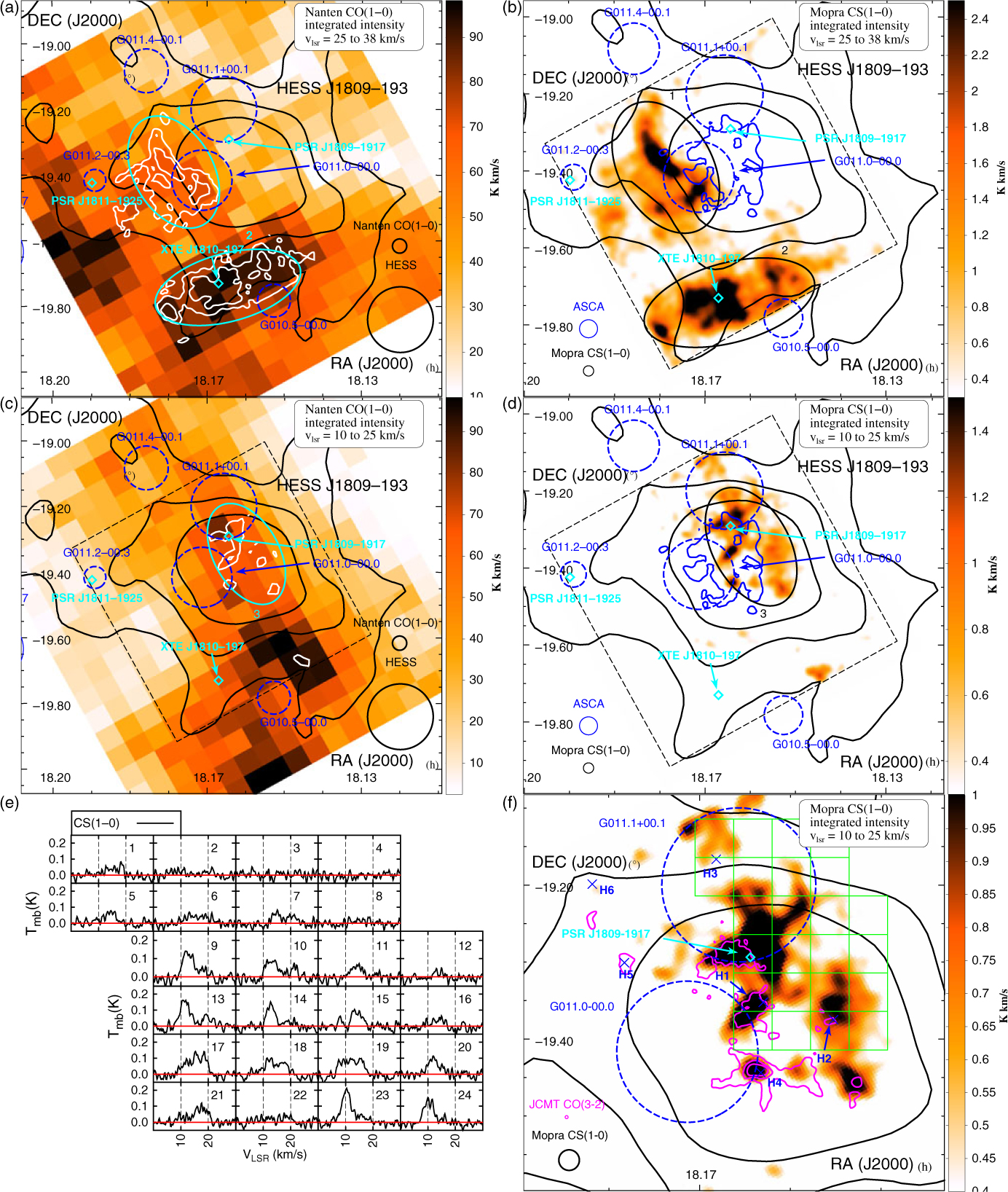
Figure 1. Nanten CO(1–0) and Mopra CS(1–0) integrated intensity maps across two velocity bands v lsr = 25 to 38 km/s (panels a and b) and v lsr = 10 to 25 km/s (panels c and d) towards HESS J1809–193 overlaid by the TeV gamma-ray counts in black contours (Aharonian et al. Reference Aharonian2007). The dashed black box represents the area covered during our 7-mm survey. The ellipses selected for CO and CS analyses (see Section 3.1) are shown in cyan and black, respectively. The SNRs are shown as dashed blue circles while the detected pulsars are shown as cyan diamonds. The ASCA hard X-ray (2–10 keV) contours are displayed on the right panels in blue while the CS white contours overlays are shown on the left panels. A zoomed image of the CS(1–0) integrated intensity emission at v lsr = 10 − 25 km/s is shown in panel f overlaid by the JCMT CO(2–1) integrated intensity contours in magenta. The position of Hii regions ‘H1→H5’ are shown in blue crosses. The averaged CS(1–0) emission over the green grid of boxes in panel f is displayed in panel e (see colour version online).
3.1. HESS J1809-193
HESS J1809–193 is a bright and extended TeV source whose position is coincident with several potential CR accelerators (Aharonian et al. Reference Aharonian2007). HAWC has also recently detected the TeV source 2HWC J1809–190, associated with HESS J1809–193 (Abeysekara et al. Reference Abeysekara2017). Araya (Reference Araya2018) recently found extended GeV emission associated with HESS J1809–193.
ASCA (Bamba et al. Reference Bamba, Ueno, Koyama and Yamauchi2003) and Suzaku observations (Anada et al. Reference Anada, Bamba, Ebisawa and Dotani2010) revealed non-thermal X-rays likely associated with the pulsar PSR J1809–1917 (shown as a cyan diamond in Figure 1 and pink in Figure 2), with spin down power $\dot{E}_{\textrm{SD}}=1.8\times10^{36}\,{\rm {erg\,s^{-1}}}$
, a characteristic age τ
c = 51 kyr and a dispersion measure distance d ∼ 3.7 kpc (Cordes et al. Reference Cordes, Lazio, Chatterjee, Arzoumanian and Chernoff2002). The presence of two SNR shells G011.0–0.0 and G011.1+0.1 (shown as blue circles in Figure 1) both observed at 330 and 1 465 MHz (Brogan et al. Reference Brogan, Devine, Lazio, Kassim, Tam, Brisken, Dyer and Roberts2004; Castelletti, Giacani, & Petriella Reference Castelletti, Giacani and Petriella2016) adds more complexity to the picture. Additionally, the ∼2 kyr old millisecond pulsar PSR J1811–1925 with spin down energy
$\dot{E}_{\textrm{SD}}=1.8\times10^{36}\,{\rm {erg\,s^{-1}}}$
, a characteristic age τ
c = 51 kyr and a dispersion measure distance d ∼ 3.7 kpc (Cordes et al. Reference Cordes, Lazio, Chatterjee, Arzoumanian and Chernoff2002). The presence of two SNR shells G011.0–0.0 and G011.1+0.1 (shown as blue circles in Figure 1) both observed at 330 and 1 465 MHz (Brogan et al. Reference Brogan, Devine, Lazio, Kassim, Tam, Brisken, Dyer and Roberts2004; Castelletti, Giacani, & Petriella Reference Castelletti, Giacani and Petriella2016) adds more complexity to the picture. Additionally, the ∼2 kyr old millisecond pulsar PSR J1811–1925 with spin down energy $\dot{E}_{\textrm{SD}}=6.4\times 10^{36} \,{\rm {erg\,s^{-1}}}$
(Torii et al. Reference Torii, Tsunemi, Dotani, Mitsuda, Kawai, Kinugasa, Saito and Shibata1999) and its progenitor SNR G011.2–0.3, located at d ∼ 4.4 to 7 kpc, are also positioned adjacent to HESS J1809–193 (see Figures 1 and 2) and thus might also contribute to the TeV emission. Finally, the anomalous X-ray magnetar XTE J1810–197 with period P = 5.54 s and period derivative
$\dot{E}_{\textrm{SD}}=6.4\times 10^{36} \,{\rm {erg\,s^{-1}}}$
(Torii et al. Reference Torii, Tsunemi, Dotani, Mitsuda, Kawai, Kinugasa, Saito and Shibata1999) and its progenitor SNR G011.2–0.3, located at d ∼ 4.4 to 7 kpc, are also positioned adjacent to HESS J1809–193 (see Figures 1 and 2) and thus might also contribute to the TeV emission. Finally, the anomalous X-ray magnetar XTE J1810–197 with period P = 5.54 s and period derivative $\dot{P}=1.8\times10^{-12}\,{\rm {s\,s^{-1}}}$
is located ∼ 0.35° south of HESS J1809–193.
$\dot{P}=1.8\times10^{-12}\,{\rm {s\,s^{-1}}}$
is located ∼ 0.35° south of HESS J1809–193.
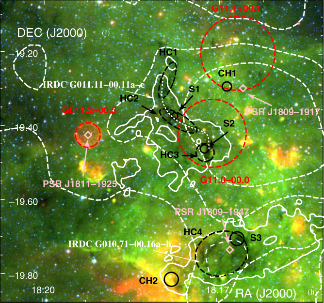
Figure 2. Three colours image showing the MIPSGAL 24 μm and GLIMPSE 8 μm and 4.6 μm in red, green, and blue, respectively, towards HESS J1809–193 overlaid by the HESS TeV gamma-ray counts in dashed white contours and CS(1–0) integrated intensity between v lsr = 25 to 38 km/s contours (0.6 K) in solid white. The SNRs are shown in red dashed circles, while the pulsars position are indicated in pink diamonds. The black dashed ellipses labelled ‘HC’ indicates the positions of HC3N(5–4,F = 4–3) detections, while the black solid circles labelled ‘CH’ and ‘S’, respectively, indicate CH3OH and SiO(1–0,v = 0) detections. The spectra of these regions can be found in Figure 3. The white dotted lines represent the extent of the infrared dark clouds IRDC G010.71–00.16a–h and IRDC G011.11–00.11a–e. (see colour version online)
Based on the kinematic distance of PSR J1809–1917 (d ∼ 3.7 kpc), we here focus on components at v lsr = 10 − 38 km/s (see blue and pink regions in Figure 3), although our Nanten CO(1–0) data have revealed several other components in the line of sight (see CO(1–0) emission in Figure 3).
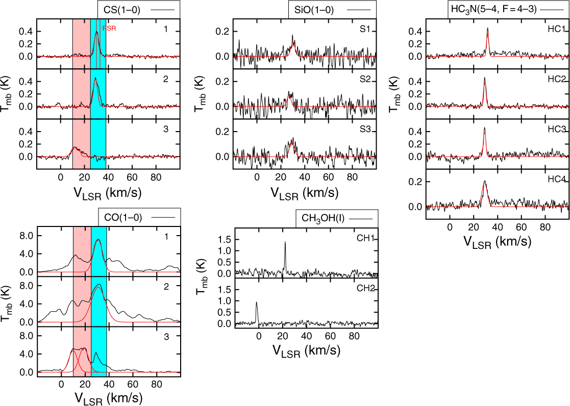
Figure 3. Averaged CS(1–0), CO(1–0), SiO(1–0, v = 0), CH3OH(I), and HC3N(5–4, F = 4–3) spectra towards the emission from the selected regions in Figures 1 and 2 towards HESS J1809–193. The solid red lines represent the Gaussian fit of the emission whose parameters are shown in Table C.1. The two red vertical lines indicate the pulsar PSR J1809–1917 dispersion measure distance converted to kinematic velocity. The pink and cyan regions represent the velocity range for the CS(1–0) and CO(1–0) integrated intensity maps displayed in Figure 1.
At this velocity range, we remark that the molecular gas generally overlaps the TeV emission shown in black contours. Notably, at v lsr = 25 to 38 km/s (d ∼ 3.7 kpc), prominent CO emission is found south and east of the TeV emission, while the prominent CO emission spatially overlaps the TeV emission at v lsr = 10 − 25 km/s (d ∼ 2.7 kpc). Our Mopra CS(1–0) integrated intensity maps (see Figure 1 panels b, d, and f) however provide a clear view of the dense gas.
At v
lsr = 25 to 38 km/s (Figure 1, panels a and b), the MCs in the regions labelled ‘1’ and ‘2’ and located east and south of SNR G011.0+00.0, respectively, appear very extended. From our CO and CS analyses, the masses derived in region ‘1’ attain $M_{\textrm{H}_2}\left(\textrm{CO}\right)=8.1\times10^{4}{\textrm{M}_{\odot}}$
and
$M_{\textrm{H}_2}\left(\textrm{CO}\right)=8.1\times10^{4}{\textrm{M}_{\odot}}$
and $M_{\textrm{H}_2}\left(\textrm{CS}\right)=3.2\times10^{4}{\textrm{M}_{\odot}}$
, while we obtain
$M_{\textrm{H}_2}\left(\textrm{CS}\right)=3.2\times10^{4}{\textrm{M}_{\odot}}$
, while we obtain $M_{\textrm{H}_2}\left(\textrm{CO}\right)=2.3\times10^{5}{\textrm{M}_{\odot}}$
and
$M_{\textrm{H}_2}\left(\textrm{CO}\right)=2.3\times10^{5}{\textrm{M}_{\odot}}$
and $M_{\textrm{H}_2}\left(\textrm{CS}\right)=3.2\times10^{4}{\textrm{M}_{\odot}}$
in region ‘2’. A significant fraction of the molecular gas in region ‘1’ and ‘2’ is therefore concentrated in clumps. The CS(1–0) emission in region ‘1’ also appears to anti-correspond with the ASCA X-ray diffuse emission shown in blue, supposedly produced by high energy electrons from the pulsar PSR J1809–1317 (see Anada et al. Reference Anada, Bamba, Ebisawa and Dotani2010).
$M_{\textrm{H}_2}\left(\textrm{CS}\right)=3.2\times10^{4}{\textrm{M}_{\odot}}$
in region ‘2’. A significant fraction of the molecular gas in region ‘1’ and ‘2’ is therefore concentrated in clumps. The CS(1–0) emission in region ‘1’ also appears to anti-correspond with the ASCA X-ray diffuse emission shown in blue, supposedly produced by high energy electrons from the pulsar PSR J1809–1317 (see Anada et al. Reference Anada, Bamba, Ebisawa and Dotani2010).
Interestingly, we have found embedded dense filaments in region ‘1’ from C34S(1–0) and HC3N(5–4, F = 4–3) detections (see Figure F.1 in Appendix F). In fact, the positions of the HC3N detections labelled ‘HC1 to HC3’ in Figure 2 coincide with the Spitzer infrared (IR) dark cloud IRDC G011.11–00.11a–e (Parsons, Thompson, & Chrysostomou Reference Parsons, Thompson and Chrysostomou2009, see dotted white lines in Figure 2), confirming the molecular gas is foreground to the IR emission.
We have also identified two weak but broad (FWHM ∼4 km/s) SiO(1–0) features in region ‘1’ (see Figures 2 and 3 for spectra), labelled ‘S1’ and ‘S2’. The absence of overlapping IR continuum emission indicates the lack of active star-forming regions and could indicate a possible interaction between the MC and a non-star-forming shock (Schilke et al. Reference Schilke, Walmsley, Pineau des Forets and Flower1997; Gusdorf et al. Reference Gusdorf, Cabrit, Flower and Pineau Des Forêts2008), which could here come from the adjacent SNR G011.0–0.0.
Based on the potential interaction between the SNR G011.0–0.0 and the dense MC at v
lsr ∼ 30 km/s, we thus suggest an alternate SNR distance d ∼ 3.7 kpc compared to the distance d ∼ 3.0 kpc claimed by Castelletti et al. (Reference Castelletti, Giacani and Petriella2016). If SNR G011.0–0.0 indeed interacted with the MC at d ∼ 3.7 kpc, it would then be located at the pulsar PSR J1809–1917 distance and quite likely be its progenitor SNR. Using eq. 3.33a from Cioffi, McKee, and Bertschinger (Reference Cioffi, McKee and Bertschinger1988), we derive that the ambient density required to match the small projected radius rSNR
∼ 5 pc with the pulsar characteristic age τ
c = 51 kyr is n
amb ∼ 370 cm−3. The averaged density $n_{\textrm{H}_2}\left(\textrm{CO}\right)=440\,{\rm{cm}}^{-3}$
found towards region ‘1’ appears somewhat consistent with this estimated averaged density.
$n_{\textrm{H}_2}\left(\textrm{CO}\right)=440\,{\rm{cm}}^{-3}$
found towards region ‘1’ appears somewhat consistent with this estimated averaged density.
In region ‘2’, we have also detected extended HC3N(5–4, F = 4–3) emission and C34S(1–0) emission overlapping the IR dark cloud IRDC G010.71–00.16a–h (Parsons et al. Reference Parsons, Thompson and Chrysostomou2009), highlighting another dense region. The morphology of the IR dark cloud and our HC3N detection appear elliptic and embed the anomalous X-ray magnetar XTE J1810–197 (see Gotthelf et al. Reference Gotthelf, Halpern, Buxton and Bailyn2004 and references therein), suggesting their potential physical association. Additionally, a prominent SiO(1–0) detection (see region ‘S3’ in Figure 2) was also found inside this dark cloud. This MC may thus be disrupted by another shock, perhaps caused by the progenitor SNR of XTE J1810–197.
At v lsr = 10 − 25 km/s (Figure 1 panel d), we observe several CS(1–0) components inside the region here labelled ‘3’. We notably find that the CS(1–0) prominent emission corresponds with the JCMT CO(3–2) peaks found by Castelletti et al. (Reference Castelletti, Giacani and Petriella2016) and the Hii regions (purple contours and blue crosses in Figure 1 panel f, respectively).
We observe that the CS(1–0) emission averaged over the grid regions (Figure 1 panels e–f) exhibits considerable variation of the peak velocity ranging between v lsr = 10 − 22 km/s. For example, the two peaks at v lsr ∼ 12 and 18 km/s inside ‘boxes 9 and 10’ merge to a single peaked emission with v lsr ∼ 15 km/s in ‘box 15’. This dense molecular region appears to host several Hii regions (see ‘H1–H3’ in Figure 1f). Consequently, the two spectral components may actually probe the same molecular gas, disrupted by the driving motion forces from various Hii regions. We also note that the MC anti-corresponds with the two SNRs. The disrupted gas could consequently be caused by one of these SNRs. As a result, we cannot rule out the SNR G011.0–0.0 distance d ∼3.0 kpc suggested by Castelletti et al. (Reference Castelletti, Giacani and Petriella2016).
3.2. HESS J1026–583
The TeV source HESS J1026–583 was discovered from energy dependent morphology studies towards HESS J1023–591 (Abramowski et al. Reference Abramowski2011). The latter source is thought to be powered by the colliding winds from Wolf–Rayet stars within the massive stellar cluster Westerlund 2 at $d=5.4^{+1.1}_{-1.4}$
kpc (Furukawa et al. Reference Furukawa, Dawson, Ohama, Kawamura, Mizuno, Onishi and Fukui2009). Acero et al. (Reference Acero2013) catalogued HESS J1026–583 as a PWN candidate based on the detection of a nearby radio quiet gamma-ray pulsar PSR J1028–5810 (Ray et al. Reference Ray2011) responsible for the GeV emission towards 3FGL J1028.4–5819 (shown as a red circle in Figure 4). PSR J1028–5819 has a spin down power
$d=5.4^{+1.1}_{-1.4}$
kpc (Furukawa et al. Reference Furukawa, Dawson, Ohama, Kawamura, Mizuno, Onishi and Fukui2009). Acero et al. (Reference Acero2013) catalogued HESS J1026–583 as a PWN candidate based on the detection of a nearby radio quiet gamma-ray pulsar PSR J1028–5810 (Ray et al. Reference Ray2011) responsible for the GeV emission towards 3FGL J1028.4–5819 (shown as a red circle in Figure 4). PSR J1028–5819 has a spin down power $\dot{E}_{\textrm{SD}}=8.3\times10^{35}\,{\rm {erg\,s^{-1}}}$
, characteristic age τ = 89 kyr, and a dispersion measure distance d = 2.3 ± 0.7 kpc. However, HESS J1026–583 shows a hard VHE spectral index Γ
γ
= 1.94. It also does not exhibit any X-rays that are spatially coincident with the TeV source. Additionally, diffuse GeV gamma-ray emission has been detected with Fermi-LAT towards Westerlund 2 (Yang, de Oña Wilhelmi, & Aharonian Reference Yang, de Oña Wilhelmi and Aharonian2017). The authors have argued for a hadronic origin based on its 200 pc extension of the 1–250 GeV emission. Consequently, a clear identification remains to be seen. Because of its proximity to HESS J1023–575, several ISM features have already extensively been studied (Dame Reference Dame2007; Fukui et al. Reference Fukui2009; Furukawa et al. Reference Furukawa, Dawson, Ohama, Kawamura, Mizuno, Onishi and Fukui2009; Furukawa et al. Reference Furukawa2014; Hawkes et al. Reference Hawkes2014).
$\dot{E}_{\textrm{SD}}=8.3\times10^{35}\,{\rm {erg\,s^{-1}}}$
, characteristic age τ = 89 kyr, and a dispersion measure distance d = 2.3 ± 0.7 kpc. However, HESS J1026–583 shows a hard VHE spectral index Γ
γ
= 1.94. It also does not exhibit any X-rays that are spatially coincident with the TeV source. Additionally, diffuse GeV gamma-ray emission has been detected with Fermi-LAT towards Westerlund 2 (Yang, de Oña Wilhelmi, & Aharonian Reference Yang, de Oña Wilhelmi and Aharonian2017). The authors have argued for a hadronic origin based on its 200 pc extension of the 1–250 GeV emission. Consequently, a clear identification remains to be seen. Because of its proximity to HESS J1023–575, several ISM features have already extensively been studied (Dame Reference Dame2007; Fukui et al. Reference Fukui2009; Furukawa et al. Reference Furukawa, Dawson, Ohama, Kawamura, Mizuno, Onishi and Fukui2009; Furukawa et al. Reference Furukawa2014; Hawkes et al. Reference Hawkes2014).
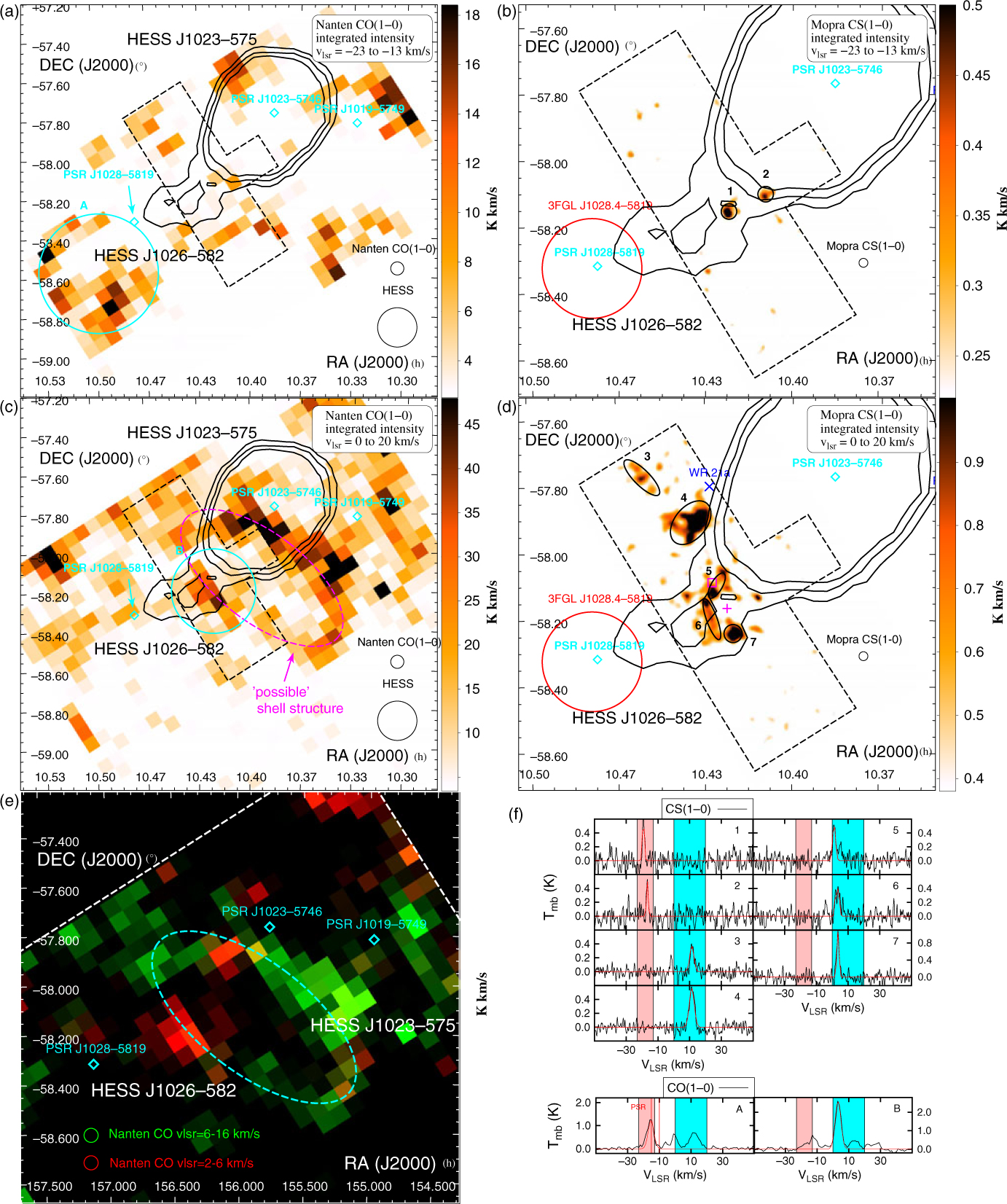
Figure 4. Nanten CO(1–0) and Mopra CS(1–0) emission between v lsr = −23 to 13 km/s and v lsr = 0 to 20 km/s towards HESS J1026–582 and HESS J1023–575 whose TeV gamma-ray counts are shown in black contours. The position of the pulsars PSR J1028–5819, PSR J1023–5746, and PSR J1019–5749 are indicated as cyan diamonds. The GeV emission 3FGL J1028–5819 is shown as a red circle. The cyan ellipses indicate the selected regions (labelled A and B) from our CO analysis, while the black circles (labelled 1 to 7 in panels b and d) show the position of selected CS(1–0) regions. The location of WR 21a is shown as a blue cross in panel d, while the purple square and cross indicate the position of the Hii region GAL 284.65–00.48 and the reflection nebula GN 10.23.6, respectively. Panel e is a two-colour image showing the Nanten CO(1–0) integrated intensity at v lsr = 2 to 6 km/s (red) and v lsr = 6 to 16 km/s (green) overlaid by the HESS TeV contours in white towards HESS J1026–582. The cyan dashed ellipse represents the possible molecular ring structure (see Section 3.2). Panel f illustrates the averaged CO(1–0) and CS(1–0) emission from the selected regions. The red lines indicate the fit used to model the emission (see Table C.2 for fit parameters). The two red vertical lines show the dispersion measure distance of the pulsar PSR J1018–5819. The blue and pink regions indicate the velocity range shown in panels a to d.
Figure 4 shows the Nanten CO(1–0) integrated intensity at v
lsr = −23 to −13 km/s (panel a) and 0 to 20 km/s (panel c), inferring a distance d ∼ 2.3 kpc and d ∼ 4.9 kpc, respectively, positioning the detections along the Carina arm (see Figure A.3 in Appendix B). At v
lsr = −23 to −13 km/s, we note that the CO emission does not overlap the TeV emission, nor the pulsar’s position. In fact, the molecular region with prominent CO emission, which we labelled ‘A’, is located east of the pulsar position, and could support the crushed PWN scenario (see Blondin et al. Reference Blondin, Chevalier and Frierson2001). Assuming a kinematic distance d ∼ 2.3 kpc, we obtain a total mass $M_{\textrm{H}_2}\left(\textrm{CO}\right)=9.7\times10^{3}{\textrm{M}_{\odot}}$
. Lastly, from our CS survey, we have also identified two unresolved CS(1–0) features labelled ‘1’ and ‘2’ in Figure 4 panel b.
$M_{\textrm{H}_2}\left(\textrm{CO}\right)=9.7\times10^{3}{\textrm{M}_{\odot}}$
. Lastly, from our CS survey, we have also identified two unresolved CS(1–0) features labelled ‘1’ and ‘2’ in Figure 4 panel b.
At v
lsr = 0 to 20 km/s (d ∼ 4.9 kpc, see Figure 4 panel c), we observe prominent CO emission at v
lsr ∼ 4 km/s, labelled ‘B’, spatially coincident with the HESS J1026–582 TeV peak. The MC in region ‘B’ with total mass $M_{\textrm{H}_2}\left(\textrm{CO}\right)=4.9\times10^{4}{\textrm{M}_{\odot}}$
appears next to a possible shell like structure (see dashed purple and cyan ellipses in Figure 4 panels c and e, respectively) which overlaps the HESS J1023–575 TeV emission. The molecular region is however located at the tangent of the Sagittarius arm (see Figure A.3); thus, it is possible that the various MCs found in Figure 4 panel c may be unrelated. From Figure 4 panel d, it nonetheless appears that the CO(1–0) emission at v
lsr = 2 to 6 km/s fills in some missing segment of the shell-like structure and might form a ring (indicated as a dashed-cyan ellipse) whose centre is located south-west of HESS J1026–582 observed at v
lsr = 6 to 16 km/s. The molecular structure at v
lsr = 6 to 16 km/s could therefore be physically connected to the MC in region ‘B’.
$M_{\textrm{H}_2}\left(\textrm{CO}\right)=4.9\times10^{4}{\textrm{M}_{\odot}}$
appears next to a possible shell like structure (see dashed purple and cyan ellipses in Figure 4 panels c and e, respectively) which overlaps the HESS J1023–575 TeV emission. The molecular region is however located at the tangent of the Sagittarius arm (see Figure A.3); thus, it is possible that the various MCs found in Figure 4 panel c may be unrelated. From Figure 4 panel d, it nonetheless appears that the CO(1–0) emission at v
lsr = 2 to 6 km/s fills in some missing segment of the shell-like structure and might form a ring (indicated as a dashed-cyan ellipse) whose centre is located south-west of HESS J1026–582 observed at v
lsr = 6 to 16 km/s. The molecular structure at v
lsr = 6 to 16 km/s could therefore be physically connected to the MC in region ‘B’.
Among the CS(1–0) features found at v
lsr = 0 to 20 km/s, the gas clumps labelled ‘5’ to ‘7’, embedded in the molecular gas in region ‘B’ form a partial shell structure overlapping the TeV peak emission with a combined mass $M_{\textrm{H}_2}\left(\textrm{CO}\right)\sim5.0\times10^{3}{\textrm{M}_{\odot}}$
, very similar to the CO mass obtained in region ‘B’. No massive stars have been catalogued towards the centre of this structure. However, we note the presence of the Hii region GAL 284.65–00.48 towards region ‘5’ and the reflective nebula GV 10.23.6 at the centre of the shell (see purple box and cross in Figure 4 panel d, respectively).
$M_{\textrm{H}_2}\left(\textrm{CO}\right)\sim5.0\times10^{3}{\textrm{M}_{\odot}}$
, very similar to the CO mass obtained in region ‘B’. No massive stars have been catalogued towards the centre of this structure. However, we note the presence of the Hii region GAL 284.65–00.48 towards region ‘5’ and the reflective nebula GV 10.23.6 at the centre of the shell (see purple box and cross in Figure 4 panel d, respectively).
3.3. HESS J1119–614
Djannati-Ataï (Reference Djannati-Ataï, Marandon and Chaves2009) and Abdalla et al. (Reference Abdalla2018a) reported the detection of the TeV source HESS J1119–614 (see solid black contours in Figure 5). It is thought to be associated with either the PWN, powered by the radio pulsar PSR J1119–6127 (see cyan diamond in Figure 5), with spin down period P = 400 ms (Camilo et al. Reference Camilo, Kaspi, Lyne, Manchester, Bell, D’Amico, McKay and Crawford2000) and characteristic age τ c = 1.9 kyr (Weltevrede, Johnston, & Espinoza Reference Weltevrede, Johnston and Espinoza2011); or its progenitor SNR G292.2–0.5 (see dashed blue circle in Figure 5). The 3″ × 3″ PWN has been resolved in X-ray with Chandra (Gonzalez & Safi-Harb Reference Gonzalez and Safi-Harb2005; Safi-Harb & Kumar Reference Safi-Harb and Kumar2008). The shell of progenitor SNR has been observed both in the radio band with ATCA (Crawford et al. Reference Crawford, Gaensler, Kaspi, Manchester, Camilo, Lyne and Pivovaroff2001), and in X-ray with ASCA between 0.4 and 10 keV (Pivovaroff et al. Reference Pivovaroff, Kaspi, Camilo, Gaensler and Crawford2001). Follow-up studies with Chandra and XMM-Newton (Kumar et al. Reference Kumar, Safi-Harb and Gonzalez2012; Ng et al. Reference Ng, Kaspi, Ho, Weltevrede, Bogdanov, Shannon and Gonzalez2012) revealed additional information about the nature of the X-ray emission. Indeed, from the four regions studied by Kumar et al. (Reference Kumar, Safi-Harb and Gonzalez2012) (here labelled ‘X1’ to ‘X4’ in Figure 5), the three regions ‘X1’ to ‘X3’ shown as blue ellipses have a non-thermal component. However, the X-ray emission in region ‘X4’ shown as a blue-pink ellipse is prominent and is thought to be of thermal origin.
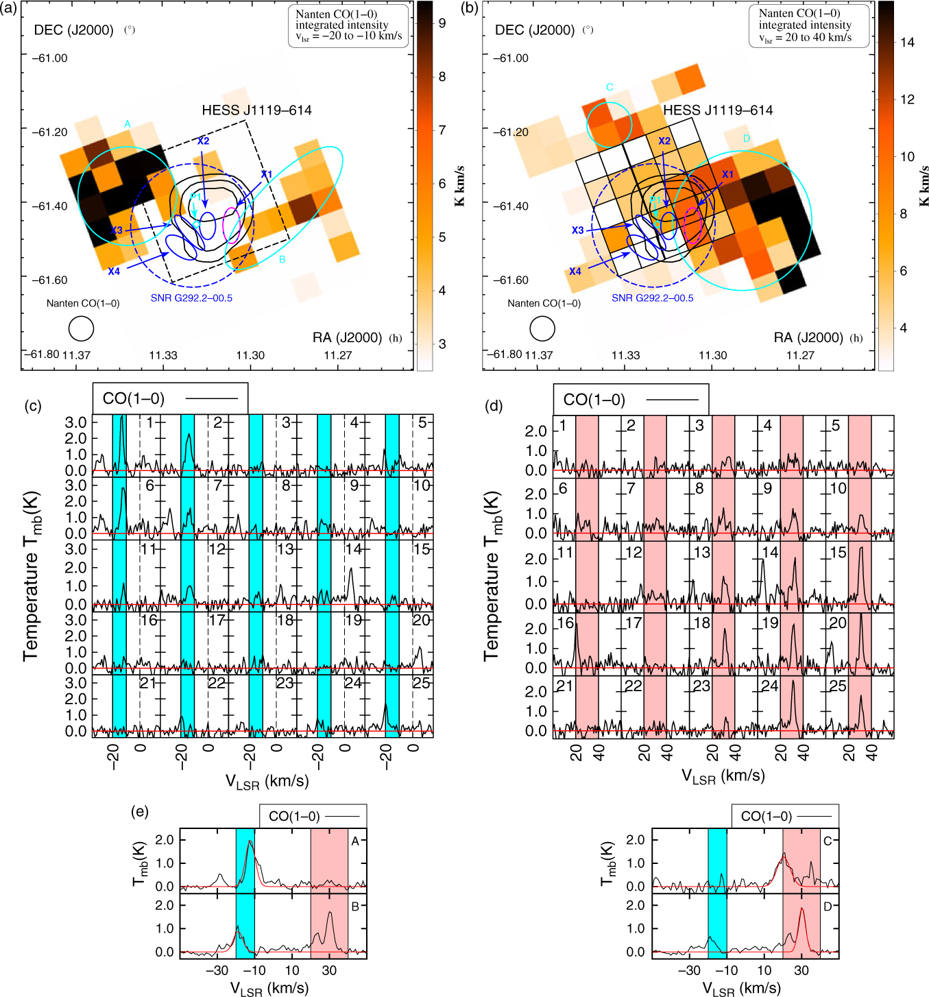
Figure 5. Nanten CO(1–0) emission between v lsr = −20 to −10 km/s (panel a) and v lsr = 20 to 40 km/s (panel b) towards HESS J1119–614 whose TeV gamma-ray emission is shown as solid black contours. The progenitor SNR G292.2–0.5 is delimited by the blue dashed circle. The solid blue and dashed blue-pink ellipses labelled ‘X1’ to ‘X4’ (see text) highlight bright X-ray regions studied by Kumar, Safi-Harb, & Gonzalez (Reference Kumar, Safi-Harb and Gonzalez2012) with XMM-Newton and Chandra. The pulsar PSR J1119–6127 (P1)’s position is indicated as a cyan diamond. The cyan ellipses show the selected regions (labelled A to D) for our CO analysis. Panels c and d show the variation of the averaged CO(1–0) spectra over the black grid of boxes shown in panel (b). The cyan and pink regions indicate the velocity ranges mapped in panels a and b. Panel e shows the averaged CO(1–0) emission from the selected regions towards HESS J1119–164. The red lines indicate the fit used to parametrise the emission. The fit parameters are displayed in Table C.5. The pink and cyan regions show the velocity range used for the above integrated intensity maps.
Caswell, McClure-Griffiths, & Cheung (Reference Caswell, McClure-Griffiths and Cheung2004) estimated a distance d ∼ 8.4 kpc for the pulsar and its progenitor SNR, based on the Hi and magnetic field studies. However, reconciling the characteristic age τ c = 1.9kyr of PSR J1119–6127 and the ∼ 25 pc diameter of the progenitor SNR requires a low-density medium (Ng et al. Reference Ng, Kaspi, Ho, Weltevrede, Bogdanov, Shannon and Gonzalez2012) and a massive progenitor star. Gonzalez & SafiHarb (Reference Gonzalez and Safi-Harb2005) argued for an SNR distance at d = 3.6 to 6.3 kpc by modelling the X-ray spectrum. Our gas study thus aims to provide additional constraints on the distance and how it could affect the nature of the TeV source.
No extended CS emission have been found towards this region. From our Nanten CO data, several components have been detected along the line of sight at v lsr ∼ −30 km/s, v lsr ∼ −10 km/s (near/far distance d ∼ 2.6/4.5 kpc, near Carina-arm, see Figure A.3), v lsr ∼ 20 km/s (distance d ∼ 8.6 kpc, far Carina-arm), v lsr ∼ 30 km/s (kinematic distance d ∼ 9.7 kpc, far Carina-arm).
At v
lsr = −20 to −10 km/s, we observe two MCs (labelled ‘A’ and ‘B’ in Figure 5 panel a) positioned north-east and west to the SNR, respectively, and with respective masses $M_{\textrm{H}_2}\left(\textrm{CO}\right)=2.3\times10^{4}{\textrm{M}_{\odot}}$
and
$M_{\textrm{H}_2}\left(\textrm{CO}\right)=2.3\times10^{4}{\textrm{M}_{\odot}}$
and $M_{\textrm{H}_2}\left(\textrm{CO}\right)=7.1\times10^{4}{\textrm{M}_{\odot}}$
. We also note that the molecular ISM anti-corresponds with all X-ray regions.
$M_{\textrm{H}_2}\left(\textrm{CO}\right)=7.1\times10^{4}{\textrm{M}_{\odot}}$
. We also note that the molecular ISM anti-corresponds with all X-ray regions.
At v
lsr ∼ 20 to 40 km/s we observe that the bulk of the molecular gas is found in two regions labelled ‘C’ and ‘D’, with masses $M_{\textrm{H}_2}\left(\textrm{CO}\right)=1.3\times10^{4}{\textrm{M}_{\odot}}$
and
$M_{\textrm{H}_2}\left(\textrm{CO}\right)=1.3\times10^{4}{\textrm{M}_{\odot}}$
and $M_{\textrm{H}_2}\left(\textrm{CO}\right)=2.3\times10^{5}{\textrm{M}_{\odot}}$
, respectively. The morphology of the gas overlaps the TeV gamma-ray detection. It also corresponds with the thermal X-ray in region ‘X1’ both at v
lsr ∼ 20 km/s and v
lsr ∼ 30 km/s (see Figure 5 panel d), highlighting potential SNR-MC interaction. The molecular gas also anti-corresponds with the other X-ray regions ‘X2’ to ‘X4’, thought to have non-thermal components likely produced by the high energy electrons from both the SNR and the PWN. Therefore, we argue that the morphology of the CO(1–0) both at v
lsr ∼ 20 km/s and v
lsr ∼ 30 km/s appears consistent with the X-ray results, inferring a source kinematic distance d = 8.6 − 9.7 kpc. We finally remark that these two components may be physically connected and highlight motion caused by the progenitor star.
$M_{\textrm{H}_2}\left(\textrm{CO}\right)=2.3\times10^{5}{\textrm{M}_{\odot}}$
, respectively. The morphology of the gas overlaps the TeV gamma-ray detection. It also corresponds with the thermal X-ray in region ‘X1’ both at v
lsr ∼ 20 km/s and v
lsr ∼ 30 km/s (see Figure 5 panel d), highlighting potential SNR-MC interaction. The molecular gas also anti-corresponds with the other X-ray regions ‘X2’ to ‘X4’, thought to have non-thermal components likely produced by the high energy electrons from both the SNR and the PWN. Therefore, we argue that the morphology of the CO(1–0) both at v
lsr ∼ 20 km/s and v
lsr ∼ 30 km/s appears consistent with the X-ray results, inferring a source kinematic distance d = 8.6 − 9.7 kpc. We finally remark that these two components may be physically connected and highlight motion caused by the progenitor star.
We also compare the column densities, shown in Figure E.1, towards the four X-ray regions. Towards the regions ‘X1’ and ‘X2’, we match the X-ray modelled column density N h (grey regions in Figure E.1 top panels) at v lsr = 22 − 30 km/s, also suggesting a distance d = 8.6 − 9.6 kpc, positioning the source in the far-Carina arm. Towards the X-ray regions ‘X3’ and ‘X4’ however, our column densities do not reach the X-ray one, or yield to unreasonable large distance d ∼ 15.5 kpc. Clumps unresolved by the Nanten CO(1–0) may account for the missing components. Our column density studies thus provide a lower-limit kinematic distance d > 8.6 kpc, consistent with our morphological studies and with Caswell et al. (Reference Caswell, McClure-Griffiths and Cheung2004). To explain both the large SNR radius and the enhanced thermal X-ray emission in region ‘X4’, we argue that the SNR once propagated in a low-density medium (Ng et al. Reference Ng, Kaspi, Ho, Weltevrede, Bogdanov, Shannon and Gonzalez2012), until it reached the denser gas in region ‘D’.
3.4. Kookaburra and rabbit
The two TeV sources HESS J1418–609 and HESS J1420–607 have been classified as PWNe based on their spatial coincidence with the X-ray (Roberts & Romani Reference Roberts and Romani1998) and GeV gamma-ray counterparts (Acero et al. Reference Acero2013). Ng, Roberts, & Romani (Reference Ng, Roberts and Romani2005) indicated that two diffuse non-thermal X-ray sources were associated with the pulsar PSR J1420–6048 (labelled P1 in Figure 6), a 68.2-ms period pulsar with spin down power $\dot{E}_{\textrm{SD}}=1.0\times10^{37}\,{\rm {erg\,s^{-1}}}$
, characteristic age τ
c = 13 kyr and dispersion measure distance d ∼ 5.6 kpc; and the 108-ms radio-quiet gamma-ray pulsar PSR J1418–6058 (labelled P2), with a characteristic age τ
c = 1.6 kyr. It has also been noted that P2’s location is offset (∼ 8.4′) from the HESS J1418 − 09 TeV peak.
$\dot{E}_{\textrm{SD}}=1.0\times10^{37}\,{\rm {erg\,s^{-1}}}$
, characteristic age τ
c = 13 kyr and dispersion measure distance d ∼ 5.6 kpc; and the 108-ms radio-quiet gamma-ray pulsar PSR J1418–6058 (labelled P2), with a characteristic age τ
c = 1.6 kyr. It has also been noted that P2’s location is offset (∼ 8.4′) from the HESS J1418 − 09 TeV peak.
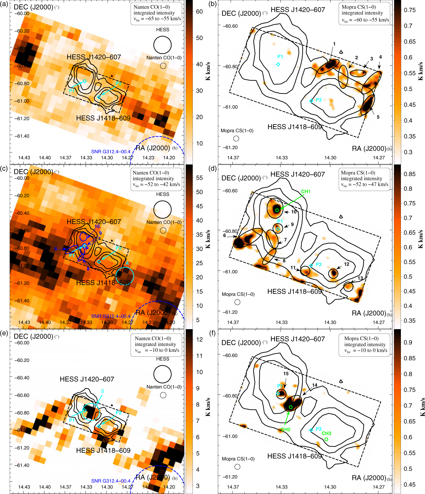
Figure 6. Nanten CO(1–0) and Mopra CS(1–0) emission between v lsr = −65 to −55 km/s, −52 to −42 km/s, and −10 to 0 km/s towards HESS J1420–607 and HESS J1418–609 shown in black contours. The black dashed box indicates our Mopra 7-mm coverage. The position of the pulsars PSR J1420–6048 and PSR J1418–6058 (labelled P1 and P2 here) are shown as cyan diamonds while the nearest SNR G312.4–0.04 is indicated as a blue dashed circle. Our CO regions ‘A’ and ‘B’ are shown in cyan in panels c and e. The blue ellipses on panel c and the black ellipses on the right panels indicate the position of the CS regions (‘1’ to ‘15’). The position of the CH3OH(I) detections labelled ‘CH1’ to ‘CH3’ are shown in green circles.
Roberts et al. (Reference Roberts, Brogan, Gaensler, Hessels, Ng and Romani2005) argue that the expected cometary shape of the PWN produced by a pulsar with a high space velocity would explain the offset position of the gamma-ray emission with respect to the pulsar. The distance to P2 has not yet been constrained. Ng et al. (Reference Ng, Roberts and Romani2005) have argued a PWN distance d = 2 to 5 kpc, while Wang (Reference Wang2011) has claimed a much smaller distance d = 1.4 − 1.9 kpc. Thus, by looking at the gas distribution in various velocity ranges, we aim to highlight the distance which would support the PWN scenario.
From our CO(1–0) observations, we have detected several molecular complexes along the line of sight. We mostly focus at the velocity ranges v lsr = −65 to −55 km/s, (d ∼ 5.6 kpc), ∼50 km/s (Scutum Crux arm, distance d ∼ 3.5 kpc), and ∼ −5 km/s (local arm, d ∼ 0.1 kpc), respectively, as shown in Figure 6. In Figure 7, we also note a CO component at v lsr ∼ −25 km/s. As opposed to the other velocity ranges, no prominent CS detections have been found at v lsr ∼ −25 km/s in this region, and thus we suggest that the MC is located on the far distance.
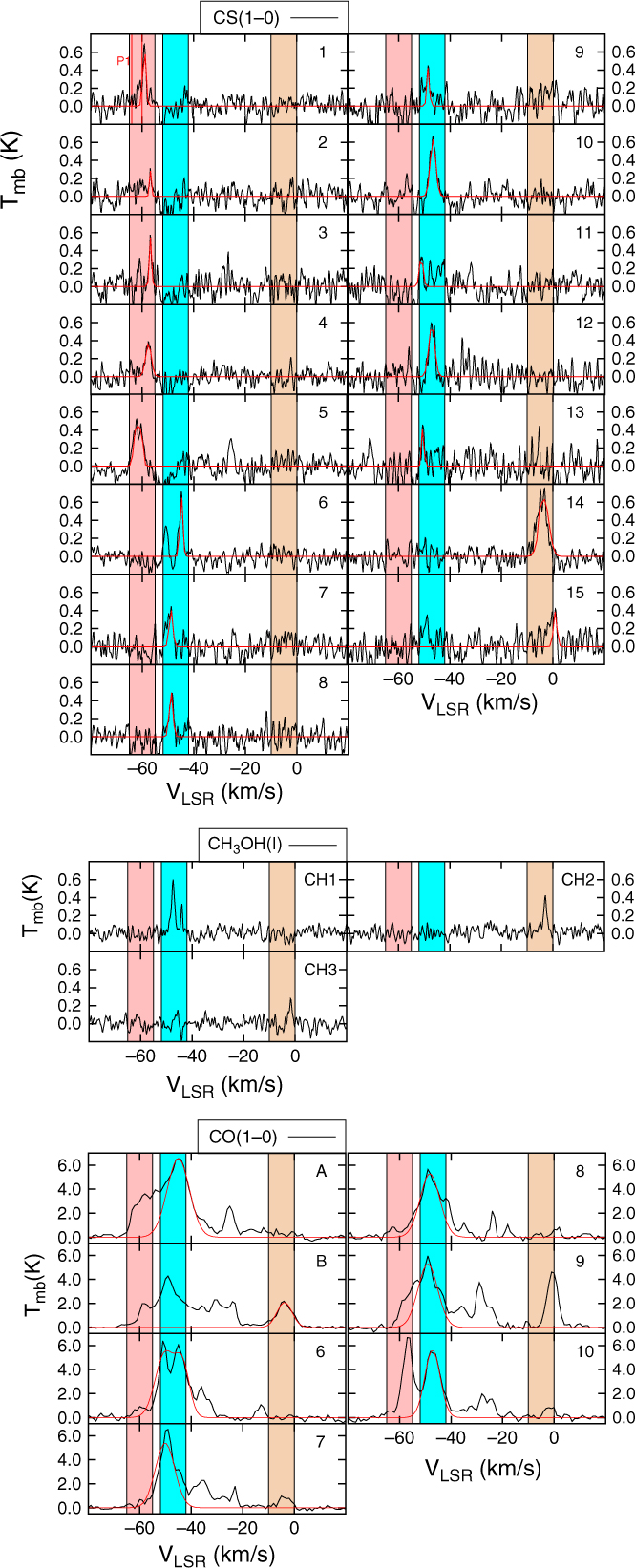
Figure 7. Averaged CS(1–0), CH3OH(I) and CO(1–0) emission from the regions towards HESS J1418–609 and HESS J1420–607 shown in Figure 6. The red lines indicate the fit used to model the emission at the velocity ranges where the regions are shown in Figure 6 (see Table C.4 for fit parameters). The red vertical lines show the dispersion measure distance of the pulsar PSR J1420–6048 (P1 in Figure 6). The pink, cyan and brown regions show the velocity ranges for the integrated intensity maps in Figure 6.
At v
lsr = −65 to −55 km/s (see Figure 6a), we note the bulk of the CO(1–0) emission is located towards the west and north side of HESS J1418–609. We also remark that the molecular emission shows little overlap with any of the TeV sources at this velocity range. We observed extended CS(1–0) emission, labelled ‘1’ to ‘5’, north of HESS J1418–609. Assuming a distance d = 5.6 kpc, the combined mass of these clumps attains $M_{\textrm{H}_2}\left(\textrm{CS}\right)=1.1\times10^{4}{\textrm{M}_{\odot}}$
. Notably, the bulk of the CS(1–0) emission appears to wrap around the TeV emission (as expected for leptonic IC emission).
$M_{\textrm{H}_2}\left(\textrm{CS}\right)=1.1\times10^{4}{\textrm{M}_{\odot}}$
. Notably, the bulk of the CS(1–0) emission appears to wrap around the TeV emission (as expected for leptonic IC emission).
At v
lsr = −52 to −42 km/s, we note that the CO(1–0) emission overlaps the two TeV sources, and peaks west of HESS J1018–609 and south east of HESS J1420–607. However, due to the small velocity separation between the components and the components at v
lsr = −65 to −55 km/s, it is somewhat difficult to accurately describe the morphology of the diffuse molecular gas at these velocities. We particularly observe that the prominent CO emission in region ‘A’, with mass $M_{\textrm{H}_2}\left(\textrm{CO}\right)=3.5\times10^{4}{\textrm{M}_{\odot}}$
and averaged density
$M_{\textrm{H}_2}\left(\textrm{CO}\right)=3.5\times10^{4}{\textrm{M}_{\odot}}$
and averaged density $n_{\textrm{H}_2}\left(\textrm{CO}\right)=5.6\times10^{2}\,{\rm {cm}}^{-3}$
, anti-corresponds with the TeV source HESS J1418–609. Our CS(1–0) results highlight a filamentary structure (see regions ‘6’ to ‘10’ in Figure 6d.), with a combined CS mass
$n_{\textrm{H}_2}\left(\textrm{CO}\right)=5.6\times10^{2}\,{\rm {cm}}^{-3}$
, anti-corresponds with the TeV source HESS J1418–609. Our CS(1–0) results highlight a filamentary structure (see regions ‘6’ to ‘10’ in Figure 6d.), with a combined CS mass $M_{\textrm{H}_2}\left(\textrm{CS}\right)=5.2\times10^{3}{\textrm{M}_{\odot}}$
(CO mass
$M_{\textrm{H}_2}\left(\textrm{CS}\right)=5.2\times10^{3}{\textrm{M}_{\odot}}$
(CO mass $M_{\textrm{H}_2}\left(\textrm{CO}\right)=3.1\times10^{4}{\textrm{M}_{\odot}}$
) which crosses HESS J1420–607. Interestingly, the dense gas in regions ‘6’ to ‘8’ also appears in a shell-like arrangement centred towards the south-east of HESS J1420–607. CS(1–0) clumps, labelled ‘11’ to ‘13’ are also found towards HESS J1418–609. The regions ‘11’ and ‘12’ are in fact coincident with the TeV peak emission.
$M_{\textrm{H}_2}\left(\textrm{CO}\right)=3.1\times10^{4}{\textrm{M}_{\odot}}$
) which crosses HESS J1420–607. Interestingly, the dense gas in regions ‘6’ to ‘8’ also appears in a shell-like arrangement centred towards the south-east of HESS J1420–607. CS(1–0) clumps, labelled ‘11’ to ‘13’ are also found towards HESS J1418–609. The regions ‘11’ and ‘12’ are in fact coincident with the TeV peak emission.
At v
lsr = −10 to 0 km/s (bottom panels), we found prominent CO emission south of HESS J1418–609, east of HESS J1420–607, and particularly between the two pulsars. Notably, the latter molecular region (labelled ‘B’) with mass $M_{\textrm{H}_2}\left(\textrm{CO}\right)=6.8{\textrm{M}_{\odot}}$
nests an extended dense clumps (see region ‘14’) with mass
$M_{\textrm{H}_2}\left(\textrm{CO}\right)=6.8{\textrm{M}_{\odot}}$
nests an extended dense clumps (see region ‘14’) with mass $M_{\textrm{H}_2}\left(\textrm{CS}\right)=2.7{\textrm{M}_{\odot}}$
and with averaged density reaching
$M_{\textrm{H}_2}\left(\textrm{CS}\right)=2.7{\textrm{M}_{\odot}}$
and with averaged density reaching $n_{\textrm{H}_2}\left(\textrm{CS}\right)=3.8\times10^{4}\,{\rm{cm}}^{-3}$
.
$n_{\textrm{H}_2}\left(\textrm{CS}\right)=3.8\times10^{4}\,{\rm{cm}}^{-3}$
.
In Figure E.2, we compare the column density from CO and Hi measurements with the column density $N_{\textrm{H}}=2.7\pm0.2\times10^{22}\,{\rm{cm}}^{-2}$
towards the pulsar PSR J1418–6058 derived from X-ray measurements (Kishishita et al. Reference Kishishita, Bamba, Uchiyama, Tanaka and Takahashi2012). Assuming that all components, except that at v
lsr ∼ 25 km/s, are in the near distance, we observe in Figure E.2 that the column density value from X-ray measurements is matched at v
lsr ≤ −50 km/s, which infers a distance range d ∼ 3.5 kpc. As a result, this column density X-ray study appears to favour a PWN location at d ∼ 3.5 kpc (v
lsr = −52 to −42 km/s), while our morphological study of the molecular ISM favours a PWN distance at d ∼5.6 kpc (v
lsr = −65 to −55 km/s), as it anti-corresponds with the TeV gamma-ray emission (see Figure 6).
$N_{\textrm{H}}=2.7\pm0.2\times10^{22}\,{\rm{cm}}^{-2}$
towards the pulsar PSR J1418–6058 derived from X-ray measurements (Kishishita et al. Reference Kishishita, Bamba, Uchiyama, Tanaka and Takahashi2012). Assuming that all components, except that at v
lsr ∼ 25 km/s, are in the near distance, we observe in Figure E.2 that the column density value from X-ray measurements is matched at v
lsr ≤ −50 km/s, which infers a distance range d ∼ 3.5 kpc. As a result, this column density X-ray study appears to favour a PWN location at d ∼ 3.5 kpc (v
lsr = −52 to −42 km/s), while our morphological study of the molecular ISM favours a PWN distance at d ∼5.6 kpc (v
lsr = −65 to −55 km/s), as it anti-corresponds with the TeV gamma-ray emission (see Figure 6).
3.5. HESS J1303-631
HESS J1303–631 was first classified as a ‘dark source’ due to its lack of any counterparts at other wavelengths (Aharonian et al. Reference Aharonian2005; Acero et al. Reference Acero2013). However, energy-dependent morphology of the TeV source (see Abramowski et al. Reference Abramowski2012b) unambiguously highlighted its association with the pulsar PSR J1301–6305 (P1 in Figure 8) with spin down energy $\dot{E}_{\textrm{SD}}=2.6\times10^{36}\,{\rm {erg\,s^{-1}}}$
, a rotation period P = 184 ms, and a characteristic age τ
c = 11 kyr. Follow-up observations with XMM-Newton revealed diffuse X-ray emission towards the pulsar with a power-law spectral index
$\dot{E}_{\textrm{SD}}=2.6\times10^{36}\,{\rm {erg\,s^{-1}}}$
, a rotation period P = 184 ms, and a characteristic age τ
c = 11 kyr. Follow-up observations with XMM-Newton revealed diffuse X-ray emission towards the pulsar with a power-law spectral index $\Gamma_X=2.0^{+0.6}_{-0.7}$
(Abramowski et al. Reference Abramowski2012b). Acero et al. (Reference Acero2013) detected a GeV counterpart with a gamma-ray spectral index Γ
γ
= 1.7. Finally, from the 1.384-GHz ATCA observations, Sushch et al. (Reference Sushch, Oya, Schwanke, Johnston and Dalton2017) recently announced the presence of a plausible SNR radio shell with radius ∼12′ next to the pulsar PSR J1301–6305, although this association appears unlikely.
$\Gamma_X=2.0^{+0.6}_{-0.7}$
(Abramowski et al. Reference Abramowski2012b). Acero et al. (Reference Acero2013) detected a GeV counterpart with a gamma-ray spectral index Γ
γ
= 1.7. Finally, from the 1.384-GHz ATCA observations, Sushch et al. (Reference Sushch, Oya, Schwanke, Johnston and Dalton2017) recently announced the presence of a plausible SNR radio shell with radius ∼12′ next to the pulsar PSR J1301–6305, although this association appears unlikely.
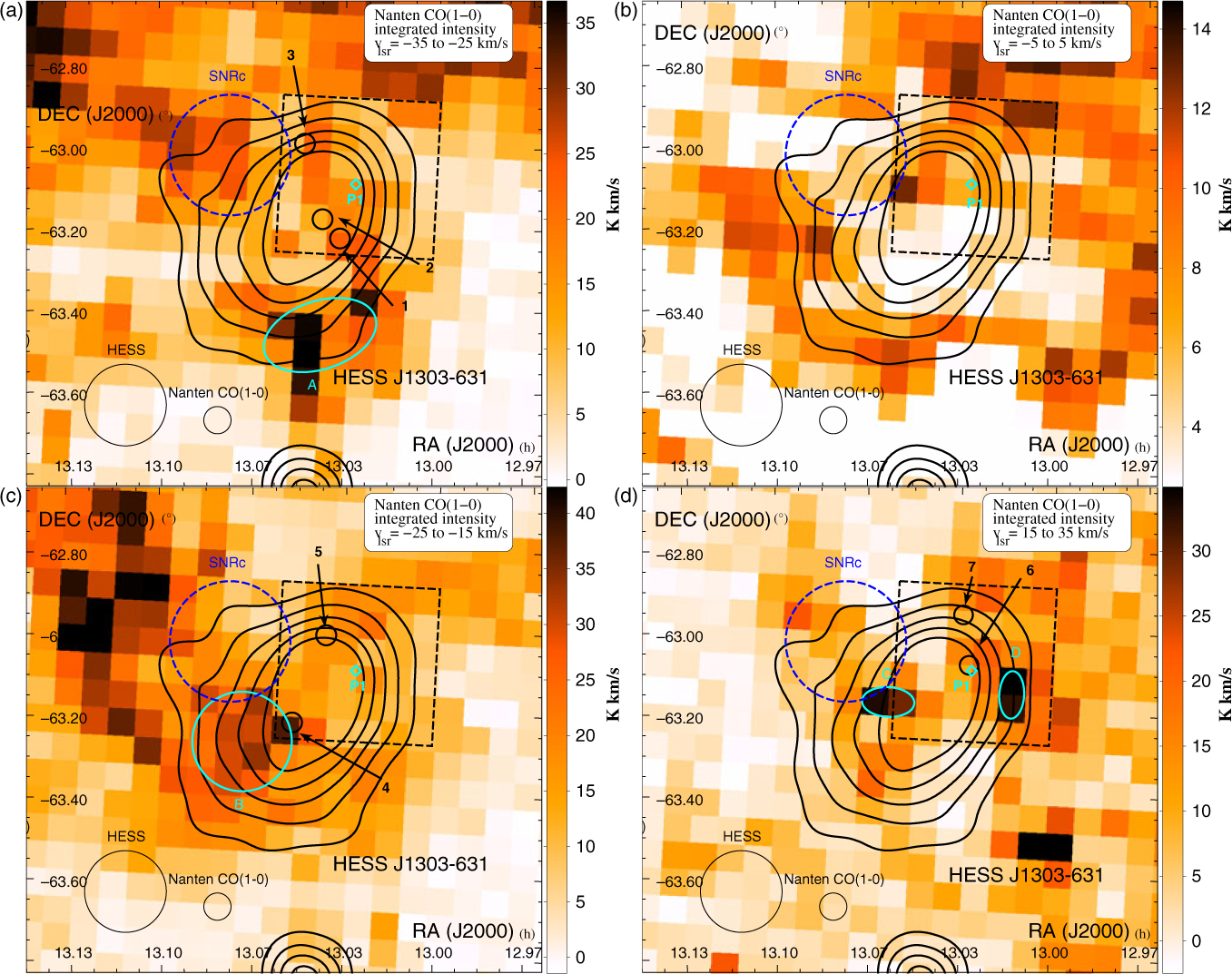
Figure 8. Nanten CO(1–0) integrated intensity map towards HESS J1303–631 (shown in black contours) between v slr = −35 to −25 km/s, −25 to −15 km/s, −5 to +5 km/s, and 15 to 35 km/s. The 7-mm map is shown as a black-dashed box, while the position and size of the SNR candidate from Sushch et al. (Reference Sushch, Oya, Schwanke, Johnston and Dalton2017) is indicated by a blue dashed circle. The position of the pulsar PSR J1301–6305 (P1) is shown in cyan diamond. The regions labelled ‘1’ to ‘7’ where CS(1–0) was detected are shown in black circles. The positions of prominent CO detections slightly overlapping the TeV emission are shown in cyan ellipses.
Based on the dispersion measure of this pulsar, Cordes et al. (Reference Cordes, Lazio, Chatterjee, Arzoumanian and Chernoff2002) suggested a distance d ∼ 6.6 kpc, much closer than the previous distance d ∼ 12.6 kpc (Taylor and Cordes Reference Taylor and Cordes1993). From the Nanten CO(1–0) components identified (see Figure 9), we focus on several molecular complexes in the line of sight at v lsr = −35 to −25 km/s (distance d ∼ 6.6 kpc, Scutum Crux arm), v lsr = −25 to −15 km/s (distance d ∼ 1.5 kpc, near Sagittarius–Carina arm), v lsr = −5 to 5 km/s (d ∼ 0.1 kpc, local arm) and v lsr = 25 to 35 km/s (distance d ∼ 12.6 kpc, far Sagittarius–Carina arm) shown in Figure 8. From our 7-mm CS observations, which cover the north-west part of the SNR towards the TeV source, we have identified several molecular clumps, which we have labelled ‘1 to 7’ (see Tables C.5 and D.4 for their physical parameters) but no extended CS(1–0) emission has been detected.
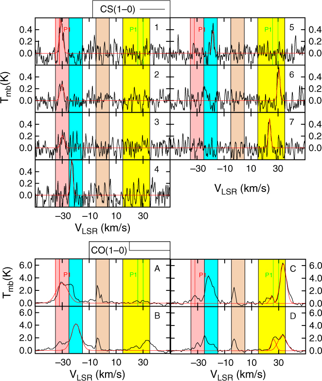
Figure 9. The averaged CS(1–0) and CO(1–0) emission from the different regions shown in Figure 8 towards HESS J1303–631. The red lines indicate the fit used to parametrise the emission. The fit parameters are displayed in Table C.5. Finally, the red and green vertical lines represent the dispersion measure distance of the pulsar P1 as predicted by Cordes et al. (Reference Cordes, Lazio, Chatterjee, Arzoumanian and Chernoff2002) and Taylor and Cordes (Reference Taylor and Cordes1993), respectively. The pink, cyan, brown, and yellow regions indicate the velocity range of the integrated intensity maps shown in Figure 8.
At all the aforementioned velocity ranges, it appears that some CO(1–0) emission always overlaps the TeV emission. It should be noted that the CO emission peaks south of HESS J1303–631 inside region ‘A’ at v lsr = −35 to −25 km/s. At the local arm (v lsr = −5 to 5 km/s), most of the CO(1–0) emission is distributed north east of the TeV source. At v lsr = 15 to 35 km/s, prominent CO emission is found overlapping HESS J1303–631 (see regions ‘C’ and ‘D’). We also note that the CO(1–0) emission does overlap the position of the SNR candidate represented in blue circle in Figure 8 at v lsr = −35 to −25 km/s and v lsr = 15 to 35 km/s.
Interestingly, we have found a CO(1–0) emission dip at v
lsr = −25 to −15 km/s localised towards the SNR candidate. From the position–velocity plots shown in Figure 10, we observe prominent CO emission which in fact appears to surround the SNR position (whose boundaries are shown in red dashed lines in Figure 10 bottom panels) between v
lsr = −22 to −15 km/s. From the CO(1–0) integrated intensity region at this velocity range, we also observe little spatial overlap between the molecular gas and the SNR candidate. Consequently, it may highlight the presence of a putative molecular shell at d ∼ 1.5 kpc coincident with the recently observed SNR candidate. The green cross and ellipse in Figure 10 indicate the position and the expansion speed (v
exp ∼ 4 km/s) of the putative molecular shell surrounding the SNR candidate. From the dashed magenta circular region in Figure 10 centred towards the SNR candidate position, the maximum mass swept by the SNR candidate reaches $M_{\textrm{H}_2}=3.3\times10^{4}{\textrm{M}_{\odot}}$
. We obtain as a upper limit a required kinetic energy
$M_{\textrm{H}_2}=3.3\times10^{4}{\textrm{M}_{\odot}}$
. We obtain as a upper limit a required kinetic energy $E_{\textrm{kin}}=1/2M_{\textrm{H}_2}v_{\textrm{exp}}^{2}=5.1\times10^{47}$
erg which represents ∼0.05% of the total kinetic energy from powerful O stars stellar winds over 1-Myr time-scale (see Weaver et al. Reference Weaver, McCray, Castor, Shapiro and Moore1977 for detailed study on interstellar bubbles). Consequently, the molecular shell may have been produced by the SNR progenitor star. We thus suggest this new SNR candidate is at distance at d ∼ 1.5 kpc, supporting its non-physical association with PSR J1301–6305 claimed by Sushch et al. (Reference Sushch, Oya, Schwanke, Johnston and Dalton2017).
$E_{\textrm{kin}}=1/2M_{\textrm{H}_2}v_{\textrm{exp}}^{2}=5.1\times10^{47}$
erg which represents ∼0.05% of the total kinetic energy from powerful O stars stellar winds over 1-Myr time-scale (see Weaver et al. Reference Weaver, McCray, Castor, Shapiro and Moore1977 for detailed study on interstellar bubbles). Consequently, the molecular shell may have been produced by the SNR progenitor star. We thus suggest this new SNR candidate is at distance at d ∼ 1.5 kpc, supporting its non-physical association with PSR J1301–6305 claimed by Sushch et al. (Reference Sushch, Oya, Schwanke, Johnston and Dalton2017).
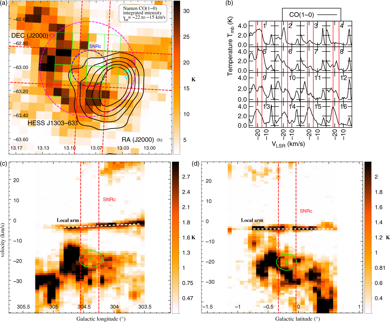
Figure 10. (panel a) Nanten CO(1–0) integrated intensity between v lsr = −22 to −15 km/s overlaid by the HESS TeV contours in black. The blue dashed circle indicates the size of the candidate SNR (Sushch et al. Reference Sushch, Oya, Schwanke, Johnston and Dalton2017). The cyan diamond shows the position of the pulsars PSR J1301–6305 (P1). The purple dashed circle indicates the region used to compute the mass of the putative molecular shell (see discussion in Section 4). The green grid of boxes indicates the position of the displayed CO(1–0) spectral lines (panel b). (panels c and d) Galactic longitude-velocity (l, v) and latitude-velocity (b, v) images integrated between l = [304.25°:304.55°] and b = [–0.34°:–0.04°], respectively (shown as red dashed lines in top left panel). The green cross-hair and ellipse show the location of a putative expanding molecular shell while the red dashed lines indicate the boundaries of the candidate SNR.
3.6. HESS J1018–589
HESS J1018–589 was first reported by Abramowski et al. (Reference Abramowski2012a) and actually consists of two distinct sources. The gamma-ray binary 1FGL J1018.6–5856 appears to be responsible for the HESS J1018–589A TeV emission (Abramowski et al. Reference Abramowski2012a), while HESS J1018–589B (shown in dashed black circle in Figure 11) is thought to be a PWN powered by the pulsar PSR J1016–587 (shown by a cyan diamond), with a rotation period P = 107 ms, a spin down energy $\dot{E}_{\textrm{SD}}=2.6\times10^{36}$
erg, and a characteristic age τ
c = 21 kyr (Camilo et al. Reference Camilo2001). It has been suggested that the pulsar, with dispersion measure distance d = 8 kpc, is not associated with the nearby SNR G292–1.8 located at d ∼ 2.9 kpc (Ruiz & May Reference Ruiz and May1986).
$\dot{E}_{\textrm{SD}}=2.6\times10^{36}$
erg, and a characteristic age τ
c = 21 kyr (Camilo et al. Reference Camilo2001). It has been suggested that the pulsar, with dispersion measure distance d = 8 kpc, is not associated with the nearby SNR G292–1.8 located at d ∼ 2.9 kpc (Ruiz & May Reference Ruiz and May1986).
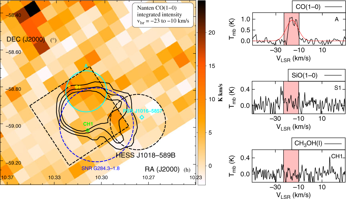
Figure 11. Nanten CO(1–0) integrated intensity map towards HESS J1018–589 between v lsr = −23 to 10 km/s overlaid by the TeV gamma-ray emission from HESS 1018–589 in solid black contours. The dashed black circle indicates the size and position of HESS J1018–589B. The SNR G284.3–01.8 is shown as a blue dashed circle, while the pulsar PSR J1019–5857 is shown as a cyan diamond. The extended CO region labelled ‘A’ is shown in cyan, the position of the SiO(1–0, v = 0) ‘S1’ are displayed in yellow, and the CH3OH maser found in the region ‘CH1’ is shown in green. Their respective spectral lines are displayed on the right-hand side. The pink region illustrates the aforementioned velocity range.
From the Nanten CO(1–0) observations shown in Figure 11, we have identified CO emission at v
lsr = −23 to −10 km/s, inferring a near distance d ∼ 2.8 kpc, matching the SNR distance. The CO(1–0) emission appears filamentary north of HESS J1018–589B and partially overlaps the northern rim of SNR G292–1.8. The molecular gas in region ‘A’, with mass attaining $M_{\textrm{H}_2}\left(\textrm{CO}\right)=2.9\times10^{3}{\textrm{M}_{\odot}}$
, shows quite broad emission (Δv ∼ 12 km/s, see Table C.6 and Figure 11). Although no CO emission was revealed at v
lsr ∼ 30 km/s, we note from Figure E.3 significant Hi emission, which may suggest that the ISM surrounding HESS J1018–589B mostly consists of atomic gas.
$M_{\textrm{H}_2}\left(\textrm{CO}\right)=2.9\times10^{3}{\textrm{M}_{\odot}}$
, shows quite broad emission (Δv ∼ 12 km/s, see Table C.6 and Figure 11). Although no CO emission was revealed at v
lsr ∼ 30 km/s, we note from Figure E.3 significant Hi emission, which may suggest that the ISM surrounding HESS J1018–589B mostly consists of atomic gas.
4. Discussion of gamma-ray emission
In this section, we use results from our ISM studies to discuss whether the CRs and/or high energy electrons interacting with the ISM can contribute to the TeV emission or at least affect their morphology. In this section, we first introduce the method used to check whether hadronic CRs could contribute to the observed TeV emission. Then, we will briefly indicate how leptonic emission can also be affected by the ISM.
4.1. TeV emission from CRs
Based on the mass estimates towards molecular regions overlapping the TeV sources, we use eq. 10 from Aharonian (Reference Aharonian1991) to derive the CR enhancement factor k CR = w CR/w ⊙ which represents the ratio between w CR the energy density of CRs towards an MC next to a TeV source, and w ⊙ ∼ 1.0 eV cm−3 the energy density found in the solar neighbourhood. We use the combined atomic and molecular mass to obtain the total amount of target material available. Table 2 indicates the k CR values required for each molecular regions (partially) overlapping the TeV sources to account for the observed TeV fluxes. The k CR value can then be compared to typical CR enhancement factors predicted in the vicinity of SNRs (and potentially towards PWNe) to check the plausibility of hadronic contribution.
Table 2. Cosmic-ray enhancement factors k
cr derived using eq. 10 from Aharonian (Reference Aharonian1991), required to reproduce the observed TeV emission above 1 TeV $F(\gt 1\,{\rm TeV}) = \int N_0 E_{\gamma}^{-\Gamma}{\rm d}{E}_{\gamma}$
via CR–ISM interaction.
$F(\gt 1\,{\rm TeV}) = \int N_0 E_{\gamma}^{-\Gamma}{\rm d}{E}_{\gamma}$
via CR–ISM interaction.
*Aharonian et al. (Reference Aharonian2007), †Abramowski et al. (Reference Abramowski2011), ‡Abdalla et al. (Reference Abdalla2018a), ±, ∐ Aharonian et al. (Reference Aharonian2006), Abramowski et al. (Reference Abramowski2012b), *Abramowski et al. (Reference Abramowski2015)
a We scaled down the HESS J1809–193 photon flux by 16%, 16% and 12% for regions ‘1’, ‘2’, ‘3’, respectively, corresponding to the ratio between the molecular regions and the TeV emission sizes.
b We scaled down the HESS J1420–607 photon flux by 4%, ∼1%, <1%,, 1%, and 3% for the regions 6 to 10, respectively.
c We scaled down the HESS J1303–631 photon flux by 44%, 7% and 7% for region ‘A’, ‘B’, and ‘C’, respectively.
4.1.1. Contribution from nearby SNRs?
Nearby SNRs are the most likely viable candidates to produce CRs energy densities up to ∼103 eV cm−3 (see Reynolds Reference Reynolds2008 and references therein). CRs propagate along the magnetic field lines and they scatter from their interaction with magnetic field perturbations (provided the scale of the perturbation roughly equals the CR gyroradius). As the magnetic field turbulence is thought to be enhanced in MCs, we here assume an isotropic diffusion of CRs and electrons as a first-order approximation. If we assume an isotropic diffusion of CRs and neglect energy losses, we can estimate the energy density distribution of CRs at a distance R from the SNR (here assumed as an impulsive source of CRs; see Aharonian & Atoyan Reference Aharonian and Atoyan1996):
 $$\begin{align} n\left(E,R,t\right)&=\frac{\eta_{\textrm{pp}}E_\textrm{SNR}}{\left(m_\textrm{p}c^2\right)^{2-\alpha}}\frac{E^{-\alpha}}{\pi^{3/2} R_\textrm{d}^{3}}\exp\left(-\left(\frac{R}{R_\textrm{d}}\right)^2\right) \end{align}
 $$\begin{align} R_\textrm{d}&=2\left(\chi D_{10}t_\textrm{age}\sqrt{E/10\textrm{ GeV}}\right)^{1/2}\end{align}
with m p being the proton mass, D 10 = 1028 cm2s−1 being the diffusion coefficient of 10 GeV CRs, α the spectral index of the proton distribution, and η pp the ratio of the total SNR energy E SNR transferred to CRs. R d(t) represents the diffusion radius travelled by CRs after a time t. The diffusion suppression factor χ accounts for slower diffusion of particles which can be caused, for instance, by streaming instabilities or perturbations caused by shocks (see Nava et al. Reference Nava, Gabici, Marcowith, Morlino and Ptuskin2016; Malkov et al. Reference Malkov, Diamond, Sagdeev, Aharonian and Moskalenko2013, and references therein). Here we use, χ = 0.01 to 1 which matches the slow and fast diffusion coefficient regimes defined by Aharonian & Atoyan (Reference Aharonian and Atoyan1996). Various studies of the CRs interacting with nearby molecular clouds W 28 (Giuliani et al. Reference Giuliani2010; Li & Chen Reference Li and Chen2010; Gabici et al. Reference Gabici, Casanova, Aharonian, Rowell, Boissier, Heydari-Malayeri, Samadi and Valls-Gabaud2010) have, in fact, suggested a suppression factor between χ = 0.01 and 0.1. However, the value of χ remains poorly constrained. From Eq. 1, we can then obtain the total energy density of CRs w CR(R, t) using the following equation:
 $$\begin{equation} w_\textrm{CR}\left(R,t\right)=\int_{\epsilon_0}{n\left(E,R,t\right)E\textrm{d}E} \label{getenergy}\end{equation}
where ε 0 = m p c 2 is the proton energy at rest. Figure 12 illustrates the range of k CR produced by SNRs with initial energy E SNR = 1051 erg as a function of the SNR age, using a standard proton spectral index α = 2.2 and η pp = 0.1. From the distance between the SNRs and the surrounding ISM regions (see Table 2), and the age of the SNRs, we can then check whether the required enhancement factors from Table 2 fall within the predicted range from nearby SNRs.
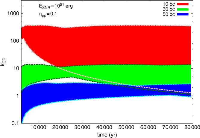
Figure 12. Evolution of the cosmic-ray enhancement factor k CR range as a function of time at a distance d = 10 pc (red), d = 30 pc (green), and d = 50 pc (blue) away from an impulsive source with initial energy E SNR = 1051 erg and initial CR spectral index α = 2.2. A energy-dependent diffusion of CRs (see Section 4) has been applied with a diffusion coefficient at 10 GeV bounded between D 10 = 1025 to 1028 cm2 s−1.
4.1.2. CR contribution from PWNe?
Additionally, a few authors (see Amato Reference Amato2014 and references therein) have also argued that high energy hadrons could also be produced inside the pulsar environment, and be responsible for several features inside the PWN (e.g. wisps in the Crab PWN; Gallant Arons Reference Gallant and Arons1994). Providing high energy CRs have indeed been produced inside PWNe and not suffered heavy adiabatic losses, we will thus discuss whether the pulsars considered in this work could also generate the required CR enhancement factors shown in Table 2. In order to model the high CR energy density potentially produced by those pulsars, we account for the evolution of the spin down power $\dot{E}_\textrm{SD}$
as a function of time t, which can be described as follows:
$\dot{E}_\textrm{SD}$
as a function of time t, which can be described as follows:
 $$\begin{eqnarray} &\dot{E}_\textrm{SD}\left(t\right)=\dot{E}_\textrm{SD}\left(t_\textrm{age}\right)\left(1+\left(n_\textrm{b}-1\right)\frac{\dot{P}\left(t-t_\textrm{age}\right)}{P}\right)^{-\Gamma} \end{eqnarray}
 $$\begin{eqnarray} &\Gamma=\frac{n_\textrm{b}+1}{n_\textrm{b}-1} \end{eqnarray}
with t
age being the current age of the PWN, P(t) and $\dot{P}\left(t\right)$
being the current period and period derivative of a pulsar, respectively, at time t,
$\dot{P}\left(t\right)$
being the current period and period derivative of a pulsar, respectively, at time t, $\dot{E}_\textrm{SD}\left(t\right)$
being the pulsar spin down power at time t, and n
b being the pulsar braking index. In order to obtain the density of CRs at a given radius R from the pulsar, we rewrite Eq. 1 using the source term
$\dot{E}_\textrm{SD}\left(t\right)$
being the pulsar spin down power at time t, and n
b being the pulsar braking index. In order to obtain the density of CRs at a given radius R from the pulsar, we rewrite Eq. 1 using the source term $S\left(t\right)=\eta_\textrm{pp}\dot{E}_\textrm{SD}\left(t\right)/\left(m_\textrm{p}c^2\right)^{2-\alpha}$
, with η
pp being the fraction of the spin down power transferred to CRs. We thus numerically solve the following equation:
$S\left(t\right)=\eta_\textrm{pp}\dot{E}_\textrm{SD}\left(t\right)/\left(m_\textrm{p}c^2\right)^{2-\alpha}$
, with η
pp being the fraction of the spin down power transferred to CRs. We thus numerically solve the following equation:
 $$ \begin{equation} n\left(E,R,t\right)=\frac{E^{-\alpha}}{\pi^{3/2}}\int_{t_\textrm{age}}^{0}{-\frac{S\left(\xi-t_\textrm{age}\right)}{R_d^3\left(\xi\right)}\exp\left(-\frac{R^2}{R_d^2\left(\xi\right)}\right)\textrm{d}\xi} \label{diffusionpulsar} \end{equation}
with ξ = t age − t. As per the SNR scenario, we obtain the CR energy density at a given distance R from pulsar using Eq. 3.
Figure 13 illustrates the CR energy density produced by the various pulsars as a function of the diffusion coefficient suppression factor χ. Here, we assumed n b = 3 for all pulsars, except for PSR J1119–6127 in which we used the measured braking index n b = 2.68. From the spectral modelling towards several PWNe, Bucciantini, Arons & Amato (Reference Bucciantini, Arons and Amato2011) suggested that the maximum energy rate available to be transferred to CRs must be at most 0.20 of the total spin down power. We thus have used η pp= 0.20 and the k CR values shown in Figure 13 are consequently upper limits. In the following subsections, we compare these predictions with the various required k CR (see Table 2) derived inside the molecular regions.
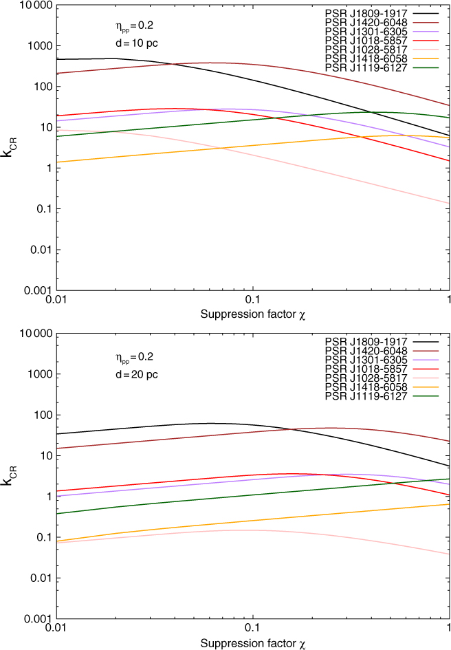
Figure 13. Predicted energy density k CR from pulsars at 10 pc (top panel) and at 20 pc (bottom panel) distance as a function of the diffusion coefficient suppression factor χ (see colour version online).
4.2. TeV emission from high energy electrons
As opposed to CRs, high energy electrons suffer heavy radiation losses as they diffuse inside the dense ISM because of the potentially enhanced magnetic field strength (see Crutcher et al. Reference Crutcher, Wandelt, Heiles, Falgarone and Troland2010). In the lack of intense radiation fields, synchrotron losses, with time-scale $\tau_{\textrm{sync}}=2.45\times10^{7}\big(B^2_{\textrm{mg}}E/m_\textrm{e}c^2\big)^{-1}$
yr (B
mg = B/1mG being the magnetic field strength and E being the total energy of the electron), are likely to dominate over IC losses inside MCs. Although Bremsstrahlung emission, with time-scale τ
brem ∼ 4.6 × 10⁷(n/1 cm−3)−1 yr, may contribute inside MCs with densities n
H > a few × 103 cm−3 in the 0.1 to 1 TeV band, we expect the TeV emission above 1 TeV to anti-correspond with the molecular ISM as the IC radiation is likely to dominate above 1 TeV. Table 3 indicates the synchrotron energy loss time-scale τ
sync for electrons with energy E = 10 TeV, required to produce photons with energy Eγ
∼ 1 TeV. To obtain B values inside MCs, we use the Crutcher et al. (Reference Crutcher, Wandelt, Heiles, Falgarone and Troland2010) relation:
$\tau_{\textrm{sync}}=2.45\times10^{7}\big(B^2_{\textrm{mg}}E/m_\textrm{e}c^2\big)^{-1}$
yr (B
mg = B/1mG being the magnetic field strength and E being the total energy of the electron), are likely to dominate over IC losses inside MCs. Although Bremsstrahlung emission, with time-scale τ
brem ∼ 4.6 × 10⁷(n/1 cm−3)−1 yr, may contribute inside MCs with densities n
H > a few × 103 cm−3 in the 0.1 to 1 TeV band, we expect the TeV emission above 1 TeV to anti-correspond with the molecular ISM as the IC radiation is likely to dominate above 1 TeV. Table 3 indicates the synchrotron energy loss time-scale τ
sync for electrons with energy E = 10 TeV, required to produce photons with energy Eγ
∼ 1 TeV. To obtain B values inside MCs, we use the Crutcher et al. (Reference Crutcher, Wandelt, Heiles, Falgarone and Troland2010) relation:
 $$\begin{eqnarray} & B=10\,\mu\textrm{G} & \textrm{for } n_{\textrm{H}} \lt 300\,\textrm{cm}^{-3} \end{eqnarray}
 $$\begin{eqnarray} & B=10\left(\dfrac{n_{\textrm{H}}}{300\textrm{ cm}^{-3}}\right)^{0.6}\,\mu\textrm{G} &\textrm{for } n_{\textrm{H}}\ge300\,\textrm{cm}^{-3}. \end{eqnarray}
We compare these time-scales with the age of nearby high energy sources and the diffusion time-scale τ
diff required for the particles with energy above 10 TeV to fully cross a molecular region. We here define τ
diff = (〈r〉 + d
source)2/6D (E, B, χ), with 〈r〉 being the mean radius of the molecular region and d
source being the distance separating the centre of the high energy source to the centre of the molecular region. To check the leptonic scenario, we first select dense molecular regions which anti-correspond with each TeV source and/or its X-ray counterpart. Here, we preferably use the extended CS regions as most of the observed gas is confined. However, in the cases where no CS(1–0) emission was detected (i.e. HESS J1018–189B, HESS J1303–631, and HESS J1119–164), we use the CO regions. We again note that the densities $n_{\textrm{H}_2}$
from our CO analyses are upper limits. Thus, these synchrotron time-scale values should be, in these cases, used as upper limits. Then, we derive the synchrotron time-scale and compare it to τ
diff required for the high energy electrons to cross the cloud. In the case where the synchrotron time-scale is much smaller than the diffusion time-scale, we expect the high energy electrons to radiate most of their energy and thus become unable to produce X-rays and TeV emission inside the MC. An anti-correlation between the ISM and X-rays would support the physical connection between the TeV source and the ISM as well as the leptonic nature of the TeV source (see Sano et al. Reference Sano2013).
$n_{\textrm{H}_2}$
from our CO analyses are upper limits. Thus, these synchrotron time-scale values should be, in these cases, used as upper limits. Then, we derive the synchrotron time-scale and compare it to τ
diff required for the high energy electrons to cross the cloud. In the case where the synchrotron time-scale is much smaller than the diffusion time-scale, we expect the high energy electrons to radiate most of their energy and thus become unable to produce X-rays and TeV emission inside the MC. An anti-correlation between the ISM and X-rays would support the physical connection between the TeV source and the ISM as well as the leptonic nature of the TeV source (see Sano et al. Reference Sano2013).
Table 3. The diffusion time-scale t diff = (〈r〉 + d source)2/6D(E, B) for a particle with energy E = 10 TeV to cross the listed molecular regions with mean radius 〈r〉 and positioned at d source from the centre of the listed sources. The age of the source t age, the CR–ISM interaction time-scale τ pp for protons, and the synchrotron time scale τ sync for electrons with energy E = 10 TeV are also displayed as means of comparison.
a Obtained from eq. 21 from Crutcher et al. (Reference Crutcher, Wandelt, Heiles, Falgarone and Troland2010) (see Section 4.2).
b $\tau_{\rm pp} = 6 \times 10^{7}/2n_{{\rm H}_{2}}$
where
$\tau_{\rm pp} = 6 \times 10^{7}/2n_{{\rm H}_{2}}$
where $n_{{\rm H}_{2}}$
can be found in Tables D.1–D.6.
$n_{{\rm H}_{2}}$
can be found in Tables D.1–D.6.
c $\tau_{sync} = 2.45 \times 10^{7} (B^2_{mG}E/m_{e})^{-1}$
yr (Ginzburg & Syrovatskii Reference Ginzburg and Syrovatskii1964).
$\tau_{sync} = 2.45 \times 10^{7} (B^2_{mG}E/m_{e})^{-1}$
yr (Ginzburg & Syrovatskii Reference Ginzburg and Syrovatskii1964).
d See eqs. 2 and 3 from Gabici, Aharonian, Blasi (Reference Aharonian2007) to obtain the diffusion time-scale. The results shown assume a diffusion coefficient suppression factor χ = 0.1
e SNR candidate, see text and Sushch et al. (Reference Sushch, Oya, Schwanke, Johnston and Dalton2017) for further details and Figure 8 for location. We used standard SNR expansion parameters to provide an age estimate of the SNRc if located at this distance (see text).
4.3. Discussion of Individual Sources
4.3.1. HESS J1809–193
Castelletti et al. (Reference Castelletti, Giacani and Petriella2016), and more recently Araya (Reference Araya2018), have discussed the hadronic scenario in which they assume the SNR G011.0–0.0 to be located at a distance d ∼3.0 kpc. We focus here on how MCs at d ∼ 3.7 kpc can affect the TeV emission produced by the PWN powered by PSR J1809–1917 and SNR G011.0–0.0, in which we argue they are physically connected.
We remark in Table 3 that the synchrotron energy loss time-scale τ sync for electrons above 10 TeV is significantly smaller than the diffusion time-scale through the various ISM regions. Consequently, most electrons producing gamma-rays above 1 TeV would not penetrate the dense molecular regions.
We also check whether the CRs in MCs may produce significant TeV emission. To match the observed ISM regions, the TeV flux was scaled simplistically by area ratio, which is 16%, 16%, and 12% towards regions ‘1’, ‘2’, and ‘3’, respectively. We conclude that a CR enhancement factor k CR = 10 − 30 (see Table 2) is required to attain the TeV flux towards region ‘1’, ‘2’, and ‘3’, respectively. As the distances between these SNRs and the molecular regions range between 10 and 20 pc (see Table 3), we find, based on the red and green regions in Figure 12, that, at t age = 51 kyr, the predicted k CR ranges to be between k CR ∼ 1 and 300. Consequently, the SNR G011.0–0.0 may be able to produce the required CR enhancement and produce hadronic TeV emission. Interestingly, we find that the PWN powered by PSR J1809–1917 (see black line in Figure 13) could also significantly increase the predicted CR enhancement factor towards nearby MCs with k CR values peaking at ∼270 (for diffusion suppression χ = 0.02) and thus generally exceeds the aforementioned k CR towards the molecular regions ‘1’ and ‘2’. Although these CR energy densities should be considered as upper limits, the PWN powered by the PSR J1809–5158 may consequently be a viable laboratory to probe possible hadronic components originating from the PWN.
4.3.2. HESS J1026–583
It has already been stated that, based on energetics alone, the spin down energy of the pulsar PSR J1028–5819 could produce the HESS J1026–583 TeV emission (Abramowski et al. Reference Abramowski2011).
From our CO(1–0) and CS(1–0) data, we have however identified a dense molecular region spatially coincident with the TeV emission. If the TeV emission is indeed of hadronic origin, we also require a proton spectrum J(E) ∝ E −1.94 to generate the photon spectrum towards HESS J1026–583 (see Abramowski et al. Reference Abramowski2011).
Taking into account this hard gamma-ray spectra, the eq. 10 from Aharonian (Reference Aharonian1991) must be adjusted by a factor of 1.6/0.94 = 1.7. We thus obtain the CR enhancement factor k
cr = 60. Using the combined mass of the regions ‘5’ to ‘7’ $M_{\textrm{H}_2}\left(\textrm{CS}\right)=5.0\times10^{3}{\textrm{M}_{\odot}}$
, the required CR enhancement factor only increases to k
CR = 103. We find that this value can only be attained if there is an SNR located art d < 10 pc to the molecular region ‘B’ (see red region in Figure 12). However, no SNRs nor any CR accelerators have been detected close to this MC so far.
$M_{\textrm{H}_2}\left(\textrm{CS}\right)=5.0\times10^{3}{\textrm{M}_{\odot}}$
, the required CR enhancement factor only increases to k
CR = 103. We find that this value can only be attained if there is an SNR located art d < 10 pc to the molecular region ‘B’ (see red region in Figure 12). However, no SNRs nor any CR accelerators have been detected close to this MC so far.
4.3.3. HESS J1119–164
The centroid of the TeV emission appears to be located north-west of PSR J1119–6127, towards regions ‘X1’ and ‘X2’. The non-thermal X-ray emission, thought to be produced by high energy electrons inside the front shock, is unlikely to have also produced the TeV emission. The possible cause of the TeV gamma-ray emission may either come from high energy electrons from the PWN, or the CRs produced by the SNR front shock as they interact with the ISM in region ‘D’. By modelling the GeV and TeV spectral energy distribution using Fermi-LAT and HESS data, respectively, Acero et al. (Reference Acero2013) showed that electrons originating from the PWN could reproduce the observed spectrum. The offset of the TeV emission with respect to the pulsar position could suggest that the PWN may have been crushed by the reverse shock of the progenitor SNR. The Nanten CO(1–0) survey has however not revealed any significant emission east of PSR J1119–6127 between v lsr = 20 to 40 km/s. A higher resolution gas survey could resolve clumps which could be responsible for the asymmetry.
The hadronic scenario may also be plausible as the TeV gamma-ray emission corresponds with the CO(1–0) emission west of SNR G292.2–0.5. The thermal X-ray emission towards region ‘D’ suggest that some of the gas in region ‘D’ may have been heated as it interacted with the SNR. From Table 2, the required CR enhancement factor k CR required for the CRs to produce the TeV gamma-ray flux is ∼ 143. An SNR age t = 1.9 kyr suggests that the bulk of CRs are remained confined inside the SNR front shock. However, the steep photon spectral index Γ = 2.64 above 1 TeV (Abdalla et al. Reference Abdalla2018a) also indicates that CRs above 10 TeV have already escaped the SNR. With the increased sensitivity of CTA, one could look at the spatial and spectral evolution of the TeV gamma-ray emission inside the ISM towards region ‘D’. A hardening of the TeV gamma-ray spectrum with increasing distance of the SNR could favour the hadronic scenario.
Finally, as shown by the orange line in Figure 13, we also find that the pulsar is unlikely to have produced enough CRs to produce the TeV emission towards HESS J1119–164.
4.3.4. HESS J1418–609 and HESS J1420–607
From Table 2, we observe k CR values ranging between 50 and 90 towards the clumps ‘6’ to ‘10’, whose projected distance ranges between 22 pc and 35 pc (see Table 3). Assuming the progenitor SNR of PSR J1418–6058 is 1.6 kyr old, we note that escaping CRs are unlikely to produce significant TeV gamma-ray emission towards HESS J1420–607 (see blue region in Figure 12). As per HESS J1119–164, it is expected that CRs may still remain confined inside the SNR front shock. Similarly for the leptonic scenario (see Table 3), a fast diffusion coefficient (χ > 0.1) is required for electrons to reach the clumps ‘6’ to ‘10’ and the gas in region ‘A’. Kishishita et al. (Reference Kishishita, Bamba, Uchiyama, Tanaka and Takahashi2012) indicated that a slow diffusion of electrons inside the PWNe is required to produce the diffuse X-ray emission observed with Suzaku. Consequently, it is unlikely that high energy electrons escaping HESS J1418–609 can contribute to the TeV emission towards HESS J1420–607.
The various clumps north of HESS J1418–609 could affect its TeV emission. From Table 3, we note that, although some clumps could impede the propagation of multi-TeV electrons (τ sync ≪ τ diff), a large diffusion coefficient would also be necessary for the high energy electrons to reach these clumps. Consequently, at this distance, the effect of the ISM on the morphology of HESS J1418–609 is also not significant.
4.3.5. HESS J1303–631
HESS J1303–631 has clearly been identified as a PWN based on energy dependent morphology at TeV energies (Abramowski et al. Reference Abramowski2012b). We here check the potential contribution of the molecular regions ‘A’ to ‘D’ to the observed TeV gamma-ray emission.
From Table 3, we find that, assuming a suppression factor χ = 0.1, high energy electrons would only reach the molecular regions ‘A’ (located at d ∼ 6 kpc) and ‘C’0.3pt, ’D’ (both located at d ∼ 13.6 kpc). In all cases, the shorter synchrotron time-scale indicates that any high energy electrons would lose most of their energy while diffusing into these molecular regions. Consequently, if associated with the PWN, less TeV emission spatially overlapping with these molecular regions should be expected.
Now, we discuss whether the selected molecular regions can also affect the morphology of the TeV emission from hadronic interactions. As per the case of HESS J1809–193, we scaled down the photon flux of HESS J1303–631 to 44%, 7%, and 7% for regions ‘A’0.3pt, ‘C’, and ‘D’, respectively, based on the size ratio between the molecular regions and the TeV emission. We then obtain k CR ∼ 200 (see Table 2). Based on the distances between the MCs to the pulsar or SNR candidate (see Table 3), we find from Figures 12 and 13 that neither the pulsar (see purple line) nor the SNR candidate can provide sufficient CR energy density to produce hadronic TeV emission.
4.3.6. HESS J1018–589
We now discuss how the ISM in region ‘A’ may affect the TeV emission towards HESS J1018–589a. We find that the enhancement factor k CR = 91 (see Table 2) is required for the CR to produce observed TeV flux. A 10-kyr-old SNR is capable of producing such CR enhancement if the distance between the SNR and the cloud is ∼ 10 pc (see red region in Figure 12). A lack of TeV emission coincident with the region ‘A’ may suggest that the MC may be foreground/background to the SNR and thus may not be physically connected. Here we discuss only the possible contribution from CRs originating from the SNR G284.3–1.8. From our mass estimate in region ‘A’ (see Table C.6), we find that a slow diffusion of CRs escaping the SNR might lead to a significant contribution of the hadronic TeV emission towards HESS J1018–583A.
5. Conclusion
In this paper, we have mapped the molecular and atomic ISM towards PWNe and PWN candidates, combining our new 7-mm Mopra survey with the Nanten CO(1–0) data and the SGPS/GASS Hi survey. Except for the cases of HESS J1303–631 and HESS J1018–589B, our ISM studies provided additional information about the distance of astrophysical sources potentially related to the TeV source. We have also identified MCs which could explain the morphology of the TeV gamma-ray emission as observed by CTA (Acharya et al. Reference Acharya2013), and also highlight CRs originating from progenitor supernova remnants (SNRs). From the hypothesis that CRs could also be produced within the pulsar environment, and that at most 20% of the spin down power could be transferred to CRs (Bucciantini et al. Reference Bucciantini, Arons and Amato2011), we find that, among the studied PWNe, only CRs from PSR J1809–1917 could contribute to the TeV emission.
Towards HESS J1809–193, we have found several dense molecular regions at v
lsr = 10 to 22 km/s and v
lsr = 25 to 38 km/s adjacent to the pulsar PSR J1809–1918 and the SNRs G011.0–0.0 and G011.1+0.1. Notably, we have detected SiO(1–0) emission towards the dense MC south of HESS J1809–193 with no IR counterparts, suggesting a possible SNR-MC interaction at the pulsar dispersion measure distance d ∼ 3.7 kpc. We found that the ambient density required to reconcile the projected radius of SNR G011.0–0.0 with the characteristic age of the pulsar PSR J1809–1917 is consistent with the averaged density $n_{\textrm{H}_2}$
obtained from our CO analysis. We argue that the PWN electrons could lose most of their energy before propagating deep inside the nearby MCs, and would therefore become unable to produce coincident TeV gamma-ray emission. We also note that the CRs that have escaped the pulsar’s progenitor SNR may produce significant TeV emission towards these MCs.owards HESS J1026–582, the MCs east of the pulsar PSR J1028–5819 may explain its offset position with respect to the peak of the TeV emission at d ∼ 2.7 kpc. However, we have also found a partial shell structure spatially coincident with the TeV emission at d ∼ 5 kpc and highlight a potential hadronic origin, powered by an unknown CR source at d < 10 pc from the MC.
$n_{\textrm{H}_2}$
obtained from our CO analysis. We argue that the PWN electrons could lose most of their energy before propagating deep inside the nearby MCs, and would therefore become unable to produce coincident TeV gamma-ray emission. We also note that the CRs that have escaped the pulsar’s progenitor SNR may produce significant TeV emission towards these MCs.owards HESS J1026–582, the MCs east of the pulsar PSR J1028–5819 may explain its offset position with respect to the peak of the TeV emission at d ∼ 2.7 kpc. However, we have also found a partial shell structure spatially coincident with the TeV emission at d ∼ 5 kpc and highlight a potential hadronic origin, powered by an unknown CR source at d < 10 pc from the MC.
Towards HESS J1119–164, the MCs at the kinematic distances d ∼ 8.6 to 9.7 kpc found on the west side of SNR 292.2–0.5 show good correspondence with the thermal X-ray detections with Chandra and XMM-Newton, suggesting a possible SNR-MC interaction. Our comparative study of our column density estimates with the column density derived from X-ray measurements also supports the TeV source distance d > 8.6 kpc.
Combining our column density study as well as our ISM morphology study towards HESS J1418–609, we argue the TeV source may be located at d ∼ 3.5 − 5.6 kpc. We also claim that the various molecular clumps are too far from the pulsar PSR J1418–6058 to affect or contribute to the TeV gamma-ray emission.
Our ISM analysis has not constrained the distance of HESS J1303–631 as the CO(1–0) emission overlaps the TeV emission at all velocity ranges. Notably, at v lsr = −22 to −15 km/s, however, we did find a CO dip spatially coincident with the SNR candidate found by Sushch et al. (Reference Sushch, Oya, Schwanke, Johnston and Dalton2017), inferring a distance d ∼ 1.5 kpc.
Although CO(1–0) emission north of the SNR G284.3–1.8 towards HESS J1018–589 has been found at d ∼ 2.8 kpc, no CS clumps have been found at the pulsar PSR J1019–5857 dispersion measure distance d ∼ 8.6 kpc, suggesting an atomic-dominated ISM surrounding HESS J1018–589B. An extension of high resolution Hi survey would shed more light concerning this TeV source.
As a conclusion, the arc-minute structure of the ISM plays an important role in understanding the morphology of the TeV gamma-ray emission produced by PWNe and progenitor SNR. The angular resolution and sensitivity of the Mopra CO(1–0) and 13CO surveys (Braiding et al. Reference Braiding2015) will refine the structure and dynamics of the diffuse molecular gas.
As future work, we aim to use the various properties of the identified clumps; to model the effect of the diffusion of CRs, and high energy electrons, escaping the PWNe and their progenitor SNRs; to model the interaction of these particles with the identified MC clumps; and to identify spectral and/or morphological signatures of the TeV gamma-ray emission. These could then be compared to upcoming observations with CTA (Acharya et al. Reference Acharya2013), which could further constrain the nature of the TeV sources.
Author ORCIDs
N. Maxted https://orcid.org/0000-0003-2762-8378
Acknowledgements
The Mopra radio telescope is part of the Australia Telescope National Facility which is funded by the Australian Government for operation as a National Facility managed by CSIRO. Operations support was provided by the University of New South Wales and the University of Adelaide. The University of New South Wales Digital Filter Bank used for the observations with the Mopra Telescope (the UNSWMOPS) was provided with support from the Australian Research Council LE160.100094 (ARC).
Appendix A. Cleaning and integrated intensity mapping methods
A flow chart which outlines the various processes used to clean the various data-cubes and produce improved integrated intensity maps is shown in Figure A.1. The procedure to produce clean data-cubes is explained in Section 2.
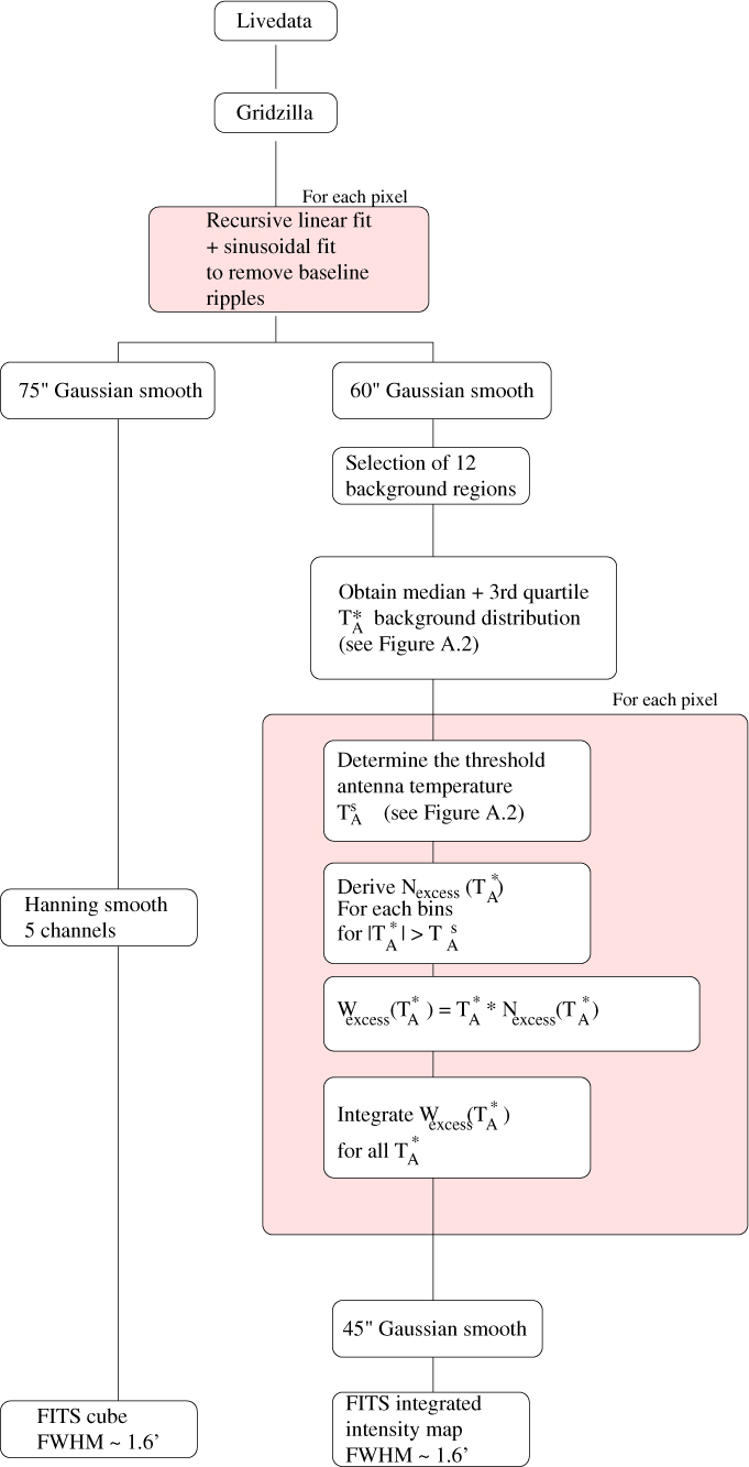
Figure A.1. Flow chart describing the procedure used to reduce our Mopra 7-mm observation data. The left path indicates the procedure used to create cleaned data-cubes, while the right paths shows the procedure to create integrated intensity maps.
A.1. Integrated intensity maps
From the unsmoothed cleaned data-cubes, we first apply a Gaussian smooth with FWHM∼1′ using the Miriad task Convol. Then, from our cleaned data-cubes, we choose 12 background regions, each consisting of nine pixels, across the map, with no CS(1–0) emission. From the spectra obtained from these background regions, a binned distribution of the number of channels $N_\textrm{ch}\left(T_\textrm{A}^{*}\right)$
within the antenna temperature
$N_\textrm{ch}\left(T_\textrm{A}^{*}\right)$
within the antenna temperature $T_\textrm{A}^{*}$
and
$T_\textrm{A}^{*}$
and $T_\textrm{A}^{*}+\Delta T_\textrm{A}^{*}$
is then plotted (
$T_\textrm{A}^{*}+\Delta T_\textrm{A}^{*}$
is then plotted ( $(\Delta T_\textrm{A}^{*}\,{=}\,0.01 \ K$
in this work). We then record the median N
ch value for each bin to obtain our background distribution (see purple histogram in Figure A.2). Note that we also record the third quartile of the background distribution (see error bars in Figure A.2) to look at the fluctuation of the background distribution. Now that we have estimated the background level distribution at the studied velocity range, the integrated intensity of each pixel is derived using the following method:
$(\Delta T_\textrm{A}^{*}\,{=}\,0.01 \ K$
in this work). We then record the median N
ch value for each bin to obtain our background distribution (see purple histogram in Figure A.2). Note that we also record the third quartile of the background distribution (see error bars in Figure A.2) to look at the fluctuation of the background distribution. Now that we have estimated the background level distribution at the studied velocity range, the integrated intensity of each pixel is derived using the following method:
1. Obtain the binned distribution of the region, consisting of nine pixels, centred on the current pixel (see blue histogram in Figure A.2).
2. Determine the threshold antenna temperature $T_\textrm{A}^{s}$
so that channels with antenna temperature
$|T_\textrm{A}^{*}|<T_\textrm{A}^{s}$
are automatically discarded (see grey shaded area in Figure A.2). We here define
$T_\textrm{A}^{s}$
as the lowest antenna temperature of the ‘ON’ whose
$N_{\textrm{ch}}\left(T_\textrm{A}^{*}\right)$
and
$N_{\textrm{ch}}\left(T_\textrm{A}^{*}+\Delta T_\textrm{A}^{*} \right)$
exceed the third quartile of the background distribution (to account for fluctuation of the background distribution). It should be noted that the antenna temperature
$T_\textrm{A}^{*}<-T_\textrm{A}^{s}$
are not discarded in order to mitigate potential excess from a region with increased T
rms.
$T_\textrm{A}^{s}$
so that channels with antenna temperature
$|T_\textrm{A}^{*}|<T_\textrm{A}^{s}$
are automatically discarded (see grey shaded area in Figure A.2). We here define
$T_\textrm{A}^{s}$
as the lowest antenna temperature of the ‘ON’ whose
$N_{\textrm{ch}}\left(T_\textrm{A}^{*}\right)$
and
$N_{\textrm{ch}}\left(T_\textrm{A}^{*}+\Delta T_\textrm{A}^{*} \right)$
exceed the third quartile of the background distribution (to account for fluctuation of the background distribution). It should be noted that the antenna temperature
$T_\textrm{A}^{*}<-T_\textrm{A}^{s}$
are not discarded in order to mitigate potential excess from a region with increased T
rms.3. For each bin, we subtract the background distribution from
$N_\textrm{ch}^{\textrm{ON}}$
to obtain the excess number of channels
$N_\textrm{excess}\left(T_\textrm{A}^{*}\right)$
. If the value is negative, then we define
$N_\textrm{excess}\left(T_\textrm{A}^{*}\right)=0$
.4. We multiply
$N_\textrm{excess}\left(T_\textrm{A}^{*}\right)$
with
$T_\textrm{A}^{*}$
and the velocity channels spacing (Δv
lsr ∼ 0.2 km/s for 7-mm Mopra observation) to obtain the excess integrated intensity
$W_\textrm{excess}\left(T_\textrm{A}^{*}\right)$
at each bin.5. We finally derive the integrated intensity at a given pixel, by first summing
$W_\textrm{excess}\left(T_\textrm{A}^{*}\right)$
and then dividing by the number of pixels.


To account for possible spatial fluctuations, we then smooth our integrated intensity map with a Gaussian with FWHM∼45″, resulting in a total smoothing of 1.25′ (as per the data cubes).
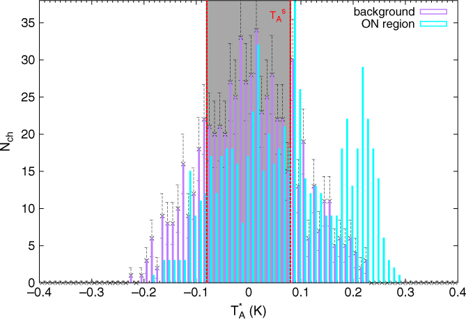
Figure A.2. Binned distribution of the number of channels $N_\mathrm{ch}\left(T_\mathrm{A}^{*}\right)$
as a function of the antenna temperature
$N_\mathrm{ch}\left(T_\mathrm{A}^{*}\right)$
as a function of the antenna temperature $T_\mathrm{A}^{*}$
. The purple histogram and error-bars represent the median and third-quartile background distribution, respectively, while the cyan histogram represents the distribution of the ‘ON’ region. The red dashed vertical lines highlight the threshold antenna temperature
$T_\mathrm{A}^{*}$
. The purple histogram and error-bars represent the median and third-quartile background distribution, respectively, while the cyan histogram represents the distribution of the ‘ON’ region. The red dashed vertical lines highlight the threshold antenna temperature $T_\mathrm{A}^{s}$
. Finally, the channels within the grey shaded area are rejected in our analysis.
$T_\mathrm{A}^{s}$
. Finally, the channels within the grey shaded area are rejected in our analysis.
Now that the integrated intensity maps are made, we need to establish the background level for each maps. Indeed, our new integrated intensity maps are not devoid of noise despite our aforementioned cuts. To do so, we simulate data consisting of noise with the same T rms as per our data-cubes. Using the same aforementioned steps, we produce integrated intensity maps within the same velocity ranges. We then define our noise level for our integrated intensity maps as the 99% distribution value of the ‘noise maps’ distribution.
A.2. Comparison of methods
Figure B.1 compares the CS(1–0) integrated intensity maps using uncleaned data-cubes with the standard intensity maps after removing baseline ripples, and with the method used in this work, to obtain integrated intensity maps. We remark the striking difference between the uncleaned and cleaned data. We finally notice the removal of additional noise using our method.
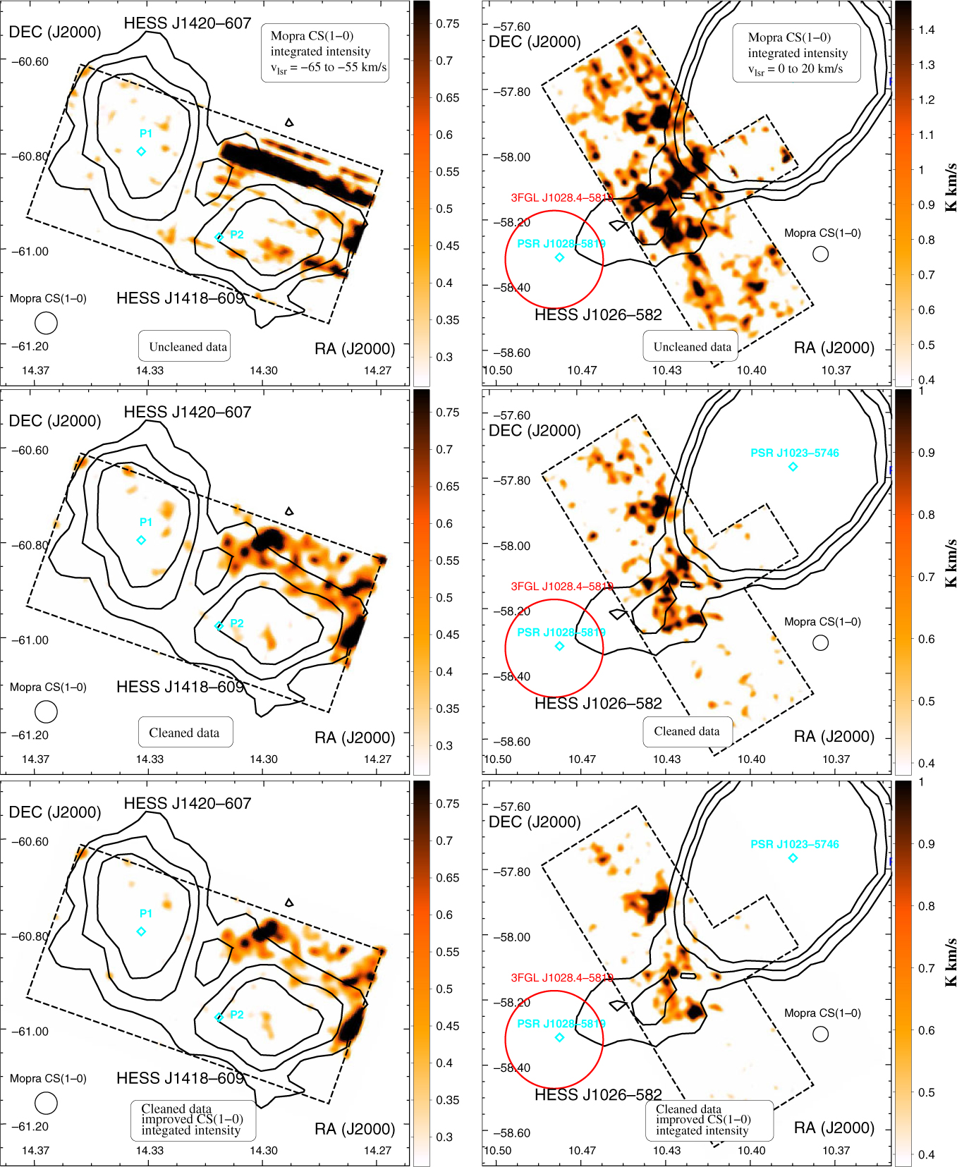
Figure A.3. Diagram indicating the position of the spiral arm in our Galaxy based on Vallée (Reference Vallée2013) model. The various lines with ticks represent the direction of the various TeV sources studied in this paper. For each TeV source, the brown, cyan, yellow, and brown regions indicate the distances of velocity ranges assumed for each source (see Figures 3, 4, 5, 7, 9, and 11)
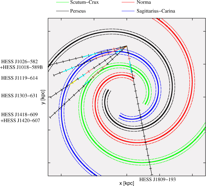
Figure B.1. Mopra CS(1–0) integrated intensity maps towards HESS J1418–609 and HESS J1420–607 (left panels) and HESS J1026–582 (right panels). Top panels illustrate the standard integrated intensity using uncleaned data-cubes. The middle panels highlight the CS(1–0) integrated intensity after removing baseline ripples (see Figure A.1). Finally, the bottom panels shows the final product from our method described in Appendix A.
Appendix B. Galactic model
We used the Galactic model from Vallée (Reference Vallée2013) (see Figure A.3) to help identify the Galactic arm in which each MC is located.
Appendix C. Fit parameters
Tables C.1–C.6 show the (RA, Dec) position, the semi-major axes and the Gaussian fitting parameters of the CS(1–0), C34S(1–0), HC3N(5–4, F = 4 − 3), SiO(1–0, v = 0), and CO(1–0) detections found towards the studied TeV sources.
Table C.1. Position, size, and fitting parameters of the emission traced by CS(1–0), its isotopologue C34S(1–0), CO(1–0), and HC3N(5–4, F = 4 − 3) towards HESS J1809–193. $T_{\mathrm{A}}^{*}$
denotes the peak temperature at v
lsr = v
cent, Δv indicates the full width at half maximum (FWHM) of a Gaussian fit, and W represents the main beam integrated intensity using a main beam efficiency factor η
mb (see Urquhart et al. Reference Urquhart2010 and text). Finally, the {indicates that the two components with little velocity separation are physically connected.
$T_{\mathrm{A}}^{*}$
denotes the peak temperature at v
lsr = v
cent, Δv indicates the full width at half maximum (FWHM) of a Gaussian fit, and W represents the main beam integrated intensity using a main beam efficiency factor η
mb (see Urquhart et al. Reference Urquhart2010 and text). Finally, the {indicates that the two components with little velocity separation are physically connected.
Table C.2. Position, size, and fitting parameters of the emission traced by CS(1–0) and CO(1–0) towards HESS J1026–582. $T_{\rm{A}}^*$
denotes the peak temperature at v
lsr = v
cent, Δv indicates the full width at half maximum (FWHM) of a Gaussian fit, and W represents the main beam integrated intensity using a main beam efficiency factor η
mb (see Urquhart et al. Reference Urquhart2010 for 7-mm tracers)). Finally, the {indicates that the two components with little velocity separation are physically connected.
$T_{\rm{A}}^*$
denotes the peak temperature at v
lsr = v
cent, Δv indicates the full width at half maximum (FWHM) of a Gaussian fit, and W represents the main beam integrated intensity using a main beam efficiency factor η
mb (see Urquhart et al. Reference Urquhart2010 for 7-mm tracers)). Finally, the {indicates that the two components with little velocity separation are physically connected.
Table C.3. Position, size, and fitting parameters of the emission traced by CO(1–0) towards HESS J1119–582. $T_{\mathrm{A}}^{*}$
denotes the peak temperature at v
lsr = v
cent, v indicates the full width at half maximum (FWHM) of a Gaussian fit, and W represents the main beam integrated intensity using the main beam efficiency factor η
mb (see Urquhart et al. Reference Urquhart2010 for 7-mm tracers). Finally, the {indicates that two the two components with little velocity separation are physically connected.
$T_{\mathrm{A}}^{*}$
denotes the peak temperature at v
lsr = v
cent, v indicates the full width at half maximum (FWHM) of a Gaussian fit, and W represents the main beam integrated intensity using the main beam efficiency factor η
mb (see Urquhart et al. Reference Urquhart2010 for 7-mm tracers). Finally, the {indicates that two the two components with little velocity separation are physically connected.
Table C.4. Position, size, and fitting parameters of the emission traced by CS(1–0) and CO(1–0) towards HESS J1418–609 and HESS J1420–607. $T_{\rm{A}}^*$
denotes the peak temperature at v
lsr = v
cent, Δv indicates the full width at half maximum (FWHM) of a Gaussian fit, and W represents the main beam integrated intensity using the main beam efficiency factor η
mb (see Urquhart et al. Reference Urquhart2010 for tracers). Finally, the {indicates that the two components with little velocity separation are physically connected.
$T_{\rm{A}}^*$
denotes the peak temperature at v
lsr = v
cent, Δv indicates the full width at half maximum (FWHM) of a Gaussian fit, and W represents the main beam integrated intensity using the main beam efficiency factor η
mb (see Urquhart et al. Reference Urquhart2010 for tracers). Finally, the {indicates that the two components with little velocity separation are physically connected.
Table C.5. Position, size, and fitting parameters of the emission traced by CS(1–0) and CO(1–0) transitions towards HESS J1303–631. $T_{\mathrm{A}}^{*}$
denotes the peak temperature at v
lsr = v
cent, Δv indicates the full width at half maximum (FWHM) of a Gaussian fit, and W represents the main beam integrated intensity using the main beam efficiency factor η
mb (see Urquhart et al. Reference Urquhart2010 for 7-mm tracers). Finally, the {indicates that two the two components with little velocity separation are physically connected.
$T_{\mathrm{A}}^{*}$
denotes the peak temperature at v
lsr = v
cent, Δv indicates the full width at half maximum (FWHM) of a Gaussian fit, and W represents the main beam integrated intensity using the main beam efficiency factor η
mb (see Urquhart et al. Reference Urquhart2010 for 7-mm tracers). Finally, the {indicates that two the two components with little velocity separation are physically connected.

Table C.6. Position, size, and fitting parameters of the emission traced by CO(1–0) towards HESS J1018–589B. $T_{\mathrm{A}}^{*}$
denotes the peak temperature at v
lsr = v
cent, Δv indicates the full width at half maximum (FWHM) of a Gaussian fit, and W represents the main beam integrated intensity using a main beam efficiency factor η
mb (see Urquhart et al. Reference Urquhart2010 for 7-mm tracers).
$T_{\mathrm{A}}^{*}$
denotes the peak temperature at v
lsr = v
cent, Δv indicates the full width at half maximum (FWHM) of a Gaussian fit, and W represents the main beam integrated intensity using a main beam efficiency factor η
mb (see Urquhart et al. Reference Urquhart2010 for 7-mm tracers).

Appendix D. Physical parameters
D.1. CS(1–0)
The averaged optical depth τ
CS(1–0) can be derived using the integrated intensity ratio W
CS(1–0) and $W_{\textrm{C}^{34}\textrm{S(1--0)}}$
as follows:
$W_{\textrm{C}^{34}\textrm{S(1--0)}}$
as follows:
 $$\begin{equation}\label{tauCS}\frac{W_{CS(1-0)}}{W_{C^{34}S(1-0)}} = \frac{1-e^{-\tau_{CS(1-0)}}}{1-e^{\alpha\tau_{CS(1-0)}}}\end{equation}
where α = [32S]/[34S] = 22 represents the abundance ratio between the two isotopologues based on terrestrial measurements (Fink Reference Fink1981). We obtain the column density of the upper state $N_{\textrm{CS}_1}$
:
$N_{\textrm{CS}_1}$
:
 $$\begin{equation}\label{CSeq2} N_{\textrm{CS}_1} = \frac{8k \pi\nu_{10}^{2}}{A_{10}hc^{3}}\left(\frac{\Delta\Omega_{\textrm{A}}}{\Delta\Omega_{\textrm{S}}}\right)\left(\frac{\tau_{\textrm{CS(1-0)}}}{1-e^{-\tau_{\textrm{CS(1-0)}}}}\right)\int{T_{\textrm{mb}}\left(v\right)dv}\vspace*{-12pt}\end{equation}
Assuming the gas to be in local thermal equilibrium at temperature T kin, we can thus obtain the total CS column density N CS:
 $$\begin{equation} \label{CSeq3} N_{CS} = N_{CS_1}\left(1+\frac{1}{3}e^{2.35/T_{\textrm{kin}}}+\frac{5}{3}e^{-4.7/T_{\textrm{kin}}}+\textrm{...}\right)\end{equation}
D.2. Mass and density
 $$ \begin{equation}M_{\textrm{H}_2}=\mu m_{\textrm{H}}\pi abN_{\textrm{H}_2}\end{equation}
with μ = 2.8 being the averaged atomic weight (accounting for 20% Helium), mH the hydrogen mass and a,b the semi-minor and semi-major axis of the selected elliptic regions.
 $$\begin{equation} n_{\textrm{H}_2}=\frac{M}{4/3\left(\mu m_{\textrm{H}}\right)\pi ab^2} \end{equation}
D.3. Physical parameters of individual sources
Tables D.1–D.6 show the column density $N_{\textrm{H}_2}$
the atomic and molecular mass
$N_{\textrm{H}_2}$
the atomic and molecular mass $M_{\textrm{H}_\textsc{i}}$
and
$M_{\textrm{H}_\textsc{i}}$
and $M_{\textrm{H}_2}$
, and molecular density
$M_{\textrm{H}_2}$
, and molecular density $n_{\textrm{H}_2}$
estimates based on the CS, CO, and H
i
emission found towards the regions listed in Appendix C.
$n_{\textrm{H}_2}$
estimates based on the CS, CO, and H
i
emission found towards the regions listed in Appendix C.
Table D.1. Physical parameters obtained from our CS and CO analyses for the different selected regions located towards HESS J1809–193. In the case where C34S(1–0) is detected, the derived optical depth τ
CS(1–0) is shown as superscript next to the CS column density N
CS. Otherwise, an optical thin scenario is assumed and the derived column densities $N_{\mathrm{H}_2}$
and N
CS, mass
$N_{\mathrm{H}_2}$
and N
CS, mass $M_{\mathrm{H}_2} \ (CS)$
, and H2 averaged density
$M_{\mathrm{H}_2} \ (CS)$
, and H2 averaged density $n_{\mathrm{H}_2} \ (CS)$
act as lower limits.
$n_{\mathrm{H}_2} \ (CS)$
act as lower limits.
Table D.2. Physical parameters obtained from our CS and CO analyses for the different selected regions located towards HESS J1026–582. In the case of our CS analysis, we assumed a optically thin scenario and the derived column densities $N_{\mathrm{H}_2}$
and N
CS, mass
$N_{\mathrm{H}_2}$
and N
CS, mass $M_{\mathrm{H}_2} \ (CS)$
, and H2 averaged density
$M_{\mathrm{H}_2} \ (CS)$
, and H2 averaged density $n_{\mathrm{H}_2} \ (CS)$
act as lower limits.
$n_{\mathrm{H}_2} \ (CS)$
act as lower limits.
Table D.3. Physical parameters obtained from our CO analysis for the different selected regions located towards HESS J1119–582.
Table D.4. Physical parameters obtained from our CS and CO analyses for the different selected regions located towards HESS J1303–631. In the case of our CS analysis, we assumed a optically thin scenario and the derived column densities $N_{\mathrm{H}_2}$
and N
CS, mass
$N_{\mathrm{H}_2}$
and N
CS, mass $M_{\mathrm{H}_2} \ (CS)$
, and H2 averaged density
$M_{\mathrm{H}_2} \ (CS)$
, and H2 averaged density $n_{\mathrm{H}_2} \ (CS)$
act as lower limits.
$n_{\mathrm{H}_2} \ (CS)$
act as lower limits.
Table D.5. Physical parameters obtained from our CS and CO analyses for the different selected regions located towards HESS J1420–607 and HESS J1418–609. In the case of our CS analysis, we assumed a optically thin scenario and the derived column densities $N_{\mathrm{H}_2}$
and N
CS, mass
$N_{\mathrm{H}_2}$
and N
CS, mass $M_{\mathrm{H}_2} \ (CS)$
, and H2 averaged density
$M_{\mathrm{H}_2} \ (CS)$
, and H2 averaged density $n_{\mathrm{H}_2} \ (CS)$
act as lower limits.
$n_{\mathrm{H}_2} \ (CS)$
act as lower limits.
Table D.6. Physical parameters obtained from our CO analysis for the different selected regions located towards HESS J1018–589B.
Appendix E. Column densities and distance studies
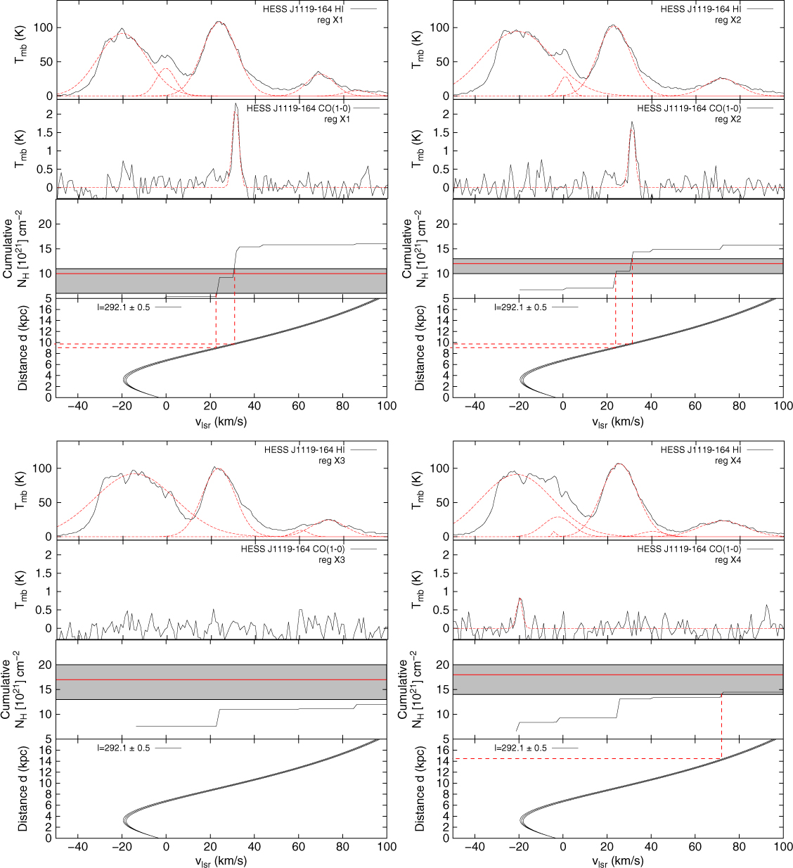
Figure E.1. Averaged SGPS (first panels) and Nanten CO(1–0) emission (second panels) towards the region ‘A’ (left) and the western part of the SNR (right) (see Figure 5). The different Gaussian fits are shown as red dashed lines. At each Gaussian peak, the Hi and CO(1–0) emission have been integrated and converted into column density, N H (third panel), via the X CO and the X HI factors (see text). Here, all emission are assumed to be in the far distance. The grey regions show the X-ray absorbed column density range obtained by Pivovaroff et al. (Reference Pivovaroff, Kaspi, Camilo, Gaensler and Crawford2001). The fourth panels indicate the Galactic rotation curve towards the position (RA, Dec) = (291.1 ± 0.5, −0.3) with the red dashed lines delimiting the distance where our column densities match with the X-ray column densities while the blue dashed line indicates the distance where the column density in the western region roughly equals the column density in the eastern region.
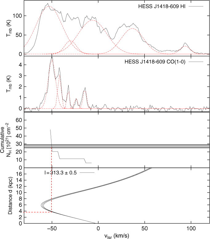
Figure E.2. Averaged SGPS Hi and Nanten CO(1–0) emission towards HESS J1418–609 (see Fig. 6) in black solid lines. In both panels, the Gaussian fits are shown as red dashed lines. At each Gaussian peak, the Hi and CO(1–0) emission have been integrated and converted into N H column density via the X CO and X HI, respectively (see text). The bottom panel indicates the evolution of the distance towards the position (313 ± 0.5, 0.1) as a function of kinematic velocity.
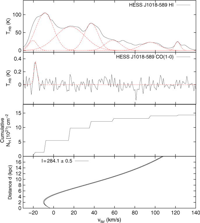
Figure E.3. Averaged GASS Hi and Nanten CO(1–0) emission towards HESS J1018–589 (see Fig. 11) in black solid lines. In both panels, the Gaussian fits are shown as red dashed lines. At each Gaussian peak, the Hi and CO(1–0) emission have been integrated and converted into N H cumulative column density via the X CO and X HI, respectively (see text). The bottom panel indicates the kinematic distance towards the position (RA, Dec) = (284 ± 0.5, −1.7) as a function of kinematic velocity v lsr.
Appendix F. HESS J1809–193 additional figures
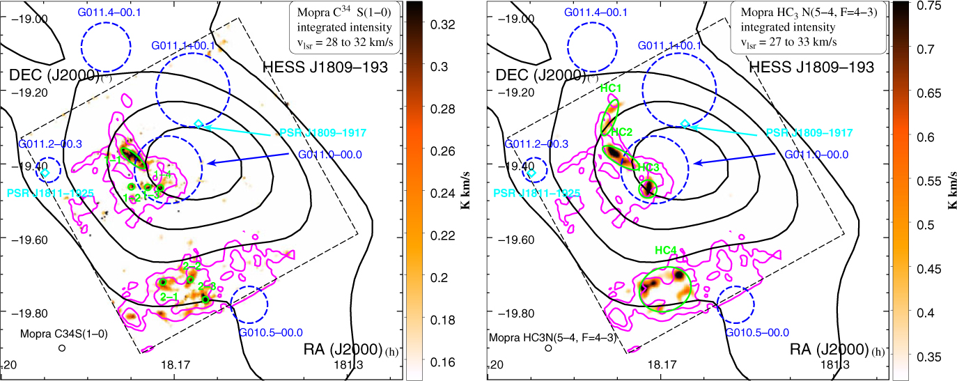
Figure F.1. Mopra C34S(1–0) (left panel) and HC3N(5–4, F = 4 − −3) (right panel) integrated intensity between v lsr = 28 to 32 km/s and v lsr = 27 to 32 km/s, respectively, towards HESS J1809–193. The various C34S detections labelled ‘1–1 to 1–4’ and ‘2–1 to 2–3’ (left panel) and the HC3N detections labelled ‘HC1 to HC4’ are shown in green ellipses. In both panels, the CS(1–0) integrated intensity between v lsr = 25 to 38 km/s are shown in purple. The SNRs are shown as dashed blue circles while the position of the pulsars PSR J1809–1917 and PSR J1811–1925.


