2. Experiments and data processing

The Qingtu Lake observation array (QLOA), for studies on high-Reynolds-number canonical TBL layers as well as sand-laden two-phase flows, has been built in Minqin, China, and observational data have been accumulated in recent years. The array contains 1 main 32 m tower and 23 5 m towers set in the Cartesian coordinate system. Eleven sonic anemometers (CSAT3B, Campbell Scientific) with sampling frequency 50 Hz are equipped logarithmically on the main tower from $z = 0.9$ to 30 m to measure the three components of wind velocities ($u$, $v$ and $w$ in the streamwise, spanwise and wall-normal directions, respectively) and the temperature. Moreover, based on the light scattering method (Shaughnessy & Morton Reference Shaughnessy and Morton1977), eleven aerosol monitors (DUSTTRAK II-8530-EP, TSI Incorporated) with sampling frequency 1 Hz were installed on the main tower at the same height as the sonic anemometers to collect the concentration information of PM10 (particles with sizes smaller than $10\,\mathrm {\mu }$m). A panorama view of the QLOA, a schematic diagram of the installation of various probes, and additional details on the experimental set-up can be found in Liu, He & Zheng (Reference Liu, He and Zheng2023).

Limited by the complex and uncontrollable nature of the ASL, not all the data are suitable for the study of wall turbulence. Therefore, rigorous data pre-processing is required to select suitable turbulence data. Following standard practice in the analysis of ASL data (Wyngaard Reference Wyngaard1992), the synchronously raw measured data are divided into multiple hourly time series to ensure statistical convergence (also confirmed by Ogive analysis) of the data and the corresponding spectra for subsequent processing (Hutchins et al. Reference Hutchins, Chauhan, Marusic, Monty and Klewicki2012). The data processing methods include wind direction correction (Wilczak, Oncley & Stage Reference Wilczak, Oncley and Stage2001), steady wind selection (Foken et al. Reference Foken, Gockede, Mauder, Mahrt, Amiro and Munger2004), thermal stratification stability judgement (Stull Reference Stull1988) and detrending manipulation (Hutchins et al. Reference Hutchins, Chauhan, Marusic, Monty and Klewicki2012). The detailed procedure can be found in Liu et al. (Reference Liu, He and Zheng2023). The corresponding fluctuating signal can be obtained by subtracting the 1 h mean value of the signal after rigorous data pre-processing. The particle-free and particle-laden experimental datasets (fluctuating velocity and corresponding fluctuating PM10 concentration) employed herein were recorded by Wang & Zheng (Reference Wang and Zheng2016) and Liu et al. (Reference Liu, He and Zheng2023), respectively. The validation and comparison of the selected data under particle-free and particle-laden conditions are shown in Liu, He & Zheng (Reference Liu, He and Zheng2021) and Liu et al. (Reference Liu, He and Zheng2023) by checking the basic statistics. The particle characteristics parameters (e.g. particle density, response time, Froude number and Stokes number) are listed in table 1, and the detailed calculation procedures of turbulent velocity and particle information can be found in Liu et al. (Reference Liu, He and Zheng2023). Moreover, as the particle size distribution shown in Liu et al. (Reference Liu, He and Zheng2023) indicates, there are still larger particles (${>}10\,\mathrm {\mu }$m) in particle-laden flows. Due to the constraints of the environment and instruments, it is not feasible to measure effectively the temporal variations of larger particles. In this study, the dust (${<}10\,\mathrm {\mu }$m) concentration is considered as the main research object to study their structure characteristics. The flow fields with mean dust concentrations ${<}0.1$ and >0.1 mg m$^{-3}$ are considered to be particle-free and particle-laden flows, respectively. The variation of dust concentration collected in the corresponding particle-laden flow field is known as the dust concentration field.

Table 1. Basic parameters of fluid and particles in the ASL: $\sigma$ is the root mean square of the streamwise velocity fluctuation, $\kappa = 0.41$ is the Kármán constant, $\nu$ is the kinetic viscosity that is estimated based on the pressure and temperature of the site (Tracy, Welch & Porter Reference Tracy, Welch and Porter1980), $U_{\tau }$ is the friction velocity, which is estimated as $\sqrt {-\overline {uw}}$ at $z = 2.5$ m following Hutchins et al. (Reference Hutchins, Chauhan, Marusic, Monty and Klewicki2012) and Li & McKenna Neuman (Reference Li and McKenna Neuman2012), $\delta$ is the boundary layer thickness collected by Doppler LiDAR (Liu et al. Reference Liu, He and Zheng2023), $\bar {u}$ is the local mean velocity, $R_{uu}(\tau )$ and $T_{0}$ are the temporal autocorrelation function and the corresponding first zero-crossing point (Emes et al. Reference Emes, Arjomandi, Kelso and Ghanadi2019; Li et al. Reference Li, Lim, Berk, Abraham, Heisel, Guala, Coletti and Hong2021), and $C$ and $P_{d}$ are the mean concentration and percentage of PM10.

As reported previously (Baars et al. Reference Baars, Hutchins and Marusic2017; Krug et al. Reference Krug, Baars, Hutchins and Marusic2019; Baars & Marusic Reference Baars and Marusic2020a), the LCS method employed in this study is effective in extracting wall-attached structures. However, there is no doubt that this method does not exclusively decompose wall-attached self-similar structures: not only wall-attached self-similar structures, but also wall-attached non-self-similar structures are contained (Marusic & Monty Reference Marusic and Monty2019; Yoon et al. Reference Yoon, Hwang, Yang and Sung2020). Deshpande et al. (Reference Deshpande, Chandran, Monty and Marusic2020) and Deshpande, Monty & Marusic (Reference Deshpande, Monty and Marusic2021) noted this limitation and described methods (two-dimensional cross-spectrum) to differentiate them. However, due to the limitations of the observation environment, it is difficult to obtain a two-dimensional energy spectrum of the signal under current experimental conditions. So in the current study, no strict distinction is made between wall-attached self-similar structures and wall-attached non-self-similar structures (even though the self-similarity is obvious).

3. Characteristics of the wall-attached structures

To investigate the characteristics of the wall-attached structures, the coherence in different scales based on the LCS are explored first. The coherence spectrogram for the particle-free data with the lowest reference point $z_{R}/\delta = 0.006$ from the QLOA is shown in figure 2(a). The coherence spectrograms are reflected by increasing greyscales. It can be noted that there exists a region in the $(\lambda _{x}, z)$ space where $\gamma ^{2}$ is the isocontour alignment with lines of constant $\lambda _{x}/\Delta z$ (with $\Delta z$ the wall-normal separation to the lowest observation point). In addition, consistent with the results obtained from canonical TBL experiments, with the superposition of hierarchical structures in the flow field, the magnitude of the coherence spectrum in large-scale ranges near the wall is most significant; i.e. increasing coherence accumulates in large-scale components near the wall (Baars et al. Reference Baars, Hutchins and Marusic2017; Duan et al. Reference Duan, Zhang, Zhong, Zhu and Li2020). In the logarithmic layer, the magnitude of $\gamma ^{2}$ increases linearly with $\log (\lambda _{x})$ for a constant $\Delta z$ (which is more intuitive in figure 2d), which is the nature of a geometrically self-similar structure (Baars et al. Reference Baars, Hutchins and Marusic2017; Krug et al. Reference Krug, Baars, Hutchins and Marusic2019). The results indicate that the data collected in the QLOA can effectively capture wall-attached structures through the LCS, similar to the results of laboratory experiments and ASL observations from the SLTEST under near-neutral conditions. Notably, in wall turbulence studies, the lower the reference position ($z_{R} \rightarrow 0$), the greater the amount of wall-attached hierarchical organization of eddies that can be captured. However, because of the limitations of field observation conditions, it is difficult to reach the extreme near-wall position as in laboratory experiments. Therefore, with reference to the available field observations, $z/\delta = 0.006$ is taken as the reference height in this study, which is lower than the reference position in Krug et al. (Reference Krug, Baars, Hutchins and Marusic2019). The implied geometrical self-similarity is obviously equivalent to the attached eddy framework discussed above if $\Delta z \approx z$, which is approached either for $z_{R} \rightarrow 0$ or for $z \gg z_{R}$ in experiments. For a large $\Delta z$, there is no difference between plotting $\gamma ^2$ as a function of $z$ or $\Delta z$, consistent with the expectation at $\Delta z \gg z_{R}$ (Krug et al. Reference Krug, Baars, Hutchins and Marusic2019). Therefore, in the subsequent study, normalization with $\Delta z$ is used, as this approach provides a more extensive scaling region. In addition, similar special regions are observed in the particle-laden flow fields (figure 2b) and dust concentration fields (figure 2c) (the variables $u$ in (1.2) are replaced by the dust concentration fluctuations $c$ at the corresponding height). This means that under the influence of particles, wall-attached structures still exist in the particle-laden flow field; moreover, some special particle clustering structures occur in the concentration field.

Figure 2. Coherence spectrograms of streamwise velocity fluctuations $u$ in (a) particle-free, (b) particle-laden and (c) dust concentration fluctuations $c$. (d,e,f) The corresponding three-dimensional coherence spectrograms with the wavelength axis predivided by $\Delta z$.

When the streamwise wavelength is scaled by the local height $\Delta z$, the LCS of the dust concentration fluctuation $c$ (figure 2f) obtained synchronously with the streamwise velocity fluctuation $u$ from QLOA shows a signature similar to the LCS of $u$ under particle-free/laden conditions (figures 2d,e) and that in laboratory experiments (Baars et al. Reference Baars, Hutchins and Marusic2017; Baidya et al. Reference Baidya2019). The spectral characteristic of the dust concentration fluctuation $c$ may be analogous to that of the streamwise velocity fluctuation $u$, i.e. there exists a certain region in $(\lambda _{x},\Delta z)$ space (shown by the grey inclined plane) where the LCS lines at different heights follow the same increasing pattern with increasing wavelength. The region adheres to

(3.1)\begin{equation} \gamma^{2} = C_{1} \ln (\lambda_{x}/\Delta z) + C_{2}, \end{equation}

where $C_{1}$ and $C_{2}$ are constants, and the region is consistent with the inclined plane recorded in Baars et al. (Reference Baars, Hutchins and Marusic2017). These signatures are reminiscent of the hierarchy of attached eddies in streamwise velocity fluctuations (Baars et al. Reference Baars, Hutchins and Marusic2016). This indicates that there are wall-attached dust clustering structures with self-similar nature in the dust concentration field, whose characteristics and differences from those of $u$ need to be clarified further.

After describing the qualitative characteristics of the LCS of $u$ in the flow fields (under particle-free and particle-laden conditions) and those of $c$ in dust concentration fields, the variation in the coherent characteristics with the wall-normal position of the reference point is further investigated. The LCS plots for flow fields under particle-free and particle-laden conditions and for dust concentrations with reference points at $z_{R}/\delta = 0.006$, 0.0167, 0.0333 and 0.0567 are shown in figures 3(a), 3(b) and 3(c), respectively. As the height of the reference point spans one order of magnitude, the coherence characteristics of both the flow fields and the dust concentration field change significantly. When the reference point is close to the wall ($z_{R}/\delta = 0.006$), the captured spectra exhibit good collapse, which is consistent with the result from TBLs in Baars et al. (Reference Baars, Hutchins and Marusic2017). This means that the coherent structures captured by the reference point closest to the wall exhibit obvious self-similarity, as described by the classic AEH (the size of the eddy is proportional to its distance from the wall) (Townsend Reference Townsend1976), which can further be used to investigate the scale and energy characteristics of wall-attached structures. In addition, when the traversing points become higher while the reference point is invariant (the red arrow in figure 3), the spectral lines gradually decrease. This is because with increasing height of the traversing point, the captured hierarchies of eddies attached to the wall decrease, and only larger hierarchies can be captured, leading to a lower coherence $\gamma ^{2}$.

Figure 3. Obtained LCS plots with different reference height $z_{R}$: (a) results for $u$ in the particle-free flow, (b) results for $u$ in particle-laden flow, and (c) the corresponding LCS plots for dust concentration fluctuation $c$. The grey lines are from fitting (3.1). The grey dashed lines are copies of the fitting lines in the leftmost plots.

On the basis of the qualitative variations in the LCS characteristics, the respective LCS plots for different phases (flow field and dust concentration field) in high-Reynolds-number ASLs are further investigated under different conditions. The leftmost plots in figures 3(a) and 3(b) show the $\Delta z$-scaled LCS plots for streamwise velocity fluctuations $u$ in particle-free and particle-laden flows, respectively. The leftmost plot in figure 3(c) shows the $\Delta z$-scaled LCS for dust concentration $c$. Notably, all the LCS plots collapse well within a certain wavelength range, which agrees with the results of existing laboratory particle-free TBL experiments (Baars et al. Reference Baars, Hutchins and Marusic2017; Baars & Marusic Reference Baars and Marusic2020a). As discussed in § 2, due to the limitation of the LCS, the wall-attached non-self-similar structures are not completely excluded. However, the present results still exhibit an obvious self-similar nature due to the high-Reynolds-number condition. A high Reynolds number ensures adequate scale separation, which likely results in the inclusion of many structures scaled by $z$ (i.e. self-similar). This means that the energetic wall-attached eddies are predominantly self-similar. Moreover, the spectral characteristic of the dust concentration fluctuation $c$ may be analogous to that of the streamwise velocity fluctuation $u$. There exists a self-similar region in the spectral space where the LCS lines in the flow and those in the dust concentration field satisfy (3.1). The fitting parameters $(C_{1}, C_{2})$ for streamwise velocity fluctuations under particle-free and particle-laden conditions and for dust concentration are $(0.367 \pm 0.009, -0.97 \pm 0.03)$, $(0.360 \pm 0.002, -0.919 \pm 0.007)$ and $(0.348 \pm 0.003, -0.864 \pm 0.011)$, respectively. Moreover, the minimum streamwise wavelength at which the energetic variance still appears relative to its wall-normal extent is called the aspect ratio ($AR$) (Baars et al. Reference Baars, Hutchins and Marusic2017), i.e.

(3.2)\begin{align} AR & = \left.\frac{\lambda_{x}}{z}\right|_{\gamma^{2}=0} \approx \left.\frac{\lambda_{x}}{\Delta z}\right|_{\gamma^{2}=0} \nonumber\\ & = \exp\left(-\frac{C_{2}}{C_{1}}\right). \end{align}

Following the aforementioned approximation, $\lambda _{x}/\Delta z$ is approximately equal to $\lambda _{x}/z$. The aspect ratios for streamwise velocity fluctuations $u$ under particle-free and particle-laden conditions and for dust concentration $c$ can be obtained based on the definition of the aspect ratio. The results are listed in table 2, and the previously documented laboratory experimental results have also been added for comparison. Based on error propagation (Hughes & Hase Reference Hughes and Hase2010), the errors of $AR$ are calculated and added in table 2. The aspect ratio in this study for wall-attached self-similar structures in particle-free flow ($AR_{uf} = 14.1 \pm 1.5$) agrees with the particle-free TBL ($AR = 14$; Baars et al. Reference Baars, Hutchins and Marusic2017), channel ($AR = 13.9$; Duan et al. Reference Duan, Zhang, Zhong, Zhu and Li2020) and other ASL ($AR = 14$; Krug et al. Reference Krug, Baars, Hutchins and Marusic2019) results, which further validates the reasonability of the reference height used here and the correctness of the results. This reference height can be used to extract wall-attached structures. Based on the same process, the aspect ratios in particle-laden conditions, for wall-attached velocity and concentration structures, are $AR_{ul} = 12.8 \pm 0.3$ and $AR_{c} = 12.0 \pm 0.5$, respectively. It is worth noting that the aspect ratio for dust concentration is comparable to that for temperature fluctuation ($AR_{\theta } \approx 10.6$; Krug et al. Reference Krug, Baars, Hutchins and Marusic2019), which is also taken as scalar, and presumably would be equivalent to particles in the low $St$ limit. In addition, the results in this study indicate that although the aspect ratios of the wall-attached structures in particle-laden flow and in the dust concentration field are smaller than that in particle-free flow field from the perspective of mean value, this difference is not significant enough under the present conditions when taking provided error ranges into account. However, this decreasing tendency is to be anticipated by the close connection between the aspect ratio and the structure inclination angle. According to the definition of the structure inclination angle (Marusic & Heuer Reference Marusic and Heuer2007; Liu, Bo & Liang Reference Liu, Bo and Liang2017), the larger the structure inclination angle, the smaller the aspect ratio. Tay, Kuhn & Tachie (Reference Tay, Kuhn and Tachie2015) and Wang, Gu & Zheng (Reference Wang, Gu and Zheng2020) found that the addition of a large number of particles into a particle-laden flow leads to an increase of the inclination angle in the horizontal channel and ASL, respectively. Besides, the variation in the structure inclination angle can be attributed to the ‘stretching’ effect of the velocity gradient (Adrian, Meinhart & Tomkins Reference Adrian, Meinhart and Tomkins2000; Dennis Reference Dennis2015), and previous research has suggested that particles lead to a reduction in the velocity gradient and thus increase the structure inclination angle (Wang et al. Reference Wang, Gu and Zheng2020); the aspect ratio is then expected to be reduced.

Table 2. Aspect ratios obtained by the LCS for different flow types.

When the reference point becomes higher (the orange arrow in figure 3), the LCS collapsing characteristics (scaling trends) for both fluctuating velocity (figures 3a,b) and dust fluctuating concentration (figure 3c) are no longer obvious until they disappear ($z_{R}/\delta = 0.0567$). For further comparison, the fitting lines for $z_{R}/\delta = 0.006$ are re-plotted to the LCS at each higher reference point, indicated by the grey dashed lines. It can be seen that with the decreasing of the traversing point positions, the corresponding LCS plots become much greater than the expected scaling trends, and the corresponding ratio threshold ($\lambda _{x}/\Delta z|_{\gamma ^{2}=0}$) decreases. This means that with increasing reference height, the coherent structures captured by the LCS plots not only include the part attached to the wall but also contain large-scale energetic structures that are not attached to the wall (Baars & Marusic Reference Baars and Marusic2020a; Hu et al. Reference Hu, Yang and Zheng2020). A similar result also appears in laboratory TBLs, but this phenomenon is not as significant as that in ASLs due to the limitation of the Reynolds number (figure 10 in Baars & Marusic Reference Baars and Marusic2020a). This suggests that the non-attached eddies mask the self-similar characteristics of the wall-attached eddies exhibiting the failure of the scaling collapse. As mentioned above, theoretically, the closer the reference position is to the wall, the closer the result is to the AEH. However, limited by the field observation conditions, the lowest observational reference point $z_{R}/\delta = 0.006$ ($z_{R}^+ \equiv z_{R}U_{\tau }/\nu \sim O(10^{4})$) is adopted in this study. This value is much lower than the reference point ($z_{R}/\delta = 0.0233$) in Krug et al. (Reference Krug, Baars, Hutchins and Marusic2019), which also used field data to estimate the flow field coherence through LCS plots. In this situation, $\Delta z \approx z$, the self-similarity for the flow field and that for the dust concentration field are investigated.

4. Spectral scaling of fluctuating streamwise velocity and dust concentration

Self-similar structure characteristics of fluctuating streamwise velocity and dust concentration have been identified, and their aspect ratios have been assessed from the coherence between the turbulence signals at the traversing points and at the near-wall reference point in the flow and dust concentration fields in § 3. On this basis, much attention should be given to the energy, and it is necessary to further investigate the energy spectra of this type of wall-attached structure. To obtain the energy distribution characteristics of these wall-attached eddies in the flow field, spectral linear stochastic estimation (LSE), a data-driven decomposition method, is used to identify attached structures (Adrian Reference Adrian1979; Baars et al. Reference Baars, Hutchins and Marusic2016; Baars & Marusic Reference Baars and Marusic2020a,Reference Baars and Marusicb). The streamwise velocity fluctuations at the near-wall reference point and at the target point are $u(z_{R})$ and $u(z)$, respectively, and the coherent velocity $u_{A}(z)$ with respect to the reference point (approximately wall-attached) at the target point can be expressed as

(4.1)\begin{equation} \hat{u}_{A}(z;\lambda_{x}) = H(z,z_{R};\lambda_{x})\,\hat{u}(z_{R};\lambda_{x}), \end{equation}

where $H(z,z_{R};\lambda _{x})$ is the linear transfer kernel computed from

(4.2)\begin{align} H(z,z_{R};\lambda_{x}) &= \frac{\langle \hat{u}(z;\lambda_{x})\,\hat{u}^{*}(z_{R}; \lambda_{x})\rangle}{\langle \hat{u}(z_{R};\lambda_{x})\,\hat{u}^{*}(z_{R};\lambda_{x})\rangle} \nonumber\\ &= \frac{\varPhi_{uu}(z,z_{R};\lambda_{x})}{\varPhi_{uu}(z_{R};\lambda_{x})} \nonumber\\ &= \lvert H(z,z_{R};\lambda_{x})\rvert \exp({j\varphi(z,z_{R};\lambda_{x})}), \end{align}

comprising a wavelength-dependent linear gain $\lvert H\rvert$ and phase $\varphi$. Notably, the coherent velocity $\hat {u}_{A}(z;\lambda _{x})$ is not the imprint velocity of the reference velocity for one particular hierarchy eddy, but imprints from other hierarchies of eddies with heights exceeding $z$ (Hu et al. Reference Hu, Yang and Zheng2020). For this reason, the contribution of wall-attached structures to the streamwise turbulence intensity at different heights can be extracted. Furthermore, combining (1.2), (4.1) and (4.2), the coherent energy spectra with the near-wall position at the target point can be expressed as

(4.3)\begin{align} \varPhi_{uu}^{A}(z;\lambda_{x}) &= \lvert H(z,z_{R};\lambda_{x})\rvert^{2}\,\varPhi_{uu}(z_{R};\lambda_{x}) \nonumber\\ &= \gamma^{2}\,\varPhi_{uu}(z;\lambda_{x}). \end{align}

It can be noticed easily that the kernel for the LSE to detect these structures can be found via the LCS. The energy that is coherent with the wall is part of the total energy. The coherent portion $\varPhi _{uu}^{A}$ can be reconstructed via an LSE procedure and is equal to the energy spectra $\varPhi _{uu}$ at $z$ multiplied by $\gamma ^{2}$. As a data-driven scale-dependent filter, $\gamma ^{2}$ has the ability to decompose $\varPhi _{uu}$ or $\varPhi _{cc}$ into coherent and incoherent portions relative to $z_{R}$, following

(4.4)\begin{align} \underbrace{\varPhi_{uu}^{N}(z;\lambda_{x})}_{Wall\text{-}incoherent} & = \underbrace{\varPhi_{uu}(z;\lambda_{x})}_{Entire\ energy} - \underbrace{\gamma^{2}\,\varPhi_{uu}(z;\lambda_{x})}_{Wall\text{-}coherent} \nonumber\\ &= (1 - \gamma^{2})\,\varPhi_{uu}(z;\lambda_{x}). \end{align}

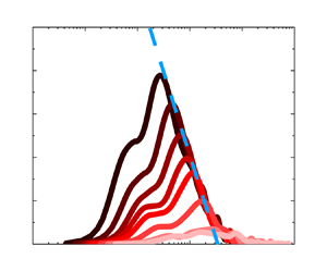
As derived above, the LCS provides information on how much energy is stochastically coherent/incoherent between $z$ and $z_{R}$. In this scenario, take dust concentration ($St_{\eta }\equiv \tau _{p}/\tau _{f}\sim O(10^{-2})$) as an example for illustration. The unfiltered premultiplied spectrum of the dust concentration at $z/\delta = 0.0567$ is shown in figure 4(a). The usual reason for premultiplying the spectrum by the wavenumber is to create a logarithmic plot in which equal areas under the curve correspond to equal energies (or variances) (Smits et al. Reference Smits, McKeon and Marusic2011). Notably, in the form of a premultiplied energy spectrum, the fluctuation intensity of multi-scale dust concentration lies mainly in $O(10^{0}) < k_{x}\delta < O(10^{1})$, and the corresponding wavelengths are approximately $0.6\delta\hbox{--}6\delta$. Figure 4(b) shows the LCS plots between the target point $z/\delta$ = 0.0567 and the near-wall reference point $z/\delta = 0.006$. When outer-scaling is adopted, the LCS reveals that the correlation with the near-wall signal is obvious when the wavenumber is less than 10, while it appears to level off as the wavenumber is less than 1 (Baars et al. Reference Baars, Hutchins and Marusic2017; Baars & Marusic Reference Baars and Marusic2020a). On this basis, the LCS is used here as a scale-dependent filter to decompose $\varPhi _{cc}(z;\lambda _{x})$ into stochastically wall-coherent and wall-incoherent portions, as shown in (4.4); the corresponding results are shown in figure 4(c). The black and yellow curves are the unfiltered premultiplied spectrum of the dust concentration and the corresponding LCS, respectively. The red and blue curves are the filtered wall-attached and non-attached portions, respectively. The energy peak from the premultiplied spectra of $c$ contains energies from both wall-attached and non-attached structures. Furthermore, non-attached dust clustering structures are located mainly in the small-scale range, while wall-attached clusters are the dominant structures in the large-scale range. This is anticipated because the smallest coherent motion that can be obtained from the coherence spectrum between two positions amounts to the separation distance; the length scale of the wall-attached structure is larger and the wall-attached structure can be detected more easily, while the smaller scales (the physical height is less than the separation distance) show no coherence.

Figure 4. Diagrams of the decomposition of the $c$ spectrum at location $z/\delta = 0.0567$: (a) the original energy spectrum, (b) the corresponding LCS, and (c) the decomposition results for wall-coherent (attached) component (red line) and wall-incoherent (non-attached) component (blue line) of the energy spectrum, via $\gamma ^{2}$ filter.

After performing the aforementioned data-driven decomposition (4.4) for all the energy spectra of the streamwise velocity fluctuations $u$ (in particle-free and particle-laden flows), throughout the entire observation range, the wall-attached and non-attached portions of the energy spectra can be obtained. The energy spectra of the fluctuating streamwise velocity under particle-free and particle-laden conditions with wall-scaling and outer-scaling are plotted in figures 5(a–c) and 5(d–f), respectively. The unfiltered outer-scaled energy spectra of $u$ are shown in figures 5(a,d), and wall-attached spectra with an wall-scaling are shown in figures 5(b,e) –and with an outer-scaling in figures 5(c,f). Figures 5(a) and 5(d) show that, regardless of whether the flow is particle-free or particle-laden, the unfiltered energy spectra exhibit a distinct peak that corresponds to the VLSMs in high-Reynolds-number wall-bounded flows, and an obvious pivoting phenomenon, i.e. the premultiplied spectra $k_{x}\varPhi _{uu}/U_{\tau }^{2}$ decrease with increasing height in the high-wavenumber region, but increase with height in the low-wavenumber region. This was explained by the ‘top-down’ mechanism proposed by Hunt & Morrison (Reference Hunt and Morrison2000), where VLSMs are originated in the high position rather than near the wall, carry energy to move downwards, and break into more small-scale eddies near the wall. In other words, whether in particle-free or in particle-laden flows, the energy of this kind of non-attached large-scale structure is superimposed on the energy that can be described by the AEH, which will mask the outer-scaling or wall-scaling characteristics (Hwang et al. Reference Hwang, Lee and Sung2020). For this reason, an increasing number of scholars have proposed many different methodologies to decompose or extract the wall-attached components of flow fields (del Álamo et al. Reference del Álamo, Jiménez, Zandonade and Moser2006; Cheng et al. Reference Cheng, Li, Lozano-Durán and Liu2019; Baars & Marusic Reference Baars and Marusic2020a,Reference Baars and Marusicb; Hu et al. Reference Hu, Yang and Zheng2020). However, after extracting the energy of the wall-attached portions by LCS, the decomposed energy spectra show a reasonably good collapse in the medium-wavenumber ranges when scaled with the local heights, and in low-wavenumber ranges when outer-scaled, respectively, i.e. the spectra obey wall-scaling (red dashed lines in figures 5b,e) and outer-scaling (red dashed lines in figures 5c,f). In addition, the peak magnitudes decay rapidly with increasing $z$ position, which is similar to the tendency observed in the TBL (Baars & Marusic Reference Baars and Marusic2020a). This corresponds to the fact that the number of wall-attached structures in the flow fields decreases gradually with increasing height, and their contributions to energy decrease gradually. Overall, the LCS method where the near-wall signal is employed as the reference signal is effective at extracting the energy components of wall-attached structures that can be described effectively by the AEM from the energy spectra (although the wall-attached non-self-similar structures in ASL are not isolated successfully).

Figure 5. The energy spectra of the streamwise velocity fluctuations $u$: (a,d) the original outer-scaling energy spectra, (b and e) the wall-attached energy spectra scaled by $\Delta z$, and (c,f) the wall-attached energy spectra scaled by $\delta$. The results under particle-free conditions are shown in the (a–c), and the results under particle-laden conditions are shown in (d–f).

The same data-driven filtering method is used to decompose the premultiplied dust spectra $\varPhi _{cc}$, and the decomposed wall-attached portions with wall-scaling (figure 6b) and outer-scaling (figure 6c) can be obtained from the unfiltered premultiplied dust spectra (figure 6a). Figure 6(a) shows that the scaling behaviour is not obvious in the unfiltered dust concentration spectra. Moreover, the dust spectra decrease gradually with increasing height at both high and low wavenumbers (i.e. no pivoting phenomenon can be observed), which is different from the trend that the energy fraction of VLSMs increases with wall-normal distance under particle-free and particle-laden conditions in Wang & Zheng (Reference Wang and Zheng2016) and Liu & Zheng (Reference Liu and Zheng2021), respectively. Dust emission results mainly from saltation through sandblasting (Dupont Reference Dupont2020). It is when saltating-sand-sized aggregates hit the ground at the downwind end of their trajectories that a fraction of their kinetic energy can be used to eject finer dust particles either from the aggregates themselves or from the soil surface on which they impact (sandblasting process) (Sow et al. Reference Sow, Alfaro, Rajot and Marticorena2009). Dust particles, once airborne, can be transported by turbulent motions into the upper levels of the atmosphere (Shao Reference Shao2008). This formation mechanism is quite similar to that of VLSMs in the TBL; hairpin eddies align coherently in packets, and packets line up so that the low momentum flow in the lower part of each packet fits together with the flows in the other packets to form a much longer structure at higher positions (Kim & Adrian Reference Kim and Adrian1999). It is reasonable to infer that the formation mechanism of the dust concentration structure is not the result of the coexistence of ‘top-down’ and ‘bottom-up’ mechanisms reflected by the formation mechanism of the velocity structure (Wang & Zheng Reference Wang and Zheng2016), but rather a single ‘bottom-up’ mechanism.

Figure 6. The spectra of the dust concentration fluctuations $c$: (a) the original spectra of $c$, (b) the decomposed $c$ spectra scaled by $\Delta z$, and(c) the decomposed $c$ spectra scaled by $\delta$.

In figure 6(b), the spectra of the wall-attached $c$ exhibit reasonable wall-scaling collapse (blue dashed line), which is consistent with the characteristics of the energetic wall-attached eddies described by the AEM, i.e. the energy spectra show good wall-scaling collapse in medium wavenumbers (Perry & Chong Reference Perry and Chong1982). When scaled by the boundary layer thickness $\delta$ (as shown in figure 6c), it can be found that VLSMs are still present in the concentration field, but there is a lack of outer-scaling features as in the decomposed velocity fields. In the low-wavenumber (large-scale) ranges, logically speaking, dust has small inertia and a low $St$, and the dust concentration should follow the attached $u$ behaviour, i.e. meet the outer-scaling (shown in figures 5c,f). However, as the wall-normal distance increases, the intensity of the dust clustering structures satisfying the wall-attached characteristics gradually decreases, and the spectral peak locations are approximately $\lambda _{x} \approx 5\delta$ in the whole measured region (blue dashed line). This is different from the decomposed spectral characteristics of the wall-attached $u$ structures in TBLs (Baars & Marusic Reference Baars and Marusic2020a) and ASLs (shown in figure 5). The absence of the outer-scaling shown in figure 6(c) may means that the wall-attached dust clustering structures cannot maintain the attached VLSMs like those in $u$ components. This may be because the variation of the dust concentration is also affected by the wall-normal velocity fluctuations; the ejection–sweep events (Wallace Reference Wallace2016), which are significant in contributing to the vertical transport of the dust, play a dominant role in the logarithmic layer (Zhang, Hu & Zheng Reference Zhang, Hu and Zheng2018). Moreover, the coherence between the events and the vertical transport of the dust is found to be more significant in larger scales (Li & Bou-Zeid Reference Li and Bou-Zeid2011). These large-scale events would ruin the long transport path controlled by the large-scale wall-attached $u$ structures along the streamwise direction. The wall-attached characteristics of dust concentration in large-scale ranges are disrupted, and thus cannot be captured.

Notably, a clearly discerned $k_{x}^{-1}$ spectral region still cannot be observed even under high-Reynolds-number conditions (Morrison et al. Reference Morrison, Jiang, McKeon and Smits2002, Reference Morrison, McKeon, Jiang and Smits2004; Puccioni et al. Reference Puccioni, Calaf, Pardyjak, Hoch, Morrison, Perelet and Iungo2023). Chandran et al. (Reference Chandran, Baidya, Monty and Marusic2017) predicted that an appreciable $k_{x}^{-1}$ scaling region can appear only for $Re_{\tau } > 60\,000$ (from examination of two-dimensional, streamwise–spanwise $u$ spectra). Note that the aforementioned analysis holds for $z^+ = 150$ and that a $k_{x}^{-1}$ region is expected to shrink linearly with $z$, meaning that $Re_{\tau } \sim O(10^{6})$ is required for $\varPhi _{uu}\propto k_{x}^{-1}$ at $z^+ = 1000$ (Baars & Marusic Reference Baars and Marusic2020a). Unfortunately, limited by the field observation conditions, the lowest observation point is $x/\delta \approx 0.006$ ($z^+\equiv zU_{\tau }/\nu \sim O(10^{4})$), which is quite a bit higher than the position where an obvious $k_{x}^{-1}$ region can be found. To further investigate the spectral scaling of the fluctuating streamwise velocity and dust concentration, following Chandran et al. (Reference Chandran, Baidya, Monty and Marusic2017) and Deshpande et al. (Reference Deshpande, Chandran, Monty and Marusic2020), the peak (or ‘ridge’) wavelength of the decomposed spectra of the streamwise velocity fluctuation (black and yellow filled symbols, respectively) and the dust concentration (red symbols) are summarized in figure 7. Besides, the TBL results from Balakumar & Adrian (Reference Balakumar and Adrian2007) ($Re_{\tau } = 1476, 2395$) and Vallikivi, Ganapathisubramani & Smits (Reference Vallikivi, Ganapathisubramani and Smits2015a) ($Re_{\tau } = 72\,500$) for wavelengths associated with the lower wavenumber peak (VLSMs, open black symbols) are added for comparison. Figure 7(a) shows that the wavelengths of the streamwise velocity fluctuations in particle-free and particle-laden conditions are in good agreement with the TBL results (Balakumar & Adrian Reference Balakumar and Adrian2007; Vallikivi et al. Reference Vallikivi, Ganapathisubramani and Smits2015a), satisfying the $1/2$ power scaling law of the local height $z$ and the ASL thickness $\delta$, i.e. $\lambda _{x}^{p}/\delta = 19(z/\delta )^{1/2}$. However, for the decomposed dust concentration fluctuation $c$, even after decomposition, it does not display a trend consistent with the flow field results, exhibiting the independence on the wall-normal location, i.e. $\lambda _{x}^{p}/\delta = 5.17$. This means that the scales of most-energetic wall-coherent dust clusters are almost invariant within the observation range. Correspondingly, for the $z$ (or $\Delta z$) scaling in figure 7(b), the results of turbulent velocity and dust concentration follow the relations $\lambda _{x}^{p}/z = 19(z/\delta )^{-1/2}$ and $\lambda _{x}^{p}/z = 5.17(z/\delta )^{-1}$, respectively. The streamwise scale of dust is much larger than that of streamwise velocity; the scales of the two gradually converge as the height increases.

Figure 7. Wavelength of the spectral peak in (a) outer-scaling and (b) $z$ (or $\Delta z$) scaling against $z/\delta$. The black, yellow and red filled symbols are the results of $u$ from particle-free and particle-laden conditions and $c$, respectively. The error bars represent the corresponding standard deviation. The open symbols are the TBL results from Balakumar & Adrian (Reference Balakumar and Adrian2007) ($Re_{\tau } = 1476, 2395$) and Vallikivi et al. (Reference Vallikivi, Ganapathisubramani and Smits2015a) ($Re_{\tau } = 72\,500$) for wavelengths associated with the lower wavenumber peak (VLSMs, open black symbols).

6. Concluding remarks

The wall-attached structure characteristics of streamwise velocity fluctuations $u$ under particle-free/laden conditions and dust concentration fluctuations $c$ are investigated in this study based on high-Reynolds-number ($Re_{\tau } \sim O(10^{6})$) synchronous multiphase observations from the QLOA site (recorded by Liu et al. (Reference Liu, He and Zheng2023). The results show that not only the particle-free flow field, but also the particle-laden flow and dust concentration field contain wall-attached structures with self-similar natures, which is similar to the experimental results and is consistent with the classic AEH in the wall turbulence community. The aspect ratios captured in particle-free flow, particle-laden flow and dust concentration field are approximately 14.1, 12.8 and 12.0, respectively.

The abundant non-attached turbulent structures in the flow field and the induced dust clustering structures in the concentration field mask the scaling behaviour in the energy spectra. After using the data-driven spectral filters on streamwise velocity fluctuations $u$ and on the dust concentration fluctuations $c$, the original premultiplied energy spectra can be decomposed into wall-attached and non-attached portions. For the undecomposed spectra, unlike the pivoting phenomenon observed in $u$ (the premultiplied spectra decrease with increasing height in the high-wavenumber region, but increase with height in the low-wavenumber region), the $c$ spectra decrease gradually with increasing height at both high and low wavenumbers. The decomposed wall-attached $u$ energy spectra exhibit wall-scaling and outer-scaling behaviour in the medium-wavenumber and low-wavenumber ranges, respectively, which is consistent with the AEM. Interestingly, the decomposed wall-attached spectra of $c$ obey wall-scaling in the medium-wavenumber range, while outer-scaling is absent in the low-wavenumber range. The streamwise length of the most significant wall-attached dust clustering structures in the logarithmic region is approximately five times the boundary layer thickness, and does not change significantly with height.

The streamwise turbulence intensity is significantly enhanced with the addition of particles, and the corresponding logarithmic decay slope (Townsend–Perry constant) $A_{1}$ is reduced. However, the affected portions are non-attached structures, and the wall-attached portions are invariant after adding particles, which still meets $A_{1} = 1$, as reported in laboratory experiments and numerical simulations. Particles do not destroy the statistical characteristics of wall-attached structures. Moreover, the wall-attached portion of the dust (particle size smaller than $10\,\mathrm {\mu }$m) concentration also exhibits a universal logarithmic decay slope and without the particle mass loading effect (under the condition $\varPhi _{m} \sim O(10^{-4})$), while the remaining non-attached portions have a significant particle mass loading dependence.