


1. Introduction
The instability that occurs at the interface between two fluids with different densities due to the persistent acceleration of the light fluid to the heavy fluid is referred to as the Rayleigh–Taylor (RT) instability (Rayleigh Reference Rayleigh1883; Taylor Reference Taylor1950). The Richtmyer–Meshkov (RM) instability develops when a shock wave refracts through an interface between two fluids with different densities (Richtmyer Reference Richtmyer1960; Meshkov Reference Meshkov1969). These two instabilities have been widely encountered as playing key roles in various topics, including geological flows (Houseman & Molnar Reference Houseman and Molnar1997), astrophysical flows (Bell et al. Reference Bell, Day, Rendleman, Woosley and Zingale2004; Hester Reference Hester2008), magnetic fields (Isobe et al. Reference Isobe, Miyagoshi, Shibata and Yokoyama2005), chemical reactions (Chertkov, Lebedev & Vladimirova Reference Chertkov, Lebedev and Vladimirova2009), nuclear fusion (Lindl et al. Reference Lindl, Landen, Edwards and Moses2014), material strength (Buttler et al. Reference Buttler2012) and explosive detonation (Balakrishnan & Menon Reference Balakrishnan and Menon2010). More important applications of RT and RM instabilities can be found in the recent reviews of Zhou et al. (Reference Zhou, Clark, Clark, Gail Glendinning, Aaron Skinner, Huntington, Hurricane, Dimits and Remington2019, Reference Zhou2021). Especially, the evolutions of these two types of interfacial instability are critical for understanding dynamical features of inertial confinement fusion (ICF) (Betti & Hurricane Reference Betti and Hurricane2016) and supernova explosions (Kane, Drake & Remington Reference Kane, Drake and Remington1999). Specifically, the RM instability occurs at the interface of the ablator layer or the fuel layer in an ICF capsule when the shocks generated by intense lasers or X-rays interact with these layers. During the implosion in ICF, RM instability determines the seed of RT instability inducing the mixing that reduces and even eliminates the thermonuclear yield (Kishony & Shvarts Reference Kishony and Shvarts2001). Furthermore, these instabilities also occur in supernovae when the shocks generated by star collapse interact with the multi-layer heavy elements throughout interstellar space (Arnett et al. Reference Arnett, Bahcall, Kirshner and Woosley1989). Then the resultant mixing induced by the RM and RT instabilities shapes the filament structures as in the remnant of the Crab Nebula of 1054 (Hester Reference Hester2008). Therefore, it is of great significance for scientific research and engineering applications to explore the instability evolution of a shock-accelerated finite-thickness fluid layer.
Compared with previous research about the instability of a single interface (Zhou Reference Zhou2017a,Reference Zhoub), the instability evolution of a fluid layer is more complex due to the presence of two interfaces. The RT instability of a finite-thickness fluid layer was first considered by Taylor (Reference Taylor1950), who discovered that the interface coupling effect appears to be significant when the fluid-layer thickness is sufficiently small. Ott (Reference Ott1972) deduced an analytic solution describing the nonlinear evolution of RT instability in a thin fluid layer and explained the formation of bubbles and spikes. Mikaelian (Reference Mikaelian1982, Reference Mikaelian1985) proposed linear solutions for the perturbation growths induced by RT and RM instabilities on an arbitrary number of stratified fluids. Jacobs et al. (Reference Jacobs, Klein, Jenkins and Benjamin1993, Reference Jacobs, Jenkins, Klein and Benjamin1995) adopted the gas curtain technique to a shocked thin SF $_6$ layer and observed three specific flow patterns, namely upstream mushrooms, downstream mushrooms and sinuous shape, depending on the initial perturbations on two interfaces. Recently, Liang et al. (Reference Liang, Liu, Zhai, Si and Wen2020) employed the soap-film technique to examine the instability evolution of an SF $_6$ layer surrounded by air and confirmed that the flow patterns are determined by the amplitudes and phases of two corrugated interfaces. Later, Liang & Luo (Reference Liang and Luo2021) pointed out that finite-thickness fluid-layer evolution not only involves both the RM and RT instabilities, but also strongly depends on the waves reverberated inside the layer. They first reported that the rarefaction waves inside the fluid layer induce additional RT instability and decompression effect on the first interface, and the compression waves inside the fluid layer cause additional RT stabilization and compression effect on the other interface. Here, the compression/decompression effect is defined as the sudden decrease/increase of perturbation amplitude of the interface impacted by one known wave (Richtmyer Reference Richtmyer1960; Liang & Luo Reference Liang and Luo2021).
The research work mentioned above focused mainly on planar geometry, but convergent geometries are encountered more commonly in reality, for example ICF (Betti & Hurricane Reference Betti and Hurricane2016) and supernovae (Kane et al. Reference Kane, Drake and Remington1999), and thus are of more practical interest. Cylindrical geometry which involves principal effects of convergent geometries has been widely used as a natural choice to study the convergent effects on interfacial instability evolution (Mikaelian Reference Mikaelian1990; Hsing & Hoffman Reference Hsing and Hoffman1997; Guo et al. Reference Guo, Wang, Ye, Wu and Zhang2017; Ding et al. Reference Ding, Li, Sun, Zhai and Luo2019; Mikaelian Reference Mikaelian2005; Sun et al. Reference Sun, Ding, Zhai, Si and Luo2020; Zhang et al. Reference Zhang, Liu, Kang, Xiao, Tao, Zhang, Zhang and He2020). According to a previous study (Weir, Chandler & Goodwin Reference Weir, Chandler and Goodwin1998), the Bell–Plesset (BP) effect (Bell Reference Bell1951; Plesset Reference Plesset1954) occurring in cylindrical geometry expands or compresses perturbation scales and alters the perturbation growth characteristics induced by RM and RT instabilities. Epstein (Reference Epstein2004) extended the groundbreaking model (Bell Reference Bell1951) describing the instability growth on a thick cylindrical shell in vacuum to the single cylindrical interface between two uniformly compressing fluids which are compressing at the same rate (i.e. the Atwood number does not change). This compressible Bell model (Epstein Reference Epstein2004) has been verified to well capture not only the RM instability, RT instability and the BP effect but also the compressibility effect referring to the effect of fluid compression caused by the basic flow to the centre of cylindrical geometry (Luo et al. Reference Luo, Li, Ding, Zhai and Si2019; Wu, Liu & Xiao Reference Wu, Liu and Xiao2021). Recently, the instability evolutions of shock-accelerated cylindrical heavy gas layers with initial perturbations imposed at the outer interface and at the inner interface were examined by Ding et al. (Reference Ding, Li, Sun, Zhai and Luo2019) and Sun et al. (Reference Sun, Ding, Zhai, Si and Luo2020), respectively. They increased the layer thickness from  $15.0$ to $35.0$ mm and found that the interface coupling effect was weakening. In addition, the rarefaction wave was observed to occur inside the cylindrical fluid layer and induced the RT instability on the perturbed interfaces in experimental work (Ding et al. Reference Ding, Li, Sun, Zhai and Luo2019). Zhang et al. (Reference Zhang, Liu, Kang, Xiao, Tao, Zhang, Zhang and He2020) gave, for the first time, the mathematical forms of the interface coupling effect referring to the influence of the perturbation growth at one interface on that at another interface and thin-shell correction for a thin cylindrical incompressible fluid shell in vacuum. They pointed that when $\alpha ^n<6$, where $\alpha$ is the ratio of the radii of the outer interface to inner interface and $n$ is the wavenumber of the perturbed interface, the interface coupling effect and thin-shell correction are significant and thus cannot be neglected.
It can be inferred from the works mentioned above that the instability evolution of a shock-accelerated thin fluid layer in cylindrical geometry is complex, including not only the RM instability, RT instability, compressibility and BP effect, but also the waves reverberated inside the layer, thin-shell correction and interface coupling effect. However, the instability evolution of a shock-accelerated thin cylindrical fluid layer inserted into another fluid is still worthy of further investigation. On the one hand, due to the measurement difficulties caused by the close distance between the two interfaces in a thin fluid layer,  $\alpha$ only reaches $1.375$ and thus the thin-shell correction and interface coupling effect are negligibly weak in experiments with $n=6$ (Ding et al. Reference Ding, Li, Sun, Zhai and Luo2019; Sun et al. Reference Sun, Ding, Zhai, Si and Luo2020). On the other hand, the existing model of Zhang et al. (Reference Zhang, Liu, Kang, Xiao, Tao, Zhang, Zhang and He2020) aims at a thin fluid shell in vacuum, so that the effects of the waves reverberated inside the thin layer induced by the incident shock on the instability evolution cannot be described theoretically. In practice, the fuel layer in ICF is thin and $\alpha$ is usually as low as $1.111$ (Amendt et al. Reference Amendt, Colvin, Tipton, Hinkel, Edwards, Landen, Ramshaw, Suter, Varnum and Watt2002; Betti & Hurricane Reference Betti and Hurricane2016), which enforces the necessity of numerically and theoretically investigating the instability evolution of a thin fluid layer in cylindrical geometry.
In the present study, the instability evolution of a shock-accelerated thin heavy fluid layer in cylindrical geometry has been studied numerically and theoretically to reveal the underlying physical mechanism of the thin fluid layer. An improved compressible Bell model to characterize various effects that contribute to the perturbation growth of the thin heavy fluid layer is proposed and verified by direct numerical simulation (DNS) of the Navier–Stokes equations. The remainder of this paper is organized as follows. The DNS strategy used to simulate the instability evolution is described in § 2. The general features of the instability evolution and the improved model describing the perturbation growth along with the relevant results are discussed in § 3. Finally the conclusions are addressed in § 4.
2. Numerical simulations
2.1. Governing equations
Direct numerical simulation has been performed on the hydrodynamic instability in cylindrical geometry to study the instability evolution of the shock-accelerated thin heavy fluid layer. Considering the convergent shock to accelerate an SF $_6$ (sulphur hexafluoride) layer surrounded by air (see figure 1), the pressure $p^*_A$ and density $\rho ^*_A$ of unshocked air are chosen as the characteristic scales and are listed in table 1. Here, the characteristic velocity and temperature are described, respectively, as $u^*_A=\sqrt {p^*_A/\rho ^*_A}$ and $T^*_A=p^*_A M^*_A/(R^* \rho ^*_A)$ with the universal gas constant $R^*$ and molar mass of air $M^*_A$. Hereafter, the superscript ‘ $*$’ denotes dimensional physical quantities and the subscript ‘ $A$’ corresponds to the quantities of unshocked air. The radius of the unperturbed outer interface of the SF $_6$ layer $r^*_o$ is used as the characteristic length. Thus, the non-dimensionalized governing equations in cylindrical coordinates $(r,\theta )$ are
 \begin{gather} \displaystyle\frac{\partial \rho}{\partial t}+\boldsymbol{\nabla}\boldsymbol{\cdot}(\rho \boldsymbol{u})=0, \end{gather}
 \begin{gather} \displaystyle\frac{\partial (\rho \boldsymbol{u})}{\partial t}+\boldsymbol{\nabla}\boldsymbol{\cdot}(\rho \boldsymbol{uu})={-}\boldsymbol{\nabla} p+\frac{1}{Re}\boldsymbol{\nabla}\boldsymbol{\cdot}\boldsymbol{\tau}, \end{gather}
 \begin{gather} \displaystyle\frac{\partial (\rho E)}{\partial t}+\boldsymbol{\nabla}\boldsymbol{\cdot}[(\rho E+p)\boldsymbol{u}]= \frac{1}{Re}\boldsymbol{\nabla}\boldsymbol{\cdot}(\boldsymbol{\tau\boldsymbol{\cdot} u})-\frac{1}{RePr}\boldsymbol{\nabla}\boldsymbol{\cdot}\boldsymbol{q}_c -\frac{1}{ReSc}\boldsymbol{\nabla}\boldsymbol{\cdot}\boldsymbol{q}_d, \end{gather}
 \begin{gather} \displaystyle\frac{\partial (\rho Y_A)}{\partial t}+\boldsymbol{\nabla}\boldsymbol{\cdot}(\rho Y_A \boldsymbol{u})={-}\frac{1}{Re Sc}\boldsymbol{\nabla}\boldsymbol{\cdot}\boldsymbol J_A, \end{gather}
where  $\rho$ is the fluid density; $\boldsymbol {u}=(u_r,u_\theta )$ denotes the velocity vector; $p$ is the pressure; $E=C_vT+\boldsymbol {u}\boldsymbol {\cdot }\boldsymbol {u}/2$ denotes the specific total energy with $C_v$ being the specific heat at constant volume and $T$ the temperature; $Y_A=\rho _A/\rho$ is the species mass fraction of air and $Y_S=1-Y_A$ is the species mass fraction of SF $_6$; and the symbol $\boldsymbol {\nabla }$ denotes the vector-differentiation operator. The stress tensor is obtained as $\boldsymbol \tau =2\mu \boldsymbol S-2\mu /3(\boldsymbol {\nabla }\boldsymbol {\cdot }\boldsymbol u)\boldsymbol \delta$, where $\mu$ is the dynamic viscosity, $\boldsymbol S=(\boldsymbol {\nabla }\boldsymbol {u}+(\boldsymbol {\nabla }\boldsymbol {u}) ^{T})/2$ is the strain-rate tensor and $\boldsymbol \delta$ represents the unit tensor. The heat fluxes due to heat conduction ( $\boldsymbol {q}_c$) and interspecies enthalpy diffusion ( $\boldsymbol {q}_d$) are given by $\boldsymbol {q}_c=-\gamma _A/[ M_A(\gamma _A-1)] \kappa \boldsymbol {\nabla } T$ and $\boldsymbol {q}_d=\sum h_i\boldsymbol J_i$ $(i=A, S)$, respectively, where $\gamma _A$ is the ratio of specific heats of air, $M_A$ is the molar mass of air, $\kappa$ is the heat conduction coefficient, $h_i$ is the enthalpy, $\boldsymbol J_i=-\rho D \boldsymbol {\nabla } Y_i$ is the diffusive mass flux obtained by the Fick law and $D$ is the diffusion coefficient. The above governing equations are closed with the non-dimensionalized ideal gas equation of state, i.e. $p=\rho T /M$, where $M$ is the molar mass.

Figure 1. Schematic illustration of a convergent shock impacting a cylindrical SF $_6$ layer surrounded by air. Here $r_1$ and $r_2$ are the radial locations of outer and inner unperturbed interfaces of the SF $_6$ layer, respectively, and $r_s$ represents the radius of the convergent incident shock.
Table 1. Initial parameters of the unshocked species. Here the subscript  $i=S$, $A$,
$A$,  $C$ and $H$ representing the species SF $_6$, air, CO $_2$ and H $_2$, respectively.

Following recent work (Ge et al. Reference Ge, Zhang, Li and Tian2020), the density and pressure of the mixture are obtained by the summation of each species, while the temperature is equal for each species of the mixture. Therefore, the molecular mass of the mixture is given by  $M=({\sum } Y_i/M_i)^{-1}$, where $M_i$ is the molecular mass of the $i$th species. The quantities describing the physical properties of the mixture, such as the dynamic viscosity $\mu$, the diffusion coefficient $D$, the heat conduction coefficient $\kappa$, the specific heat at constant pressure $C_{p}$ and the specific heat at constant volume $C_{v}$, are calculated by the linear combinations of each species weighted with their mass fractions (Ge et al. Reference Ge, Zhang, Li and Tian2020). The dynamic viscosity of the $i$th species $\mu _i$ is computed by the Sutherland law as
 \begin{equation} \mu_i=\frac{\mu_{0,i}^*}{\mu_{A}^*}\left( \frac{T T_A^*}{T_0^*}\right)^{{3}/{2}}\frac{T_0^*+T_s^*}{T T_A^*+T_s^*}, \end{equation}
where  $T_s^*=124\,{\rm K}$ and $\mu _{0,i}^*$ is the dynamic viscosity at the reference temperature $T_0^*=273.15\,{\rm K}$. The heat conduction coefficient $\kappa _i$ and diffusion coefficient $D_i$ of the $i$th species can be obtained by the constant Prandtl number, $Pr_i=C_{p,i}^* \mu _{i}^*/\kappa _i^*$, and the constant Schmidt number, $Sc_i=\mu _{i}^*/(\rho _i^* D_i^*)$, respectively. The specific heat at constant pressure can be calculated by $C_{p,i}^*=\gamma _i R^*/[(\gamma _i-1)M_i^*]$. In that, the parameters of SF $_6$ and air to obtain the quantities describing the mixture properties are listed in table 1.
The non-dimensional parameters in (2.1)–(2.4) are the Reynolds, Prandtl and Schmidt numbers defined, respectively, as
 \begin{equation} Re=\frac{\rho_A^* u_A^* r_o^*}{\mu_A^*}, \quad Pr=\frac{C_{p,A}^* \mu_A^*}{\kappa_A^*}, \quad Sc=\frac{\mu_A^*}{\rho_A^* D_A^*}. \end{equation}
In the present study, the physical quantities of unshocked air are chosen as the characteristic scales. Thus the Prandtl and Schmidt numbers in governing equations are 0.72 and 0.757, respectively. The Reynolds number  $Re$ here is set as $10^5$ for which the corresponding Reynolds number based on the perturbation wavelength and the post-shock Richtmyer velocity is $2300 \gg 256$. Therefore, according to Walchli & Thornber (Reference Walchli and Thornber2017), the instability evolution satisfies the inviscid solution. This indicates that the viscosity, heat conduction and species diffusion have insignificant effects on the perturbation growth of the cases in our study.
2.2. Numerical algorithms and validation
A numerical algorithm of high-order finite difference schemes is used to solve the governing equations (2.1)–(2.4) in cylindrical coordinates (Zhao et al. Reference Zhao, Wang, Liu and Lu2021; Fu et al. Reference Fu, Zhao, Xu, Wang, Liu, Wan and Lu2022). Specifically, the seventh-order weighted essentially non-oscillatory scheme is implemented to discretize the convective terms. The eighth-order central difference scheme is performed to discretize the viscous terms. The time derivative is approximated by the classical third-order Runge–Kutta method.
To validate the present algorithm, an initially unperturbed air–SF $_6$ interface accelerated by a convergent shock wave in cylindrical geometry is simulated. This simulation is a limit example of a cylindrical shock wave accelerating a heavy fluid layer, namely the case that the radius of the inner interface of the SF $_6$ layer $r_2$ in figure 1 is zero. This validation example also includes the evolution of the cylindrical interface, the motion of the converging shock wave and the interaction between the shock wave and interface, which are similar to the fluid layer problem considered here, and has accurate experimental (Lei et al. Reference Lei, Ding, Si, Zhai and Luo2017) and numerical (Wu et al. Reference Wu, Liu and Xiao2021) data for verification. Consistent with experiment (Lei et al. Reference Lei, Ding, Si, Zhai and Luo2017), ambient air mixed with SF $_6$ (mass fraction of air is 97.5 %) and the inside SF $_6$ mixed with air (mass fraction of SF $_6$ is 94.5 %) are set, and the obtained trajectories of the interface and shock wave are compared in figure 2. The temporal trajectories of the present simulation are in good agreement with the data of Lei et al. (Reference Lei, Ding, Si, Zhai and Luo2017) and Wu et al. (Reference Wu, Liu and Xiao2021), ensuring that the present DNS is reliable for resolving the complicated interaction between the interface and shock wave.

Figure 2. Validation based on simulation of an initially unperturbed air–SF $_6$ interface impinged by a convergent shock wave. Here comparisons are performed for the positions of the interface and shock wave versus time $t$. The open and filled symbols represent the experimental (Lei et al. Reference Lei, Ding, Si, Zhai and Luo2017) and numerical (Wu et al. Reference Wu, Liu and Xiao2021) data, respectively. The lines denote the present results.
2.3. Problem set-up
To study the instability evolution of the shock-accelerated thin heavy fluid layer, the model problem that a convergent shock wave impacts a cylindrical SF $_6$ layer surrounded by air is set as shown in figure 1. The ratio of the radial positions of the outer to inner interfaces of the SF $_6$ layer, i.e. $\alpha =r_1/r_2$, is defined to characterize the layer thickness. For convenience, the quantities at the outer and inner interfaces are denoted by subscripts $1$ and $2$, respectively. In the present study, the initial ratio $\alpha _0$ has been set as $1.111$ and the SF $_6$ layer is thin enough to have an obvious interface coupling effect (Zhang et al. Reference Zhang, Liu, Kang, Xiao, Tao, Zhang, Zhang and He2020). By introducing the error function to smooth the interfaces, the mass fraction field of air is initialized as
 \begin{equation} Y_A(r,\theta; t=0)= \frac{1}{2}\left[ 2+{\rm erf}\left( \frac{{r}-\zeta_1(\theta)}{\delta}\right) -\rm{erf}\left( \frac{{r}-\zeta_2(\theta)}{\delta}\right) \right] , \end{equation}
where the initial premixed thickness of the interface  $\delta$ is set as $0.005$, which is low enough to ignore the effect of initial interface diffusion (Walchli & Thornber Reference Walchli and Thornber2017), and $\zeta _i(\theta )$ ( $i=1, 2$) is the shape function of the interface. For an unperturbed interface, $\zeta _i(\theta )=r_i$. For a single-mode cosine perturbation, $\zeta _i(\theta )=r_i+a_i \cos (n \theta )$, where $a_i$ is the initial amplitude and $n$ is the number of perturbation waves. The incident shock with shock Mach number $Ma=1.25$ is initially at $r_s=1.25$. We assume a uniform pressure $p=1$ and temperature $T=1$ in unshocked regions. Note that the main flow after the converging shock is not uniform (Chisnell Reference Chisnell1998). Nevertheless, the instability evolution induced by the collision of the converging shock generated by uniform initialization with the perturbed interface is in good agreement with the experimental result and thus the initial non-uniform effect on the instability growth is insignificant (Wu et al. Reference Wu, Liu and Xiao2021; Li et al. Reference Li, Ding, Luo and Zou2022). Therefore, according to previous treatments (Li et al. Reference Li, Fu, Yu and Li2021; Wu et al. Reference Wu, Liu and Xiao2021; Li et al. Reference Li, Ding, Luo and Zou2022; Yan et al. Reference Yan, Fu, Wang, Yu and Li2022), the initial state in post-shock regions is supposed to be uniform and calculated as
 \begin{equation} \rho_s=\frac{(\gamma_A+1)Ma^2}{2+(\gamma_A-1)Ma^2}, \quad p_s=\frac{2\gamma_A Ma^2-\gamma_A+1}{\gamma_A+1}, \quad u_{r,s}={-}\frac{2\gamma_A^{1/2}(Ma^2-1)}{(\gamma_A+1)Ma}, \end{equation}
using the Rankine–Hugoniot conditions.
As depicted in figure 1, the shock-accelerated thin SF $_6$ layer is simulated within a two-dimensional circular domain $D = \{(r,\theta ) | r_{in}\leqslant r\leqslant r_{out}, 0\leqslant \theta < 2{\rm \pi} \}$. To avoid a pole singularity at the centre of cylindrical coordinates, a micro-hole with a radius $r_{in}=0.01$ is dug out according to Zhao et al. (Reference Zhao, Wang, Liu and Lu2020) and Wu et al. (Reference Wu, Liu and Xiao2021). This commonly used strategy has been verified to have little influence on the interfacial instability evolution. In addition, in order to eliminate effects of reflected waves from the exterior boundary, a sufficiently long sponge layer with a radial width of approximately $19r_{out}$ is added at $r > r_{out}=1.5$. The wall boundary and non-reflecting boundary conditions are applied to the interior and exterior sides, respectively, following previous settings (Wu et al. Reference Wu, Liu and Xiao2021).
3. Results and discussion
3.1. Initially unperturbed interfaces for thin SF $_{6}$ layer

To provide a base flow, a thin cylindrical SF $_6$ layer (
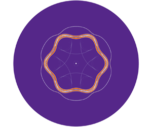
 $\alpha _0=1.111$) with initially unperturbed interfaces impacted by a concentric shock is first examined. The wave propagation and interface motions are visualized in figure 3. Note that the temporal origin is defined as the moment when the incident shock meets the outer interface. At the early moment ( $t=-0.042$), both the cylindrical incident shock (IS $_0$) and interfaces of the SF $_6$ layer are clearly identified in figure 3(a). As the IS $_0$ moves inward and collides with the outer interface II $_1$ (air–SF $_6$), the IS $_0$ bifurcates into an outward-moving reflected shock (RS $_1$) and an inward-moving transmitted shock (TS $_1$) as shown in figure 3(b). After that, the TS $_1$ collides with the inner interface II $_2$ (SF $_6$–air) and generates a second inward-moving transmitted shock (TS $_2$) and an outward-moving rarefaction wave (RW). Ascribed to the non-uniform flow field in the convergent geometry (Lombardini, Pullin & Meiron Reference Lombardini, Pullin and Meiron2014), the RW formed here remains sharp like a shock wave, which is consistent with the experimental results of Ding et al. (Reference Ding, Li, Sun, Zhai and Luo2019) and Sun et al. (Reference Sun, Ding, Zhai, Si and Luo2020). After impinging on the II $_1$, the RW reflects to form an inward-moving compression wave (CW) to collide with the II $_2$ as shown in figure 3(d). However, the formation of the CW and its collision with the II $_2$ are not presented in the experimental results with a larger radius ratio of $\alpha _0=1.833$ obtained by Ding et al. (Reference Ding, Li, Sun, Zhai and Luo2019) and Sun et al. (Reference Sun, Ding, Zhai, Si and Luo2020). This observation is attributed to the fact that the SF $_6$ layer is not thin enough in the experiment so that the reflected shock wave generated in the geometric centre impacts the SF $_6$ layer soon after the RW impinges the II $_1$. Due to the impact of the IS $_0$ on the SF $_6$ layer, the II $_1$ and II $_2$ move towards the geometric centre as shown in figure 3(c–f). As the TS $_2$ reaches the geometric centre, a reflected shock (RS $_2$) is generated immediately and moves outward away from the centre (see figure 3f). Later, the RS $_2$ impacts the II $_2$, which is called reshock, a well-known flow phenomenon happening in the convergent RM instability (Lombardini et al. Reference Lombardini, Pullin and Meiron2014; Wu et al. Reference Wu, Liu and Xiao2021). Consequently, the RS $_2$ bifurcates into an outward-moving transmitted shock (TS $_3$) and an inward-moving reflected shock (RS $_3$). Soon, the TS $_3$ colliding with the II $_1$ generates an outward-moving transmitted shock (TS $_4$) and reflects an inward-moving rarefaction wave (IRW) as shown in figure 3(h). It is clearly seen in figure 3(g,h) that both the II $_1$ and II $_2$ move outward after reshock.

Figure 3. (a–h) Wave propagation visualized by  $|\boldsymbol {\nabla }\rho |$ contours for the case that the convergent incident shock IS $_0$ impacts the unperturbed thin SF $_{6}$ layer with $\alpha _0=1.111$.
The quantitative descriptions for the positions of waves and interfaces and for the radial velocities ( $u_r$) of interfaces are displayed in figure 4. These descriptions are useful for the prediction of RT-unstable or RT-stable scenarios at the perturbed interfaces, depending on the interface type and acceleration direction of the interface (Lombardini et al. Reference Lombardini, Pullin and Meiron2014). Specifically, for the II $_1$ where the light fluid is placed outside, the interface is RT-unstable if it accelerates inward or decelerates outward (i.e. $\ddot r_1<0$); for the II $_2$ where the light fluid is inside, RT-unstable regions correspond to the interface decelerating inward or accelerating outward (i.e. $\ddot r_2>0$). As presented in figure 4(a), the II $_1$ and II $_2$ move inward from the static state immediately after being impacted by the IS $_0$ and TS $_1$, respectively. The collisions of the TS $_3$ with II $_1$ and the IRW with II $_2$ cause the interfaces to move outward. The radial velocities of the outward-moving interfaces are obviously slower than those of the inward-moving interfaces, which is the same as the experimental results (Ding et al. Reference Ding, Li, Sun, Zhai and Luo2019; Sun et al. Reference Sun, Ding, Zhai, Si and Luo2020). Furthermore, the temporal variations of the interfacial radial velocities are examined in figure 4(b). Three and two steps of $u_r$ appear before reshock as induced by the collisions of waves with the II $_1$ and II $_2$, respectively, and the differences of these steps of $u_r$ are listed in table 2. It is worth noting that the RW and CW obviously accelerate the II $_1$ and II $_2$ inward, and at this stage the perturbed II $_1$ and II $_2$ are RT-unstable and RT-stable, respectively. As displayed in figure 4(b), the II $_1$ has a third small velocity step at $t\approx 0.5$ when the second rarefaction wave (SRW) generated by the collision of the CW on II $_2$ impinges on II $_1$. However, the SRW is too weak to be identified via numerical schlieren images. The above phenomenon indicates that the waves generated by the incident shock wave sweeping through the thin SF $_6$ layer are critical in determining the interfacial radial velocities of the fluid layer. After $t\approx 0.7$, the II $_1$ and II $_2$ decelerating inward are RT-stable and RT-unstable, respectively. When the RS $_2$ and TS $_3$ impact the II $_2$ and II $_1$, respectively, the radial velocities of the inner and outer interfaces have sudden positive increases and their increase extents are listed in table 2. To clearly show the strength of the shocks impacting the interfaces, the shock Mach numbers of the incident shock colliding with the II $_1$ and II $_2$, and the shock Mach numbers of the reshock impacting the II $_1$ and II $_2$ are listed in table 2. At $t\approx 1.2$, as the IRW generated by the TS $_3$ impacting II $_1$ impinges the II $_2$, the radial velocity of the II $_2$ has another step and then both the II $_1$ and II $_2$ slowly move outward. The present results show the main features of the base flow of the convergent shock accelerating a thin heavy fluid layer, and will facilitate the analysis of the development of a perturbed layer.

Figure 4. Temporal variations of (a) the radial positions of interfaces and waves and of (b) the radial velocities of interfaces for the case that the convergent incident shock IS $_0$ impacts an unperturbed SF $_{6}$ layer with $\alpha _0=1.111$. Notation: II $_1$, outer interface; II $_2$, inner interface; RS $_i$,
$_i$,  $i$th reflected shock; TS $_i$,
$_i$,  $i$th transmitted shock; RW, rarefaction wave; CW, compression wave; SRW, second rarefaction wave; IRW, inward-moving rarefaction wave.
Table 2. Detailed parameters corresponding to the base flow. Here  $\Delta V_i$ is the difference of the $i$th step of $u_r$ before reshock and $\Delta V_r$ denotes the difference of $u_r$ induced by reshock; $Ma_i$ refers to the shock Mach number of incident shock colliding with the II $_1$ and II $_2$; and $Ma_r$ refers to the shock Mach number of reshock colliding with the II $_1$ and II $_2$.
$_2$.

3.2. Instability evolution of the perturbed thin SF$_6$ layer

Next, two typical cases of the perturbed thin SF $_6$ layer with $\alpha _0=1.111$, namely the ‘Outer’ case consisting of a cosinoidal outer interface and a circular inner interface and the ‘Inner’ case where the unperturbed outer interface and cosinoidal inner interface are composed, are examined to investigate the instability evolution of the thin heavy fluid layer. The perturbation wavenumber of these two cases is set as $n=6$, which is consistent with the previous experimental setting (Ding et al. Reference Ding, Li, Sun, Zhai and Luo2019; Sun et al. Reference Sun, Ding, Zhai, Si and Luo2020). The initial amplitude of the perturbed outer interface for the Outer case is $a_1=0.02\lambda _1$, where $\lambda _1=2{\rm \pi} r_1/n$ is the perturbation wavelength of the II $_1$. Considering that the collision of a shock wave from heavy to light fluids on the perturbed interface causes reverse growth of the perturbation, the initial amplitude of the perturbed inner interface for the Inner case is set as $a_2=-0.02\lambda _2$, with $\lambda _2=2{\rm \pi} r_2/n$ denoting the perturbation wavelength of the II $_2$, to ensure that the perturbation growth is in phase with that in the Outer case. The simulations are carried out on three grids of size $600^2$ (coarse), $900^2$ (intermediate) and $1200^2$ (fine), which are uniform in both radial and circumferential directions, and evolutions for the perturbation amplitudes are displayed in figure 5. The perturbation amplitude $\eta _i$ is defined as $\eta _i=(r_{\theta =0}-r_{\theta ={\rm \pi} /n})/2$ $(i=1,2)$, with $r_{\theta =0}$ and $r_{\theta ={\rm \pi} /n}$ representing the radii of the locations where $Y_A=0.5$ along $\theta =0$ and $\theta ={\rm \pi} /n$ lines, respectively. In this way, the phase reversal in the perturbation growth can be observed (see figure 5b). The converged results depicted in figure 5 confirm that the present simulations are reliable for capturing the essential flow dynamics in instability evolution of the shock-accelerated perturbed thin SF $_6$ layer. In the following, to obtain the fine flow field for the purpose of clear visualization of morphologies of the interfaces and waves, all the discussion of results and analysis concern the simulations of the fine grid resolution ( $1200^2$).

Figure 5. Temporal evolutions of the amplitudes for the perturbed SF $_6$ layers in (a) the Outer case and in (b) the Inner case with three grid resolutions: $600^2$ (red solid lines), $900^2$ (green dashed lines) and $1200^2$ (blue dot-dashed lines). The lines with triangles represent the amplitude of the outer interface and lines with circles denote the amplitude of the inner interface. The coloured long-dashed and double-dot-dashed lines are the results calculated by the compressible Bell model (Wu et al. Reference Wu, Liu and Xiao2021).
The underlying physical mechanisms of the perturbation growth presented in figure 5(a) can be interpreted by the numerical schlieren images for the Outer case shown in figure 6. Initially, the IS $_0$ together with the II $_1$ and II $_2$ can be clearly identified (see figure 6a). As the IS $_0$ moves inward, it first collides with the cosinoidally perturbed II $_1$, resulting in a perturbed TS $_1$ moving inward and a perturbed RS $_1$ moving outward, and both the TS $_1$ and RS $_1$ have the same phase as the II $_1$. It is worth noting that there is a sudden decrease in $\eta _1$ at $t=0$, attributed to the fact that the inward-moving IS $_0$ first encounters the crest of the II $_1$ which consequently obtains an inward radial velocity, while the rest of the II $_1$ remains still. This radial velocity difference produces a sudden decrease of $\eta _1$, which is called the compression effect of the IS $_0$ (Richtmyer Reference Richtmyer1960). After $t=0$ when the IS $_0$ collides with the II $_1$, the perturbation on the II $_1$ grows as driven by the RM instability as shown in figure 5(a). Later, the TS $_1$ impacts the II $_2$ and bifurcates into a perturbed RW in inverse phase with respect to the II $_1$ and a perturbed TS $_2$ in the same phase as the II $_1$ (see figure 6c). Due to the TS $_1$ impacting II $_2$, a small perturbation is introduced to the II $_2$ and then grows slowly in the same phase as the II $_1$ (Zou et al. Reference Zou, Al-Marouf, Cheng, Samtaney, Ding and Luo2019). Specifically, the trough of the inward-moving perturbed TS $_1$ first encounters the II $_2$ whose corresponding part consequently obtains an inward radial velocity, while the rest of the II $_2$ remains still. This radial velocity difference produces a sudden increase of $\eta _2$ from $t\approx 0.13$ to $t\approx 0.17$ and thus the TS $_1$ causes a decompression effect on II $_2$. After being impinged by the RW, the perturbation on the II $_1$ has a short-term rapid increase from $t\approx 0.22$ to $t\approx 0.30$ under the decompression effect of the RW. The reasons for the decompression effect of the RW on II $_1$ are as follows. The RW first encounters the trough of the II $_1$ whose inward radial velocity is accelerated to a greater value due to the fact that the pressure behind the RW front is lower than that before the RW front (Liang et al. Reference Liang, Liu, Zhai, Si and Wen2020). However, the crest of the II $_1$ still keeps its original radial velocity. This radial velocity difference produces the sudden increase of $\eta _1$ from $t\approx 0.22$ to $t\approx 0.30$. Then as shown in figure 6(d) the perturbed CW reflected by the collision of the RW on II $_1$ impacts the II $_2$, which makes the perturbation on the II $_2$ increase rapidly. After $t\approx 0.4$ when the CW passes through the II $_2$, both the II $_1$ and II $_2$ move inward and the perturbations increase continuously as driven by the RM instability and the convergence effect (BP effect). It is of interest that the shape of the TS $_2$ at $t=0.636$ becomes almost hexagonal with a phase opposite to that at $t=0.317$. This observation is consistent with the behaviours predicted by Schwendeman & Whitham (Reference Schwendeman and Whitham1987) using an approximate theory of shock dynamics. As the TS $_2$ reaches the geometric centre, the outward-moving perturbed RS $_2$ is generated, and the RS $_2$ is in phase with respect to the II $_2$ at $t=0.931$. After the RS $_2$ impacts the II $_2$, the perturbation on the II $_2$ decreases slightly under the compression effect of the RS $_2$, and then increases continuously due to the RM instability as shown in figure 5(a). Soon, the perturbed TS $_3$ generated by the RS $_2$ impacting on II $_2$ collides with the II $_1$, and as shown in figure 5(a) the perturbation on the II $_1$ grows in the opposite direction after $t\approx 1.1$ due to the RM instability with the shock travelling from heavy to light fluids. Especially, the spike structure formed on the II $_1$ grows in a direction opposite to that formed on the II $_2$ at $t=1.498$ as presented in figure 6(i).

Figure 6. (a–i) Wave propagation visualized by the  $|\boldsymbol {\nabla }\rho |$ contours for the Outer case.
For the Outer case, a very interesting and noteworthy phenomenon in the instability evolution of the thin SF $_6$ layer is that the inner interface grows in the same phase as the outer interface before the SF $_6$ layer is re-accelerated by reshock. This behaviour is different from the inverse phase growth of the inner interface compared with the outer interface in the instability evolution of the thick SF $_6$ layer (Ding et al. Reference Ding, Li, Sun, Zhai and Luo2019). In order to explain this difference between the cases of the thin and thick fluid layers, it is necessary to clarify the evolution mechanism of the interface after the convergent perturbed shock impacts the circular interface. According to a previous study (Zou et al. Reference Zou, Al-Marouf, Cheng, Samtaney, Ding and Luo2019), the problem of the perturbed shock impacting on the unperturbed interface in convergent geometry is a non-standard RM instability where the baroclinic mechanism is somewhat insignificant. In fact, the pressure perturbation and cylindrical BP effect contribute most significantly to the deformed shock-induced RM instability (Zou et al. Reference Zou, Al-Marouf, Cheng, Samtaney, Ding and Luo2019). To this end, the growth rate of the perturbation amplitude of the II $_2$ after $t=t_{TS_1}$ when the perturbed TS $_1$ impacts the II $_2$ can be expressed as (Zou et al. Reference Zou, Al-Marouf, Cheng, Samtaney, Ding and Luo2019)
 \begin{equation} \dot\eta_2=\varepsilon\frac{|\Delta V_1|}{V_{s, t=t_{TS_1}}}\dot\eta_{s, t=t_{TS_1}}+\frac{|\Delta V_1|}{r_2}\eta_{2,t=t_{TS_1}}. \end{equation}
The first term on the right-hand side of the above equation represents the contribution of the pressure perturbation which can be further divided into impulsive perturbation and continuous perturbation (Zou et al. Reference Zou, Al-Marouf, Cheng, Samtaney, Ding and Luo2019). Here,  $\varepsilon$ is a dimensionless parameter and $1-\varepsilon$ stands for the ratio of the continuous perturbation to the impulsive perturbation, $\Delta V_1$ is the radial velocity difference of the II $_2$ induced by the circular TS $_1$ and is listed in table 2, $V_{s,t=t_{TS_1}}$ represents the radial velocity of the circular TS $_1$ at $t=t_{TS_1}$ and $\dot \eta _{s,t=t_{TS_1}}$ denotes the perturbation growth rate of the perturbed TS $_1$ at $t=t_{TS_1}$. The contribution of the cylindrical BP effect is represented by the second term on the right-hand side of (3.1) in which $\eta _{2,t=t_{TS_1}}$ is the amplitude of the perturbation on the II $_2$ introduced by the TS $_1$ at $t=t_{TS_1}$ and $r_2$ denotes the radial location of the II $_2$. The temporal variation of the amplitude of the TS $_1$ is plotted in figure 7 to obtain $\dot \eta _{s,t=t_{TS_1}}$ in (3.1). It is clearly seen that for the Outer case of the thin SF $_6$ layer (i.e. $\alpha _0=1.111$), $\dot \eta _{s,t=t_{TS_1}}\approx 0$, which means that the only contribution of $\dot \eta _2$ is from the cylindrical BP effect and is positive. Thus, after being impacted by the TS $_1$, the II $_2$ of the thin SF $_6$ layer keeps the same phase growth as the II $_1$, and then the perturbed CW accelerating the inward movement of the II $_2$ makes the perturbation on the II $_2$ grow rapidly. With the thickening of the initial SF $_6$ layer, $\dot \eta _{s,t=t_{TS_1}}$ decreases gradually and is negative. For example, when $\alpha _0=2$, $\dot \eta _{s,t=t_{TS_1}}\approx -0.019$. In addition, based on the facts that $\eta _{2,t=t_{TS_1}}$ of the thick SF $_6$ layer decreases due to the decrease of the perturbation amplitude of the inward-moving TS $_1$ and that the value of $\varepsilon$ in (3.1) is approximately $1$ (Zou et al. Reference Zou, Al-Marouf, Cheng, Samtaney, Ding and Luo2019), $\dot \eta _2$ of the thick SF $_6$ layer (i.e. $\alpha _0 = 2$) is dominated by the pressure perturbation and is negative. Therefore, $\eta _2$ of the thick SF $_6$ layer in the same phase at $t=t_{TS_1}$ with $\eta _1$ is reversed rapidly at a negative growth rate, and the II $_2$ and II $_1$ are in inverse phase. This result is also obtained in previous experimental work (Ding et al. Reference Ding, Li, Sun, Zhai and Luo2019).

Figure 7. The amplitudes of the TS $_1$ versus time for the Outer case with $\alpha _0=1.111$, $\alpha _0=2$ and $\alpha _0=\infty$ (only the outer interface). The amplitude $\eta _s$ is defined as $\eta _s= (r_{\theta =0}-r_{\theta ={\rm \pi} /6})/2$, with $r_{\theta =0}$ and $r_{\theta ={\rm \pi} /6}$ representing the radial points where the TS $_1$ intersects with lines $\theta =0$ and $\theta ={\rm \pi} /6$, respectively. The tangent lines are given at the moment when the TS $_1$ impacts the II $_2$.
$_2$.
The acceleration of the shock on the thin SF $_6$ layer also causes the instability evolution of the interfaces for the Inner case as shown in figure 5(b), which can be further examined by the numerical schlieren images in figure 8. Attributed to the II $_1$ without perturbation, the IS $_0$, RS $_1$ and TS $_1$ still keep a circular shape with no perturbation introduced before the collision of the TS $_1$ with the cosinoidal II $_2$. As time proceeds, the TS $_1$ collides with the II $_2$, generating a perturbed TS $_2$ in a phase opposite to that of the initial II $_2$ and a perturbed RW in the same phase as the initial II $_2$. The above phenomena were also found in a previous experiment (Sun et al. Reference Sun, Ding, Zhai, Si and Luo2020) and the reason for the anti-phase TS $_2$ is interpreted as follows. The inward-moving TS $_1$ first encounters the crest of the cosinoidal II $_2$ and then a part of the TS $_1$ transmits into the air attaining a higher travelling speed. While the rest of the TS $_1$ continues to propagate in SF $_6$ at a lower speed. This radial velocity difference produces an anti-phase perturbation on the TS $_2$. In addition, due to the impingement of the TS $_1$ on II $_2$, the initial negative $\eta _2$ has an instantaneous increase at $t\approx 0.15$ under the compression effect of the TS $_1$, and then grows slowly as driven by the RM instability and BP effect. After the perturbed RW impinging on the II $_1$, a perturbation amplitude in inverse phase with respect to the RW is introduced on the II $_1$, and then grows due to the cylindrical BP effect caused by the inward movement of the II $_1$. However, the impingement of the RW does not obviously cause the instability evolution on the II $_1$ of the thick SF $_6$ layer with $\alpha _0=1.833$ (Sun et al. Reference Sun, Ding, Zhai, Si and Luo2020), due to the reduction of the perturbation on the RW after a long-distance outward movement in the thick fluid layer. Later, the perturbed CW reflecting from the II $_1$ and moving inward impacts the II $_2$, speeding up the growth of $\eta _2$ so that $\eta _2$ increases quickly over zero. After $t\approx 0.4$, the II $_1$ and II $_2$ grow in the same phase until the RS $_2$ reflected from the geometric centre reshocks the SF $_6$ layer. The instability evolution after reshock in the Inner case is the same as that in the Outer case, namely the perturbation of the II $_2$ increases continuously and the perturbation of the II $_1$ decreases.

Figure 8. (a–i) Wave propagation visualized by the  $|\boldsymbol {\nabla }\rho |$ contours for the Inner case.
For the Outer and Inner cases, the instabilities on both the II $_1$ and II $_2$ have a significant increase before reshock. In groundbreaking work, Bell (Reference Bell1951) employed a potential flow model to describe the instability growth on a thick cylindrical shell in vacuum, where the shell can be either incompressible or uniformly compressing. Later, Epstein (Reference Epstein2004) extended the Bell model to the fluid–fluid case assuming two uniformly compressing fluids which are compressing at the same rate (i.e. the Atwood number does not change). Here, we examine whether this compressible Bell model capturing well the perturbation growth of the thick cylindrical layer (Ding et al. Reference Ding, Li, Sun, Zhai and Luo2019) can describe the instability evolution of the thin SF $_6$ layer considered here. Under a small-perturbation assumption, the simplified compressible Bell model takes the form (Bell Reference Bell1951; Epstein Reference Epstein2004)
 \begin{equation} \dot\eta_{i}=\dot\eta_{i,RM}+\dot\eta_{i,RT}+\dot\eta_{i,Com}, \end{equation}
where the single dot denotes the first derivative with respect to time  $t$,
$t$,  $\dot \eta _{i,RM}$ represents the perturbation growth rate due to the RM instability with the BP effect, $\dot \eta _{i,RT}$ is the growth rate contributed by the RT stability/instability with the BP effect and $\dot \eta _{i,Com}$ denotes the growth rate caused by the compressibility effect that refers to the effect of fluid compression caused by the basic flow to the centre (Epstein Reference Epstein2004; Luo et al. Reference Luo, Li, Ding, Zhai and Si2019). Note that the BP effect is coupled into each of the above terms and difficult to isolate from others (Wu et al. Reference Wu, Liu and Xiao2021). The above three contributions to the perturbation growth rate are expressed as (Epstein Reference Epstein2004; Wu et al. Reference Wu, Liu and Xiao2021)
 \begin{gather} \dot\eta_{i,RM} = \frac{r_{i,t=t_j^+}^2\dot\eta_{i,t=t_j^+}}{r_i^2(t)}, \end{gather}
 \begin{gather}\dot\eta_{i,RT} ={-}\frac{nA_{T,i}+1}{r_i^2(t)}\int_{t_{0}}^{t} r_i(\tau)\ddot r_i(\tau)\eta_i(\tau)\,\mathrm{d}\tau, \end{gather}
 \begin{gather}\dot\eta_{i,Com} = \frac{c_i}{r_i^2(t)}\left[\int_{t_{0}}^{t} r_i(\tau)\dot r_i(\tau)\eta_i(\tau)\,\mathrm{d}\tau +\int_{t_{0}}^{t} r_i^2(\tau)\dot\eta_i(\tau)\,\mathrm{d}\tau\right]. \end{gather}
Here,  $i=1$ and $2$ corresponding to the II $_1$ and II $_2$, respectively, $r_{i,t=t_j^+}$ and $\dot \eta _{i,t=t_j^+}$ represent the position and growth rate of the $i$th interface at the end moment $t_j^+$ of the $j$th wave passing through the interface, respectively, and $A_{T,i}=(\rho _{i,in}-\rho _{i,out})/(\rho _{i,in}+\rho _{i,out})$ is the post-shock Atwood number at the $i$th interface with $\rho _{i,in}$ and $\rho _{i,out}$ representing the inner and outer fluid densities, respectively. The parameter $c_i=-\dot {\rho }_{i,in}/\rho _{i,in}=-\dot {\rho }_{i,out}/\rho _{i,out}$ in (3.3c) characterizes the expansion rate of the species at the $i$th interface, which can be approximated as a constant value, $c_i\approx [(r_{i,min}/r_{i,0})^2-1]/t_{res}$ (Luo et al. Reference Luo, Li, Ding, Zhai and Si2019; Wu et al. Reference Wu, Liu and Xiao2021). Here, $r_{i,min}$ denotes the smallest radius of the $i$th interface during its motion, $r_{i,0}$ is the initial position of the $i$th interface and $t_{res}$ represents the time when the reshock happens. Note that the significant deviations between the compressible Bell model and the DNS results before reshock are presented in figure 5, and the reasons of these deviations are as follows. On the one hand, the compression/decompression effect of the impingement of the waves on the interface cannot be described by the compressible Bell model. For example, in the Outer case, this model fails to capture the rapid increase of $\eta _1$ when $t\approx 0.22\sim 0.30$ under the decompression effect of the RW. On the other hand, attributed to the fact that $\alpha ^n<6~(\alpha =r_1/r_2)$ in the present study, the interface coupling effect and thin-shell correction are critical to the perturbation growth and must be considered (Zhang et al. Reference Zhang, Liu, Kang, Xiao, Tao, Zhang, Zhang and He2020). Therefore, the neglect of the interface coupling effect and thin-shell correction also makes the compressible Bell model deviate from the DNS results.
3.3. Model for the instability evolution of the thin SF$_6$ layer

According to the detailed analysis in the previous subsection, improvement in the compressible Bell model is required to capture the instability evolution of the thin heavy fluid layer, by including new terms to describe the contributions of interface coupling effect, thin-shell correction and compression/decompression effect of waves. Based on the potential flow theory, Zhang et al. (Reference Zhang, Liu, Kang, Xiao, Tao, Zhang, Zhang and He2020) gave for the first time the mathematical forms of the interface coupling effect and thin-shell correction for a thin cylindrical incompressible fluid shell in vacuum, which are included in the equations for  $\eta _{1}$ and $\eta _{2}$ as (Zhang et al. Reference Zhang, Liu, Kang, Xiao, Tao, Zhang, Zhang and He2020)
 \begin{align} &\frac{\mathrm{d}(r_1^2\dot\eta_1)}{\mathrm{d}t} +(n+1)\ddot r_1r_1\eta_1 + \frac{2n}{\alpha^{2n}-1}\ddot r_1r_1\eta_1\nonumber\\ &\qquad=\frac{2n\alpha^{n+1}}{\alpha^{2n}-1}\ddot r_1r_1\eta_2 +\frac{2n\alpha^{n-1}(\alpha^2-1)}{\alpha^{2n}-1}\dot r_1r_1\dot\eta_2, \end{align}
 \begin{align} &\frac{\mathrm{d}(r_2^2\dot\eta_2)}{\mathrm{d}t} -(n-1)\ddot r_2r_2\eta_2 - \frac{2n}{\alpha^{2n}-1}\ddot r_2r_2\eta_2\nonumber\\ &\qquad={-}\frac{2n\alpha^{n-1}}{\alpha^{2n}-1}\ddot r_2r_2\eta_1+\frac{2n\alpha^{n-1}(\alpha^2-1)}{\alpha^{2n}-1}\dot r_2r_2\dot\eta_1, \end{align}
respectively, where  $\alpha =r_1/r_2$ and the dot and double dots denote the first and second derivatives with respect to time $t$, respectively. The first two terms on the left-hand side of (3.4) and (3.5) represent the incompressible Bell model (Bell Reference Bell1951), and the temporal integrals of these two terms are exactly the same as (3.2) in which $|A_{T,i}|=1$ and the terms of compressibility effect are not included. The third terms on the left-hand side of (3.4) and (3.5) represent the thin-shell corrections (Zhang et al. Reference Zhang, Liu, Kang, Xiao, Tao, Zhang, Zhang and He2020). When the thickness of the layer decreases leading to $\alpha \rightarrow 1$, the thin-shell correction becomes important. The terms of the interface coupling effect on the right-hand side of (3.4) and (3.5) are roughly of the order of $\alpha ^{-n}$ for large $\alpha$, namely these coupling terms can be ignored for the thick fluid layer. They can be further divided into amplitude coupling terms and velocity coupling terms corresponding to, respectively, the first and second terms on the right-hand side of (3.4) and (3.5) (Zhang et al. Reference Zhang, Liu, Kang, Xiao, Tao, Zhang, Zhang and He2020).
In fact, the above model given by Zhang et al. (Reference Zhang, Liu, Kang, Xiao, Tao, Zhang, Zhang and He2020) can be regarded as an extension of the original Bell model (Bell Reference Bell1951), that is, the coupling terms and thin-shell correction have been added to predict the perturbation growth of the thin fluid layer in vacuum. For the current heavy fluid layer, the density of SF $_6$ is much higher than that of air and the absolute values of Atwood number are as large as $0.67$ close to $1$. Based on the small-perturbation assumption under which the perturbation obeys linear growth, the temporal integral forms of the thin-shell correction and the coupling terms in (3.4) and (3.5) are superimposed on (3.2), i.e.
 \begin{equation} \dot\eta_i=\dot\eta_{i,RM}+\dot\eta_{i,RT}+\dot\eta_{i,Com}+\dot\eta_{i,Thin}+\dot\eta_{i,Cou}, \end{equation}
to improve the compressible Bell model so that it can describe the instability evolution of the thin SF $_6$ layer. Here, $\dot \eta _{i,Thin}$ and $\dot \eta _{i,Cou}$ represent the contributions of the thin-shell correction and the interface coupling effect to the growth rate of the perturbation on the $i$th interface, respectively. Term $\dot \eta _{i,Thin}$ takes the form
 \begin{equation} \dot\eta_{i,Thin}=\frac{({-}1)^i}{r_i^2(t)}\int_{t_{0}}^{t} \frac{2n}{\alpha^{2n}(\tau)-1} \ddot r_i(\tau)r_i(\tau)\eta_i(\tau)\,\mathrm{d}\tau, \end{equation}
and the forms of  $\dot \eta _{1,Cou}$ and $\dot \eta _{2,Cou}$ are expressed as
 \begin{align} \dot\eta_{1,Cou}& = \frac{1}{r_1^2(t)} \left\{\int_{t_{0}}^{t} \frac{2n\alpha^{n+1}(\tau)}{\alpha^{2n}(\tau)-1} \ddot r_1(\tau)r_1(\tau)\eta_2(\tau)\,\mathrm{d}\tau \right. \nonumber\\ &\quad \left. +\int_{t_{0}}^{t}\frac{2n\alpha^{n-1}(\tau)[\alpha^2(\tau)-1]}{\alpha^{2n}(\tau)-1} \dot r_1(\tau)r_1(\tau)\dot\eta_2(\tau)\,\mathrm{d}\tau \right\} \end{align}
and
 \begin{align} \dot\eta_{2,Cou}& = \frac{1}{r_2^2(t)} \left\{-\int_{t_{0}}^{t} \frac{2n\alpha^{n-1}(\tau)}{\alpha^{2n}(\tau)-1} \ddot r_2(\tau)r_2(\tau)\eta_1(\tau)\,\mathrm{d}\tau \right. \nonumber\\ &\quad \left. +\int_{t_{0}}^{t}\frac{2n\alpha^{n-1}(\tau)[\alpha^2(\tau)-1]}{\alpha^{2n}(\tau)-1} \dot r_2(\tau)r_2(\tau)\dot\eta_1(\tau)\,\mathrm{d}\tau \right\}, \end{align}
respectively. On the one hand, when  $A_{T,1}=1$ and $A_{T,2}=-1$, (3.6) without the compressibility effect term recovers the model of Zhang et al. (Reference Zhang, Liu, Kang, Xiao, Tao, Zhang, Zhang and He2020). On the other hand, with the fluid layer thickening, i.e. $\alpha \rightarrow \infty$, (3.6) can be reduced to the compressible Bell model, i.e. (3.2). The above analysis points to that (3.6) can be viewed in physics as a rational combination of the compressible Bell model describing the single interface of arbitrary $A_T$ with the model of Zhang et al. (Reference Zhang, Liu, Kang, Xiao, Tao, Zhang, Zhang and He2020) predicting the evolution of the cylindrical fluid layer in vacuum. Therefore, (3.6) needs to satisfy all the three assumptions involved in these two models, i.e. the small-amplitude assumption, potential flow assumption (Epstein Reference Epstein2004; Zhang et al. Reference Zhang, Liu, Kang, Xiao, Tao, Zhang, Zhang and He2020) and uniformly compressing assumption (Epstein Reference Epstein2004).
As shown in figures 6 and 8, the interfaces of the shock-accelerated thin fluid layer are successively impacted by several waves, and the overall variations of the perturbation amplitudes on the interfaces caused by the compression/decompression effects of the successive waves can be obtained by accumulating every rapid decrease/increase of the amplitude induced by each wave. For the compression effect of one known wave, for example, a shock wave compressing a perturbed interface (Richtmyer Reference Richtmyer1960), the decrease of the amplitude is usually estimated by
 \begin{equation} \eta^+{-}\eta^-{=}-\frac{|\Delta V_W|T_W}{2}, \end{equation}
where  $\eta ^+$ and $\eta ^-$ are the amplitudes after and before this wave impacting, respectively, $\Delta V_W$ represents the radial velocity step of the circular interface caused by this wave and $T_W=2\eta ^-/V_W$ denotes the time for this wave to travel from the interfacial crest to trough with a constant speed $V_W$ (Wu et al. Reference Wu, Liu and Xiao2021). Consequently, it leads to a perturbation compression rate $\eta ^+/\eta ^-=1-|\Delta V_W|/V_W$ (Richtmyer Reference Richtmyer1960; Meshkov Reference Meshkov1969; Wu et al. Reference Wu, Liu and Xiao2021). The accuracy of (3.10) can be verified by the compression rates of the II $_1$ impacted by the IS $_0$ in the Outer case and the II $_2$ collided by the TS $_1$ in the Inner case. When the IS $_0$ impacts the II $_1$ as shown in figure 5(a), $\Delta V_W$ of the II $_1$ is $\Delta V_1$ listed in table 2 and $V_W$ of the IS $_0$ is $1.480$ which is the absolute value of the slope of the IS $_0$ position curve in figure 4. Thus, the calculated compression rate of the II $_1$ is $0.777$. In addition, because $\eta _{1}$ decreases rapidly from $0.0209$ to $0.0161$ at $t\approx 0$ when the IS $_0$ impacts the II $_1$, the compression rate can also be measured directly as $0.0161/0.0209\approx 0.770$. Similarly, the compression rate of the II $_2$ collided by the TS $_1$ in the Inner case is calculated as $0.319$ and directly measured as $0.310$. The above compression rates measured directly are very close to those calculated using (3.10), which proves that (3.10) can reliably model the amplitude decrease caused by the compression effect of one known wave. In fact, (3.10) has also been verified and adopted by recent experimental (Ding et al. Reference Ding, Si, Yang, Lu, Zhai and Luo2017) and numerical (Wu et al. Reference Wu, Liu and Xiao2021) studies. Furthermore, (3.10) can also estimate the amplitude increase under the decompression effect of a wave by replacing the minus sign on the right-hand side of (3.10) with a plus sign (Liang & Luo Reference Liang and Luo2021). Note that the amplitude of the interface varies linearly with time under the compression/decompression effect of a wave, so (3.10) can describe the time-varying compression/decompression effect by replacing the time variable $t$ with $T_W$ (Liang & Luo Reference Liang and Luo2021). To this end, the time-varying compression/decompression effect (Richtmyer Reference Richtmyer1960; Liang & Luo Reference Liang and Luo2021) including each wave impacting the $i$th interface $\eta _{i,CD}(t)$ can be modelled as
 \begin{equation} \eta_{i,CD}(t)=\eta_{i,t_0}+\int_{t_0}^{t}\frac{\Delta V(\tau)}{2} \,\mathrm{d}\tau, \end{equation}
where  $\eta _{i,t_0}$ is the initial amplitude of the $i$th interface at $t=t_0$. The function $\Delta V(\tau )$ defined in (3.11) represents the radial velocity step of the circular interface at the moment $\tau$, namely if $t_j^-<\tau < t_j^+$, $\Delta V(\tau )=\pm |\Delta V_j|$, otherwise $\Delta V(\tau )=0$. Here, $\Delta V_j$ is the $j$th radial velocity step listed in table 2, $t_j^-$ and $t_j^+$ are the beginning and end moments of the $j$th wave passing through the interface and the operators ‘ $+$’ and ‘ $-$’ before the term $|\Delta V_j|$ represent decompression and compression effects. Parameters $t_j^-$ and $t_j^+$ can be obtained directly from the numerical results. For example, when the perturbed RW impinges the II $_1$ in the Outer case, $\eta _1$ increases rapidly in the time range from $t\approx 0.22$ to $0.30$ under the decompression effect of the RW as shown in figure 5(a). Thus, for the RW passing through the II $_1$,
$_1$,  $t_j^-\approx 0.22$ and $t_j^+\approx 0.30$. The reverberated waves resulting in the compression/decompression effects modelled by (3.11) are caused by the IS $_0$ impacting the fluid layer. However, (3.6) based on the potential flow assumption appears independent of whether there is an IS $_0$ and does not involve the process of wave–interface collision. Therefore, (3.6) excludes the compression/decompression effects of the reverberated waves colliding with the interfaces. By adding (3.11) to the temporal integral of (3.6), the compressible Bell model is further improved and the perturbation amplitude $\eta _i$ of the $i$th interface of the SF $_6$ layer can be completed as the following model:
 \begin{equation} \eta_i=\eta_{i,RM}+\eta_{i,RT}+\eta_{i,Com}+\eta_{i,Thin}+\eta_{i,Cou}+\eta_{i,CD}. \end{equation}
 To verify the reliability of the improved compressible Bell model, for the Outer case, the temporal variations of the perturbation amplitudes calculated by the model (3.12) before reshock are presented and compared with the DNS results in figure 9. One should keep in mind that the improved model (3.12) is also based on the small-amplitude assumption adopted by the Bell model and, therefore, is unable to predict large-amplitude growth of perturbation after reshock, i.e.  $t\gtrsim 1.0$. Parameters $r_{i,t=t_j^+}$ and $\dot \eta _{i,t=t_j^+}$ required to calculate the $\eta _{i,RM}$ term of the model (3.12) according to (3.3a) are obtained by DNS results and listed in table 3. Specifically, the contributions of the impingements of the IS $_0$, RW and SRW on the II $_1$ to the perturbation growth rate are considered, and the contributions of the TS $_1$ and CW to the perturbation growth rate of the II $_2$ are taken into account. For the II $_1$,
$_1$,  $A_{T,1}$ required for calculating the term $\eta _{1,RT}$ and $c_1$ required to calculate the term $\eta _{1,Com}$ are obtained from the base flow as $0.708$ and $-0.657$, respectively. Whereas for the II $_2$,
$_2$,  $A_{T,2}=-0.698$ and $c_2=-0.776$. The improved compressible Bell model (3.12) agrees well with the DNS result of the II $_1$ before reshock. For the II $_2$, the improved model captures well the behaviours of the perturbation growth until $t\approx 0.7$ when the II $_2$ decelerates inward and then slightly underestimates the DNS results. This underestimation is caused by the thin-shell correction and interface coupling effect which are obtained by the model of Zhang et al. (Reference Zhang, Liu, Kang, Xiao, Tao, Zhang, Zhang and He2020) aimed at a thin fluid layer in vacuum. However, compared with the compressible Bell model (3.2), the improved model shows a better prediction of the instability evolution before $t\approx 0.7$.

Figure 9. The perturbation amplitudes of the outer (a) and inner (b) interfaces along with their decomposed contribution terms versus time for the Outer case before reshock. The simulation data marked by symbols are added for comparison.
Table 3. The parameters required for calculating the terms like  $\dot \eta _{i,RM}$ and $\eta _{i,CD}$ are obtained by DNS results in the Outer case. Here, $t_j^-$ and $t_j^+$ are the beginning and end moments of the $j$th wave passing through the interface and $r_{i,t=t_j^+}$ and $\dot \eta _{i,t=t_j^+}$ represent the position and growth rate of the II $_i$ at $t=t_j^+$, respectively.

It is clearly seen in figure 9 that the growths of perturbations on both the II $_1$ and II $_2$ are dominated by the RM instability. Term $\eta _{1,RT}$ increases before $t\approx 0.7$ due to the fact that the II $_1$ is RT-unstable under the inward acceleration of the RW. Attributed to the deceleration of the II $_1$ and II $_2$ after $t\approx 0.7$, the II $_1$ becomes RT-stable and $\eta _{1,RT}$ decreases, while the II $_2$ is RT-unstable and $\eta _{2,RT}$ increases. This significant difference of $\eta _{1,RT}$ and $\eta _{2,RT}$ is attributed to the interface type (Lombardini et al. Reference Lombardini, Pullin and Meiron2014), i.e. the light–heavy (II $_1$) and heavy–light (II $_2$) interfaces. Both $\eta _{1,Com}$ and $\eta _{2,Com}$ decrease with time and thus the compressibility effect suppresses the perturbation growth on the interfaces, which is the same behaviour as the experimental result of a shock-accelerated interface in cylindrical geometry (Luo et al. Reference Luo, Li, Ding, Zhai and Si2019). It is particularly important that the thin-shell correction $\eta _{i,Thin}$ and interface coupling effect $\eta _{i,Cou}$ contribute significantly to the instability evolution of the current thin SF $_6$ layer. The temporal trend of $\eta _{i,Thin}$ behaves similar to that of $\eta _{i,RT}$, resulting from that $\ddot r_ir_i\eta _i$ is included in both mathematical forms. However, the contribution of $\eta _{1,Thin}$ in the Outer case is stronger than that of $\eta _{1,RT}$ to the perturbation growth at the II $_1$ where the initial perturbation is introduced. The interface coupling effect $\eta _{1,Cou}$ suppresses the perturbation growth of the II $_1$ until $t\approx 0.95$ close to the reshock and then slightly promotes the instability evolution. Nevertheless, the interface coupling effect always suppresses the growth of perturbation on the II $_2$ before reshock. Note that $\eta _{i,Cou}$ depends on not only the motion of the interface itself (like other terms) but also the perturbation at another interface. Therefore, one could expect that the difference of $\eta _{1,Cou}$ and $\eta _{2,Cou}$ comes from the complex coupling between II $_1$ and II $_2$. In addition, $\eta _{i,CD}$ well captures the rapid decrease/increase of perturbation amplitude under the compression/decompression effect of the waves impacting the interfaces. Specifically, the compression effect of the IS $_0$ causes a sudden decrease of the perturbation on the II $_1$ at $t\approx 0$ and the decompression effect of the RW at $t\approx 0.25$ leads to an increase of the perturbation on the II $_1$. For the II $_2$, the decompression effects of the TS $_1$ and CW result in increases of perturbation at $t\approx 0.15$ and $t\approx 0.35$, respectively. Note that the decompression effect of the SRW on the II $_1$ is negligibly weak. Obviously, the great difference of $\eta _{1,CD}$ and $\eta _{2,CD}$ results from that the types of waves colliding with the II $_1$ and II $_2$ are different and the collision times are also different.
Furthermore, as shown in figure 10, the improved compressible Bell model is also employed to evaluate the contribution of each effect to the perturbation growth before reshock in the Inner case. Parameters  $r_{i,t=t_j^+}$ and $\dot \eta _{i,t=t_j^+}$ required to calculate the $\eta _{i,RM}$ term for the Inner case are listed in table 4. Sharing the same base flow, the Inner case has the same $A_{T,i}$ and $c_i$ as the Outer case. As presented in figure 10, the improved compressible Bell model (3.12) also shows a good agreement for the II $_1$ and for the II $_2$ before $t\approx 0.7$. The RM instability also dominates the perturbation growth in the Inner case. Because the basic flow is the same for the Outer and Inner cases, both $\eta _{i,RT}$ accounting for the RT stability/instability and $\eta _{i,Com}$ characterizing the compressibility effect have the same trends of temporal variation in the two cases. In the Inner case, the temporal variation of $\eta _{i,Thin}$ which characterizes the thin-shell correction with similar mathematical form to $\eta _{i,RT}$ is similar to that in the Outer case. Different from the Outer case, the contribution of $\eta _{2,Thin}$ in the Inner case is stronger than that of $\eta _{2,RT}$ to the perturbation growth at the II $_2$ where the initial perturbation is introduced. In the Inner case, the interface coupling effect also suppresses the instability evolution of the II $_1$ before $t\approx 0.95$ near reshock and always suppresses the growth of perturbation on the II $_2$ before reshock, but its contribution is smaller than that in the Outer case. The compression/decompression effect of the waves impinging the interfaces in the Inner case can be observed by $\eta _{i,CD}$. For the II $_1$, the decompression effect of the RW causes a increase of perturbation at $t\approx 0.25$. For the II $_2$, the compression effects of the IS $_0$ and CW lead to decreases of perturbation at $t\approx 0.15$ and $t\approx 0.35$, respectively.

Figure 10. The perturbation amplitudes of the outer (a) and inner (b) interfaces along with their decomposed contribution terms versus time for the Inner case before reshock. The simulation data marked by symbols are added for comparison.
Table 4. The parameters required for calculating the terms like  $\dot \eta _{i,RM}$ and $\eta _{i,CD}$ are obtained by DNS results in the Inner case. Here, $t_j^-$ and $t_j^+$ are the beginning and end moments of the $j$th wave passing through the interface and $r_{i,t=t_j^+}$ and $\dot \eta _{i,t=t_j^+}$ represent the position and growth rate of the II $_i$ at $t=t_j^+$, respectively.

To further validate the present improved model (3.12), the Outer and Inner cases of a shock-accelerated thin CO $_2$ (carbon dioxide) layer surrounded by H $_2$ (hydrogen) with initial $|A_{T,i}|=0.912$ and $n=12$ are simulated. The parameters for CO $_2$ and H $_2$ are listed in table 1. The initial ratio of the radial positions of the outer to inner interfaces $\alpha _0$ is set as $1.053$. It is clearly shown in figure 11 that the present model can also well describe the instability evolution on the CO $_2$ layer in the Outer and Inner cases. The prediction of the CO $_2$ layer with initial $|A_{T,i}|=0.912$ by the model is better than that of the SF $_6$ layer with initial $|A_{T,i}|=0.669$, indicating that the present model is more suitable for a heavy fluid layer with large $A_T$. This is rational as the thin-shell correction and interface coupling effect of the fluid layer in vacuum reduce the accuracy of the model when applied to a fluid layer with low $A_T$.

Figure 11. The perturbation amplitudes of the outer ( $\eta _1$) and inner ( $\eta _2$) interfaces on the CO $_2$ layer along with their decomposed contribution terms versus time for the (a,b) Outer case and (c,d) Inner case before reshock. The simulation data marked by symbols are added for comparison.
4. Concluding remarks
Instability evolution of a shock-accelerated thin SF $_6$ layer surrounded by air in cylindrical geometry is numerically and theoretically investigated. Two typical cases, namely the Outer and Inner cases with initial perturbations imposed only at the outer and inner interfaces, respectively, are examined in the present study. It is found that both the outer and inner interfaces are unstable for these two cases after the convergent incident shock wave passes through the fluid layer, and the perturbations on the inner and outer interfaces keep growing in the same phase before reshock. The instability evolution of the thin cylindrical heavy fluid layer not only involves the effects of RM instability, RT stability/instability and compressibility coupled with the BP effect, which determine the instability evolution of the single cylindrical interface, but also strongly depends on the waves reverberated inside the layer, thin-shell correction and interface coupling effect. Specifically, the RW inside the thin fluid layer accelerates the outer interface inward and induces the decompression effect for both the Outer and Inner cases, and the CW inside the fluid layer accelerates the inner interface inward and causes a decompression effect for the Outer case and a compression effect for the Inner case. It is noted that the compressible Bell model excluding the compression/decompression effect of waves, thin-shell correction and interface coupling effect deviates significantly from the perturbation growth. Furthermore, for the Outer case, different from the inverse growth of the inner interface compared with the outer interface, which is contributed by the pressure perturbation caused by the perturbed transmitted shock wave in the thick fluid layer, the inner interface of the thin fluid layer grows in the same phase as the outer interface under the domination of the cylindrical BP effect.
To reliably describe the instability evolution of the shock-accelerated thin heavy fluid layer in cylindrical geometry, an improved compressible Bell model is proposed, including three new terms to quantify the compression/decompression effect of waves, thin-shell correction and interface coupling effect. Verified by the DNS results, this improved model captures well the behaviours of instability evolutions of outer interface before reshock and of inner interface before  $t\approx 0.7$ when the interface decelerates inward. Via this improved model, various effects that contribute to the perturbation growth of the shock-accelerated thin heavy fluid layer can be characterized successfully. It is shown that the compression/decompression effect of waves inside the fluid layer causes a sudden decrease/increase of the perturbation on the interface. The temporal trend of the thin-shell correction behaves similar to that due to the RT stability/instability effect. The interface coupling effect is found significant in the thin fluid layer, suppressing the instability evolution of the outer interface before $t\approx 0.95$ near reshock and always suppressing the growth of perturbation on the inner interface before reshock. According to the linear superposition principle, the present improved compressible Bell model has its validity straightforwardly in the case with the initial perturbations present at both outer and inner interfaces of a heavy fluid layer. Specifically, such a case can be treated as a linear superposition of the Outer and Inner cases, for which the instability evolutions can be predicted separately by the present model.
Although the present improved model is suitable for a thin heavy fluid layer with large Atwood number due to the employment of the thin-shell correction and interface coupling effect of the thin fluid layer in vacuum, it is extremely important that this improved model theoretically reveals various effects that contribute to the instability evolution of the thin fluid layer, namely the effects of RM instability, RT stability/instability, compressibility, BP effect, thin-shell correction, interface coupling and the waves’ compression/decompression. In future work, by generalizing the thin-shell correction and interface coupling effect one can modify the current improved model to describe the instability evolutions of thin fluid layers with arbitrary Atwood number.
Acknowledgements
The authors are very grateful to Dr Y.-S. Zhang at the Institute of Applied Physics and Computational Mathematics for useful discussions on the algorithm and code.
Funding
This work was supported by the National Natural Science Foundation of China (nos 12202436, 11621202, 92052301 and 92252202), by LCP Fund for Young Scholar (no. 6142A05QN22002) and by the Fund of Combustion, Internal Flow and Thermal-Structure Laboratory (no. 6142701210204).
Declaration of interests
The authors report no conflict of interest.


